Discontinuous Systems

Harry G. KwatnyDepartment of Mechanical Engineering & Mechanics

Drexel University

Outline Simple Examples

Bouncing ball Heating system Gearbox/cruise control

Simulating Hybrid Systems – Simulink with Stateflow Stateflow/Simulink Bouncing ball Power conditioning system Inverted pendulum

Brocket’s Necessary Condition Some systems cannot be stabilized by smooth state feedback Extensions to BNC

Solutions to Discontinuous Differential Equations Various notions of ‘solution ‘may be appropriate

SIMPLE EXAMPLES

Bouncing Ball

( ) ( )( ) ( ) [ ]

Free fall:

0 Collision:

, 0,1

y g

y t y t

y t cy t c

+ −

+ −

= −

= =

= − ∈

Bouncing Ball0

2 00

10 0 01 2

1 10 0 01 1 1

0

1 202

2 2 2, , ,

2 2 2 11

2 1For 0 1, lim1

Zeno phenomenon transitions in finite time

ii

NN N Ni i

N ii i i

NN

v v gtvx v t gt tg

v v vt t c t cg g g

v v v cT t c cg g g c

vc Tg c

−

− −= = =

→∞

= −

= − = ⇒ =

= = =

−= = = = −

≤ < = −

∞

∑ ∑ ∑

Time for Ntransitions

Heater

( ) ( )

{ }

( ) ( )( ) ( )

continuous state: ,50

, , ,100

discrete state: , ,

, 73, 73

1 , , ,, 77, 77

x Rx q off

x f x q f x qx q on

q on off

on q off xoff q off x

q k x q k x qoff q on xon q on x

ϕ ϕ

∈

− + == = − + =

∈

= ≤ = >+ = = = ≥ = <

Automobile Gearbox Control Problem 1: Automated gearbox - coordinate

automatic gearshift with throttle command Problem 2: Cruise control – automate throttle and

gearbox to maintain speed Background

R. W. Brockett, "Hybrid Models for Motion Control," in Perspectives in Control, H. L. Trentelman and J. C. Willems, Ed. Boston: Birkhauser, 1993, pp. 29-54.

S. Hedlund and A. Rantzer, "Optimal Control of Hybrid Systems," presented at Conference on Decision and Control, Phoenix, AZ, pp. 3972-3977, 1999.

F. D. Torrisi and A. Bemporad, "HYSDEL-A Tool for Generating Computational Hybrid Models for Analysis and Synthesis Problems," IEEE Transactions on Control Systems Technology, vol. 12, pp. 235-249, 2004.

Transmission( ) ( )

[ ]

( ){ }

2

1 2 3 4 5

,

sin

0,1 throttle positionengine speedengine torque-speed characteristic

, , , , transmission statecorresponding gear ratios1, ,5

rear gear

i

i

i

q finq eng b veh

wheel

eng

q

fin

R RM v f u F cv M g

r

u

f uq q q q q qR i

R

ω α

ωω

= − − −

∈

∈

=

ratiowheel radiusbrake force

wheel

b

rF

Cruise Control

2

2 , gear2

P I I

q fin

wheel

qv k v k v k v

R Rv

rω

+ + =

=

3

3 , gear3

P I I

q fin

wheel

qv k v k v k v

R Rv

rω

+ + =

=

5

5 , gear5

P I I

q fin

wheel

qv k v k v k v

R Rv

rω

+ + =

=

4

4 , gear4

P I I

q fin

wheel

qv k v k v k v

R Rv

rω

+ + =

=

1

1, gear1

P I I

q fin

wheel

qv k v k v k v

R Rv

rω

+ + =

=

0 , neutralq

uω ω≥ uω ω≥ uω ω≥ uω ω≥

lω ω<lω ω<lω ω< lω ω<stallω ω<

uω ω≥

( ) ( ) ( ) ( )2

Continuous control - throttle and brake are chosen so that

sin

- a standard feedback linearized design with PI controller.- notice that cont

i

i

b

q fineng b veh q P I

wheel

u FR R

f u F cv M g M k v v k v v d tr

ω α

•

− = + + − + − ∫

rol depends on the discrete state.

Discrete control - ad hoc gear shift strategy.•

( )engf ω

ωlω uω

Cruise Control Issues Choice of shift thresholds Wide spread implies large speed deviation before

shift Narrow spread opens possibility of excessive

shifting, even chattering Does not explicitly consider throttle and brake

limits It must be verified that the engine does not

stall or exceed red line

SIMULATING HYBRID SYSTEMS WITH

STATEFLOW/SIMULINK

Stateflow

Stateflow is a Simulink toolbox Provides a graphical means to incorporate

discrete event process into Simulink Based on the concept of statecharts Harel, D., Statecharts: A Visual Formalism for

Complex Systems. Science of Computer Programming, 1987. 8: p. 231-274.

Has evolved to represent an implementation of UML

Simulating Hybrid Systems in Stateflow/SIMULINK

Finite StateMachine

Event Generator SwitchedDynamical System

Mode Selector

Interface

Discrete Inputs

Discrete Outputs

Continuous Inputs

Continuous Outputs

DiscreteDisturbances

ContinuousDisturbances

Stateflow

Simulink

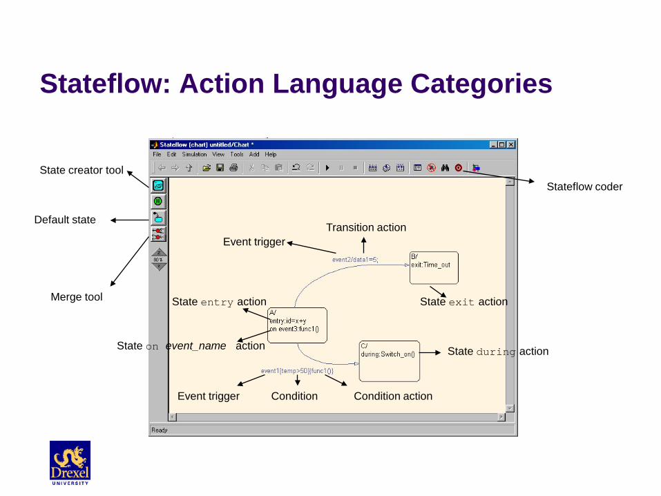
Stateflow: Action Language Categories

Event triggerTransition action

State exit action

State during action

Condition actionConditionEvent trigger

State entry action

State on event_name action

State creator tool

Merge tool

Default state

Stateflow coder

Bouncing Ball

( ) ( )( ) ( ) [ ]

Free fall:

0 Collision:

, 0,1

y g

y t y t

y t cy t c

+ −

+ −

= −

= =

= − ∈

Power Conditioning System

High power drives in vehicle applications Startup (precharge) Normal (current regulation) Shutdown (bleed)

Background (Boost converters) M. Senesky, G. Eirea, and T. J. Koo, "Hybrid Modeling and Control of Power

Electronics," in Hybrid Systems: Computation and Control, vol. 2623, Lecture Notes in Computer Science. New York: Springer-Verlag, 2003, pp. 450-465.

P. Gupta and A. Patra, "Hybrid Sliding Mode Control of DC-DC Power Converters," presented at IEEE Tencon 2003, Bangalore, 2003.

Li

C ov+-E

oR

bleedRpreR

Power Conditioning System

1s

Time

Synch

Step1

Step

Scope

Total Load Current

Main Breaker

Precharge

Bleed

Bank Voltage

Mains Voltage

Mains Current

Bank Current

Power System

Power

1

On

-1

Off

Voltage

I_av ge

Time

MainBreaker

PreBreaker

Bleed

I_av ge_reset

Time_reset

Modes1Memory2

Memory1

Memory

10

Gain

0

Display

1

Constant1

Clock

1s

Avge Current

MainBreaker {OFF=-1, ON=1}MainBreaker {OFF=-1, ON=1}

PreBreaker {OFF=-1, ON=1}PreBreaker {OFF=-1, ON=1}

Bank Voltage

Mains Voltage

Mains Current

Bank Current

Bleed Breaker {OFF=-1, ON=1}Bleed Breaker {OFF=-1, ON=1}Av ge Current Reset

Av ge Current Reset

Time Reset

I_av ge

Time

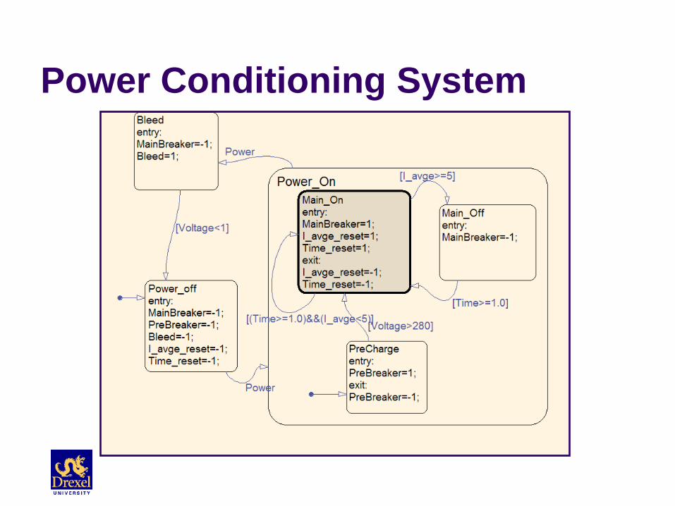
Power Conditioning System

Power Conditioning System

Inverted Pendulum ~ 1

22 cos sincos sin

Suppose we choose to regulate , so that thependulum equations are

sin coswhere is treated as a control.

x v

v Fv

F v

uu

θ ω

θω ω θθ ω θ

θ ωω θ θ

=

=

+ = ++ =

== −

Inverted Pendulum ~ 2

[ ]

Suppose we wish to design a global feedback controller that will steer any initial state to the upright positionwith the constraint 1,1 .

Feedback linearization will not work in general, choose so t

u

u

∈ −

hatsin cos 0 2 0

2 sin within constraints only near 0.cos

u

u

θ θ θ θ θ θ

θ θ θ θθ

− + = → + + =

− − −⇒ = =

Inverted Pendulum Swing-up Strategy

( )

[ ]( )

212, sin cos cos 1

0 when 0, 0

1) pump/remove energy into system until 0, ,

sin cos sin cos2) wait until pendulum is close to upright3) apply feedback

pend

pend

pend pend

u EE

E E

E u u

θ ω ω θ θ ω θ

ω θ

ε ε

ω θ θ θω ω θ

= = − = + −

= = =

≈ ∈ −

= − − = −

linearizing control

Inverted Pendulum: Control Strategy

Constant energy trajectories, 0,in 'wait' state. Switch to 'stabilize' inblue box.

u =

Brockett’s Necessary Condition

Necessary Condition for Asymptotic Stability

( ) ( )

( )( )( ) ( )( )

, , , , 0,0 0: (Brockett) Suppose is smooth and the origin is

stabilized by a smooth state feedback control ,

0 0. Then the mapping : ,

, maps neighborhoods of the origi

n m

n n

x f x u x R u R ff

u x

u F R R

F x f x u x

= ∈ ∈ =

= →

=

Theorem

( )( )

n

into neighborhoods of the origin, i.e.0 0 such that

alternatively, is a neighborhood of 0 .m n

B F B

f B R Rε δ

δ

δ ε∀ > ∃ > ⊂

× ∈

Example 11

2 1

x ux x u==

1.0 0.5 0.5 1.0x1

1.0

0.5

0.5

1.0

x2

1.0 0.5 0.5 1.0F1

1.2

1.0

0.8

0.6

0.4

0.2

0.2F2

Points on F2 axis close to F1 axis are outside image.

Example 2

1 3 1

2 3 1

3 2

2 1

cos cossin sin

Notice that points on the axis close to axisare not in the image of the mapping.

x

x

x v x x udy v x x udt

x u

F F

θθ

θ ω

= = ⇔ = =

Notions of Solution for Discontinuous Dynamics

Solutions of ODEs

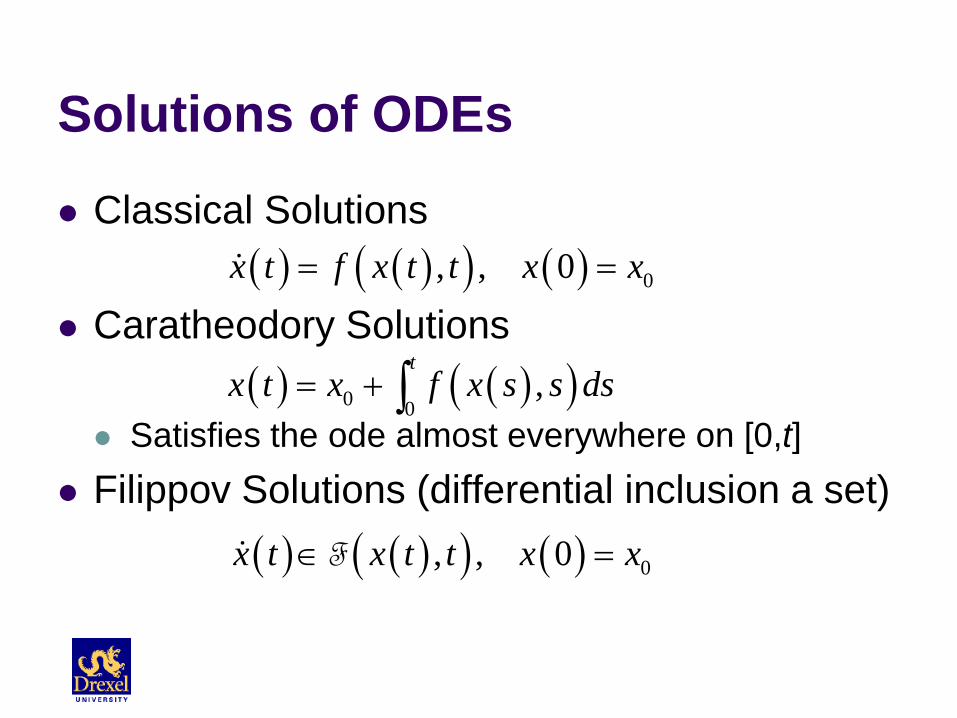
Classical Solutions

Caratheodory Solutions

Satisfies the ode almost everywhere on [0,t] Filippov Solutions (differential inclusion a set)

( ) ( )( ) ( ) 0, , 0x t f x t t x x= =

( ) ( )( )0 0,

tx t x f x s s ds= + ∫

( ) ( )( ) ( ) 0, , 0x t x t t x x∈ =F

Classical Solutions

( ) ( )( )( )

,

: is continuously differenticlassical solution able.

x t f x t t

x t

=

1 2 3 4t

0.2

0.4

0.6

0.8

1.0vtExample: brick on ramp

with stiction.sgn sinmv v cv mgκ θ= − − +

Not a classical solution

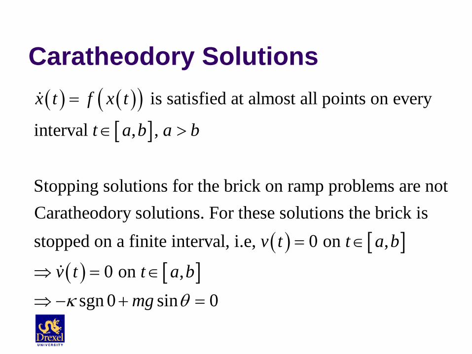
Caratheodory Solutions( ) ( )( )

[ ] is satisfied at almost all points on every

interval , ,

Stopping solutions for the brick on ramp problems are notCaratheodory solutions. For these solutions the brick isstopped on a finite

x t f x t

t a b a b

=

∈ >

( ) [ ]( ) [ ]

interval, i.e, 0 on ,

0 on ,sgn 0 sin 0

v t t a b

v t t a bmgκ θ

= ∈

⇒ = ∈

⇒ − + =

Brick Example – try something else

sgn sin

sgn sin

sin 0

sin , sin 0

sin 0

mv v cv mgcv v v g

m m

cv v g vm m

v g g vm m

cv v g vm m

κ θκ θ

κ θ

κ κθ θ

κ θ

= − − + ⇒

= − − +

= − − + >

∈ − + + =

= − + <

Filippov Solutions

0

( ) ( ( ), ) : conv ( ( , ( )) ( , ( )), )dx t x t t f S x t x t tdt δ

δ δ>

∈ = −ΛF

{ }}:),( δδ <−∈= xyRyxS n

( , ) : subset of measure zero on which is not definedx fδΛ

((

Example: nearest neighbor 3 agents moving in square

Q Rule: move diametrically

away from nearest neighbor

{ } { }{ }1 2 3

Nearest neighbor to

arg min , , \

Action

i

i i i

i ii

i i

p

p q q Q p p p p

pp

p

= − ∈∂ ∪

−=

−

N

N

N

Example: nearest neighbor, cont’d Consider 1 agent - in which case

the only obstacles are the walls. The nearest neighbor is easily

identified on the nearest wall. The vector field is well defined

everywhere except on the diagonals where it is not defined because there are multiple nearest neighbors.

11

1

p qpp q−

=−

Example: nearest neighbor, cont’d

( )

( )( )( )( )

2 1 2

1 2 11 2

2 1 2

1 2 1

0, 11,0

,0,11,0

x x xx x x

x f x xx x xx x x

− − < < − − < <= = < < − < < −

( )0 1

1 , 0 11 0

f α α α

∈ + − ≤ ≤

Extension of Brockett’s Condition

( )( )

( ) ( )( )

( )( )

Assumption on , :

convex , convex

conv , ,conv

: Admissible feedback controls are piecewise continuous andsolutions are defined in the sense of Filippov

,

m n

m

f x u

A R f x A R

A R f x A f x A

u x

x f x u x

⊆ ⇒ ⊆

∀ ⊆ ⊆

∈

Definition

F

( )( )

( )

and 0 0

(Ryan): For , continuous and satisfying assumption, asymptoticstabilization by discontinuous feedback each neighborhood

of 0 , is a neighborhood of 0 .n m n

u

f x u

R f R R

∈

⇒

∈ × ∈

Theorem

F

B

B