Variable Selection for Model-Based Clustering

Adrian E. Raftery, Nema Dean1

Technical Report no. 452

Department of StatisticsUniversity of Washington

May 10, 2004

1Adrian E. Raftery is Professor of Statistics and Sociology, and Nema Dean is Grad-

uate Research Assistant, both at the Department of Statistics, University of Washington,

Box 354322, Seattle, WA 98195-4322. Email: raftery/nemad@stat.washington.edu, Web:

www.stat.washington.edu/raftery. This research was supported by NIH grant 8 R01 EB002137-

02. The authors are grateful to Chris Fraley and Peter Smith for helpful comments.

Abstract

We consider the problem of variable or feature selection for model-based clustering. We recastthe problem of comparing two nested subsets of variables as a model comparison problem,and address it using approximate Bayes factors. We develop a greedy search algorithmfor finding a local optimum in model space. The resulting method selects variables (orfeatures), the number of clusters, and the clustering model simultaneously. We applied themethod to several simulated and real examples, and found that removing irrelevant variablesoften improved performance. Compared to methods based on all the variables, our variableselection method consistently yielded more accurate estimates of the number of clusters, andlower classification error rates, as well as more parsimonious clustering models and easiervisualization of results.

Keywords: Bayes factor, BIC, Feature selection, Model-based clustering, Unsupervisedlearning, Variable selection

Contents

1 Introduction 1

2 Methodology 2

2.1 Model-Based Clustering . . . . . . . . . . . . . . . . . . . . . . . . . . . . . . . . . . 2

2.2 Model-Based Variable Selection . . . . . . . . . . . . . . . . . . . . . . . . . . . . . . 3

2.3 Combined Variable Selection and Clustering Procedure . . . . . . . . . . . . . . . . . 6

3 Simulation Examples 7

3.1 First Simulation Example: Two Clusters . . . . . . . . . . . . . . . . . . . . . . . . . 7

3.2 Second Simulation Example: Irrelevant Variables Correlated with Clustering Variables 9

4 Examples 10

4.1 Leptograpsus Crabs Data . . . . . . . . . . . . . . . . . . . . . . . . . . . . . . . . . 12

4.2 Iris Data . . . . . . . . . . . . . . . . . . . . . . . . . . . . . . . . . . . . . . . . . . . 14

4.3 Texture Dataset . . . . . . . . . . . . . . . . . . . . . . . . . . . . . . . . . . . . . . 15

5 Discussion 17

List of Tables

1 Parameterisations of the Covariance Matrix in the mclust Software . . . . . . . . . . 3

2 Individual Step Results from greedy search algorithm for First Simulation . . . . . . 8

3 Classification Results for the First Simulation Example . . . . . . . . . . . . . . . . . 9

4 Individual Step Results from greedy search algorithm for Second Simulation . . . . . 11

5 Classification results for the Second Simulation Example . . . . . . . . . . . . . . . . 11

6 Classification Results for the Crabs Data . . . . . . . . . . . . . . . . . . . . . . . . . 12

7 Classification Results for the Iris Data . . . . . . . . . . . . . . . . . . . . . . . . . . 15

8 Texture Example: Confusion matrix for the clustering based on the selected variables. 16

9 Classification Results for the Texture Data . . . . . . . . . . . . . . . . . . . . . . . 17

List of Figures

1 Graphical Representation of Models M1 and M2 for Clustering Variable Selection . . 5

2 First Simulation Example: Pairs plot of the data . . . . . . . . . . . . . . . . . . . . 7

3 Second Simulation Example: Pairs plot of 8 of the 15 variables. . . . . . . . . . . . . 10

i

1 Introduction

In classification, or supervised learning problems, the structure of interest may often be

contained in only a subset of the available variables and inclusion of unnecessary variables

in the learning procedure may degrade the results. In these cases some form of variable

selection prior to, or incorporated into the fitting procedure may be advisable. Similarly,

in clustering, or unsupervised learning problems, the structure of greatest interest to the

investigator may be best represented using only a few of the feature variables. However,

in clustering the classification is not observed, and there is usually little or no a priori

knowledge of the structure being looked for in the analysis, so there is no simple pre-analysis

screening technique available to use. In this case it makes sense to consider including the

variable selection procedure as part of the clustering algorithm.

In this paper, we introduce a method for variable or feature selection for model-based

clustering. The basic idea is to recast the variable selection problem as one of comparing

competing models for all the variables initially considered. Comparing two nested subsets

is equivalent to comparing a model in which all the variables in the bigger subset carry

information about cluster membership, with a model in which the variables considered for

exclusion are conditionally independent of cluster membership given the variables included

in both models. This comparison is made using approximate Bayes factors. This model

comparison criterion is combined with a greedy search algorithm to give an overall method

for variable selection. The resulting method selects the clustering variables, the number of

clusters, and the clustering model simultaneously.

The variable selection procedure suggested in this paper is tailored specifically for model-

based clustering and, as such, incorporates the advantages of this paradigm relative to some

of the more heuristic clustering algorithms. They include an automatic method for choosing

the number of clusters, only one user-defined input necessary (the maximum number of

clusters to be considered) that is easily interpretable, and a basis in statistical inference.

A brief review of model-based clustering is given in Section 2.1. The statistical model

behind the variable selection method is explained in Section 2.2 and the greedy search al-

gorithm is introduced in Section 2.3. In Section 3 some simulation results comparing the

performance of model-based clustering with and without variable selection are presented.

In Section 4 model-based clustering with and without variable selection is applied to some

sample real data sets and the results are compared. A discussion of the advantages and

limitations of the overall method is presented in the final section, which also discusses some

other approaches to the problem.

1

2 Methodology

2.1 Model-Based Clustering

Model-based clustering is based on the idea that, instead of coming from a single population,

the observed data come from a source with several subpopulations. The general idea is to

model each of the subpopulations separately and the overall population as a mixture of these

subpopulations, using finite mixture models. Model-based clustering goes back at least to

Wolfe (1963) and reviews of the area are given by McLachlan and Peel (2000) and Fraley

and Raftery (2002).

The general form of a finite mixture model with G subpopulations or groups is

f(x) =G∑

g=1

πgfg(x),

where the πg’s are called the mixing proportions and represent the prior probability of an

observation coming from each group g, and the fg(·)’s are the densities of the groups. The

subpopulations are often modeled by members of the same parametric density family, so the

finite mixture model can be written

f(x) =G∑

g=1

πgf(x|φg),

where the φg’s are the parameter vectors for each group.

In practice, with continuous data, multivariate normal densities are often used to model

the components, that is f(·|φg) = MV N(·|µg, Σg). The covariance matrix can be decom-

posed, as in Banfield and Raftery (1993) and Celeux and Govaert (1995), into the following

form

Σg = λgDgAgDg,

where λg is the largest eigenvalue of Σg and controls the volume of the gth cluster, Dg is the

matrix of eigenvectors of Σg, which control the orientation of that cluster and Ag is a diagonal

matrix with the scaled eigenvalues as entries, which control the shape of that cluster. By

imposing constraints on the various elements of this decomposition, a large range of models

is available ranging from the simple spherical models which have fixed shape, to the least

parsimonious model where all elements of the decomposition are allowed to vary across all

clusters. A list of the models available in the mclust software (Fraley and Raftery 2003) is

given in Table 1.

2

Table 1: Parameterisations of the Covariance Matrix Σg Currently Available in the mclust

Software. When the data are of dimension 1, only two models are available: equal variances(E), and unequal variances (V).

Name Model Distribution Volume Shape OrientationEII λI Spherical equal equal NAVII λgI Spherical variable equal NAEEI λA Diagonal equal equal coordinate axesVEI λgA Diagonal variable equal coordinate axesEVI λAg Diagonal equal variable coordinate axesVVI λgAg Diagonal variable variable coordinate axesEEE λDADT Ellipsoidal equal equal equalVVV λgDgAgD

Tg Ellipsoidal variable variable variable

EEV λDgADTg Ellipsoidal equal equal variable

VEV λgDgADTg Ellipsoidal variable equal variable

One of the difficulties of some of the more heuristic clustering algorithms is the lack

of a statistically principled method for determining the number of clusters. Since it is an

inferentially based procedure, model-based clustering can use model selection methods to

make this decision. Bayes factors, the ratio of posterior to prior odds for the models, are

used to compare models. This means that the models to be compared can be non-nested.

Since Bayes factors are usually difficult to compute, the difference between the Bayesian

information criterion (BIC) for the competing models is used to approximate twice the

logarithm of the Bayes factors. This is defined by

BIC = 2 × log(maximized likelihood) − (no. of parameters) × log(n), (1)

where n is the number of observations. We choose the number of groups and parametric

model by recognizing that each different combination of number of groups and parametric

constraints defines a model, which can then be compared to others. Keribin (1998) showed

this to be consistent for the choice of the number of clusters. Differences of less than 2

between BIC values are typically viewed as barely worth mentioning, while differences greater

than 10 are often regarded as constituting strong evidence (Kass and Raftery 1995).

2.2 Model-Based Variable Selection

To address the variable selection problem, we recast it as a model selection problem. We

have a data set Y , and at any stage in our variable selection algorithm, it is partitioned into

3

three sets of variables, Y (1), Y (2) and Y (3), namely:

• Y (1): the set of already selected clustering variables,

• Y (2): the variable(s) being considered for inclusion into or exclusion from the set of

clustering variables, and

• Y (3): the remaining variables.

The decision for inclusion or exclusion of Y (2) from the set of clustering variables is then

recast as one of comparing the following two models for the full data set:

M1 : p(Y |z) = p(Y (1), Y (2), Y (3)|z)

= p(Y (3)|Y (2), Y (1))p(Y (2)|Y (1))p(Y (1)|z) (2)

M2 : p(Y |z) = p(Y (1), Y (2), Y (3)|z)

= p(Y (3)|Y (2), Y (1))p(Y (2), Y (1)|z),

where z is the (unobserved) set of cluster memberships. Model M1 specifies that, given Y (1),

Y (2) is conditionally independent of the cluster memberships (defined by the unobserved

variables z), that is, Y (2) gives no additional information about the clustering. Model M2

implies that Y (2) does provide additional information about clustering membership, after

Y (1) has been observed. If Y (2) consists of only one variable, then p(Y (2)|Y (1)) in model M1

represents a linear regression model. The difference between the assumptions underlying the

two models is illustrated in Figure 1, where arrows indicate dependency.

Models M1 and M2 are compared via an approximation to the Bayes factor which allows

the high-dimensional p(Y (3)|Y (2), Y (1)) to cancel from the ratio, leaving only the clustering

and regression integrated likelihoods. The integrated likelihood, as given below in (3), is

often difficult to calculate exactly, so we use the BIC approximation (1).

The Bayes factor, B12, for M1 against M2 based on the data Y is defined as

B12 = p(Y |M1)/p(Y |M2),

where p(Y |Mk) is the integrated likelihood of model Mk (k = 1, 2), namely

p(Y |Mk) =∫

p(Y |θk, Mk)p(θk|Mk)dθk. (3)

In (3), θk is the vector-valued parameter of model Mk, and p(θk|Mk) is its prior distribution

(Kass and Raftery 1995).

4

M2M1

Z Z

Y1 Y2 Y1 Y2

Y3Y3

Figure 1: Graphical Representation of Models M1 and M2 for Clustering Variable Selection.In model M1, the candidate set of additional clustering variables, Y (2), is conditionallyindependent of the cluster memberships, z, given the variables Y (1) already in the model. Inmodel M2, this is not the case. In both models, the set of other variables considered, Y (3), isconditionally independent of cluster membership given Y (1) and Y (2), but may be associatedwith Y (1) and Y (2).

Let us now consider the integrated likelihood of model M1, p(Y |M1) = p(Y (1), Y (2), Y (3)|M1).

From (2), the model M1 is specified by three probability distributions: the finite mixture

model that specifies p(Y (1)|θ1, M1), and the conditional distributions p(Y (2)|Y (1), θ1, M1) and

p(Y (3)|Y (2), Y (1), θ1, M1), the latter two being multivariate regression models. We denote the

parameter vectors that specify these three probability distributions by θ11, θ12, and θ13, and

we take their prior distributions to be independent. It follows that the integrated likelihood

itself factors:

p(Y |M1) = p(Y (3)|Y (2), Y (1), M1) p(Y (2)|Y (1), M1) p(Y (1)|M1), (4)

where p(Y (3)|Y (2), Y (1), M1) =∫

p(Y (3)|Y (2), Y (1), θ13, M1) p(θ13|M1)dθ13, and similarly for

p(Y (2)|Y (1), M1) and p(Y (1)|M1). Similarly, we obtain

p(Y |M2) = p(Y (3)|Y (2), Y (1), M2) p(Y (2), Y (1)|M2), (5)

where p(Y (2), Y (1)|M2) is the integrated likelihood for the model-based clustering model for

(Y (2), Y (1)) jointly.

The conditional distribution of (Y (3)|Y (2), Y (1)) is unaffected by the distribution of (Y (2), Y (1)),

and so the prior distribution of its parameter, θ13, should be the same under M1 as under

M2. It follows that p(Y (3)|Y (2), Y (1), M2) = p(Y (3)|Y (2), Y (1), M1). We thus have

B12 =p(Y (2)|Y (1), M1)p(Y (1)|M1)

p(Y (2), Y (1)|M2), (6)

5

which has been greatly simplified by the cancellation of the factors involving the potentially

high-dimensional Y (3).

The integrated likelihoods in (6) are hard to evaluate analytically, and so we use the

BIC approximation of (1) to approximate them. For the model-based clustering integrated

likelihoods, p(Y (1)|M1) and p(Y (2), Y (1)|M2), these take the form (1); see, for example, Fraley

and Raftery (2002).

In our implementation, we consider only the case where Y (2) contains just one variable,

in which case p(Y (2)|Y (1), M1) represents a linear regression model. The BIC approximation

to this term in (6) is

2 log p(Y (2)|Y (1), M1) ≈ BICreg = −n log(2π) − n log(RSS/n) − n − (dim(Y (1)) + 2) log(n),

(7)

where RSS is the residual sum of squares in the regression of Y (2) on the variables in Y (1).

This is an important aspect of the model formulation, since it does not require that irrelevant

variables be independent of the clustering variables. If instead the independence assumption

p(Y (2)|Y (1)) = p(Y (2)) were used, we would be quite likely to include variables that were

related to the clustering variables, but not necessarily to the clustering itself.

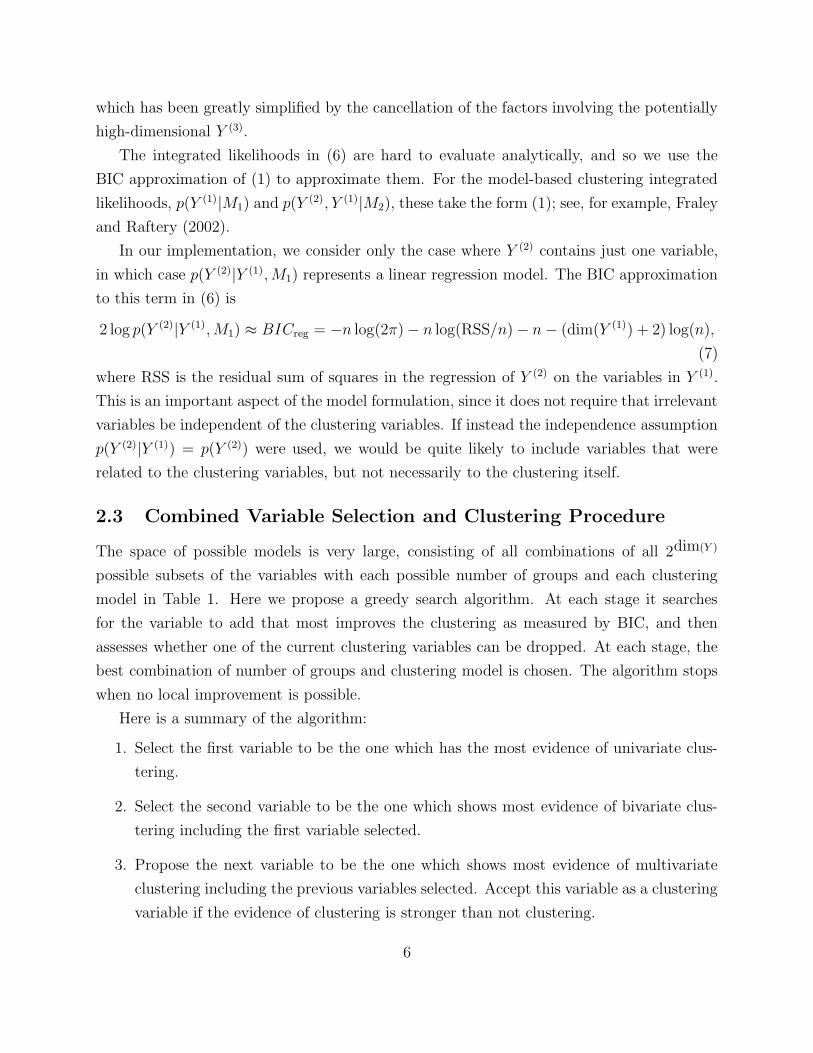
2.3 Combined Variable Selection and Clustering Procedure

The space of possible models is very large, consisting of all combinations of all 2dim(Y )

possible subsets of the variables with each possible number of groups and each clustering

model in Table 1. Here we propose a greedy search algorithm. At each stage it searches

for the variable to add that most improves the clustering as measured by BIC, and then

assesses whether one of the current clustering variables can be dropped. At each stage, the

best combination of number of groups and clustering model is chosen. The algorithm stops

when no local improvement is possible.

Here is a summary of the algorithm:

1. Select the first variable to be the one which has the most evidence of univariate clus-

tering.

2. Select the second variable to be the one which shows most evidence of bivariate clus-

tering including the first variable selected.

3. Propose the next variable to be the one which shows most evidence of multivariate

clustering including the previous variables selected. Accept this variable as a clustering

variable if the evidence of clustering is stronger than not clustering.

6

4. Propose the variable for removal from the current set of selected variables to be the one

which shows least evidence of multivariate clustering including all variables selected

versus only multivariate clustering on the other variables selected and not clustering

on the proposed variable. Remove this variable from the set of clustering variables if

the evidence of clustering is weaker than not clustering.

5. Iterate steps 3 and 4 until two consecutive steps have been rejected, then stop.

3 Simulation Examples

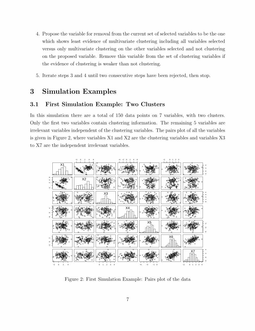
3.1 First Simulation Example: Two Clusters

In this simulation there are a total of 150 data points on 7 variables, with two clusters.

Only the first two variables contain clustering information. The remaining 5 variables are

irrelevant variables independent of the clustering variables. The pairs plot of all the variables

is given in Figure 2, where variables X1 and X2 are the clustering variables and variables X3

to X7 are the independent irrelevant variables.

X1

−2 0 2 4 6 −4 −2 0 2 4 6 −2 0 1 2 3

−2

02

4

−2

24

6

X2

X3

01

23

4

−4

04 X4

X5

−5

−3

−1

−2

02 X6

−2 0 2 4 0 1 2 3 4 −5 −3 −1 0 −2 0 1 2 3 4

−2

02

4

X7

Figure 2: First Simulation Example: Pairs plot of the data

7

For the clustering on all 7 variables BIC chooses a five-group diagonal EEI model. The

next model is a 4-group EEI model. The closest two-group model in terms of BIC is the

two-group EEE model but there is a substantial difference of 20 points between this and the

model with highest BIC. This would lead to the (incorrect) choice of a five group structure

for this data. The step by step progress of the greedy search selection procedure is shown

in Table 2. Two variables are chosen, X1 and X2; these are the correct clustering variables.

The model with the decisively highest BIC for clustering on these variables is the two-group

VVV model, which gives both the correct number of groups and the correct clustering model.

Table 2: Individual Step Results from greedy search algorithm for First Simulation. TheBIC difference is the difference between the BIC for clustering and the BIC for not clusteringfor the best variable proposed, as given in (8).

Step Best variable Proposed BIC Model Number of Resultno. proposed for difference chosen clusters chosen1 X2 inclusion 15 V 2 Included2 X1 inclusion 136 VVV 2 Included3 X6 inclusion -13 VVV 2 Not included4 X1 exclusion 136 VVV 2 Not excluded

Since the data are simulated, we know the underlying group memberships of the observa-

tions, and we can check the quality of the clustering in this way. Clustering on the selected

two variables gives 100% correct classification. The confusion matrix for the clustering on

all variables is as follows:Group1 Group2

Cluster1 53 0Cluster2 4 30Cluster3 34 0Cluster4 1 13Cluster5 0 15

The error rate is 44.7%. This is calculated by taking the best matches of clusters with the

groups (i.e. Group 1 ↔ Cluster 1 and Group 2 ↔ Cluster 2), which gives us the minimum

error rate over all matches between clusters and groups. If we were to correctly amalgamate

clusters 1 and 3 and identify them as one group, and to amalgamate clusters 2, 4 and 5 and

identify them as another group, we would get an error rate of 3.3%. However, this assumes

knowledge that the investigator would not typically have in practice.

Finally we pretend we know the number of groups (2) correctly in advance (as do many

8

heuristic clustering algorithms) and cluster on all the variables allowing only two-group

models. The two-group model with the highest BIC is the EEE model, and this has an error

rate of 3.3%.

In this example, variable selection led to a clustering method that gave the correct number

of groups and a 0% error rate. Using all variables led to a considerable overestimation of the

number of groups, and a large error rate. Even when the five groups found in this way were

optimally combined into two groups, or when the correct number of groups was assumed

known, clustering using all the variables led to a nonzero error rate, with 5 errors.

Table 3: Classification Results for the First Simulation Example. The correct number ofgroups was 2. (c) denotes constrained to this number of groups

Variable Selection Number Number ErrorProcedure of variables of Groups rate (%)

None-All variables 7 5 44.7None-All variables 7 2(c) 3.3

Greedy search 2 2 0

3.2 Second Simulation Example: Irrelevant Variables Correlatedwith Clustering Variables

Again we have a total of 150 points from two clustering variables, with two groups. To

make the problem more difficult we allow different types of irrelevant variables. There are

three independent irrelevant variables, seven irrelevant variables which are allowed to be

dependent on other irrelevant variables, and three irrelevant variables which have a linear

relationship with either or both of the clustering variables. This gives a total of thirteen

irrelevant variables.

The pairs plot of a selection of the variables is given in Figure 3. Variables X1 and X2 are

the clustering variables, X3 is an independent irrelevant variable, X6 and X7 are irrelevant

variables that are correlated with one another, X13 is linearly dependent on the clustering

variable X1, X14 is linearly dependent on the clustering variable X2, and X15 is linearly

dependent on both clustering variables, X1 and X2.

For the clustering on all 15 variables BIC chooses a two-group diagonal EEI model. The

next model is a three-group diagonal EEI model, with a difference of 10 points between the

two. In this case the investigator would probably decide on the correct number of groups,

9

X1

−2 0 2 4 6 −3 −1 0 1 2 −4 −2 0 2 −6 −2 2 4

−4

04

−2

26 X2

X3

−2

02

4

−3

−1

1 X6

X7

−3

02

−4

02 X13

X14

04

8

−4 −2 0 2 4

−6

−2

2

−2 0 1 2 3 4 −3 −1 1 3 0 2 4 6 8

X15

Figure 3: Second Simulation Example: Pairs plot of 8 of the 15 variables.

based on this evidence. The error rate for classification based on this model is 1.3%.

The results of the steps when the greedy search selection procedure is run are given in

Table 4. Two variables are selected, and these are precisely the correct clustering variables.

The model with the highest BIC for clustering on these variables is a two-group VVV model

with the next highest model being the three-group VVV model. There is a difference of 27

between the two BIC values, which would typically be regarded as strong evidence.

We compare the clustering memberships with the underlying group memberships and find

that clustering on the selected variables gives a 100% correct classification, i.e. no errors. In

contrast, using all 15 variables gives a nonzero error rate, with two errors. Variable selection

has the added advantage in this example that it makes the results easy to visualize, as only

two variables are involved after variable selection.

4 Examples

We now give the results of applying our variable selection method to three real datasets

where the correct number of clusters is known.

10

Table 4: Individual Step Results from greedy search algorithm for Second Simulation. TheBIC difference is the difference between the BIC for clustering and the BIC for not clusteringfor the best variable proposed, as given in (8).

Step Best variable Proposed BIC Model Number of Resultno. proposed for difference chosen clusters chosen1 X11 inclusion 17 V 2 Included2 X2 inclusion 5 EEE 2 Included3 X1 inclusion 109 VVV 2 Included4 X11 exclusion -19 VVV 2 Excluded5 X4 inclusion -9 VVV 2 Not included6 X2 exclusion 153 VVV 2 Not excluded

Table 5: Classification results for the Second Simulation Example

Variable Selection Number Number ErrorProcedure of variables of Groups rate (%)

None-All variables 15 2 1.3Greedy search 2 2 0

11

4.1 Leptograpsus Crabs Data

This dataset consists of 200 subjects: 100 of species orange (50 male and 50 female) and

100 of species blue (50 male and 50 female), so we are hoping to find a four-group cluster

structure. There are five measurements on each subject: width of frontal lip (FL), rear width

(RW), length along the mid-line of the carapace (CL), maximum width of the carapace (CW)

and body depth (BD) in mm. The dataset was published by Campbell and Mahon (1974),

and was further analyzed by Ripley (1996) and McLachlan and Peel (1998, 2000).

The variables selected by the variable selection procedure were (in order of selection)

CW, RW, FL and BD. The error rates for the different clusterings are given in Table 6.

The error rates for the nine-group and six-group models were the minimum error rates over

all matchings between clusters and groups, where each group was matched with a unique

cluster.

Table 6: Classification Results for the Crabs Data. The correct number of groups is 4. (c)indicates that the number of groups was constrained to this value in advance. The error ratesfor the 9 and 6-group models were calculated by optimally matching clusters to groups.

Original VariablesVariable Selection Number Number Model Error

Procedure of variables of Groups selected rate (%)None-All variables 5 9 EEE 45.5None-All variables 5 4(c) EEE 39.5

Greedy search 4 4 EEV 7.5Principal Components

Variable Selection Number Number Model ErrorProcedure of components of Groups selected rate (%)

None-All components 5 6 EEI 34.5None-All components 5 4(c) EEE 39.5

Greedy search 3 4 EEV 6.5

When no variable selection was done, the number of groups was substantially overesti-

mated, and the error rate was 45.5%, as can be seen in the confusion matrix for clustering

12

on all variables:Group1 Group2 Group3 Group4

Cluster1 34 0 0 0Cluster2 0 28 0 0Cluster3 0 0 22 5Cluster4 0 0 0 25Cluster5 7 6 0 0Cluster6 0 0 0 20Cluster7 9 16 0 0Cluster8 0 0 12 0Cluster9 0 0 16 0

When no variable selection was done, but the number of groups was assumed to be correctly

known in advance, the error rate was still very high (39.5%), as can be seen in the confusion

matrix for the clustering on all variables, with the number of groups restricted to be 4:

Group1 Group2 Group3 Group4Cluster1 31 0 25 0Cluster2 0 34 0 14Cluster3 19 15 25 5Cluster4 0 1 0 31

When our variable selection method was used, the correct number of groups was selected,

and the error rate was much lower (7.5%), as can be seen in the confusion matrix for the

clustering on the selected variables:

Group1 Group2 Group3 Group4Cluster1 40 0 0 0Cluster2 10 50 0 0Cluster3 0 0 50 5Cluster4 0 0 0 45

This is a striking result, especially given that the method selected four of the five variables,

so not much variable selection was actually done in this case.

In clustering, it is common practice to work with principal components of the data, and

to select the first several, as a way of reducing the data dimension. Our method could be

used as a way of choosing the principal components to be used, and it has the advantage

that one does not have to use the principal components that explain the most variation, but

can automatically select the principal components that are most useful for clustering. To

illustrate this, we computed the five principal components of the data and used these instead

of the variables. The variable selection procedure chose (in order) principal components 3,

2 and 1.

13

Once again, when all the principal components were used, the number of groups was

overestimated, and the error rate was high, at 34.5%. When the number of groups was

assumed to be correctly known in advance but no variable selection was done, the error rate

was even higher, at 39.5%. When variable selection was carried out, our method selected

the correct number of groups without invoking any prior knowledge of it, and the error rate

was much reduced, at 6.5%.

It has been shown that the practice of reducing the data to the principal components that

account for the most variability before clustering is not justified in general. Chang (1983)

showed that the principal components with the larger eigenvalues do not necessarily contain

the most information about the cluster structure, and that taking a subset of principal

components can lead to a major loss of information about the groups in the data. Chang

demonstrated this theoretically, by simulations, and in applications to real data. Similar

results have been found by other researchers, including Green and Krieger (1995) for market

segmentation, and Yeung and Ruzzo (2001) for clustering gene expression data. Our method

to some extent rescues the principal component dimension reduction approach, as it allows

one to use all or many of the principal components, and then for clustering select only those

that are most useful for clustering, not those that account for the most variance. This avoids

Chang’s criticism.

4.2 Iris Data

The well-known iris data consist of 4 measurements on 150 samples of either Iris Setosa,

Iris Versicolor or Iris Virginica (Anderson 1935; Fisher 1936). The measurements are sepal

length, sepal width, petal length and petal width (cm). When one clusters using all the

variables, the model with the highest BIC is the two-group VEV model, with the three-

group VEV model within one BIC point of it. The confusion matrix from the two-group

clustering is as follows:

Setosa V ersicolor V irginicaCluster1 50 0 0Cluster2 0 50 50

It is clear that the setosa group is well picked out but that versicolor and virginica have been

amalgamated. This will lead to a minimum error of 33.3%.

14

The confusion matrix from the three-group clustering is as follows:

Setosa V ersicolor V irginicaCluster1 50 0 0Cluster2 0 45 0Cluster3 0 5 50

This gives a 3.3% error rate and reasonable separation. However, given the BIC values, an

investigator with no reason to do otherwise would have erroneously chosen the two-group

model with poor results.

The variable selection procedure selects three variables (all but sepal length) which gives

the highest BIC model to be three-group VEV model with the next highest model being the

four-group VEV model with a difference of 14. The confusion matrix from the three-group

clustering on these variables is as follows:

Setosa V ersicolor V irginicaCluster1 50 0 0Cluster2 0 44 0Cluster3 0 6 50

which is a 4% error rate. A summary of the results of the different methods is given in Table

7.

Table 7: Classification Results for the Iris Data. The correct number of groups is oftenconsidered to be 3. (c) indicates that the number of groups was constrained to this value inadvance.

Variable Selection Number Number ErrorProcedure of variables of Groups rate (%)

None-All variables 4 2 33.3None-All variables 4 3(c) 3.3

Greedy search 3 3 4

4.3 Texture Dataset

The Texture dataset was produced by the Laboratory of Image Processing and Pattern

Recognition (INPG-LTIRF) in the development of the Esprit project ELENA No. 6891

and the Esprit working group ATHOS No. 6620. The original source was Brodatz (1966).

This dataset consists of 5500 observations with 40 variables, created by characterizing each

15

pattern using estimation of fourth order modified moments, in four orientations: 0, 45, 90

and 135 degrees; see Guerin-Dugue and Avilez-Cruz (1993) for details. There are eleven

classes of types of texture: grass lawn, pressed calf leather, handmade paper, raffia looped

to a high pile, cotton canvas, pigskin, beach sand, another type of beach sand, oriental straw

cloth, another type of oriental straw cloth, and oriental grass fiber cloth (labelled groups 1

to 11 respectively). We have 500 observations in each class.

When we cluster on all available variables we find that the model with highest BIC is the

one-cluster model (with an error rate of 90.9%). When we use the greedy search procedure

with a maximum number of 15 clusters (and only allow the unconstrained VVV model since

the search space is already so large), we select 32 variables which, when clustered allowing

all models, decisively choose (via BIC) the 14-cluster VVV model.

The classification matrix for the model on the selected variables is given in Table 8 below.

Table 8: Texture Example: Confusion matrix for the Clustering Based on the SelectedVariables. The largest count in each row is boxed.

Gp 2 Gp 5 Gp 4 Gp 7 Gp 3 Gp 11 Gp 10 Gp 8 Gp 9 Gp 1 Gp 6

Cl 4 500 0 0 0 0 0 0 0 0 0 0

Cl 10 0 500 0 0 0 0 0 0 0 0 0

Cl 11 0 0 496 0 0 0 0 0 0 0 0

Cl 3 0 0 0 491 0 0 0 0 0 10 0

Cl 8 0 0 0 0 484 0 0 0 0 0 0

Cl 6 0 0 0 0 0 467 0 0 0 0 0

Cl 14 0 0 0 0 0 0 435 0 0 0 0

Cl 9 0 0 4 4 0 33 65 38 0 0 9

Cl 7 0 0 0 0 0 0 0 336 0 0 248

Cl 12 0 0 0 0 0 0 0 0 330 0 0

Cl 13 0 0 0 0 0 0 0 0 170 0 0

Cl 1 0 0 0 0 16 0 0 0 0 180 0

Cl 2 0 0 0 0 0 0 0 0 0 309 0

Cl 5 0 0 0 5 0 0 0 126 0 1 243

This model is much closer in terms of number of groups and classifications to the true

underlying structure. Our error rate is reduced from 90.9% to 16.5% (by optimally associ-

ating each group with one of the 14 clusters). We can see that most groups except Group 6

and Group 8 are picked out well. Groups 1 and 9 are picked out as groups with two normal

16

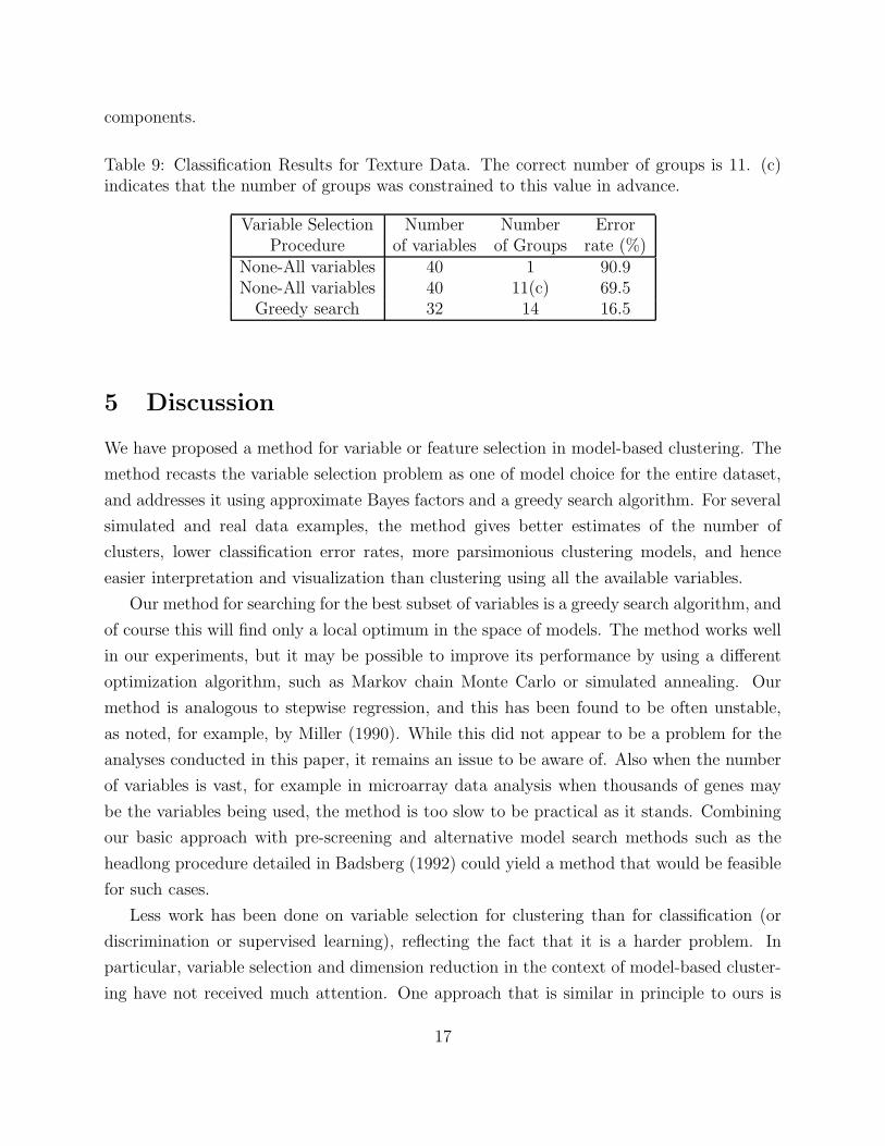
components.

Table 9: Classification Results for Texture Data. The correct number of groups is 11. (c)indicates that the number of groups was constrained to this value in advance.

Variable Selection Number Number ErrorProcedure of variables of Groups rate (%)

None-All variables 40 1 90.9None-All variables 40 11(c) 69.5

Greedy search 32 14 16.5

5 Discussion

We have proposed a method for variable or feature selection in model-based clustering. The

method recasts the variable selection problem as one of model choice for the entire dataset,

and addresses it using approximate Bayes factors and a greedy search algorithm. For several

simulated and real data examples, the method gives better estimates of the number of

clusters, lower classification error rates, more parsimonious clustering models, and hence

easier interpretation and visualization than clustering using all the available variables.

Our method for searching for the best subset of variables is a greedy search algorithm, and

of course this will find only a local optimum in the space of models. The method works well

in our experiments, but it may be possible to improve its performance by using a different

optimization algorithm, such as Markov chain Monte Carlo or simulated annealing. Our

method is analogous to stepwise regression, and this has been found to be often unstable,

as noted, for example, by Miller (1990). While this did not appear to be a problem for the

analyses conducted in this paper, it remains an issue to be aware of. Also when the number

of variables is vast, for example in microarray data analysis when thousands of genes may

be the variables being used, the method is too slow to be practical as it stands. Combining

our basic approach with pre-screening and alternative model search methods such as the

headlong procedure detailed in Badsberg (1992) could yield a method that would be feasible

for such cases.

Less work has been done on variable selection for clustering than for classification (or

discrimination or supervised learning), reflecting the fact that it is a harder problem. In

particular, variable selection and dimension reduction in the context of model-based cluster-

ing have not received much attention. One approach that is similar in principle to ours is

17

that given by Dy and Brodley (2000) where the feature subset selection is wrapped around

EM clustering with order identification. However, they do not consider an eigenvalue de-

composition formulation, or both forward and backward steps in their search pattern and

there is no explicit model for comparing different feature sets. In a model-based clustering

setting Law, Jain, and Figueiredo (2002) looked at a wrapper method of feature selection

incorporated into the mixture-model formulation. In the first approach each variable is al-

lowed to be independent of the others given the cluster membership (diagonal model in the

Gaussian setting) and irrelevant variables are assumed to have the same distribution regard-

less of cluster membership. The missing data structure of the EM algorithm is used both to

estimate the cluster parameters and to select variables.

Vaithyanathan and Dom (1999) put forward an approach which determines both the

relevant variables and the number of clusters by using an objective function that incorpo-

rates both. The functions used in their paper were integrated likelihood and cross-validated

likelihood. The example given was a multinomial model and no extension for continuous or

ordinal data was suggested.

Liu, Zhang, Palumbo, and Lawrence (2003) proposed a Bayesian approach using MCMC,

in which a principal components analysis or correspondence analysis is carried out first and

a number of components to be examined are selected. Then the components important for

clustering are selected from this subset and clustering is performed simultaneously. The pro-

cedure can also automatically select an appropriate Box-Cox transformation to improve the

normality of the groups. This approach requires that principal components be used where,

in certain cases, investigators may be as interested in the variables important for clustering

as in the clustering itself and this information is not easily available in this approach. Also

the approach assumes the number of clusters/groups to be known.

An entirely different approach is taken by Lazzeroni and Owen (2002), where a two-sided

(both variables and samples) cluster analysis is performed which has variable selection as

an implicit part of the procedure. Variables are allowed to belong to more than one cluster

or to no cluster, and similarly with samples. This was motivated by the analysis of gene

expression data. Along a similar line, Getz, Levine, and Domany (2000) proposed a method

that clusters both variables and samples so that clustering on the subsets found in one will

produce stable, sensible clusters in the other. The procedure is iterative but no details on

the stopping criterion were given.

McLachlan, Bean, and Peel (2002) proposed a dimension reduction method where a

mixture of factor analyzers is used to reduce the extremely high dimensionality of a gene

18

expression problem. Pre-specification of the number of factor analyzers to be used is required.

Other examples of dimension reduction include work by Ding, He, Zha, and Simon (2002)

where cluster membership is used as a “bridge” between reduced dimensional clusters and the

full dimensional clusters and reduces dimensions to one less than the number of clusters. It is

an iterative process, swapping between reduced dimensions and the original space. This work

focuses mainly on the simplest model, spherical Gaussian clustering. Another dimension

reduction technique is given by Chakrabarti and Mehrotra (2000), which uses local rather

than global correlations. There are a number of parameters, such as the maximum dimension

allowed in a cluster, that must be specified, for which the optimal values are not all obvious

from the data.

A different approach taken in Mitra, Murthy, and Pal (2002), is more similar to a filter

selection technique than the wrapper techniques more usually looked at. Since it is a one-

step pre-clustering process with no search involved it is very fast, but it takes no account

of any clustering structure when selecting the variables. In a similar vein Talavera (2000)

uses a filter method of subset selection but has no explicit method of deciding how many

variables should be used.

Several approaches to variable selection for heuristic clustering methods have been pro-

posed. One of the methods of feature selection for the more heuristic distance-based clus-

tering algorithms is given by McCallum, Nigam, and Ungar (2000) which involves switching

between “cheap” and “expensive” metrics. A method for k-means clustering variable se-

lection is given by Brusco and Cradit (2001) which is based on the adjusted RAND index

in order to measure similarity of clusterings produced by different variables. However this

requires prior specification of number of clusters and there are problems when the variables

are highly correlated and there are outliers present in the data. Other methods for variable

selection for heuristic clustering include that of Devaney and Ram (1997), who consider a

stepwise selection search run with the COBWEB hierarchical clustering algorithm.

Friedman and Meulman (2004) approach the problem in terms of maximizing an appro-

priate function in terms of weights of variables and different clusterings. Different weights

are selected depending on the scale of the data for that variable. Since the variables are

weighted, rather than selected or removed, there is no actual dimension reduction although

it does allow emphasis on different variables for different clusters. The number of groups

must be specified by user. Work in a similar vein was done by Gnanadesikan, Kettenring,

and Tsao (1995). A similar idea in terms of weighting variables but with a different function

to be optimized is suggested by Desarbo, Carroll, Clarck, and Green (1984), where the sum

19

of weighted squared distances between data points in groups of variables and a distance

based on linear regression on cluster membership is used as the function.

We have developed and described our method in the context of clustering based on

continuous measurements that can be represented, at least approximately, using normal

distributions. However, the same basic ideas can be applied to variable selection in other

clustering contexts, such as clustering multivariate discrete data using latent class models

(Clogg and Goodman 1984; Becker and Yang 1998), or more generally, Bayesian graphical

models with a hidden categorical node (Chickering and Heckerman 1997). When the present

approach is adapted to these other clustering problems, it should retain the aspects that

make it flexible, especially its ability to simultaneously estimate the number of clusters and

group structure, as well as selecting the clustering variables.

Appendix: Variable Selection and Clustering Algorithm

Here we give a more complete description of the variable selection and clustering algorithm.

• Choose Gmax, the maximum number of clusters to be considered for the data.

• First step : The first clustering variable is chosen to be the one which gives the

greatest difference between the BIC of clustering on it (maximized over number of

groups from 2 up to Gmax and different parameterisations) and BIC of no clustering

(single group structure maximized over different parameterisations) on it, where each

variable is looked at separately. We do not require that the greatest difference be

positive.

Specifically, we split Y (3) = Y into its variables y1, . . . , yD1. For all j in 1, . . . , D1 we

compute the approximation to the Bayes factor in (6) by

BICdiff(yj) = BICclust(y

j) − BICnot clust(yj)

where BICclust(yj) = max2≤G≤Gmax,m∈{E,V }{BICG,m(yj)}, with BICG,m(yj) being the

BIC given in (1) for the model-based clustering model for yj with G groups and model

m being either the one-dimensional equal-variance (E) or unequal variance model (V),

and BICnot clust(yj) = BICreg as given in (7) (for a regression model with constant

mean) with dim(Y (1))=0.

We choose the best variable, yj1, such that

j1 = arg maxj:yj∈Y

(BICdiff(yj))

20

and create

Y (1) = (yj1)

and Y (3) = Y \yj1

where Y \yj1 denotes the set of variables in Y excluding variable yj1.

• Second step : Next the set of clustering variables is chosen to be the pair of vari-

ables, including the variable selected in the first step, that gives the greatest difference

between the BIC for clustering on both variables (maximized over number of groups

from 2 up to Gmax and different parameterisations) and the sum of the BIC for the

univariate clustering of the variable chosen in the first step and the BIC for the linear

regression of the new variable on the variable chosen in the first step. Note that we do

not assume that the greatest difference is positive since the only criterion the variables

need to satisfy is being the best initialisation variables.

Specifically, we split Y (3) into its variables y1, . . . , yD2. For all j in 1, . . . , D2 we compute

the approximation to the Bayes factor in (6) by

BICdiff(yj) = BICclust(y

j) − BICnot clust(yj)

where BICclust(yj) = max2≤G≤Gmax,m∈M{BICG,m(Y (1), yj)} with BICG,m(Y (1), yj) be-

ing the BIC given in (1) for the model-based clustering model for the dataset including

both the previously selected variable (contained in Y (1)) and the new variable yj with

G groups and model m in the set of all possible models M , and BICnot clust(yj) =

BICreg + BICclust(Y(1)) where BICreg is given in (7) (the regression model with inde-

pendent variable Y (1) and dependent variable yj) when dim(Y (1))=1 (the number of

variables currently selected) and BICclust(Y(1)) is the BIC for the clustering with only

the currently selected variable in Y (1).

We choose the best variable, yj2, with

j2 = arg maxj:yj∈Y (3)

(BICdiff(yj))

and create

Y (1) = Y (1) ∪ yj2

and Y (3) = Y (3)\yj2

where Y (1) ∪ yj2 denotes the set of variables including those in Y (3) and variable yj2.

21

• General Step [Inclusion part] : The proposed new clustering variable is chosen to

be the variable which gives the greatest difference between the BIC for clustering with

this variable included in the set of currently selected clustering variables (maximized

over numbers of groups from 2 up to Gmax and different parameterisations) and the

sum of the BIC for the clustering with only the currently selected clustering variables

and the BIC for the linear regression of the new variable on the currently selected

clustering variables.

• If this difference is positive the proposed variable is added to the set of selected clus-

tering variables. If not the set remains the same.

Specifically, at step t we split Y (3) into its variables y1, . . . , yDt. For all j in 1, . . . , Dt

we compute the approximation to the Bayes factor in (6) by

BICdiff(yj) = BICclust(y

j) − BICnot clust(yj) (8)

where BICclust(yj) = max2≤G≤Gmax,m∈M{BICG,m(Y (1), yj)}, with BICG,m(Y (1), yj) be-

ing the BIC given in (1) for the model-based clustering model for the dataset including

both the previously selected variables (contained in Y (1)) and the new variable yj with

G groups and model m in the set of all possible models M , and BICnot clust(yj) =

BICreg + BICclust(Y(1)) where BICreg is given in (7) (the regression model with inde-

pendent variables Y (1) and dependent variable yj) when dim(Y (1))= (the number of

variables currently selected) and BICclust(Y(1)) is the BIC for the clustering with only

the currently selected variables in Y (1).

We choose the best variable, yjt, with

jt = arg maxj:yj∈Y (3)

(BICdiff(yj))

and create

Y (1) = Y (1) ∪ yjt if BICdiff(yjt) > 0

and Y (3) = Y (3)\yjt if BICdiff(yjt) > 0

otherwise Y (1) = Y (1) and Y (3) = Y (3).

• General Step [Removal part] : The proposed variable for removal from the set of

currently selected clustering variables is chosen to be the variable from this set which

gives the smallest difference between the BIC for clustering with all currently selected

22

clustering variables (maximized over number of groups greater than 2 up to Gmax and

different parameterisations) and the sum of the BIC for clustering with all currently

selected clustering variables except for the proposed variable and the BIC for the linear

regression of the proposed variable on the other clustering variables.

• If this difference is negative the proposed variable is removed from the set of selected

clustering variables. If not the set remains the same.

In terms of equations for step t + 1, we split Y (1) into its variables y1, . . . , yDt+1. For

all j in 1, . . . , Dt+1 we compute the approximation to the Bayes factor in (6) by

BICdiff(yj) = BICclust − BICnot clust(y

j)

where BICclust = max2≤G≤Gmax,m∈M{BICG,m(Y (1))} with BICG,m(Y (1)) being the BIC

given in (1) for the model-based clustering model for the dataset including the previ-

ously selected variables (contained in Y (1)) with G groups and model m in the set of all

possible models M , and BICnot clust(yj) = BICreg + BICclust(Y

(1)\yj) where BICreg is

given in (7) (the regression model with independent variables being all of Y (1) except

yj and dependent variable yj) when dim(Y (1))= (the number of variables currently

selected)-1 and BICclust(Y(1)\yj) is the BIC for the clustering with all the currently

selected variables in Y (1) except for yj.

We choose the best variable, yjt+1, with

jt+1 = arg minj:yj∈Y (1)

(BICdiff(yj))

and create

Y (1) = Y (1)\yjt+1 if BICdiff(yjt+1) ≤ 0

and Y (3) = Y (3) ∪ yjt+1 if BICdiff(yjt+1) ≤ 0

otherwise Y (1) = Y (1) and Y (3) = Y (3).

• After the first and second steps the general step is iterated until consecutive inclusion

and removal proposals are rejected. At this point the algorithm stops as any further

proposals will be the same ones already rejected.

References

Anderson, E. (1935). The irises of the Gaspe Peninsula. Bulletin of the American Iris

Society 59, 2–5.

23

Badsberg, J. H. (1992). Model search in contingency tables by CoCo. In Y. Dodge and

J. Whittaker (Eds.), Computational Statistics, Volume 1, pp. 251–256.

Banfield, J. D. and A. E. Raftery (1993). Model-based Gaussian and non-Gaussian clus-

tering. Biometrics 48, 803–821.

Becker, M. P. and I. Yang (1998). Latent class marginal models for cross-classifications of

counts. Sociological Methodology 28, 293–326.

Brodatz, P. (1966). Textures: A Photgraphic Album for Artists and Designers. New York:

Dover Publications Inc.

Brusco, M. J. and J. D. Cradit (2001). A variable selection heuristic for k-means clustering.

Psychometrika 66, 249–270.

Campbell, N. A. and R. J. Mahon (1974). A multivariate study of variation in two species

of rock crab of genus Leptograpsus. Australian Journal of Zoology 22, 417–425.

Celeux, G. and G. Govaert (1995). Gaussian parsimonious clustering models. Pattern

Recognition 28 (5), 781–793.

Chakrabarti, K. and S. Mehrotra (2000). Local dimensionality reduction: A new approach

to indexing high dimensional spaces. In The VLDB Journal, pp. 89–100.

Chang, W. C. (1983). On using principal components before separating a mixture of two

multivariate normal distributions. Applied Statistics 32, 267–275.

Chickering, D. M. and D. Heckerman (1997). Efficient approximations for the marginal

likelihood of Bayesian networks with hidden variables. Machine Learning 29, 181–212.

Clogg, C. C. and L. A. Goodman (1984). Latent structure analysis of a set of multi-

dimensional contingency tables. Journal of the American Statistical Association 79,

762–771.

Desarbo, W. S., J. D. Carroll, L. A. Clarck, and P. E. Green (1984). Synthesized clustering:

A method for amalgamating clustering bases with differential weighting of variables.

Psychometrika 49, 57–78.

Devaney, M. and A. Ram (1997). Efficient feature selection in conceptual clustering. In

Machine Learning: Proceedings of the Fourteenth International Conference, Nashville,

TN, pp. 92–97.

Ding, C., X. He, H. Zha, and H. D. Simon (2002). Adaptive dimension reduction for

clustering high dimensional data. In Proceedings of IEEE International Conference on

24

Data Mining, Maebashi, Japan, pp. 147–154.

Dy, J. G. and C. E. Brodley (2000). Feature subset selection and order identification

for unsupervised learning. In Proceedings of seventeenth International Conference on

Machine Learning, pp. 247–254. Morgan Kaufmann, San Francisco, CA.

Fisher, R. A. (1936). The use of multiple measurements in taxonomic problems. Annals

of Eugenics 7, 179–188.

Fraley, C. and A. E. Raftery (2002). Model-based clustering, discriminant analysis, and

density estimation. Journal of the American Statistical Association 97, 611–631.

Fraley, C. and A. E. Raftery (2003). Enhanced software for model-based clustering. Journal

of Classification 20, 263–286.

Friedman, J. H. and J. J. Meulman (2004). Clustering objects on subsets of attributes

(with discussion). Journal of the Royal Statistical Society, Series B 66, to appear.

Getz, G., E. Levine, and E. Domany (2000). Coupled two-way clustering analysis of gene

microarray data. In Proceedings of the National Academy of Sciences USA, 94, Vol-

ume 94, pp. 12079–12084.

Gnanadesikan, R., J. R. Kettenring, and S. L. Tsao (1995). Weighting and selection of

variables for cluster analysis. Journal of Classification 12, 113–136.

Green, P. E. and A. M. Krieger (1995). Alternative approaches to cluster-based market

segmentation. Journal of the Market Research Society 37, 221–239.

Guerin-Dugue, A. and C. Avilez-Cruz (1993, September). High order statistics from nat-

ural textured images. In ATHOS Workshop on System Identification and High Order

Statistics, Sophia-Antipolis, France.

Kass, R. E. and A. E. Raftery (1995). Bayes factors. Journal of the American Statistical

Association 90, 773–795.

Keribin, C. (1998). Consistent estimate of the order of mixture models. Comptes Rendues

de l’Academie des Sciences, Serie I-Mathematiques 326, 243–248.

Law, M. H., A. K. Jain, and M. A. T. Figueiredo (2002). Feature selection in mixture-based

clustering. In Proceedings of Conference of Neural Information Processing Systems,

Vancouver.

Lazzeroni, L. and A. Owen (2002). Plaid models for gene expression data. Statistica

Sinica 12, 61–86.

25

Liu, J. S., J. L. Zhang, M. J. Palumbo, and C. E. Lawrence (2003). Bayesian clustering

with variable and transformation selections. In J. M. Bernardo, M. J. Bayarri, A. P.

Dawid, J. O. Berger, D. Heckerman, A. F. M. Smith, and M. West (Eds.), Bayesian

Statistics, Volume 7, pp. 249–275. Oxford University Press.

McCallum, A., K. Nigam, and L. Ungar (2000). Efficient clustering of high-dimensional

data sets with application to reference matching. In Proceedings of the sixth ACM

SIGKDD International Conference on Knowledge Discovery and Data Mining, pp.

169–178.

McLachlan, G. J., R. Bean, and D. Peel (2002). A mixture model-based approach to the

clustering of microarray expression data. Bioinformatics 18, 413–422.

McLachlan, G. J. and D. Peel (1998). Robust cluster analysis via mixtures of multivariate

t-distributions. In P. P. A. Amin, D. Dori and H. Freeman (Eds.), Lecture Notes in

Computer Science, Volume 1451, pp. 658–666. Berlin: Springer-Verlag.

McLachlan, G. J. and D. Peel (2000). Finite Mixture Models. New York: Wiley.

Miller, A. J. (1990). Subset Selection in Regression. Number 40 in Monographs on Statistics

and Applied Probability. Chapman and Hall.

Mitra, P., C. A. Murthy, and S. K. Pal (2002). Unsupervised feature selection using feature

similarity. IEEE Transactions on Pattern Analysis and Machine Intelligence 24, 301–

312.

Ripley, B. D. (1996). Pattern Recognition and Neural Networks. Cambridge University

Press.

Talavera, L. (2000). Dependency-based feature selection for clustering symbolic data. In-

telligent Data Analysis 4, 19–28.

Vaithyanathan, S. and B. Dom (1999). Generalized model selection for unsupervised learn-

ing in high dimensions. In S. A. Solla, T. K. Leen, and K. R. Muller (Eds.), Proceedings

of Neural Information Processing Systems, pp. 970–976. MIT Press.

Wolfe, J. H. (1963). Object cluster analysis of social areas. Master’s thesis, University of

California, Berkeley.

Yeung, K. Y. and W. L. Ruzzo (2001). Principal component analysis for clustering gene

expression data. Bioinformatics 17, 763–774.

26