Variable rolling circles,

Orthogonal cycloidal trajectories,

Envelopes of variable circles.

- Part XIV - Draft-2

C. Masurel

17/05/2015

Abstract

We recall some properties of cycloidal curves well known for beingdefined as roulettes of circles of fixed radius and present a generationusing using variable circles as a generalisation of traditional roulettesand a different approach of these well known curves. We present twotypes of associated epi- and hypo-cycloids with orthogonality proper-ties and give a new point of view at classical examples. We describecouples of associated cycloidals that can rotate inside a couple of cy-cloidal envelopes and stay constantly crossing at right angle.

1 Epicycles and Cycloidals :

Astronomy has used epicycles for a long time to describe, before Keplerand Newton, the motion of planet in the ptolemaic system. This theory ofepicyles was not really explanatory and imposed to use the composition ofcircle motion (epicycles) to complete the description of the trajectory.Rolling curves in the plane (or roulettes) used to study only curves assim-ilated to rigid objects. These roulettes, as the well known cycloid, werestudied by many mathematicians of sixteenth century : Pascal, Huygens,Roemer, La Hire, Mc Laurin, and many others.They present individually a great number of geometric properties and col-lectively other fascinating particularities generated by the rolling of circlesor by envelopes of moving circles in the plane. We can find on the webmany pages about cycloidal curves with supernatural properties isolated orcollectively with special motions that seems nearly impossible - see exam-ples on (9), (10), (11) web pages -. All are generated by only rotation androlling of circles on other circles. The cycloidals generated, when algebraic- so generated as roulettes by two circles (fixed and rolling) with radii in arational ratio - have wonderful geometrical specificities studied since a long

1

time for their surprising behavior.In this paper we will often use the name ”cycloidals” for all the curves eitherepi- or hypo-cycloids and are plane curves.

2 Complex of rotative cycloidal gears with tan-gential contacts.

A roulette is the trajectory of a point attached to a rolling circle (radius =r)on a nother fixed circle (radius = R). If the ratio = R/r = m/n in Q| m andn integers, then trajectories are closed algebraic cycloidals or trochoidal.The very special properties of these cycloidals permits to generate the com-plex choregraphy of cycloidals moving tangentially on each other with cuspsstay on their corresponding cycloidal and all seems to be a miracle. F. Mor-lay (1) in a paper (1894) gives a large overview of the phenomenon withmany figures. M. Frechet (2) in a paper (1901) presents ellipses rolling in-side deltoids . W. Wunderlich (4) generalizes to other trochoidals (1959).And P. Meyer (5) recalls these interesting references (1967), completing thepicture including the extremal cases of the Cycloid (fixed circle is a line)and evolute of the circle (rolling circle is a line). Let us note that in thesepapers the curves are moving curves most often have a tangential contactwith others and are sliding and not rolling without slipping.We will see that there are also examples of moving cycloidals that maintainduring the motion orthogonality at crossing points (instead of tangentialcontact).

3 Roulette of a variable circle rolling on a line.

We present now a sort of cycloid but the rolling circle has not a constantradius but is a function of a parmeter t. It is possible to define the motionof a point on the circle by an angle which is an integral of the elementaryangle : dx(t)/R(t).A curve is defined in the plane in an orthonormal system (xx’Oyy’) - by a

variable circle rolling on the xx’ axis with radius y=R(x) - or parametric: y= y(t) = R(t) and x=x(t), with usual hypothesis for the function (smooth orwith isolated simple singularities). The value x is the integral of the radiusof the variable circle length from x(to) and current point x(t) so we havethe two relation :

x(t) = s(t) =∫ ttoR(u)du (1)

θ(t) =∫ xxo dθ =

∫ xxo

dxy =

∫ ttodx(u)R(u) (2)

2

Figure 1: Trajectory of a point attached to a variable circle rolling on x-axiswith center on a parabola.

so θ it is the cumulative angle of rotation of the variable circle and x(t) isthe integral of the arc length of the variable circle between to and currentpoint t. Note the analogy with equations defining Gregory’s transformation(see Part I).

3.1 Roulette of a point attached to a variable circle.

We can define a generalized roulette on line x’x of a point sticked on the edgeof a variable circle. The position of the point during the motion dependsonly of the cumulative angle indicated above. We say that the point is”angulary attached” and this means that the moving point is at distanceR(t) from its center in the direction given by θ. The center of the circle is onthe curve (x(t), y(t)=R(t)). The coordinates of the trajectories of attachedpoints to this variable rolling circle are :

XM = x(t)−R(t) sin θ(t) (3a)

YM = R(t)[1− cos θ(t)] (3b)

We can consider these equations as a generalization of the cycloid, or asanother way to look at Gregory’s transformation for which the wheel has avariable radius and the trajectory of the center defines the curve.This is a kind of polar system since s is indirectly defined by the angle θ anda length R(t) at the point of contact of the circle on the x-axis.The formulas (1) for x(t) and (2) for θ(t) are complementary they just linkthe rotation to the translation in an integral form.This case can be generalized to the rolling of variable circles or generalroulettes of variable circles on any plane curve instead of the line like above.

3

The equations can be adapted to take in count the additional constraints,but are appreciably more complicated.

These equations are often used when the locus of the center is a givencurve : [ x(t), y(t)= R(t) ], so only θ(t) needs to be computed.

3.2 The variable circle is centered on x2+ y2 = 1 and tangentto x-axis.

To illustrate this we shall examine a simple classical example that will showthe way to a generalization. Suppose the center of variable circle stays onthe circle x2 + y2 = 1 (or x = sin t and y = cos t) and keeps tangential to x-axis. So y = R(t) = cos t and x =

∫ ttoR(u)du =

∫ tto sin(u)du = cos t− cos to.

The parameter t is the polar angle at the center of the fixed circle. Whent=to=0 the circle has radius 1 and is tangent to x-axis at O and whent = π/2 the circle with null radius is the points (-1,0) or (1,0). An elemen-tary rotation of the variable circle is dθ = dx

y . The rolling variable circle for

intermediate position t=t, the angle is φ =∫ t0

dx(u)R(u) so in this particular case

(where x’(t)=y=R(t)): φ =∫ tto

cosucosudu = t− to which is just the length from

starting point to the point of tangency of variable circle with the x’x-axis.At the begining the circle is at its maximum radius then R=1 and the angleof the position of the point attached to the variable rolling circle is φ = 0the position of this point when the variable circle rolls is given by the aboveequations for XM , YM .The equations in this case are the ones of a cadioid rotated with cusps onx-axis and passing through the points -1 and +1 on the same axis (see fig.1):

XM = cos t sin(t− to) + sin t

YM = (1− cos(t− to)) cos tThe variable circle has for envelope two cycloidals : the nephroid and the2-hypocycloidal that is also a part of x-axis or a flat ellipse (its total lengthis 4).We will see it is possible to extend these facts to many configuration of cy-cloidal envelopes. And any smooth couples of curves envelopes tangentiallygenerated by a variable circle which moves on a given curve in the planeas presented by J. Boyle in paper (7) for caustics by reflexion in the plane.These caustics can be generated by rolling variable circles. He gives amongothers the examples of the caustic of an ellipse, the astroid as the caustic ofthe deltoid, and of the Tschirnhausen’s cubic as the caustic of the parabola

4

Figure 2: Trajectory of a point attached to a variable circle rolling on x-axis with center on circle x2 + y2 = 1. On the right the variable circle isrepresented at the current point (t=t).

when parallele light rays are coming from any direction.

We present now two types of associated cycloidals.

4 Couples of associated cycloidals envelopes withsame cusps and same fixed base circle :

The first case of association of cycloidals is just the correspondance betweenan k-Epi- and an k-hypo-cycloids (k=common number of cups): The movingcircle of same radius (r) can roll inside or outside the same fixed circle.Thefixed circle (R) is called the base circle.It is important to notice that, for each value of k (integer), there is an infinitenumber of epi-/Hypo-cycloids with k cusps.

Figure 3: 4 couples of Epi-/Hypo-cycloidals with same cusps. Ponctuallygenerated by circle (r) rolling on circle (R).

5

We suppose now that m = R/r = p/q is the integer or rational ratiobetween the two circles radii.These two cycloidals can also be generated tangentially by a variable circle.Its center moves on the fixed base circle at angle t from Ox and its radiusis given by formula Rv = 2.r. sin(R.t

r.2 ). Then it can be shown that the twopoints where the circle touches its envelope are on each of the two associ-ated epi/hypo-cycloidals with same cusps. Points of contact are symetricalw.r.t. the tangent to the fixed circle at the center of the generating variablecircle. This can be seen intuitively seen as the envelopes of a pulsating circlecentered on a fixed base circle and moving with constant angular speed.

Figure 4: 4 couples of Epi-/Hypo-cycloidals with same cusps tangentiallygenerated by circle Rv = 2.r. sin(R.t

r.2 ) centeredon the base circle.

5 Couples of associated ortho-cycloids with samerolling circle inside a corona :

We present another way to associate two cycloidals.

A classical property of cycloids (trajectory of a point on a circle rollingon a line) is the following : The orthogonal trajectories of cycloids translatedalong their base line are equal cycloids generated by a circle rolling on thecommon tangent at the summits.

At an intersection point the two ERC (elementary rotation center) areon a same radius from this center and is a diameter of the same rolling cir-cle. They are on each end of this diameter so the tangents are orthogonalat each intersection of corresponding cycloidals (fig.4).

In the next section we shall see this property can be generalized to cy-cloidals if we choose the appropiate couple of these curves.We will below be interested by the trajectories of all points attached to therolling variable circle.

6

Figure 5: Couple :↔ Orthogonal cycloids for tanslation instead of rotation

5.1 Couples of linked Cycloidal curves as orthogonal profilesfor rotation around O

This time we choose two concentric circles (m) and (n) of radii : m andn. We suppose m and n (m > n) are integers (or even rational numbers)and the third circle of radius r=(m-n)/2 (the locus of centers is the mid-circle (m+n)/2). The circle of radius r=(m-n)/2 can roll on each of the firstcircles, and any point on the edge will describe a k-epi- or k-hypo-cycloidentirely situated in the corona between the two circles (R1 = m,R2 = n).We consider the two cases where the moving circle rolls inside the great cir-cle (m) or outside the small circle (n). In the first case the points describean hypocycloid and an epicycloid in the last case. The two associated curvesgenerated by the same rolling circle have an important property similar tothe one above for cycloids - and translation parallele to the base - generalizedto cycloidals. By the same argument used above for orthogonal cycloids andtranslation, we can prove that the two Epi-/Hypo-cycloids are orthogonaltrajectories for the rotation around O.

5.2 Orthogonal epi- Hypo-cycloids in a corona:

In an orthonormed coordinate system x’xOy’y we choose three fixed cir-cles (R) and (R±r) centered at O - and (r) - the rolling inside the coronabetween the two circles (R±r). We consider two motions : (r) rolling onand inside (R+r) generating an Hypocycloid and (r) rolling on and outside(R-r) generating an Epicycloid. The fixed circle (R) is the base circle. Allpoints on circle (r) when rolling without slipping describe the same epi- orhypo-cycloids just rotated by any angle around O.We choose a rational number m = p/q with p, q ∈ Z/p∩q = 1 the parameterthat is the caracteristic of the our special cycloidals. We define the fixedbase circle of radius m centered at O in the system of axes x’xOy’y. Wedefine two other fixed circles center in O : (C1) of radius : m− 1 and (C2)of radius m+ 1 and two couples of rolling circles : one of radii 1 with centeron the fixed circle. This last circle will roll - externally - on (C1) generating

7

an ⊥-epicycloid and -internally- on (C2) generating an ⊥-hypo-cycloid.The Hypocycloid has (p+q) cusps and the Epicycloid | p − q | cusps. Thesame result can be obtained using the alternative generation of Lahire. Sincethe inverse values m and 1/m lead to the same geometric results up to adilation (1/m) from O, we will keep m.The equations of these associated cycloidals are :

X1(t) = m cos t+ cos[−mt]

Y1(t) = m sin t− sin[−mt]

X2(t) = m cos t+ cos[−mt]

Y2(t) = m sin t+ sin[−mt]For m=1/1 : ⊥-cycloidals are a right segment and a circle turning inside acardioid and passing through the cusp,For m=2/1 or 1/2 : ⊥-cycloidals are the cardioid and the deltoid turninginside 2-epi/2-hypocycloids,For m=3/1 or 1/3 : ⊥-cycloidals are the nephroid and the astroid turninginside a 3-epi/3-hypocycloids,For m=p/q or q/p : ⊥-cycloidals are the (p-q)-epi and (p+q)-hypocycloids,The two numbers for each generation correspond to the two Lahire genera-tions of the cycloidals.

Figure 6: Couples : Cardioid/Deltoid (m=2/1), Nephroid/Astroid (m=3/1)and 3-Epi/5-Hypocycloid (m=4/1)

6 Couples of same cusps cycloids and rolling vari-able circle

We consider first the case of the classical cycloid generated by a point ona circle rolling on a line. Two cycloids with same cusps and situated on

8

Figure 7: Couples m=3/2, 6/1 and 5/2

each side of this line. The rolling circle is the variable circle centered onthe line and tangent to the two cycloids. If we impose that the variablecircle rolls on, say, the lower cycloid a point angulary fixed to the circle willdescribe a cycloid translated with its cups on the lower cycloid and tangentto the upper one. This cycloid will pass through the common cusps of thetwo given cycloids. Equations of the two fixed envelope cycloidals (up and

Figure 8: Trajectory of a point angulary fixed to the variable circle ↔translated of one of the inital cycloids.

down) with same cusps are :

x1(t) = R.t−R sin t; y1(t) = R−R cos tx2(t) = R.t−R sin t; y2(t) = −R+R cos t = −y1(t)

Equations of the locus of the variable circle at position tp are cycloidals (3)and (4):

x3(t) = R.t+ 2.R sin(t/2) cos((t− tp)/2)

y3(t) = −2.R sin(t/2) sin((t− tp)/2) (3)

x4(t) = R.(−t)− 2.R sin(−t/2) cos((−t+ tp)/2) + 4π

y4(t) = 2.R sin(−t/2) sin((−t+ tp)/2) (4)

9

Figure 9: Couple :↔ Case of Orthogonal cycloids for tanslation. The twocycloids translate in opposite direction and meet orthogonally at cusps.

The cycloidals (3) and (4) above translate, during the motion, in oppositedirection in such a way that they stay in the space between the same cuspscycloidals and are constantly ortogonal when they pass through these fixedcusps. And we will see that this property can be generalized to the associatedorthogonal cycloidals.

We shall see this property can be extended to all cycloidals generatedby a circle rolling on another fixed circle.Note that at the cusps on one of the cycloidal the tangent is not normal tothis curve , because the radius is varying, as can be seen on the figures.The curves generated by points on the variable circles are moving curvesinside the space between the two associated envelope cycloidals and passthrough the common cusps where the circle has radius = 0.

7 An example of Rolling variable circles : Line -Nephroid - Cardioid -Deltoid

The nephroid is the envelope of a variable circle centered on a fixed circleand tangent to a diameter. This circle rolling on x’x (=2-hypocycloid ordiameter) generates a cardioid rotating inside the nephroid (=2-epicycloid)and passing through the cusps of the nephroid. If the variable circles rollson the nephroid this time we get a deltoid passing also through the cusps ofthe nephroid keeping its 3 cusps on it.

10

Figure 10: Rolling variable circle generating cardioid and deltoid inside anephroid.

Figure 11: Orthogonal cardioid and deltoid turning inside a nephroid. Dur-ing the rotation the two moving cycloidals are orthogonal at the fixed cuspsof fixed envelopes cycloidals.

7.1 Curves generated by rolling circles or envelopes of cir-cles:

In (7) J. Boyle proves interesting theorems about the generation of caus-tics in the plane and the double envelopes of familes of circles. His paperpresents among others properties, the following :”- Given a caustic Envelope (E) resulting from a given reflective curve α(s)and radiant S there is a curve β(s) and a family of circles Cs that roll on βwithout slipping such that each circle has a point that will trace the causticenvelope as the circle roll”.Caustics by reflection for parallele light rays can be generated by variablerolling circles (the discriminant circle with radius 1

4Rc where Rc is the radiusof curvature of the current point of the reflecting curve.

Nota : This idea of J. Boyle in (7) is a generalization of the ”roulettes”to a variable circle in a simple way using an integral angle defined by the

11

ratio of two lengths dsR .

R. Goormaghtigh (3) knew the interest of envelopes of families of circles. Hegave some theorems about these families from an initial theorem of Cesaro(12) on the alignment of the centers of curvatures of thres curves : the onedecribed by the center of the variable circle (R=R(s)) and its two envelopes.It would interesting to understand what is the geometric relation betweenthese two envelopes. Abel Transon’s concept of deviation with a logarith-mic spiral is at the heart of the solution since the tangent point with secondenvelope of the variable circle rolling on a curve coincides with the pole ofthe osculating spiral - see (Part XVI)-.

Theorem (E. Cesaro - 1900) : If the variable circle touches its envelopeat the two points K1 and K2 then the centers of curvature I1 and I2 at thesetwo points are on a line that pass through the point where the envelope ofK1K2 touches its envelope. And this point devides I1I2 in the ratio of theradii of curvature of the loci of K1 and K2.

Figure 12: Envelopes of families of variable circles with center on a givencurve C ↔ Cesaro’s theorem on the centers of curvature.

12

Figure 13: Trajectory of a point angulary fixed to the variable circle ↔rotating orthogonal Cardioid - Deltoid

Figure 14: Trajectory of a point angulary fixed to the variable circle ↔rotating Astroid, and Nephroid.

And the property can be generalized to all the similar couples of associ-ated orthogonal epi-/hypo-cycloids turning inside a couple of k-epi-/k-hypo-envelopes cycloidals.

13

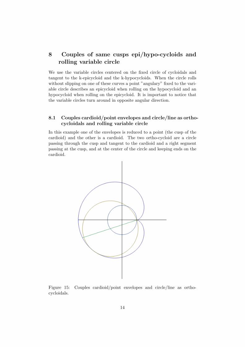
8 Couples of same cusps epi/hypo-cycloids androlling variable circle

We use the variable circles centered on the fixed circle of cycloidals andtangent to the k-epicycloid and the k-hypocycloids. When the circle rollswithout slipping on one of these curves a point ”angulary” fixed to the vari-able circle describes an epicycloid when rolling on the hypocycloid and anhypocycloid when rolling on the epicycloid. It is important to notice thatthe variable circles turn around in opposite angular direction.

8.1 Couples cardioid/point envelopes and circle/line as ortho-cycloidals and rolling variable circle

In this example one of the envelopes is reduced to a point (the cusp of thecardioid) and the other is a cardioid. The two ortho-cycloid are a circlepassing through the cusp and tangent to the cardioid and a right segmentpassing at the cusp, and at the center of the circle and keeping ends on thecardioid.

Figure 15: Couples cardioid/point envelopes and circle/line as ortho-cycloidals.

14

8.2 Couples 2-hypocycloid/nephroid envelope and cardioid/deltoidas ortho-cycloidals and rolling variable circle

Another example is given by the nephroid and the 2-hypocycloid which isthe flat ellipse between the two cusps (a diameter of the fixed circle). Thevariable circle are centered on the fixed circle and tangent to x-axis, its ra-dius is r = sin t. The curve described by a point ”angulary fixed” to thevariable circle rolling without slipping on the diameter is a cardioid (as seenin parag. 3 above) and the curve described similarily by the circle rollingon the nephroid is a deltoid. So it is the couple of curves defined above ascouples of orthogonal curves for rotation around the center O of the fixedcircle. The cardioid constantly passes through the two cups of the nephroid,is tangent to the nephroid and its cusp stays on the 2-hypocycloid (the di-ameter). The deltoid passes through the cusps of the nephroid, is constantlytangent to the diameter and its 3 cusps move on the fixed nephroid. Wehave seen above similar property for a couple of moving cycloids.

8.3 Couples deltoid/3-epicycloid envelopes and nephroid/astroidas ortho-cycloidals and rolling variable circle

The next example is the couple of envelopes (deltoid and 3-epicycloids).One can find on web sites animations [see (8) (9) or (11)] as example of acouple of mirror curve and its caustic by reflection. For light rays comingfrom infinity the caustic by reflection of a deltoid is an astroid and if wechange the direction of the rays this astroid turns inside the two cycloidaleenvelopes.The astroid and the nephroid are the corresponding couple of ortho-cycloidalsand can be generated by a variable circle rolling on these two curves gen-erates a nephroid when rolling on the deltoid and an astroid when rollingon the 3-epicycloid. The nephroid has its cusps on the deltoid an is tangentto an arch of the 3-epicycloid. The astroid has its cusps on the 3-epicycloidand is tangent to an arch of the deltoid. If we change the point by the anglegap t2 on the variable circle all the positions can be obtained and permitto draw animations using only circles with fixed radius as a moving by ro-tation inside the two fixed cycloidals. An alternative animation can use anangulary fixed point on the variable circle.Equations of the two envelope Epi- and Hypo-cycloids (outside (R) andinside (R) of the base circle) are :

X1(t) = R cos t+ 2.r sin[(R/(2r))t]. sin[t ∗ (2r +R)/(2r)]

Y1(t) = R sin t− 2.r sin[(R/(2r))t]. cos[t ∗ (2r +R)/(2r)] (1)

15

X2(t) = R cos t+ 2.r sin[(R/(2r))t]. sin[t ∗ (2r −R)/(2r)]

Y2(t) = R sin t− 2.r sin[(R/(2r))t]. cos[t ∗ (2r −R)/(2r)] (2)

The following curves are the couple the orthocycloidals turning inside thecouple of two cycloidals with same cusps above. Equations of these lociiof a point attached to the variable circle at position tp rolling in oppositerotation repectively on the first couple of Epi-/Hypo-cycloidals envelopesabove are:

X3(t) = R cos t+ 2.r sin[(R/(2r))(t)]. sin[(t− tp) ∗R/(2r)]

Y3(t) = R sin t− 2.r sin[(R/(2r))(t)]. cos[(t− tp) ∗R/(2r)]

X4(t) = R cos t+ 2.r sin[(R/(2r))(t)]. sin[(t− tp) ∗R/(2r)]

Y4(t) = −R sin t− 2.r sin[(R/(2r))(t)]. cos[(t− tp) ∗R/(2r)]

(Nota :The following paragraph needs to be improved)These equations give means to draw all the curves in the figures of this pa-per. The element of arc length of the envelope k-epicycloidal (1) and tangentof the current tangent to the cycloidal are :

ds1 = 2.(R+ r) sin[R

2rt]dt; tan(θ1) = tan[

R+ 2r

2rt]

The element of arc length of the envelope k-Hypocycloidal (2) is :

ds2 = 2.(R− r) sin[R

2rt]dt; tan(θ2) = tan[

2r −R2r

t]

For the rolling variable circle

Rcircle = 2r sin[(R/2r)t]

centered on base fixed circle the element of arc is given by

ds1−circle = Rcircle.dθ1 = (2r +R) sin[(R/2r)t]dt

for rolling on cycloidal (Epi-envelope). The same size circle rolling in theopposite sense

ds2−circle = Rcircle.dθ2 = (2r −R) sin[(R/2r)t]dt

will be used for rolling on cycloidal (Hypo-envelope). So we have the follow-ing formulas :

dθ1 =2r +R

2rdt; ds1−circle = ds1 −R. sin[

R

2rt]dt

16

dθ2 =2r −R

2rdt; ds2−circle = −ds2 +R. sin[

R

2rt]dt

These equations show that the resulting rolling is the composition of a themovement of the center of the variable circle and a rolling of this circlerespectively on the envelope Epi-/Hypo-cycloidals above in the oppositedirection of rotation.

On this example we see that the tangents at cusps are not necessary

Figure 16: Progressive drawing of a the deltoid and cardioid. Orthogonalcardioid and deltoid can turn inside a nephroid. The variable circles rollingon fixed envelopes cycloidals once on the 2-Hypo and once on the nephroidgenerate respectively the cardioid and the deltoid.

orthogonal to the fixed curve (as for the ”roulettes”) because the variationof the radius modifies the trajectory. The rolling of the variable circle isnot exactly similar to the rolling of a constant radius circle. The angleposition on the variable circle varies continuously. And when the pointpasses through the circle with radius zero, the angle position is conserved(there is no angular discontinuity).

9 Final remarks.

This paper was inspired essentially by the two paper [R. Goormaghtigh (3)and J. Boyle (7)], the first author for its investigations on specific propertiesof envelopes of families of circles an the second for the new view on caustics,and specially the theorems 1 ”caustics” and 2 ”envelope theorem”. Theseenvelopes of familes of circles certainly hide many other new properties wait-ing to be discovered.

17

References :(1) Franck Morley - On adjustable cycloidal and trochoidal curves. Ameri-can journal of mathematics Vol 16 No 2(Apri. 1894) pp 188-204(2) Maurice Frechet - ”Sur quelques proprietes de l’hypocycloide trois re-broussements”. NAM 4eme serie t.II (Mai 1902).(3) R. Goormaghtigh - ”Sur les familles de cercles” - NAM 4eme serie, t.XVI (janvier 2016)(4) Walter Wunderlich - Uber Gleitkurvenpaare aus Radlinien. Mathema-tische Nachrichten 20 (Dezember 1959)(5) Peter Meyer - Uber Hullkurven von Radlinien -ARCH. MATH. Vol.XVIII, 1967(6) Jens Gravensen - The geometry of the Moineau pump - Technical uni-versity of Denmark (26 mars 2008)(7) J. Boyle Using rolling circles to generate caustic envelopes resulting fromreflected light - The ArXiv (2014) .(8) http://www.mathcurve.com/courbes2d/astroid/astroid.shtml(9) http://www.vivat-geo.de/zykloidenkette-1.html(10) https://johncarlosbaez.wordpress.com/2013/12/03/rolling-hypocycloids/(11) http://demonstrations.wolfram.com/CausticsGeneratedByRollingCircles/(12) Ernesto Cesaro ”Sur une classe de courbes planes remarquables” NAM1900 - 3eme serie - Tome 19 - p489-494 - Nouvelles annales de mathema-tiques (1842-1927) Archives Gallica.- Journal de mathematiques pures et appliquees (1836-1934) Archives Gal-lica.This paper is the XIV th part on a total of 14 papers on Gregory’s transfor-mation and plane curves.Part I : Gregory’s transformation.Part II : Gregory’s transformation Euler/Serret curves with same arc lengthas the circle.Part III : A generalization of sinusoidal spirals and Ribaucour curvesPart IV: Tschirnhausen’s cubic.Part V : Closed wheels and periodic groundsPart VI : Catalan’s curve.Part VII : Anallagmatic spirals, Pursuit curves, Hyperbolic-Tangentoid spi-rals, β-curves.Part VIII : Translations, rotations, orthogonal trajectories, differential equa-tions, Gregory’s transformation.Part IX : Curves of Duporcq - Sturmian spirals.Part X : Intrinsically defined plane curves, periodicity and Gregory’s trans-formation.Part XI : Inversion, Laguerre T.S.D.R., Euler polar tangential equation andd’Ocagne axial coordinates.Part XII : Caustics by reflection, curves of direction, rational arc length.Part XIII : Catacaustics, caustics, curves of direction and orthogonal tan-

18

gent transformation.Part XIV : Variable rolling circles, orthogonal cycloidal trajectories, en-velopes of variable circles.Part XV : Rational expressions of arc length of plane curves by tangent ofmultiple arc and curves of direction.Part XVI : Logarithmic spiral, aberrancy of plane curves and conics.Two papers in french :1- Quand la roue ne tourne plus rond - Bulletin de l’IREM de Lille (no 15Fevrier 1983).2- Une generalisation de la roue - Bulletin de l’APMEP (no 364 juin 1988).There is an english adaptation.Gregory’s transformation : http://christophe.masurel.free.fr orhttp://christophe.masurel.free.fr/#s9

19