Model Sailing Club Of the Chesapeake Sailing Bay Maritime ...
Upload
vuongthuanCategory
view
222download
2
Ceriotti, Matteo, Harkness, Patrick, and McRobb, Malcolm (2014) Variable-geometry solar sailing: the possibilities of the quasi-rhombic pyramid. In: Macdonald, Malcolm (ed.) Advances in Solar Sailing. Series: Springer Praxis Books: Astronautical Engineering . Springer in association with Praxis Publishing, pp. 899-919. ISBN 9783642349065 Copyright © 2014 Springer A copy can be downloaded for personal non-commercial research or study, without prior permission or charge Content must not be changed in any way or reproduced in any format or medium without the formal permission of the copyright holder(s)
When referring to this work, full bibliographic details must be given
http://eprints.gla.ac.uk/91156/
Deposited on: 13 February 2014
Enlighten – Research publications by members of the University of Glasgow http://eprints.gla.ac.uk

Variable-geometry solar sailing:
the possibilities of the quasi-rhombic pyramid
Matteo Ceriotti,* Patrick Harkness
† and Malcolm McRobb
‡
University of Glasgow, Glasgow, G12 8QQ, United Kingdom
Variable geometry solar sailing potentially offers enhanced delta-V capabilities and
new orbital solutions. We propose a device with such capabilities, based upon an
adjustable quasi-rhombic pyramid sail geometry, and examine the benefits that can be
derived from this additional flexibility. The enabling technology for this concept is the
bevel crux drive, which can maintain tension in the solar sail across a wide range of apex
angles. This paper explores the concept of such a device, discussing both the capabilities
of the architecture and the possibilities opened up in terms of orbital and attitude
dynamics.
I. Introduction
OLAR sails have long been proposed as a mechanism for interplanetary travel [1], using sunlight to
accelerate across space unconstrained by propellant reserves. In more recent years the opportunities that solar
sails provide in terms of highly non-Keplerian behavior, with applications such as displaced orbits [2] and polar
loitering [3], have come to be recognized, and attractive concepts such as orbit raising from low Earth orbit [4]
and inclination change [5] have been proposed.
To achieve these objectives, some form of control over the direction and magnitude of the thrust produced by
the solar sail has usually been required [6]. It has been suggested that the solar sail can be tilted, using masses or
propellant, as part of an active attitude and orbit control system [7] and that the thrust vector could be modified
by changing the reflectivity of the membrane [8].
However it is now proposed that, in some cases, management of both the direction and magnitude of the
thrust vector could be achieved without resorting to the use of propellant, control masses and exotic membranes
equipped with liquid crystals or e-ink. This could be done by combining a “heliostable” solar sail, which is to say
* Lecturer, School of Engineering, James Watt Building South. Tel: +44 141 330 6465. Email:
[email protected] † Lecturer, School of Engineering, James Watt Building South. Tel: +44 141 330 3233. Email:
[email protected] ‡ Research Assistant, School of Engineering, James Watt Building South. Tel: +44 141 330 2477. Email:
S
a shape that, when deflected, produces a restoring moment back towards he sun, with a geometry that can vary
the apparent size and inclination of the solar sails without rotation of the bus.
Such a geometry might be realized in a quasi-rhombic pyramid (QRP), in which the spacecraft bus would lie
at the apex and deploy booms along the slant edges, with the membranes filling the slant faces. By considering
the four booms to be arranged in two opposing pairs, and starting in the degenerate case of a square-based
pyramid, it is apparent from Fig. 1 that increasing the flare angle of one opening boom pair (orange arrows) and
simultaneously reducing the flare angle of the other closing pair (blue arrows) will serve to reduce the area
presented to the sun without creating any net torque about the apex. Provided that the angular positions of the
opening and closing pairs are carefully matched, the membrane will remain taut and the heliostable behavior will
be maintained throughout, albeit to diverging extents in the two orthogonal planes.
This paper seeks to outline the capability that such variable-geometry solar sailing could provide to nanosat-
sized spacecraft operating in near-Earth space. Deploying sail-like structures from a nanosats can be done [9],
but most architectures offer only a simple deploy-and-forget behavior similar to that provided by the commercial
AEOLDOS module. In these cases, multiple booms are often spooled around a shared hub to reduce complexity
and provide some measure of mutual support.
We therefore propose a new mechanical arrangement, the bevel crux drive (BCD), that builds on traditional
deployment concepts but which provides the flexibility required to vary the boom angles independently after
deployment. This is achieved by deploying each boom from its own dedicated spool, the spool rotating when
released due to strain energy stored in the deflected boom itself. Each boom is deployed tangentially to the spool
and is constrained by a cage of roller bearings, as has been proposed elsewhere [10], with mutual support
between the spools now being provided by linking each to its neighbors through a simple arrangement of bevel
gears. After the deployment is complete the spools become fixed but each circumferential cage of roller bearings
is permitted to rotate about its host spool over a short angular distance. This permits independent pointing of
each deployed boom.
The BCD arrangement has an additional advantage in that, in contrast to some similar deployment
architectures [11], the deployed sails exhibit perfect radial symmetry. This means that fold patterns can be
simplified, which facilitates packing, and the potential for significant out-of-plane forces that could tend to
buckle the booms during deployment is reduced.
This paper investigates these factors in some detail and goes on to consider how a QRP-sail might be used to
raise the orbit of a small satellite in LEO. We suggest that the solar sail could be opened such that the solar

radiation pressure may provide an accelerating force as the satellite moves away from the sun and then closed to
minimize the braking force as it moves towards the sun in the second half of the orbit, the heliostable behavior
and onboard dampers keeping the apex pointed approximately towards the SRP vector throughout.
Fig. 1 The quasi-rhombic pyramid concept.
II. Geometry and mass properties
This paper will consider that the booms have already fully deployed, and all the analyses will be done in this
configuration. We assume the (extended) booms have the same length, which is set to l. Since the sail membrane
must be always tensioned, the size of each triangular face of the QRP cannot be altered. This means that the
distance between any two adjacent boom tips (e.g. A and B) is constant and set to b , see Fig. 2 (which also
shows the body axes).
Fig. 2 One face of the QRP, in two different configurations. Highlighted are the body axes and the planes
x-z and y-z in which the two booms move.
O
y x
z
B A b
l
b a
l
O
y x
z
B b
b a
l A
l
QRP face
(reflective sail membrane)
QRP apex with BCD mechanism
(sun-pointing)
Spacecraft bus
Booms

The area of each triangular face, which can be computed through Heron’s formula, is:
2 24
4
bS l b
The control of the sail is done by varying the flare angle of the booms with respect to the spacecraft body
axis z. Because of symmetry, opposite booms must have the same flare angle at all times, hence we can consider
the angles of the two adjacent booms, ,A B . Referring to Fig. 2, the Cartesian coordinates in body frame of
their tips A and B are functions of these angles:
sin 0
0 ; sin
cos cos
A
A B B
A B
l l
r r (1)
By writing the expression for the Cartesian distance between A and B, setting it equal to b and squaring:
2 22 2sin sin cos cosA B A Bb l
Assuming boom A is the driver, and boom B is driven, we can derive an expression that defines the flare
angle of B, for any flare angle of A, in order to maintain the sail tension:
22
arccos2cos
B
A
b l
(2)
The maximum value for b/l is clearly 2 , such that both A and B are acute. In such case, each face is an
isosceles right triangle. All four booms have the same flare angle when A B , or:
2
,
2cos
2A B
b l
(3)
Taking the (time) derivative of Eq. (2), allows to find the gear ratio to connect the driver booms to the driven
booms:
2
2
22
22
2
sin 2
2
2cos 14cos
A
B A
A
A
b
l
b
l
(4)
Equation (2) also gives a maximum value for the angle of the driver boom A, which is obtained when the
driven boom B is fully closed, i.e. 0B . With this condition, we can write (for both boom A and B):
2
,
2arccos
2A B
b l

In the particular case of equilateral face ( l b ), the maximum angle of the booms is 3 , while in the
(limit) case where 2b l , then from Eq. (2), 2B , so the driven boom B is always fully open, regardless
of the position of the driver boom A.This corresponds to a square sail that folds along the diagonal.
Fig. 3 shows the relations between angular positions [Eq. (2)] and angular velocities [Eq. (4)] between two
adjacent booms, for different values of b l . Note that when 2b l , one set of booms is not moving, but it is
constantly deployed at 90 deg, and the sail folds along the diagonal of a square.
a) b)
Fig. 3 a) θB as function of θA for different values of b/l. b) Derivative (angular velocity of one boom with
respect to the other one).
With no loss in generality, let us consider face AOB. The normal to the face, pointing outwards, is:
ˆ B A
AOB
B A
r rn
r r
The centroid of the face, which is also the geometric barycenter, is simply the average of the three vertices:
,
1
3CM AOB A B O r r r r (5)
Three different sail configurations, varying the flare angles of the booms, are represented in Fig. 4.
a) b) c)
Fig. 4. Sail configurations for b = l = 1: a) θa = 5 deg; a) θa = 55 deg (maximum effective area); c) θa = 55
deg. Face normal and principal axes of inertia are also represented.

A. Mass properties
If we consider a uniform areal density of the sail material, then this point coincides with the center of
mass of the face. The value of however shall take into account an average density that considers the mass of
the booms. So for a square sail with X-type booms, the equivalent , considering a membrane of mass per unit
area membane and booms of mass per unit length
boom , is:
4 4
4
membane boomS l
S
The mass of the spacecraft has two contributions: one due to the QRP sail assembly and one due to the
spacecraft bus. The bus is considered to be a point mass at (0,0,0) with mass busm and moments of inertia
busI ,
with respect to its own center of mass:
4 busm S m
The center of mass of the whole spacecraft is then:
4
,
1
CM i
i
CM
S
m
r
r
It can easily be shown that , , 0CM x CM yr r , and this will be used for computing the moments of inertia.
B. Moments of inertia
1. Sail face
Due to symmetries, the principal axes of inertia are aligned with the body axes x, y, z in any configuration of
the spacecraft. The moment of inertia of one sail face (e.g. AOB), is:
2
AOBS
I d dS r (6)
where d r is the distance of the point to the considered axis of inertia. The integration domain S is the
triangular sail surface.
Let us introduce a parameterization of the surface ,s t where s is along the edge and t is parallel to the base
(see Fig. 5). The infinitesimal area of each surface element then becomes:
cosdS dtds dt ds
where the angle arcsin 2b l . Equation (6) can be re-written as:
2
0 0cos
bl s
lAOBI d dtds (7)

where 2
2cos 1
4
b
l . To compute the distance of each point on the face to one of the axes, we shall compute
the coordinates of the generic point R on the triangle:
sin sin
0 sin
cos cos cos
A A
Q P
R P B
A B A
lt s t
bPQ
r rr r
The distance of R to the three principal axes of inertia is then:
22 2
, , ,
22 2
, , ,
2 2 2
, ,
x R y R z CM z
y R x R z CM z
z R y R x
d r r r
d r r r
d r r
The integral in Eq. (7) is then polynomial in s, t and can be computed analytically, for given flare angles of
the booms.
Fig. 5 Parameterization of the sail face.
2. Overall spacecraft
Due to symmetry, each face contributes in the same way to the moment of inertia of the spacecraft about
each principal axis. The principal moments of inertia for the whole spacecraft are then:
2
, , ,
2
, , ,
, ,
4
4
4
x x AOB bus CM z bus x
y y AOB bus CM z bus y
z z AOB bus z
I I m r I
I I m r I
I I I
(8)
where busI are the components of the principal moments of inertia of the spacecraft bus with respect to its own
center of mass [assumed in (0, 0, 0)]. Considering a uniform cube of side busl :
2
, , ,6
bus bus
bus x bus y bus z
m lI I I
C. Forces and torques
The net force generated by solar radiation pressure (SRP) in ideal conditions, on each face i, is [12]:
x
y
O
b
P
Q
R
l
b
R
P
s
t
ds
dt
dh
Plane of the face

2
ˆ ˆ ˆ2i sun i s iP S f n r n (9)
in which sr is the sun vector, representing the direction of the sun in the same reference frame (body axes), and
sunP is the SRP of the sun, which varies as 21 sr and at 1 AU is approximately 4.56 x 10⁻⁶
N/m2. is the
efficiency of the solar sail material in terms of reflectivity, ranging from 0.5 (full absorption) to 1 (full specular
reflection). Note that diffraction and other effects are not explicitly considered here, but embedded in the
efficiency . The force if is only experienced on a face, if the face is lit by the sun, i.e. ˆ ˆ 0i s n r . If not, then
the face does not provide force and it is not taken into account. The total acceleration experienced by the
spacecraft, considering all four faces, is simply the sum of the forces on each face:
4
1
1sail i
im
a f (10)
Similarly, given the position C of the center of mass of the spacecraft, the total torque about that point is:
4
,
1
CM i CM i
i
t r r f (11)
III. Mechanical layout
The solar sail is extended in a largely-passive deployment phase, during which each section of the sail is
extended from its stowage volume by the booms on either side; and subsequently articulated, for the remainder
of the mission, in an active control phase during which the booms are pivoted about their inboard end.
The deployment phase is a mechanical process that uses a four-boom BCD assembly powered by strain
stored in the booms themselves. Subsequently, in the active control phase, the flare angle of each boom may be
varied either independently or collectively using one of three proposed electromechanical techniques to position
the cage of roller bearings that surrounds each spool. The complexity of these electromechanical processes
varies, but each presents its own advantages and disadvantages.
A. Deployment Phase
The BCD is a novel gearing architecture that communicates torques generated by tape spring booms through
a series of bevel gear subassemblies arranged in a closed loop, thus providing mutual support, shared momentum
and mechanical synchronization between the four spool assemblies.
Although the present work considers a four-boom case, due to the specific requirements of the quasi-rhombic
pyramid solar sail, the BCD is a highly flexible architecture that can accommodate multiple booms and thus
approximate a cone if required. Fig. 6 illustrates that, provided that the pitch cone angles and subassembly

spacings remain equal around the loop, the relationship between the number of booms and the pitch cone angle is
expressed by 360 2boom coneN , where boomN is the number of booms arrayed radially and
cone is the pitch
cone angle of each bevel gear.
Fig. 6 BCD configurations showing the number of bevel subassemblies with associated pitch cone angles
required.
B. Active Control Phase
During deployment, the booms extend tangentially away from their spools and a circumferential cage of
roller bearings around each spool is used to control the direction of the tangent. These cages remain fixed during
deployment to ensure that the booms extend with a common flare angle, but in the active control phase the cages
may be rotated about their spools. As is shown in Fig. 7, this means that the flare angle of each boom can be
adjusted independently.
Fig. 7 Variable pitch capability provided by rotating a cage structure about a single spool of the BCD.
Assembling four spool-and-cage units into a BCD layout provides the mechanical basis for the deployment
of the quasi-rhombic pyramid from a realistic CubeSat module. Such a device is represented in Fig. 8a, where
the yellow booms (in this case, tape-springs) are deployed from purple spools and directed by blue roller
bearings in green cages. Fig. 8b shows a physical prototype of this concept, which was approximately 0.6U and
which successfully deployed a Mylar membrane against gravity in laboratory conditions.

a) b)
Fig. 8 a) Preliminary concept of the BCD in a 4-boom configuration. b) First technology demonstrator of
the BCD in a 4-boom configuration.
C. Articulation
Three specimen articulation methods are explored, namely independent stepper motors for each cage, two
stepper motors each linked to a pair of cages, and a single stepper motor mechanically linked to all four cages.
1. Independent Stepper Motors
By employing the approach depicted in Fig. 9a, the flare angle of each boom may be controlled
independently via a stepper motor and worm gear engaging with teeth fabricated into the roller cage. Algorithms
will be necessary to control each stepper motor and thus ensure that all four booms move in a manner that
maintains the desired global shape. This approach has the advantage that, at the end of the deployment phase, the
sail need not come under any undue stress because the booms may be arranged such that all the membrane
quadrants are initially slack. This could reduce the risk of tearing, with tension subsequently being applied in a
controlled fashion via the stepper motors.
2. Paired Stepper Motors
The number of stepper motors may be halved by appropriately linking each opposing pair of cages, in
compliance with the global behaviour of the quasi-rhombic pyramid, through a shaft driven by a single motor.
The control algorithm is still required to match the speed of the two shafts, and a stress-relieving procedure at
end-of-deployment is still possible. To ensure that both booms in each set rotate in the correct direction from one
another when the controlling motor turns either clockwise or anticlockwise it would be necessary to use both a
lefthand and a righthand driven worm gear in each set, as indicated by Fig. 9b.
3. Single Mechanically Linked Stepper Motor
It may be possible to eliminate all but one motor by performing the matching function of the control
algorithm with a mechanical device such as an elliptical gear train [13]. Fig. 9c shows a schematic of one such

approach, using a combination of bevel and elliptical gears to transmit motion from a single motor to all four
worm gears. It should be noted that full rotations are not required in the current architecture and so the elliptical
gears do not have to achieve full rotations in this case. The elliptical gear ratio is given in Eq. (4).
a) b) c)
Fig. 9 a) one motor per cage; b) one motor per pair of cages; and c) a single motor for all four cages.
IV. Spacecraft data
For the simulations shown later in this paper we will use three spacecraft, which differ in dimensions and
masses, corresponding to three different levels of technology. The data presented in Table 1 is common to the
three, but Table 2 presents dimensions, masses and other quantities that change between the spacecraft models.
By using the formulas in Section II, it is possible to compute the values in Table 3, which essentially characterize
each individual spacecraft.
As will be explained in detail in a later section, the control law requires two different configurations: one in
which the driver booms are fully closed and one in which the booms are fully open (the transition between the
two configurations is not considered). In the “closed” configuration, we consider 5A , while in the “open”
configuration, the booms are such that A B , according to Eq. (3), and the frontal sail area is maximized.
Table 1 Common spacecraft data
membrane , g/m2 13.2
boom , g/m
16.3
Efficiency of the sail, 0.85
Table 2 Specific spacecraft data
Spacecraft 1 2 3
Boom length, l, m 1 2 3
QRP base length, b, m 1 2 3
Bus mass, busm , kg 1 2 3
Bus size, busl , cm 10 12.6 14.4
Rotational damping coefficient, c, Nm/rad s 61 10 64 10 84 10
Sail assembly mass per unit area, , kg/m2 0.050 0.032 0.026

Table 3 Computed data
Spacecraft 1 2 3
Total mass, m, kg 1.088 2.221 3.401
Equivalent flat sail area-to-mass ratio, *
eqAMR , m2/kg
(booms open) 0.001 0.002 0.003
Equivalent flat sail area-to-mass ratio,*
eqAMR , m2/kg
(booms closed) 0.30 0.60 0.88
Moment of inertia of the damping fluid, *
fI , kg m2 41.25 10 43.97 10 47.80 10
Principal moments of inertia, I, kg m2 (booms open)
0.0294
0.0294
0.0163
0.281
0.281
0.153
1.120
1.120
0.612 * See following Sections V and VI for definition.
V. Attitude motion
In this section and in the following, simulations of the attitude motion and orbital motion will be presented.
Although the two types of motion are in fact simultaneous, for the sake of this simulation we assume that the
spacecraft deploys the sail, stabilizes itself in terms of attitude, and then begins the analyzed orbit. In this way,
we can consider the orbital motion as being not affected by initial attitude changes.
One of the advantages of the QRP sail is its equilibrium position, under SRP, with the tip pointing towards
the sun. An angular displacement from this position results in a heliostable torque in the opposite direction (see
Fig. 10) which, if undamped, essentially provides an elastic oscillation about the equilibrium position.
Fig. 10 Sun-pointing effect.
Damping can be obtained with a pair of fluid dampers, one for each body axis x and y, of the type used on
spun spacecraft for nutation damping. They usually consist of a sealed ring attached to the spacecraft bus, filled
with a viscous fluid. When the spacecraft experiences an angular acceleration in the direction perpendicular to
the ring, a difference in angular velocity between the fluid inside the ring and the ring walls is created, which
causes viscous friction and therefore dissipates rotational energy as heat.

Fig. 11 Annular damping fluid rings (yellow).
The differential equations of motion of the fluid in each ring can be written considering that the fluid is
accelerated by viscous effects which depend on the relative velocity between the fluid itself and the ring. Named
, ,,f x f y the (average) velocity of the fluid in each ring, and ω the angular velocity of the spacecraft in body
axes, we can write:
,fx x fy y
fx fy
f f
c c
I I
(12)
where c is a coefficient that depends on the fluid viscosity and fI is the moment of inertia of the fluid in the
ring. Considering a ring whose radius is half of the spacecraft bus side (see again Fig. 11), and which has a mass
1/20 of the spacecraft bus mass, we have 2
20 2f bus busI m l .
The dynamical equation for the angular velocity in body axes ω of the spacecraft can now be derived. They
are essentially the classic Euler equations, combining the fluid rings and the rest of the spacecraft:
x x z y z y f fx f z fy x
y y x z x z f fy f fx z y
z z z y z y f x fy f fx y z
I I I I I t
I I I I I t
I I I I I t
(13)
The SRP torque t is computed in Eq. (11) and matrix of inertia I, in principal inertia axes, in Eq. (8). Equations
(12) can be solved for ,fx fy , and these values substituted in Eqs. (13). Equations (12) and (13) can therefore
be integrated in time to determine the attitude motion of the spacecraft under SRP.
It is possible to show that there is an optimal value for the fluid coefficient, c, to maximize the damping
action, and that this value depends on the moments of inertia of the spacecraft. In essence, a small value of c will
result in a negligible acceleration of the fluid within one period of the oscillation, while a great value of c will
y
x
2busl
busl

result in a fluid that is almost rigidly connected with the ring walls. In either case, the damping action is
diminished.
Attitude parameterization is performed with quaternions [14]. A quaternion q defines the attitude of the body
reference frame with respect to the inertial one. The dynamics of the quaternions can be expressed as a function
of the angular velocity ω in body axes ,q q ω q (see Ref. [14], pp. 104-110), and this equation can therefore
be integrated over time, together with the Euler equations (13). The attitude parameterization is used to compute
the direction of the sun ˆsr in body axes, as required in Eq. (9). In general, from the quaternions, it is possible to
compute the direction cosine matrix as A A q , and therefore we obtain the sun vector in body axes,
ˆ ˆ ECI
s sr Ar . The superscript (ECI) denotes an inertial frame (and we assume the direction of the sun is known
and fixed in this frame), e.g. Earth-Centered Inertial. For the sake of the attitude simulation, we can arbitrarily
choose ˆ 0 0 1
TECI
s r .
A. Results
Results are presented here for each one of the three spacecraft in the open configuration. The spacecraft
initial position is rotated of an angle of 30 deg around its y axis, and the initial angular velocity of the spacecraft
(and the fluid dampers) is initially zero. The damping effect is different on the three spacecraft due to their
various moments of inertia, which differ by about one order of magnitude each time (see Table 3). For spacecraft
1, after about 60 hours the amplitude of the oscillations is reduced to about 3 deg, and this is considered a
sufficient pointing accuracy (see Fig. 12a, which represents the angular velocity of the spacecraft and the
damping fluid). A closer inspection to the first periods of the motion (see Fig. 12b) highlights the velocity of the
spacecraft with respect to the fluid: their difference is related to the instantaneous dissipation. For spacecraft 2
and 3, the dissipation becomes less and less effective: after 6 days, the amplitude of the oscillations is about 5
deg and 15 deg respectively. For reference, the torque experienced by each spacecraft at 30 deg tilt are:
-1.50×10⁻⁶
, -1.18×10⁻⁵
, -3.94×10⁻⁵
Nm2 respectively.

a) b)
Fig. 12 Angular velocity of spacecraft and damping fluid for spacecraft 1 on initial displacement of 30 deg
in y. a) 6 hours; b) a magnification of the first hour.
With the selected initial conditions, and since the y axis is a principal axis, no motion around x is involved. A
coupled movement can be obtained by initiating the simulation with the spacecraft rotated around an arbitrary
axis, for example [0.5, 0.866, 0]T. This case, for spacecraft 1, is represented in Fig. 13, which shows how both
annular dampers are effective. Although it is not visible from the figure, the damping time is very similar to the
previous case.
Fig. 13 Angular velocity of spacecraft and damping fluid for spacecraft 1 on initial displacement of 30 deg
around axis [0.5, 0.866, 0].
VI. Orbital motion
For the orbital motion of the spacecraft we consider the action of the gravity of the Earth (considered a point
mass with planetary constant 5 3 -23.986 10 km s ) and the effect of SRP.
Given the heliostable behavior of the spacecraft explained above, we consider the orbital simulation when
the attitude transient phase is concluded and the spacecraft is in an equilibrium attitude with the tip of the sail
towards the sun. This attitude is maintained in an inertial, Earth-centered reference frame, while the sun direction

rotates around the Earth, so with a period of one year the equilibrium attitude of the spacecraft will execute a
complete revolution.
Under this scenario, the net force experienced by the spacecraft due to SRP can be thought as one given by a
flat sail, facing the sun, of the same efficiency and equivalent area 4
1
2eq i sun
i
AMR P m
f (see again Table
2).
The differential equation of motion of the spacecraft is:
2ˆ ˆECI ECI ECI
sail sar
r r r (14)
where r is the position vector in an Earth-centered, equatorial inertial (ECI) reference frame and saila is the
magnitude of the acceleration due to SRP computed in Eq. (10). The direction is opposite to the direction of the
sun, as explained.
The direction of the Sun, in ECI and as function of time, assuming a circular Earth orbit around the sun, is
given by [15]:
0
ˆ cos sin cos sin sin ,TECI
s t r
where is the longitude of the sun, is the angular velocity of the Earth around the sun (assumed constant at
one revolution per year), and 23.5 is the obliquity of the equator on the ecliptic plane. By choosing 0 0 ,
then at time 0t the sun is at the vernal equinox in the equatorial plane.
Due to the small perturbing acceleration with respect to the gravitational acceleration, the Keplerian elements
of the orbit , , , ,a e i (apart from the true anomaly f ) change very slowly. For this reason, the integration is
performed using Gauss’ variational equations (Ref. [16], pp. 488-489). In this formulation, the perturbing
acceleration saila is decomposed in tangential ˆ ˆt v , normal n and out-of-plane direction h , with respect to the
orbital plane (tnh). This can be obtained through the rotation matrix ˆˆ
B v n h from ECI system to tnh, as
ˆtnh ECI ECIT T
sail sail sail sa a B a B r .
A. Control law
When the sun direction is aligned with the pyramidal axis, the sail acceleration naturally depends on the
length of the booms l and b, but also depends on the instantaneous angle of the booms. Thus, varying the angle
of the booms, according to the law in Eq. (2), can be used to change the acceleration experienced by the
spacecraft. Indeed, we consider that the spacecraft can control the driver boom angle to toggle between two

values, one in with the boom is fully closed, and the other where the four booms are open to the same angle,
according to the value found in Eq. (3). In the former case, the effective area exposed to the sun (and hence the
acceleration) is minimized, in the latter maximized (see Fig. 4).
We now consider control laws that can either increase or decrease the semi-major axis. By inspecting the
Gauss’ equation for semi-major axis it can be seen that, for a maximum change, the sail acceleration shall be
tangential. However, the direction of the acceleration in an ECI frame cannot be arbitrarily decided, being
always pointing away from the sun. Therefore the switching timing between one configuration or the other can
be used as control law.
To increase the semi-major axis, the sail shall be open when the spacecraft is travelling away from the sun,
i.e. ˆ ˆ 0s r v . If the sun is in the same plane of the orbit, then there will be one true anomaly in which ˆ ˆ,sr v are
antiparallel, and thus the only acceleration is tangential. In the other parts of the orbit, it will have a normal
component. If the sun is out of the orbital plane, then there will always be an out-of-plane acceleration
component. When ˆ ˆ 0s r v , the open sail can still provide a (small) contribution to the tangential acceleration,
but there will be major normal and out-of-plane components that will not contribute to the semi-major axis
change. For this reason, it is decided to open the sail when the following condition is verified:
ˆ ˆarccos s control r v
where the angle 0, 2control can be arbitrarily selected. On the lower end of the interval, the spacecraft
receives a quasi-tangential acceleration, but for a limited fraction of the orbit, if any depending on the position of
the sun; on the upper end, the spacecraft maximizes the tangential acceleration, but it experiences a considerable
amount of other components as well. Research has also investigated optimal values for control [17], however
their application is beyond the scope of this paper. The value selected is 80control , which offers a substantial
increase in semi-major axis and very small changes of the other elements. This will result in a control law similar
to what is proposed in Ref. [18] for deorbit, by varying the effective area exposed to SRP by changing the pitch
of the solar panels.
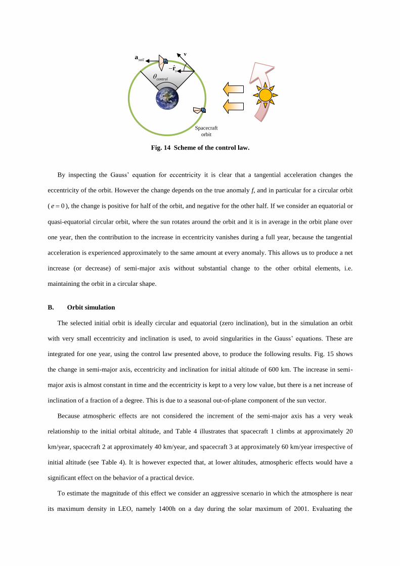
Fig. 14 Scheme of the control law.
By inspecting the Gauss’ equation for eccentricity it is clear that a tangential acceleration changes the
eccentricity of the orbit. However the change depends on the true anomaly f, and in particular for a circular orbit
( 0e ), the change is positive for half of the orbit, and negative for the other half. If we consider an equatorial or
quasi-equatorial circular orbit, where the sun rotates around the orbit and it is in average in the orbit plane over
one year, then the contribution to the increase in eccentricity vanishes during a full year, because the tangential
acceleration is experienced approximately to the same amount at every anomaly. This allows us to produce a net
increase (or decrease) of semi-major axis without substantial change to the other orbital elements, i.e.
maintaining the orbit in a circular shape.
B. Orbit simulation
The selected initial orbit is ideally circular and equatorial (zero inclination), but in the simulation an orbit
with very small eccentricity and inclination is used, to avoid singularities in the Gauss’ equations. These are
integrated for one year, using the control law presented above, to produce the following results. Fig. 15 shows
the change in semi-major axis, eccentricity and inclination for initial altitude of 600 km. The increase in semi-
major axis is almost constant in time and the eccentricity is kept to a very low value, but there is a net increase of
inclination of a fraction of a degree. This is due to a seasonal out-of-plane component of the sun vector.
Because atmospheric effects are not considered the increment of the semi-major axis has a very weak
relationship to the initial orbital altitude, and Table 4 illustrates that spacecraft 1 climbs at approximately 20
km/year, spacecraft 2 at approximately 40 km/year, and spacecraft 3 at approximately 60 km/year irrespective of
initial altitude (see Table 4). It is however expected that, at lower altitudes, atmospheric effects would have a
significant effect on the behavior of a practical device.
To estimate the magnitude of this effect we consider an aggressive scenario in which the atmosphere is near
its maximum density in LEO, namely 1400h on a day during the solar maximum of 2001. Evaluating the
Spacecraft
orbit
v
ˆsr
control
saila

dynamic pressure in a circular equatorial at 600 km, 800 km and 1000 km, and comparing these values to the
solar radiation pressure, we find that the aerodynamic pressure is over 12 times higher at 600 km, falling to 1.3
times higher at 800 km, and only 0.2 times as much at 1000 km. We therefore expect that actual altitude gains
would tend towards the values presented in Table 4 above approximately 1000 km, but are aware that a much
more complex behavior must be expected at lower altitudes. This is due not only to the competing forces but also
to the destabilizing effects of the competing aerodynamic and SRP torques [19].
Finally, we note that altitude reduction, as a part of an end-of-life deorbit scheme, may also be an attractive
application. Under these circumstances a different control law would be required to reduce the semi-major axis,
and it can be envisioned that the heliostable behavior might be exploited above 1000 km and the aerostable
behavior below approximately 600 km, depending on the solar activity. The behavior in the altitude band where
aerodynamic and solar radiation pressures are comparable would naturally be more complex but it is worth
noting that, if sufficient pointing capability is available, relatively early compliance with the aerodynamic vector
may be attractive. This would enable best use of the solar radiation pressure to be made around 0600h, when it is
most effective, and best use to be made of the dynamic pressure around 1400–1600h, when that effect is
strongest. This approach would be further supported by silvering the front surface of the sail to maximize the
solar radiation force in the morning, and blackening the rear surface to minimize the force in the afternoon.
a) b) c)
Fig. 15 Change in a) semi/major axis, b) eccentricity, and c) inclination during one year, starting from
circular equatorial orbit at 600 km altitude.
Table 4 Altitude after one year (km).
Initial
altitude,
km
1 2 3
600 620.7216 640.7249 659.9745
800 821.6338 842.4915 862.5775
1000 1022.551 1044.2801 1065.216
1200 1223.4786 1246.098 1267.896

VII. Conclusions
A new concept of quasi-rhombic pyramid (QRP) solar sail for nanosatellites was explored. The spacecraft
bus, at the apex of the pyramid, deploys booms along the slant edges, with the membranes filling the slant faces.
The enabling technology of the QRP is the bevel crux drive (BCD) mechanism, which allows the deployment
of the quasi-rhombic pyramid sail from a realistic CubeSat-class spacecraft, and to vary the boom angles
independently after deployment.
The QRP shape provides a passive, self-stabilizing effect under solar radiation pressure, such that the apex of
the pyramid will always point to the sun. In addition, by varying the boom angles, it is possible to change the
effective area-to-mass ratio of the spacecraft for orbit control. Although aerodynamic effects may be significant
below approximately 1000 km, realistic architectures appear likely to have the capability to raise the orbit of
CubeSat-class spacecraft above this altitude by several tens of kilometers per year.
References
[1] Tsu, T. C., “Interplanetary Travel by Solar Sail,” ARS Journal, Vol. 29, 1959, pp. 422-427.
[2] Heiligers, J., Ceriotti, M., McInnes, C. R. and Biggs, J. D., “Displaced Geostationary Orbit Design Using Hybrid
Sail Propulsion,” Journal of Guidance, Control, and Dynamics, Vol. 34, No. 6, 2011, pp. 1852-1866.
doi: 10.2514/1.53807
[3] Ceriotti, M. and McInnes, C. R., “Generation of Optimal Trajectories for Earth Hybrid Pole-Sitters,” Journal of
Guidance, Control, and Dynamics, Vol. 34, No. 3, 2011, pp. 847-859.
doi: 10.2514/1.50935
[4] Mengali, G. and Quarta, A. A., “Near-Optimal Solar-Sail Orbit-Raising from Low Earth Orbit,” Journal of
Spacecraft and Rockets, Vol. 42, No. 5, 2005, pp. 954-958.
doi: 10.2514/1.14184
[5] Stolbunov, V., Ceriotti, M., Colombo, C. and McInnes, C. R., “Optimal Law for Inclination Change in an
Atmosphere through Solar Sailing,” Journal of Guidance, Control, and Dynamics, in press.
doi: 10.2514/1.59931
[6] Macdonald, M. and McInnes, C. R., “Analytical Control Laws for Planet-Centred Solar Sailing,” Journal of
Guidance, Control, and Dynamics, Vol. 28, No. 5, 2005, pp. 1038-1048.
doi: 10.2514/1.11400
[7] Wie, B. and Murphy, D., “Solar-Sail Attitude Control Design for a Flight Validation Mission,” Journal of Spacecraft
and Rockets, Vol. 44, No. 4, 2007, pp. 809-821.
doi: 10.2514/1.22996
[8] Wie, B., “Solar Sail Attitude Control and Dynamics, Part 1,” Journal of Guidance, Control, and Dynamics, Vol. 27,
No. 4, 2004, pp. 526-535.

doi: 10.2514/1.11134
[9] Johnson, L., Whorton, M., Heaton, A., Pinson, R., Laue, G. and Adams, C., “Nanosail-D: A Solar Sail
Demonstration Mission,” Acta Astronautica, Vol. 68, No. 5-6, 2011, pp. 571–575.
doi: 10.1016/j.actaastro.2010.02.008
[10] Shmuel, B., Hiemstra, J., Tarantini, V., Singarayar, F., Bonin, G. and Zee, R., “The Canadian Advanced Nanospace
Experiment 7 (Canx-7) Demonstration Mission: De-Orbiting Nano- and Microspacecraft,” 26th AIAA/USU Small
satellite conference, USA, 2012.
[11] Lappas, V., Adeli, N., Visagie, L., Fernandez, J., Theodorou, T., Steyn, W. and Perren, M., “Cubesail: A Low Cost
Cubesat Based Solar Sail Demonstration Mission,” Advances in Space Research, Vol. 48, No. 11, 2011, pp. 1890-
1901.
doi: 10.1016/j.asr.2011.05.033
[12] McInnes, C. R., Solar Sailing: Technology, Dynamics and Mission Applications, Springer-Praxis Books in
Astronautical Engineering, Springer-Verlag, Berlin, 1999.
[13] Litvin, F. L., Gonzalez-Perez, I., Fuentes, A. and Hayasaka, K., “Design and Investigation of Gear Drives with Non-
Circular Gears Applied for Speed Variation and Generation of Functions,” Computer Methods in Applied Mechanics
and Engineering, Vol. 197, No. 45–48, 2008, pp. 3783-3802.
doi: 10.1016/j.cma.2008.03.001
[14] Schaub, H. and Junkins, J. L., Analytical Mechanics of Space Systems, 2nd Edition Aiaa Education Series, Reston,
VA, USA 2009.
[15] Krivov, A. V., Sokolov, L. L. and Dikarev, V. V., “Dynamics of Mars-Orbiting Dust: Effects of Light Pressure and
Planetary Oblateness,” Celestial Mechanics and Dynamical Astronomy, Vol. 63, No. 3-4, 1995, pp. 313-339.
doi: 10.1007/bf00692293
[16] Battin, R. H., An Introduction to the Mathematics and Methods of Astrodynamics, Revised edition, Aiaa Education
Series, AIAA, New York, 1999.
[17] Gao, Y., “Near-Optimal Very Low-Thrust Earth-Orbit Transfers and Guidance Schemes,” Journal of Guidance,
Control, and Dynamics, Vol. 30, No. 2, 2007, pp. 529-539.
doi: 10.2514/1.24836
[18] Borja, J. A. and Tun, D., “Deorbit Process Using Solar Radiation Force,” Vol. 43, No. 3, 2006, pp. 685-687.
doi: 10.2514/1.9508
[19] Harkness, P. G., “An Aerostable Drag-Sail Device for the Deorbit and Disposal of Sub-Tonne, Low Earth Orbit
Spacecraft,” Cranfield University, Cranfield, UK, 2006.