VARIABILITY OF FORMANT MEASUREMENTS

by

Philip Harrison

Submitted in partial fulfilment of the degree

of MA at the department of

Language and Linguistic Science, University of York

Word Count: 13,382

VARIABILITY OF FORMANT MEASUREMENTS

by

Philip Harrison

September 2004

Supervisor: Dr Paul Foulkes

Submitted in partial fulfilment of the degree

of MA at the department of

Language and Linguistic Science, University of York

i

Foreword

This dissertation was submitted in September 2004 as part of my MA course in

Phonetics & Phonology at the Department of Language and Linguistic Science at

the University of York, England. Having gained a Distinction for this work, I am

currently embarking on a PhD within the same department. This will expand on

and progress the work described herein. My intention is to further investigate

some of the factors which affect formant measurements. In the first instance, I

will reanalyse the formant data, as well as analysing the material from the

telephone recordings. At present, the other areas of investigation have not been

finalised. However, possibilities under consideration are the effects of GSM

coding/transmission, the effects of mouth-telephone distance, acoustic

environment and recording circuitry.

Please feel free to contact me with any comments or suggestions which arise

from reading this dissertation.

If you have a serious interest in analysing any of this material from a different

angle, please let me know. It might, under certain circumstances, be possible to

provide you with copies of the recordings and/or the formant data.

Philip Harrison

pth@jpfrench.com

February 2006

ii

Abstract

One of the main types of analysis conducted by forensic phoneticians is forensic

speaker identification. This involves providing an opinion as to the identity or

non-identity of speakers across different recordings for legal purposes. One of

the aspects of the analysis is the measurement and comparison of formant

frequencies. Formant measurements are influenced by several factors including

the method of analysis used and the analysis settings chosen. This study

investigates the variation in formant measurements caused by altering the

analysis settings.

A word list containing a variety of vowels was recorded with two speakers. The

formants for each token were measured using automatic LPC trackers in three of

the most popular software packages currently used by forensic phoneticians.

Formant measurements were made whilst systematically varying the analysis

parameters LPC order, frame width and pre-emphasis. The resulting

measurements were compared with the values obtained when using the default

analysis settings.

The analysis showed that the greatest variation in the measurements was caused

by altering the LPC order. Comparison of the results from the two speakers

revealed that the degree of variation is different between speakers. The

performance is also affected by the software used and the vowel category. No

one piece of software outperformed the others in all respects.

The results of this study highlight the need for forensic phoneticians to posses an

understanding and awareness of the variation caused by altering analysis settings.

iii

Acknowledgements

I would like to thank my supervisor Dr Paul Foulkes for his support and

assistance throughout the course of my dissertation. I would also like to thank the

other members of my Dissertation Advisory Panel, Dr Richard Ogden and Prof

John Local, for their comments and suggestions.

I would also like to thank Dr Peter French for agreeing to be one of my speakers

and for discussion of research directions and findings, and Jos Bouten for

discussion of some of the methodological issues.

Emma Walker of the Ear Nose and Throat Department of York District Hospital

loaned me a version of Multispeech, without which the research would have been

restricted.

iv

Table Of Contents

Foreword ii

Abstract iii

Acknowledgments iv

1 - Background and Introduction 1

1.1 Forensic Speaker Identification 1

1.2 Formants 2

1.2.1 Measurement of Formants 2

1.3 Formant Analysis in Forensic Speaker Identification 6

1.4 Study of Variation in LPC Formant Analysis 8

1.5 Aim 8

2 - Methodology 10

2.1 Measurement of Variation 10

2.2 Speech Data 10

2.2.1 Recording Method 11

2.2.2 Speech Variables 11

2.2.2.1 Vowels 11

2.2.2.2 Speakers 13

2.2.2.3 Pre-Processing of Speech 13

2.2.2.4 Selection of Analysis Settings 14

2.3 Software 14

2.3.1 Survey of IAFPA Members 15

2.3.2 Praat 16

2.3.3 X Waves & Wavesurfer 16

2.3.4 Kay CSL & Multispeech 17

2.3.5 Method of Measuring Formants 17

2.3.6 Analysis Settings - Selection of Variables 17

2.3.6.1 LPC Order 18

2.3.6.2 Frame/Analysis Width 19

2.3.6.3 Pre-Emphasis 20

2.3.6.4 Other Analysis Settings 21

v

2.3.7 Measurement of Formants by Scripts 22

2.3.8 Other Scripts 23

2.4 Problems Encountered 24

2.5 Methodology Summary 24

3 - Results and Analysis 25

3.1 Analysis Methods 25

3.2 Results and Analysis 29

3.2.1 Initial Observations of Raw Formant Measurements 29

3.2.2 Analysis of Difference Results 33

3.2.2.1 Praat LPC Order Variation 33

3.2.2.2 Multispeech LPC Order Variation 36

3.2.2.3 Wavesurfer LPC Order Variation 38

3.2.2.4 LPC Order Variation Comparison 40

3.2.2.5 Praat Pre-Emphasis Variation 40

3.2.2.6 Multispeech Pre-Emphasis Variation 42

3.2.2.7 Wavesurfer Pre-Emphasis Variation 45

3.2.2.8 Pre-Emphasis Variation Comparison 47

3.2.2.9 Praat Frame Width Variation 48

3.2.2.10 Multispeech Frame Width Variation 50

3.2.2.11 Wavesurfer Frame Width Variation 52

3.2.2.12 Frame Width Variation Comparison 54

3.2.3 Statistical Analysis 54

3.3 Discussion 58

4 - Conclusions 62

4.1 Improvements and Further Work 62

References 63

vi

1 - Background and Introduction

1.1 Forensic Speaker Identification

Forensic speaker identification is one of the main types of analysis conducted by

forensic phoneticians. This area of work involves providing an opinion as to

whether speakers on two different recordings are the same person. The results of

such analyses are then generally used as evidence within legal proceedings. The

analysis consists of two main elements, an auditory analysis, where vowel and

consonant pronunciations, and supra-segmental features are compared across

recordings, and an acoustic analysis, where spectrograms, formants and other

computer-generated measurements are compared (French 1994). Similarities and

differences will always exist between the speech in the two recordings and it is

the job of the analyst to weight up these differences in light of their knowledge of

linguistics and make a judgement as to the identity or non-identity of the two

speakers (Rose 2002:10).

Forensic speaker identification has been carried out in the UK since 1967 (Ellis

1990). During the early years of its practice the weighting of the analysis

between auditory and acoustic examinations was in favour of the auditory

analysis and in some instances no acoustic analysis was carried out (Baldwin &

French 1990). As the discipline has developed and progressed, this weighting has

changed so that in general most forensic phoneticians conduct both elements of

the analysis in roughly equal proportions (French 1994). However, the relative

merits of the two analysis methods is still a source of debate (Nolan 1990). The

increase in the use of acoustic analysis is due partly to the increase in availability

and ease of use of acoustic analysis equipment. It is also coupled with the

development of knowledge of the acoustic properties of speech brought about by

research both within phonetics generally and research carried out by forensic

phoneticians.

In the UK, it has now reached the stage where the use of an acoustic analysis is

effectively required by law. In 2002 a ruling was passed in the Court of Appeal

in Northern Ireland in the case of O’Doherty (2002), which states that:

1

‘… in the present state of scientific knowledge no prosecution should be

brought in Northern Ireland in which one of the planks is voice

identification given by an expert which is solely confined to auditory

analysis. There should also be expert evidence of acoustic analysis …

which includes formant analysis.’

Although this ruling is not binding on the courts of England, Wales and Scotland,

it has led to an increase in the proportion of acoustic analysis, and specifically

formant analysis, carried out by forensic phoneticians working within the UK.

However, the use of acoustic features within forensic speaker identification is

still an area open to debate within the forensic community since not enough is

know about how acoustic parameters vary both within and between speakers.

This lack of knowledge is partly due to the absence of any large-scale population

statistics.

1.2 Formants

One of the elements of an acoustic analysis is the measurement and comparison

of formants. Formants are defined as peaks in the energy spectrum of vocalic

sounds which correspond to the resonant frequencies of the vocal tract. The

frequencies of the resonances characterise vowel quality (i.e. vowel height and

vowel frontness). The formant with the lowest frequency is labelled as the first

formant (F1) and is inversely related to vowel height. The formant with the next

highest frequency is labelled as the second formant (F2) and is directly related to

vowel frontness. The third formant (F3) is considered to remain relatively

constant for individuals (Nolan 2002). For the purposes of phonetic analysis,

formants are generally represented by their centre frequency which corresponds

to the local frequency at which the energy level is the highest.

1.2.1 Measurement of Formants

Formants can be visualised and measured in several different ways. Probably the

most common way of visualising formants is through the generation of

spectrograms. Spectrograms are computer generated plots which show speech

energy across frequency over time. Figure 1.1 below shows a broad band

spectrogram of the eight cardinal vowels spoken by Peter Ladefoged (2002).

2

Spectrograms represent higher energy with greater levels of darkness, hence the

formants appear as dark bars.

Figure 1.1 – Spectrogram of the cardinal vowels spoken by Peter Ladefoged

(2002)

Formant values can be measured directly from spectrograms by placing a cursor

at the location of the darkest point within a formant and reading off the value of

the cursor on the frequency axis. This is demonstrated above in figure 1.1 where

the cursor is located on the first formant of cardinal vowel one and shows a value

of 668 Hz. This method of measuring formants is not very accurate but it

provides values quickly and easily.

The formant values obtained from this method only reflect the formant frequency

at a point in time rather than an average value across a whole segment. Therefore

the analyst must pick a point in the formant which they consider represents the

formant as a whole. This is generally done by selecting a point around the centre

of the segment where the formants are the most stable. The analyst must also

3

estimate where the centre frequency of the formant is. This can be particularly

difficult if a formant has a wide bandwidth or the signal is noisy. Also, the true

peak of the formant may not lie at the visual centre of the dark bar. The accuracy

of the selection of the centre frequency is also affected by the fact that moving

the cursor a small distance on the frequency axis can result in a large jump in

frequency. The judgement must be made by eye. Zooming in on the spectrogram

on the frequency axis does not necessarily assist, as the formants can be more

blurred and appear less well defined.

The analysis settings used to generate the spectrogram affect what is displayed. If

a narrow bandwidth display is chosen then the fundamental frequency of the

speech and its associated harmonics will be visible. If the analysis bandwidth is

increased the fundamental frequency and its harmonics gradually disappear to be

replaced by formants. The selection of the analysis bandwidth therefore effects

the representation of the formants and hence their apparent centre frequency.

A more common method of measuring formants is to use Linear Predictive

Coding (LPC). Basically, LPC analysis assumes that speech is produced via the

source-filter model, which for vocalic sounds is where the vocal cords are a

sound source and the vocal tract then filters or shapes this sound to produce the

speech output (Markel & Gray 1976). LPC analysis decomposes digitised speech

signals into these two constituent parts. The sound source i.e. vocal cords, is

represented by a frequency (fundamental frequency, F0) and an amplitude, (i.e.

loudness of the source). The vocal tract is represented as a filter which can be

modelled by a number of coefficients. The number of coefficients used to model

the vocal tract is known as the LPC order. LPC is also used as a method of

coding speech. Rather than transmitting a whole speech signal, all that is required

is the frequency and amplitude of the source (vocal cords) and the coefficients of

the filter (vocal tract). The original speech signal can then be reconstructed from

this information.

LPC analysis also assumes that speech signals are stationary, that is, that they

remain constant and do not change. This is clearly not true of speech at long

durations since speech is dynamic. However, the LPC calculations are performed

4

on short chunks of speech, known as frames, in the order of 0.01 seconds and at

this level a single ‘frame’ of speech is assumed to be stationary since it does not

change very much over this time period.

As described above formants are the resonances of the vocal tract and this is

exactly what is extracted from the speech signal during LPC analysis. Plotting

the frequency response of the filter defined by the LPC coefficients reveals a plot

containing several peaks which correspond to the values of the formants. This

can provide a much more accurate method of measuring formants compared with

attempting to read values from a spectrogram.

LPC analysis can be used to measure formants in two ways. The first method

involves calculating the LPC coefficients for a single frame of speech. The LPC

coefficients are then used to calculate the response of the vocal tract which can

then be plotted and the values of the peaks in the response can then be read off

by hand by placing a cursor on the peaks. This method can also be used for

multiple frames where the response of the filter is averaged across a selection of

speech data. This again requires some judgement from the analyst as to the exact

location of the peaks but the peaks can be automatically located by software.

The second method of measuring formants via an LPC analysis is generally

known as formant tracking or automatic formant measuring. First, an LPC

analysis is conducted on a quantity of speech data on a frame-by-frame basis.

Second, another algorithm in used to determine which of the peaks within the

model of the vocal tract correspond to formants. These chosen peaks are then

generally represented visually as dots which are usually overlaid on a

spectrogram. This gives the analyst an indication as to whether the formant

tracker has correctly identified the formants. A period of speech can then be

selected and the formant values are calculated by averaging the peaks generated

in each analysis frame.

It has already been mentioned above that the values obtained by measuring

formants from spectrograms is dependent on the settings used to generate the

spectrogram. This is also true of formant values measured and calculated using

5

LPC analysis. When one is measuring formants generated by an LPC analysis it

is the formants of the model of speech which are being measured, not the actual

formant values from the speech itself. Therefore, the accuracy of the

measurements depends on the accuracy of the model. Several parameters must be

specified when carrying out an LPC analysis and each one of these affects the

resulting model.

1.3 Formant Analysis in Forensic Speaker Identification

Formant analysis within forensic speaker identification involves the comparison

of formant measurements across the two recordings under consideration. This

usually involves measuring the centre frequency of the first three formants of

stressed monophthongs that occur in both recordings. Measurements are made

for several instances of each vowel category under analysis. However, this

represents an ideal situation since it may not be possible to accurately measure

all three formants, or comparable vowels may not be present on both recordings.

The degree of similarity between the formant measurements is assessed to

determine if any forensically significant differences are present which may

suggest that the speakers are different.

In an ideal world, if the speakers in the two recordings were the same then the

formant values from each recording would show a very high degree of similarity.

If the two speakers were not the same then there would be a much smaller degree

of similarity. This follows from the oversimplified underlying principle that since

each person is anatomically different, they have a unique vocal tract and

therefore possess a unique set of resonances that characterise their vocal tract.

However, in reality it is not this straight forward. For all features, both auditory

and acoustic, which are examined in forensic speaker identification, there will

always be a degree of similarity and a degree of difference between the two

samples undergoing analysis. It is the job of the analyst to use their skill and

knowledge to determine if the differences are due to the two speakers being

different or if the differences are within the possible range of one speaker. In the

case of formant analysis, there are three stages at which variability can be

introduced to an individual’s formant measurements. The first being in the

6

production of speech, the second in the transmission and recording of the speech

and finally in the measuring of the formants.

Since no two realisations of the same word are ever identical, the formant values

of vowels in two instances of the same word will also never be identical. This is

because each time a word is produced, there will be slight differences in the

movement, position and timing of the articulators involved. This causes a

relatively small amount of variation between tokens, however, a greater amount

of variation can exists between the formants of the same vowel which occurs in

different words. For example, the formants of the vowel /a/ in the word ‘sat’ will

be different from those in the word ‘pan’. This is due to coarticulatory effects

introduced by the influence of the preceding and following segments on the

movement, location and timing of the articulators. This is why it is common

practice to measure the formants of several tokens of each vowel to obtain a

spread of values.

The second source of variation is introduced by the transmission and recording

method used to obtain recordings of speech. The effect of ‘landline’ telephones

on formant frequencies has been documented by Künzel (2001), whilst the effect

on speech transmitted via GSM mobile phones has been studied by Byrne and

Foulkes (2004). Telephone transmission channels have a restricted frequency

passband which is generally considered as being from approximately 350 to 3500

Hz. This causes speech to be filtered and hence energy is attenuated in the signal

above and below these frequencies. The hypothesis tested by both Künzel, and

Byrne and Foulkes is that the filtering effect of telephones causes an artificial

upshift in F1 measurements because the lower frequency components of the

formants are attenuated. Künzel compared the same speech material recorded

face-to-face and via a telephone line, and found that the artificial upshift

occurred for all speakers and that the effect was greatest for vowels with a low

F1 (close vowels). A similar effect was observed by Byrne and Foulkes who

found that mobile phones produce an even greater increase in F1 values than

landline telephones. The difference between face-to-face recordings and mobile

phone recordings was found to be on average 29 percent higher. From the results

of these and other studies, it is clear that comparing the speech from the same

7

person recorded via different methods can introduce variation in their formant

values.

A final source of variation is introduced by the method and the analysis settings

used to measure formants. This effect has been witnessed first hand during case

work and course assignments, and has been documented on several occasions

including Vallabha and Tuller (2002) and Markel and Gray (1976). The variation

introduced by the method and analysis settings used to measure formants is the

focus of this study.

When forensic phoneticians are conducting formant analyses they must consider

all of these sources of variation. The variation introduced by the analysis method

is highly relevant if the formant measurements from two experts are to be

compared in a court situation for example.

1.4 Study of Variation in LPC Formant Analysis

The study by Vallabha and Tuller (2002) examines the sources of error when

measuring formants using an LPC analysis. Their speech data mainly consisted

of synthesised speech and the LPC algorithms were coded directly rather than

using a formant analyser within a speech analysis program. One of their key

findings, which is highly relevant to the forensic context, is that the errors caused

by selecting the wrong LPC order are related to systematic differences between

speakers and vowel categories. They also make the point that it cannot always be

assumed that an LPC analysis will give accurate formant estimates because of

features in the speech signal, particular analysis settings or factors which are

intrinsic to the analysis method.

1.5 Aim

The discussion above illustrates that the measurement of formants is an involved

process which requires the analyst to make decisions that will potentially affect

the resulting measurements. Forensic phoneticians should be aware of these

effects when making judgements based on formant measurements. The aim of

this study is to investigate some of these effects by considering the variability of

formant measurements which exists both within and between different software

8

programs currently used in the field of forensic phonetics. The results of the

study will be considered in the light of forensic casework.

9

2 - Methodology

This section contains a description of the methodology followed in this study. A

description of the method used for describing the variation between formant

measurements is presented followed by the selection of the speech data. The

recording method, choice of speech variables and the pre-processing of the

speech are described along with the software chosen for investigation and the

survey of forensic phoneticians which led to its selection. The analysis settings to

be investigated and the scripts used to carry out the analysis are then discussed.

2.1 Measurement of Variation

In order to assess any kind of variation between measured values it is necessary

to have some criterion for expressing or quantifying the differences observed. In

a study of F0 variation by Howard, Hirson, French & Szymanski (1993) an

independent measurement of F0 was obtained from an electrolaryngograph and

this was used as a reference against which the variation in the measured values

could be assessed. Unfortunately, in the case of formants, there is no such

transducer which can be used to directly measure formant frequencies.

Since no direct measurements can be made of formant frequencies it is necessary

to use an alternative source of reference data. Any method used to generate the

reference data cannot guarantee the accuracy of the measurements since all

methods of measuring formants contain some sources of error. In order to

overcome this problem the present study is confined to examining how formant

values vary as analysis settings are changed, rather than attempting to assess the

accuracy of these measurements. This means that the set of reference data can be

generated using the analysis method and software under investigation.

2.2 Speech Data

The recordings encountered in forensic case work come from a variety of sources

including police interviews, telephone calls and bugged premises, and the quality

of such recordings can vary enormously. In deciding upon the speech material to

use in this study it was necessary to consider how the results would be applicable

to the forensic situation. To allow a greater degree of control over the data it was

10

decided to make recordings specifically for the study rather than using real case

material or other previous recordings. To obtain results that would reflect a ‘best

case’ scenario it was decided that high quality recordings should be made. Since

a large amount of the material submitted for forensic analysis is the result of

recorded telephone conversations, it was also decided to record telephone speech.

2.2.1 Recording Method

To allow a direct comparison between the performance of the software with high

quality data and lower quality data, the speech material was recorded

simultaneously via a high quality microphone and from the distant end of an

open telephone line. During the recordings, the subjects were sat approximately

0.5 metres from a microphone which was placed in a small stand on a table in

front of them. They were also instructed to hold the handset of a landline

telephone next to their head in the normal way.

The microphone used was a Shure SM58 dynamic type with a cardioid response

pattern. This was connected to a Rane microphone pre-amplifier, the output of

which was connected to the left channel of a Tascam DA-40 digital audio tape

(DAT) recorder which recorded the speech at a sampling rate of 44.1 kHz and

with a bit depth of 16 bits. The telephone used was a BT Tribune model which

was connected to a normal BT landline. A call was made from this telephone via

the public telephone network to another telephone in the same room. A telephone

balance unit was connected to the second telephone, the output of which was

connected to the right channel of the same DAT recorder. Telephone balance

units are used in the broadcast industry to obtain speech signals from telephone

lines. The microphone signal from the second telephone was muted to prevent

the recorded signal being contaminated by speech from the second telephone.

2.2.2 Speech Variables

2.2.2.1 Vowels

In order to restrict the potential range of speech data, it was decided to limit the

study to the analysis of monophthongs. As mentioned above in section 1.4 the

performance of an LPC analysis for a given LPC order is dependant on the vowel

quality (Vallabha and Tuller 2002). In order to observe and quantify this effect it

11

was decided to analyse the formants for 4 vowels which would represent the

extremes of the vowel space as well as a neutral central vowel. The vowel

categories FLEECE, TRAP, PALM, GOOSE and SCHWA were chosen (Wells

1982:120).

It was decided that word list recordings should be made to elicit the required

vowels rather than free speech, or a read passage. Although word list speech is

unnatural and is not representative of forensic material, this was not considered

as a significant issue since the study is concerned with the technical aspects of

formant measurements and not the speaking style. A word list was also used

because it guaranteed the required number of tokens of each vowel, assuming

that the list was read correctly.

The word list consists of single syllable words with either a CV or a CVC

structure. The final consonant was controlled to allow a possible investigation

into whether the final consonant affected the variation of the formant

measurements. To minimise any potential effect from coarticulation, the initial

consonant is generally /h/ since it has an open articulation which requires a

minimal amount of movement from the articulators during the transition from the

consonant to the vowel. The chosen words are shown in the table below.

Final C FLEECE TRAP PALM GOOSE SCHWA

Zero he ha Har who hisser

/t/ heat hat heart hoot hurt

/d/ heed had hard who’d herd

/s/ cease pass Haas Soos hearse

/z/ he’s has SARS who's hers

/n/ seen Hann Hahn Hoon Hearn

Table 2.1 – Words chosen to elicit the required vowels

In creating the word list, the order of the words was randomised to remove any

ordering effects. The list was also padded with filler words at the start and end to

reduce the list effect. The subjects were asked to read the words in a natural way,

12

leaving a pause in between each word. They were asked to ignore the telephone

and speak naturally. The list was read three times by each subject, thus providing

90 tokens for each speaker for each recording method. This gave a total of 18

tokens per vowel category for each speaker for each of the recording methods.

2.2.2.2 Speakers

The number of speakers was limited to 2 due to the large amount of data which

would be generated by the analysis. Also, since the main interest of the study is

concerned with the technical effects of altering the analysis settings, it was

considered that 2 speakers would be sufficient. The chosen subjects were both

male since the majority of forensic cases involve male speakers.

The first speaker (S1) was myself. I am 25 years of age and I speak with a

modified Yorkshire accent. My average F0 measured from the microphone

version of the word list recording is 100 Hz. My voice quality could be described

as slightly nasal with a small degree of murmur. The second speaker (S2) was Dr

Peter French, aged 51, who has a modified north-eastern accent. His average F0

measured from the microphone version of the word list recording is 125 Hz. His

general voice quality can be considered as hypo-nasal with some velarity.

2.2.2.3 Pre-Processing of Speech

To allow the recordings to be analysed, the speech material was re-recorded from

the DAT tape via a digital link to a computer using the audio editing software

SoundForge (version 4.5). Before any analysis could take place it was necessary

to pre-process the recordings.

The amplitude of the speech from the telephone and the microphone were at

different levels in the recordings. This was because the output levels from the

telephone balance unit and the microphone pre-amplifier were different. It was

decided to equalise the levels for both speakers in order to reduce any possible

effect that the signal level may have on the formant extraction algorithms. It was

decided to equalise the RMS (root mean square) level of the speech as this

reflects the energy in the speech signal rather than the peak value which is only

representative of the maximum amplitude which occurs at a single point in time.

13

The signals from the microphone and the telephone were not aligned in time due

to the difference in signal paths between the two methods. Since the two signals

were recorded on different channels of the same tape, the offset was constant

across the two channels. The material from the two sources was aligned in time

so that the pre-determined timings for the start and end of each vowel token

would be in exactly the same place in both the microphone and telephone

recordings (see section 2.2.2.4 for a description of how these points were

determined). The onset point of the release phase of the plosives /p/, /t/ and /d/

was used to measured the offset between the two channels since they provided a

relatively clear reference point which could easily be located on both channels.

The recordings were then adjusted appropriately.

The tokens were then arranged by vowel category and phonological context

according to the order shown in table 2.1 and the filler tokens were removed. The

tokens were arranged so that the three realisations of each word were grouped

together. This ordering allowed the resulting formant measurements to be

analysed more easily since the results were already grouped by vowel category.

The microphone and telephone recordings were then separated into individual

files giving a total of 4 files, 2 for each speaker.

2.2.2.4 Selection of Analysis Sections

The study requires the formants of each vowel token to be measured many times

with different analysis settings. To ensure that the same part of each vowel was

measured on all occasions, it was necessary to specify a section within the vowel

over which the formant measurements would be made. The sections were picked

whilst listening to the tokens and viewing spectrograms of the material to ensure

that the selected speech possessed relatively stable formants. The selections were

defined in terms of their start and end points.

2.3 Software

The following sections describe the selection of the software used in the study,

the analysis settings chosen for investigation and the writing of the scripts used

to measure the formant values.

14

2.3.1 Survey of IAFPA Members

In order to make the study directly relevant to the forensic context, a number of

forensic phoneticians were contacted to discover what software they used for

formant analysis in forensic cases. These results provided a criterion for the

selection of the software to be compared. All 56 full members of the

International Association for Forensic Phonetics and Acoustics (IAFPA) were e-

mailed and asked what software they currently use to carry out formant analysis.

A total of 16 responses were received. In their replies, some members stated that

they used more than one system. These multiple answers have been included in

the results of they survey which are shown in table 2.2 below.

Software Users

Praat 8

Kay CSL 4

Kay Multispeech 4

KTH Wavesurfer 3

Sensimetrics SpeechStation 3

Entropic X Waves 2

Medav Spectro 3000 2

SIL Speech Analyser 1

UCL SFS 1

Table 2.2 – Raw results from the survey of IAFPA members

The results of the survey revealed that the piece of software used by most

forensic phoneticians was Praat.

CSL (Computerised Speech Laboratory) and Multispeech are both produced by

the company KAY Elemetrics. The algorithm used to measure formants in both

systems is identical, so for the purposes of this study it was decided that the two

systems could be grouped together (personal communication with the technical

support department of KAY Elemetrics, August 2004). The same algorithm is

used to measure formants in Wavesurfer and Entropic’s X Waves, so it was again

15

decided to consider these two pieces of software together for the purposes of this

study (personal communication with creator of Wavesurfer, August 2004). The

adjusted results of the survey which take into account these combinations is

shown in table 2.3 below.

Software Users

Praat 8

Kay CSL/Multispeech 8

Wavesurfer/X Waves 5

Others 7

Table 2.3 – Adjusted results from the survey of IAFPA members

Considering the adjusted results the three most widely used systems are Praat

with 8 users, the KAY systems with 8 users and the X Waves/Multispeech

combination with 5 users. These three systems were chosen as the software to be

investigated in this study. Each system is introduced below.

2.3.2 Praat

The Praat software is available for many computer platforms and can be obtained

for free via the Internet (www.praat.org). The software is under constant

development and is regularly updated. The version used in this study was 4.2.12.

2.3.3 X Waves & Wavesurfer

X Waves was produced by the company Entropic which was bought by

Microsoft in 1999. In 2000 Microsoft made the underlying code and algorithms

of X Waves available as a free public resource. When the code became available,

some elements of it, including the pitch and formant trackers were incorporated

into a sound processing toolkit called Snack. Wavesurfer is a graphical interface

which uses the signal processing functions of Snack. Since X Waves is no longer

available it was decided to use Wavesurfer/Snack for this study. Both

Wavesurfer and Snack are available for free and can be downloaded from the

Internet (www.speech.kth.se).

16

2.3.4 Kay CSL & Multispeech

CSL is a system which consists of a hardware audio interface and the analysis

software Multispeech. The Multispeech software is also available as stand-alone

software which utilises a computer’s built in sound card. Since I do not have

access to a CSL system it was decided to use a stand-alone version of

Multispeech which was kindly made available by the Ear, Nose and Throat

Department of York District Hospital. Both CSL and Multispeech are

commercial products which are made by KAY Elemetrics

(www.kayelemetrics.com).

2.3.5 Method of Measuring Formants

In section 1.2.1 above, several methods of measuring formants were discussed.

All of these methods involve some element of decision making on the part of the

analyst beyond the selection of the analysis settings. Since this study aims to

investigate the effect that varying the analysis settings has on formant values, it

was necessary to select a method which would require the least number of

decisions to be made in the measuring process. It was decided that the LPC

formant tracker method should be used. All three software systems selected for

the study have an LPC formant tracker and the ability to extract average formant

values over a selected period of speech data.

2.3.6 Analysis Settings – Selection of Variables

The criterion for selecting the analysis settings to investigate was based upon

those settings which an analyst is likely to adjust and those which could be

reasonably well mirrored within each system. Since the analysis settings and

options available within each of the three software packages are different, it was

not possible to use equivalent settings across the systems to allow a direct

comparison of each system. This applies to both the settings which were chosen

as variables and those which remained constant. In the case of the analysis

settings which would not be altered it was decided to use their default value (for

the exception see section 2.3.6.4 below). The analysis options chosen for

investigation and the values used are described and justified below.

17

2.3.6.1 LPC Order

The first and most obvious analysis setting which may be adjusted by the analyst

is the LPC order. This setting determines how many coefficients are used to

generate the model of the resonance characteristics of the vocal tract. The lower

this setting the more inaccurate the model, whilst the higher the setting (up to a

point) the more accurate the model (Markel and Gray 1976). Two general rules

of thumb exist for calculating the required LPC order, the first being that the

LPC order should equal twice the number of formants one expects to find, plus 2,

so, for example, if the number of formants one expects is 4 then the LPC order

should be 10 (Vallabha & Tuller 2002). The second is that the LPC order should

equal the sampling frequency in kHz, so if the sampling rate is 10 kHz then the

LPC order should be 10 (Harrington & Cassidy 1999:221).

In Wavesurfer it is possible to specify both the LPC order and the number of

formants to be extracted. A variation of the first rule given above for selecting

the LPC order is used to restrict the LPC order. This rule is:

Number of formants must be <= (lpc order – 4)/2

Since this study is only concerned with measuring the first three formants, the

number of formants to be extracted was set at 3. This means that the minimum

LPC order which can be specified is 10. It was decided to vary the LPC order

from 10 to 18 in steps of 1 since it was considered that settings above 18 would

not generally be used. It should be noted that in Wavesurfer, altering the ‘number

of formants’ setting whilst keeping the LPC order constant does not affect the

measured formant values, it merely specifies the number of formants to be

extracted.

In Multispeech the LPC order can be specified between 2 and 36 in intervals of

2. It was decided to use values from 6 to 18 so that the upper LPC order was the

same as that for Wavesurfer. The lower limit of 6 was selected, as this is the

minimum LPC order required for measuring 3 formants.

18

Praat does not allow the specification of the LPC order directly. Instead the

equivalent setting is ‘Number of formants’. The relationship between the

specified number of formants and the LPC order is

LPC order = 2 x number of formants

Since LPC orders are specified as integers, Praat allows the number of formants

to be specified in intervals of 0.5, so it is possible for the setting to be 5.5

formants. The values chosen for analysis were from 3 to 9 formants with an

interval of 1. These settings are effectively the same as those chosen for

Wavesurfer.

2.3.6.2 Frame/Analysis Width

The second analysis parameter chosen for investigation was the frame or analysis

width. This is the duration of the individual analysis frames, the formant values

from which are averaged to provide the output of the formant tracker. The effect

of altering this setting is less clear than the LPC order. However, if the analysis

length is too small then not enough speech information is available to calculate

the formants values accurately. If the length is too large then the speech signal

will not be stationary over the analysis width and the calculated formants will be

less accurate.

In Wavesurfer the default frame width is 0.049 seconds. It was decided to choose

a range of values above and below this default setting so the values from 0.01 to

0.1 seconds with an interval of 0.01 seconds was chosen. The default value was

used rather than 0.05 seconds.

Multispeech provides a list of selectable frames lengths as well as allowing a

value to be entered manually. It was decided to use the values provided in the list

which range from 0.005 to 0.030 seconds in intervals of 0.005 seconds.

Praat has a default frame width of 0.025 seconds. Again, this was chosen as a

central value and the chosen settings were from 0.005 to 0.050 seconds with an

interval of 0.005 seconds.

19

2.3.6.3 Pre-Emphasis

The final analysis setting chosen for investigation was pre-emphasis. The overall

frequency spectrum of speech falls away at approximately 6 dB per octave as the

frequency increases. In order for the LPC algorithm to function correctly it is

recommended that the speech signal undergo pre-emphasis where the signal is

boosted as the frequency increases by 6 dB per octave so that the overall

spectrum is effectively flat.

In Wavesurfer and Multispeech the pre-emphasis setting is specified as a factor

which relates to the magnitude of the pre-emphasis. In Multispeech this is a value

between 0.0 and 1.5, with a default value of 0.9, whilst in Wavesurfer the range

is 0.0 to 1.0 with a default value of 0.7. It is not clear in either of these programs

how these figures actually relate to the level of pre-emphasis in decibels. Praat

does not allow the amount of pre-emphasis to be specified. It is fixed at 6 dB per

octave. Instead, the frequency from which the pre-emphasis is applied to the

signal can be altered. The default value for this is 50 Hz.

For Wavesurfer the range of values selected were from 0.1 to 0.9 with an interval

of 0.2. The value 0.0 was also included. It was discovered during the analysis

that a value of 1.0 causes the program to function incorrectly and no formant

measurements were obtainable.

For Multispeech the range of values started at the minimum 0.0 with an interval

0.3 up to the default value of 0.9, and then with an interval of 0.2 up to the

maximum value of 1.5.

In the user manual for Praat, no criterion is provided for selecting the frequency

from which the pre-emphasis is applied. Also, no reference was made to this

effect within any of the literature studied. It was decided to use values both

above and below the default of 50 Hz, so the chosen values were from 1 to 150

Hz, with an interval of 25 Hz. This range of values covers 2.5 octaves (i.e.

doubling the frequency 2.5 times) starting from the 25 Hz setting.

20

The chosen analysis settings are shown in table 2.4 below. The default values for

each parameter have been marked with an asterisk.

Multispeech Praat Wavesurfer

LPC Width

(s)

Pre-

Emph

Formants

= LPC

Width

(s)

Pre-

Emph

LPC Width

(s)

Pre-

Emph

6 0.005 0.0 3 = 6 0.005 1 10 0.01 0.0

8 0.010* 0.3 4 = 8 0.010 25 11 0.02 0.1

10 0.015 0.6 5 = 10* 0.015 50* 12* 0.03 0.3

12* 0.020 0.9* 6 = 12 0.020 75 13 0.04 0.5

14 0.025 1.1 7 = 14 0.025* 100 14 0.049* 0.7*

16 0.030 1.3 8 = 16 0.030 125 15 0.06 0.9

18 1.5 9 = 18 0.035 150 16 0.07

0.040 17 0.08

0.045 18 0.09

0.050 0.10

Table 2.4 – Analysis settings chosen for each piece of software. Asterisk denotes

default value.

2.3.6.4 Other Analysis Settings

During the formant measurements, all other analysis settings were kept at their

default values, except for the ‘maximum formant frequency’ setting in Praat.

This setting determines the maximum frequency up to which formants will be

measured and has a default value of 5500 Hz, which is suitable for use with

female speakers. Since male speech was being analysed the recommended value

from the user manual of 5000 Hz was used. This is also the default value of the

equivalent setting in Wavesurfer.

No equivalent setting is present in Multispeech, instead, the limit for formant

measurements is determined by the upper frequency limit of the signal, which is

equal to half of the sampling rate. In this study the sampling rate was 44.1 kHz so

the upper limit of the signal is 22.05 kHz. To overcome this limitation of

21

Multispeech it was necessary to resample the data at 10 kHz to make the upper

frequency limit of the signal 5 kHz.

2.3.7 Measurement of Formants by Scripts

The actual measuring and recording of the formant values was carried out by

scripts. This was done to ensure that the measured formant values were generated

in an identical way for each analysis setting across all the recordings. This

removed any sources of error which could be introduced, for example, by

selecting the wrong portion of a token or missing a token out.

The scripting languages used by each of the three software programs are very

different and have differing capabilities. Praat has its own inbuilt scripting

language which is relatively simple and straightforward, yet highly flexible.

Wavesurfer does not have built-in scripting capabilities. However, Wavesurfer

uses the Snack toolkit to perform formant analysis, which can be scripted using

the scripting languages Tcl/Tk or Python. These are higher level scripting

languages which can be used for a wide variety of other tasks and functions. To

produce the data for Wavesurfer, the Snack toolkit was scripted using Tcl/Tk. In

the results and analysis section, the data are presented as if they were generated

by Wavesurfer even though they came from Snack. Multispeech has a very

simplistic and restricted macro system which allows scripting at a very basic

level. This only allows certain commands to be executed automatically. Also, the

logging of formant values for more than one token is not supported by the

standard software and requires the purchase of an additional package.

The basic operation of the scripts used in Praat and Snack were identical. Firstly,

the analysis settings would be specified, and then one of the four audio files

would be loaded into the program. Then the corresponding file containing the

start and end times of the analysis period for each token would be loaded. Then

the script would use the data from the timings file to select the start and end

points of the first token. The first three formants would then be measured over

the specified selection using the specified analysis settings and then they would

be logged to a results file. The start and end points of the second token would

then be selected, the formants measured and the results logged to the same results

22

file. This process would continue automatically until the formants had been

measured for each of the 90 tokens. One analysis setting would then be altered

and the process would be repeated.

In Multispeech, the measurement and extraction of the formant values was a very

long and arduous task compared with Praat and Snack. It was necessary to write

a very long macro which contained each timing value, followed by the command

to select the correct section of speech and then the command to open a statistics

window which contained the measured formant values for the selection. It was

then necessary to manually save the statistics report for each token before

moving onto the next. So rather than producing one file which contained the

three formant measurements for all 90 tokens for one set of analysis settings,

Multispeech produced 90 individual files which had to be combined to produce a

file which was comparable with the log files from Praat and Snack.

2.3.8 Other Scripts

Two other scripts were written for Praat which were used during the study. The

first of these was used to log the start and end times of the section of each token

which would be analysed (see section 2.2.2.4 for a description of this process).

The desired section of a vowel would be selected using the cursor. Then the

script would be executed via a keystroke and the time of the start and end of the

selection would be logged to a file. These timings were then used by all of the

programs to select the start and end points for the formant extraction. It was

necessary to convert these timings to sample values since the formant extraction

algorithm in Snack required the selection period to be specified in terms of

samples rather than time.

The second script was used to combine the 90 individual files produced by

Multispeech, for each analysis setting, into a single file. This script saved a lot of

time and also prevented potential errors which would no doubt have been made

had this process had to be completed by hand.

23

2.4 Problems Encountered

Only one problem was encountered during the extraction of the formant values.

This occurred during the extraction of the formant values for S2 in Wavesurfer.

At some of the higher frame width settings, the script stopped and produced an

error. The problem was caused by the fact that for some tokens the duration of

the period selected for analysis was less than the frame width setting. This caused

the script to stop running and produce an error. The problem was overcome by

altering the script so that when the tokens arose with short analysis periods, the

analysis period could be extended to the length of the frame width. This problem

did not occur for Praat or Multispeech due to the way in which they measure

formants.

2.5 Methodology Summary

In summary, the methodology is as follows, 2 speakers were selected to read a

word list three times which contained 30 words grouped into 5 vowel categories.

The speech was recorded simultaneously via a microphone and via a telephone

line. The first three formants of each of the 90 tokens in each recording were then

measured in 3 software programs whilst varying 3 of the analysis settings.

24

3 - Results and Analysis

In this chapter the methods of analysis are presented, followed by an analysis and

comparison of the formant measurements obtained for S1 and S2. The results are

then subject to a statistical analysis followed by a discussion of the findings.

It should be noted that no discussion and analysis is included for the formant

measurements obtained from the telephone recordings due to the constraints of

time and space.

3.1 Analysis Methods

This section describes the methods used to analyse the formant measurements

produced by the scripts. The first stage of the analysis was carried out during the

extraction of the formant measurements. Once all of the formant measurements

were obtained for one analysis parameter, for one speaker, using one piece of

software, the raw formant values were transferred to an Excel spreadsheet. These

values were then displayed in line plots showing all the measurements for all 90

tokens across all the settings of the analysis parameter. Separate plots were

generated for F1, F2 and F3. An example plot of the F1 values generated by

varying the LPC setting in Praat for S1 is shown below in figure 3.1.

25

0

500

1000

1500

2000

2500

3000

35001 4 7 10 13 16 19 22 25 28 31 34 37 40 43 46 49 52 55 58 61 64 67 70 73 76 79 82 85 88

Token

F1 F

requ

ency

(Hz)

6

8

10

12

14

16

18

FLEECE

GOOSE

SCHWATRAP

PALM

Figure 3.1 – Raw F1 values for all of S1’s 90 tokens generated by varying the LPC order in Praat

26

In figure 3.1 above, the boundaries between the results for the different vowel

categories can easily be seen and each category has been labelled for ease of

recognition. The plot shows that the measurements obtained with LPC orders of

6 and 8 are largely different from those obtained for the other LPC orders. The

measurements obtained with the LPC orders 10 to 18 appear to be similar.

The generation of the plots during the extraction of the formant values allowed

the data to be visualised quickly and an impression to be gained of how the

values varied for each of the analysis parameters. The plots also provided a way

of checking that the scripts were working correctly and that the generated results

were behaving as expected.

Presenting the results in plots like those shown in figure 3.1 above provides an

overall impression of the variation caused by altering the 3 analysis parameters,

but it does not provide any quantitative information about the variation in the

measurements. As discussed in section 2.1 above, in order to quantify variation,

it is necessary to have a reference against which the results can be assessed. As

described in section 2.1 above, the reference material chosen for this study is the

formant measurements generated using the default analysis settings in each of the

three software packages.

To obtain a measure of how the results differed from those generated by the

default analysis settings, all the raw formant measurements were subtracted from

the reference values for the relevant piece of software. The resulting data showed

how far each individual formant measurement for each analysis setting differed

from the reference measurements. In order to see any patterns within the

difference measurements, the average difference between the results and the

reference set was calculated. Since it is known that the performance of an LPC

analysis is dependent on vowel quality the averaging was conducted for each

vowel category. The mean of the absolute difference was calculated since, if for

a certain vowel category the measured formants were equally placed above and

below the reference values, the mean difference would equal zero.

27

The average values obtained from the difference calculations show how the

results vary relative to the reference results obtained from the default settings. In

order to assess the significance of these differences it was necessary to carry out

a statistical analysis on the data. The test chosen for this was a paired t-test. This

kind of test is used to assess whether two sets of data generated from a common

source under different circumstances have the same mean. In this case, the

different circumstances are the different analysis settings and the source is the

same since the same speech material was analysed to obtain the formant values

under different analysis settings. The t-tests were carried out separately for each

vowel category, since the results showed large differences across the categories

for certain analysis parameters. A paired t-test was carried out to compare each

set of formant measurements with the relevant reference set. The result of a t-test

is a probability which expresses the chance of the null hypothesis being correct.

In this study, the null and experimental hypotheses are as follows:

Null hypothesis: altering analysis settings does not affect formant

frequency measurements

Experimental hypothesis: altering analysis settings does affect formant

frequency measurements

Therefore a low probability provides support for the experimental hypothesis,

whilst a high probability provides support for the null hypothesis.

It is necessary to specify a threshold probability level at which one rejects one

hypothesis in favour of the other. This is known as the significance level and is

often of the order of 0.05. Two significance levels were chosen in this study, 0.01

and 0.05.

For a paired t-test to be applicable it is necessary to assume that the formant

values have a normal distribution. It is also necessary to assume that the

measurements for F1, F2 and F3 are independent. This is not actually the case

but since F1, F2 and F3 are being considered separately and the relationship

28

between the formants is not being considered, this assumption has been

considered as justified.

3.2 Results and Analysis

The total number of individual formant measurements made for both speakers,

for all programs with all of the chosen analysis settings was 37,260. Each time a

script was run with one set of analysis parameters, the resulting log file would

contain the measurements of the first three formants for all 90 tokens within one

recording. A total of 69 such log files were generated for each speaker.

The sections below contain the initial observations of the raw formant values for

S1 and S2, followed by an analysis of the difference measures and a statistical

analysis of the data.

3.2.1 Initial Observations of Raw Formant Measurements

The initial observations of the raw formant measurements were all made from

plots of the raw values such as the example shown above in figure 3.1. The

overall impression gained was that the variation in the formant measurements

was greatest for the LPC comparisons, whilst the results for the pre-emphasis and

frame width comparisons showed a lesser degree of variation. This was true for

both speakers for all three programs.

It was noted that in some instances, the formant tracking algorithms produced no

formant measurements for F3 and in a few cases no F2 measurement. An

example of this can be seen below in figure 3.2 which shows the F3 values for S2

from Multispeech for the LPC order comparison.

29

0

500

1000

1500

2000

2500

3000

3500

4000

4500

50001 4 7 10 13 16 19 22 25 28 31 34 37 40 43 46 49 52 55 58 61 64 67 70 73 76 79 82 85 88

Token

F3 F

requ

ency

(Hz)

681012141618

Figure 3.2 – Raw F3 values for S2 from Multispeech for LPC order variation

30

In figure 3.2 above, all the data points which lie at 0 Hz are the instances where

no formant measurement was obtained. These 0 Hz values only occur for LPC

orders of 6 and 8, with the greatest number of them occurring with an LPC order

of 6. Zero measurements were also present in the F2 results for S2 in the LPC

order results from Multispeech. However, there were fewer instances and they

only occurred with an LPC order of 6. Similar zero measurements were also seen

for S1. Praat also produced no measurements in the LPC order variation results.

In the case of S1, this only occurred for F3 and was limited to the majority of

tokens in the FLEECE and GOOSE categories, with a few instances for PALM

and one for SCHWA. The results from Wavesurfer do not contain any missing

formant measurements. The zero results are caused by the LPC order being set

too low, which results in the software being unable to resolve all three formants.

A feature of the results that seems to be restricted to those generated by

Wavesurfer is the misidentification of formants. This occurs when F2 values are

incorrectly picked as F1 values, F3 values are misidentified as F2 and so on. For

S1 this appears to occur mainly for the TRAP and PALM categories for F1 and

F2, and for TRAP, PALM and SCHWA for F3. For S2 no such misidentification

occurs for F1, whilst for F2 they occur for the PALM and GOOSE categories.

The F3 results for S2 show that misidentification occurs across all categories.

Misidentifications are present in the results for the variation of all three analysis

parameters. Figure 3.3 below shows an example of misidentification in the F2

values for S2 in the LPC order comparison data.

31

0

500

1000

1500

2000

2500

30001 4 7 10 13 16 19 22 25 28 31 34 37 40 43 46 49 52 55 58 61 64 67 70 73 76 79 82 85 88

Token

F2 F

requ

ency

(Hz)

101112131415161718

Figure 3.3 - Raw F2 values for S2 from Wavesurfer for LPC order variation

32

It is not possible to make any precise statements regarding the variation of the

formant measurements from the plots alone. In order to make any conclusive

comments about the results it was necessary to carry out a quantitative analysis

as described in section 3.1 above. In the following section the results of the

quantitative analysis for both speakers are presented.

3.2.2 Analysis of Difference Results

In the following sections the average differences between the measured values

and the default reference values are shown in tabular form for each analysis

variable, for each piece of software, for each speaker. The mean differences are

presented for each vowel category. Plots have not been included since the range

of variation in some instances is rather large and smaller subtle differences can

be lost in plots displaying such a range of variation.

3.2.2.1 Praat LPC Order Variation

Table 3.1 below shows the difference results for the LPC order variation in Praat

for S1, while table 3.2 shows the results for S2. F1 S1 LPC Order

Vowel 6 8 10 12 14 16 18

FLEECE 2416 280 0 8 5 9 9

TRAP 522 317 0 45 28 99 130

PALM 425 278 0 39 53 68 114

GOOSE 1681 152 0 2 3 6 13

SCHWA 748 570 0 8 15 15 19

All 1158 320 0 20 21 39 57

F2 6 8 10 12 14 16 18

FLEECE 1358 393 0 29 893 895 999

TRAP 1132 653 0 36 38 211 324

PALM 1997 886 0 10 27 44 207

GOOSE 1737 291 0 39 324 496 455

SCHWA 1505 924 0 15 383 327 226

All 1546 629 0 26 333 395 442

33

F3 6 8 10 12 14 16 18

FLEECE 2737 459 0 62 478 737 843

TRAP 589 527 0 414 908 1025 1208

PALM 1817 891 0 336 476 728 1284

GOOSE 2340 886 0 78 335 469 598

SCHWA 1218 993 0 40 800 893 1021

All 1740 751 0 186 600 770 991

Table 3.1 – Average differences in Hertz for S1 for variation of LPC order in

Praat F1 S2 LPC Order

Vowel 6 8 10 12 14 16 18

FLEECE 1853 63 0 5 13 12 9

TRAP 432 272 0 11 18 79 115

PALM 77 91 0 9 23 44 61

GOOSE 172 46 0 10 10 18 20

SCHWA 212 194 0 6 14 24 72

All 549 133 0 8 16 35 55

F2 6 8 10 12 14 16 18

FLEECE 1598 107 0 155 118 838 1651

TRAP 598 310 0 33 328 595 673

PALM 1194 946 0 22 71 201 332

GOOSE 1135 839 0 96 96 187 630

SCHWA 630 412 0 14 133 294 756

All 1031 523 0 64 149 423 809

F3 6 8 10 12 14 16 18

FLEECE 2545 624 0 155 296 515 782

TRAP 1259 666 0 277 664 843 892

PALM 1112 821 0 74 778 1176 1362

GOOSE 1369 973 0 62 190 612 1034

SCHWA 1183 689 0 128 344 566 957

All 1494 755 0 139 454 742 1005

Table 3.2 – Average differences in Hertz for S2 for variation of LPC order in

Praat

34

Table 3.1 and 3.2 above show that for all formants across all vowels, the general

pattern in the results is that the difference increases as the LPC order moves

away from the default. However, the degree of variation is markedly different

across the three formants with the greatest differences being present in the F3

results. The differences are also greater when the LPC order is lower than the

default. In the case of F1 for both speakers the higher order LPC settings show a

relatively small level of difference. In the case of F1, the average difference

across all vowel categories for S1 is only 57 Hz and 55 Hz for S2 with an LPC

order of 18.

The raw difference values show that the majority of measurements made with the

LPC order below the default setting are higher than the default reference values

and the measurements made the LPC order above the default settings are lower

than the default reference values.

The very large differences at the lowest LPC order setting shows that the formant

extraction is not measuring the formants correctly. In the case of S1 the large

differences for F3 in the FLEECE and GOOSE categories are due to the

algorithm not returning any formant values. In the case of S2, very few formant

values were returned for the FLEECE category. In these instances the calculated

difference is equal to the formant value from the reference set of results. The

large differences are not restricted to F3. In the case of F1 for FLEECE, the

average value is 2416 Hz for S1 and 1853 Hz for S2. The raw data shows that the

average formant measurement for this category was 2715 Hz for S1 and 2130 Hz

for S2. Similarly with the lowest LPC order the F1 value for the GOOSE

category was on average 1991 Hz for S1. These values are clearly incorrect for a

first formant and shows that the LPC order setting is too low to produce any

results in these categories which could be considered accurate.

In the higher LPC order settings variation is also present across the different

vowel categories. This is probably clearest for S1 in the case of F1 where the

vowel categories FLEECE, GOOSE and SCHWA show a much smaller variation

than the TRAP and PALM categories.

35

3.2.2.2 Multispeech LPC Order Variation

Table 3.3 below shows the difference results for the LPC order variation in

Multispeech for S1, while table 3.4 shows the results for S2.

F1 S1 LPC Order

Vowel 6 8 10 12 14 16 18

FLEECE 2490 326 38 0 33 40 38

TRAP 394 346 96 0 83 207 287

PALM 255 262 95 0 57 101 161

GOOSE 2198 460 5 0 26 34 40

SCHWA 2295 1752 73 0 26 37 39

All 1526 629 61 0 45 84 113

F2 6 8 10 12 14 16 18

FLEECE 1473 367 112 0 137 185 645

TRAP 1199 1116 275 0 186 379 498

PALM 1597 1358 295 0 209 392 499

GOOSE 1697 539 67 0 58 70 225

SCHWA 1568 1804 75 0 39 66 151

All 1507 1037 165 0 126 218 404

F3 6 8 10 12 14 16 18

FLEECE 2406 405 177 0 108 160 405

TRAP 2899 1252 136 0 113 462 753

PALM 2990 1580 231 0 192 519 883

GOOSE 2417 850 243 0 182 221 348

SCHWA 2588 1871 87 0 49 69 355

All 2660 1191 175 0 129 286 549

Table 3.3 – Average differences in Hertz for S1 for variation of LPC order in

Multispeech

36

F1 S2 LPC Order

Vowel 6 8 10 12 14 16 18

FLEECE 1726 72 20 0 19 14 34

TRAP 1183 912 87 0 51 92 149

PALM 85 142 20 0 15 43 76

GOOSE 328 166 16 0 20 24 27

SCHWA 1041 890 16 0 8 16 38

All 872 437 32 0 23 38 65

F2 6 8 10 12 14 16 18

FLEECE 1379 113 70 0 14 512 1450

TRAP 1366 972 86 0 87 229 422

PALM 2314 1959 124 0 115 256 348

GOOSE 1119 972 416 0 157 321 844

SCHWA 1392 1240 27 0 18 86 359

All 1514 1051 144 0 78 281 684

F3 6 8 10 12 14 16 18

FLEECE 2272 1011 479 0 163 398 683

TRAP 2130 1223 114 0 148 392 643

PALM 1938 1137 117 0 100 708 1036

GOOSE 1643 1358 489 0 114 291 1105

SCHWA 1810 1184 79 0 62 154 536

All 1958 1183 255 0 118 388 800

Table 3.4 – Average differences in Hertz for S2 for variation of LPC order in

Multispeech

The results from Multispeech show the same overall pattern as those in Praat.

Again, the difference values reduce as the LPC order approaches the default

value and increase as the LPC order moves away from the default. Again, the

differences for F1 at the higher LPC orders are less than those for F2 and F3.

However, the differences for F2 and F3 in the higher LPC orders are less than

those for Praat. Again, there are differences between the results for the different

37

vowel categories. The results for S2 show a smaller difference overall for the

values obtained for F1 compared with those for S1.

3.2.2.3 Wavesurfer LPC Order Variation

Table 3.5 below shows the difference results for the LPC order variation in

Wavesurfer for S1, while table 3.6 shows the results for S2.

F1 S1 LPC Order

Vowel 10 11 12 13 14 15 16 17 18

FLEECE 20 9 0 9 12 14 13 12 12

TRAP 313 295 0 129 390 267 277 267 269

PALM 606 89 0 333 393 402 378 413 367

GOOSE 12 8 0 17 17 23 21 26 24

SCHWA 49 28 0 41 30 39 49 50 65

All 200 86 0 106 169 149 148 154 147

F2 10 11 12 13 14 15 16 17 18

FLEECE 104 24 0 17 27 22 60 65 23

TRAP 585 622 0 228 719 507 574 581 579

PALM 1234 177 0 969 1133 1133 1130 1207 1129

GOOSE 94 13 0 29 31 72 38 32 34

SCHWA 47 7 0 7 5 9 10 7 12

All 413 169 0 250 383 349 362 378 356

F3 10 11 12 13 14 15 16 17 18

FLEECE 172 70 0 167 177 82 102 161 210

TRAP 263 271 0 74 542 464 482 485 525

PALM 213 17 0 383 357 451 349 438 440

GOOSE 12 13 0 357 358 249 153 214 313

SCHWA 288 302 0 209 211 247 211 206 255

All 190 134 0 238 329 299 260 301 348

Table 3.5 – Average differences in Hertz for S1 for variation of LPC order in

Wavesurfer

38

F1 S2 LPC Order

Vowel 10 11 12 13 14 15 16 17 18

FLEECE 17 6 0 15 4 10 10 17 22

TRAP 73 40 0 14 9 12 51 38 55

PALM 55 20 0 7 6 8 12 14 17

GOOSE 13 10 0 19 14 15 12 17 23

SCHWA 45 23 0 7 8 9 21 32 42

All 41 20 0 12 8 11 21 23 32

F2 10 11 12 13 14 15 16 17 18

FLEECE 29 10 0 34 7 22 17 21 17

TRAP 66 7 0 9 6 5 11 9 18

PALM 474 483 0 315 316 398 396 407 315

GOOSE 197 274 0 256 241 113 98 175 235

SCHWA 41 7 0 9 10 12 13 15 22

All 161 156 0 125 116 110 107 126 121

F3 10 11 12 13 14 15 16 17 18

FLEECE 455 197 0 88 89 182 516 298 297

TRAP 739 293 0 258 454 331 511 466 456

PALM 578 448 0 318 329 377 440 402 223

GOOSE 301 355 0 256 278 214 170 250 301

SCHWA 426 250 0 69 71 11 131 122 67

All 500 309 0 198 244 223 354 308 269

Table 3.6 – Average differences in Hertz for S2 for variation of LPC order in

Wavesurfer

The difference results for the LPC order in Wavesurfer again show the same

overall pattern which was observed for Praat and Multispeech. Also, a

particularly strong difference is present between the results for the different

vowel categories. For S1, in the case of F1 and F2, the FLEECE, GOOSE and

SCHWA categories show relatively small differences both above and below the

default LPC setting, whilst for the TRAP and PALM categories the differences

are large. For S2, in the case of F2, large differences are seen in the PALM and

39

GOOSE categories. These large differences are caused by the misidentification

of formants within those categories which is discussed above in section 3.2.1.

Overall, the results for S2 for F1 and F2 show a lot less variation than the results

for S1. This is again due to the misidentification of formants which is less

prevalent for S2 in the F1 and F2 results.

3.2.2.4 LPC Order Variation Comparison

Overall, the results obtained from altering the LPC order show a very wide range

of variation in the difference measurements across the analysis settings. The

range of this variation is different for each of the three software packages. The

comparison of results for different vowel categories within the same program

also reveals significant differences. The program with the smallest overall

variation is Wavesurfer. The highest average difference is 500 Hz for F3 which

occurs for S2 with an LPC order of 10. This low value is partly a result of the

fact that the lowest LPC order considered in Wavesurfer is 10 whilst for Praat

and Multispeech it is 6. However, the average differences above the default

setting are smallest for Wavesurfer.

3.2.2.5 Praat Pre-Emphasis Variation

Table 3.7 below shows the difference results for the pre-emphasis variation in

Praat for S1, while table 3.8 shows the results for S2.

F1 S1 Pre-Emphasis (Hz)

Vowel 1 25 50 75 100 125 150

FLEECE 2.3 1.7 0.0 2.6 5.9 9.5 13.3

TRAP 5.0 3.7 0.0 6.0 14.0 23.7 34.7

PALM 7.6 5.7 0.0 9.1 21.1 35.5 51.7

GOOSE 2.6 1.9 0.0 2.9 6.6 10.7 15.0

SCHWA 3.9 2.9 0.0 4.6 10.7 17.7 25.5

All 4.2 3.2 0.0 5.0 11.6 19.4 28.1

40

F2 1 25 50 75 100 125 150

FLEECE 0.6 0.4 0.0 0.7 1.6 2.8 4.3

TRAP 0.9 0.7 0.0 1.0 2.4 3.9 5.6

PALM 0.9 0.7 0.0 1.1 2.4 4.0 5.6

GOOSE 0.5 0.3 0.0 0.6 1.3 2.2 3.2

SCHWA 0.8 0.6 0.0 1.0 2.2 3.7 5.4

All 0.7 0.5 0.0 0.9 2.0 3.3 4.8

F3 1 25 50 75 100 125 150

FLEECE 0.6 0.5 0.0 0.7 1.7 3.1 4.9

TRAP 1.2 0.9 0.0 1.4 3.3 5.5 7.9

PALM 1.0 0.7 0.0 1.2 2.7 4.4 6.3

GOOSE 1.3 1.0 0.0 1.6 3.6 6.2 9.2

SCHWA 0.5 0.4 0.0 0.6 1.5 2.5 3.6

All 0.9 0.7 0.0 1.1 2.6 4.3 6.4

Table 3.7 – Average differences in Hertz for S1 for variation of pre-emphasis in

Praat

F1 S2 Pre-Emphasis (Hz)

Vowel 1 25 50 75 100 125 150

FLEECE 1.4 1.0 0.0 1.6 3.6 5.8 8.1

TRAP 2.0 1.5 0.0 2.5 5.8 9.9 14.6

PALM 0.9 0.7 0.0 1.1 2.6 4.5 6.7

GOOSE 1.6 1.2 0.0 1.9 4.3 7.0 11.4

SCHWA 1.4 1.1 0.0 1.7 4.1 6.9 10.1

All 1.5 1.1 0.0 1.8 4.1 6.8 10.2

F2 1 25 50 75 100 125 150

FLEECE 0.4 0.3 0.0 0.5 1.2 2.0 2.8

TRAP 0.5 0.4 0.0 0.6 1.4 2.3 3.4

PALM 2.3 1.7 0.0 2.8 6.6 11.3 16.7

GOOSE 3.0 2.2 0.0 3.6 8.5 14.7 32.8

SCHWA 0.7 0.5 0.0 0.8 1.9 3.2 4.8

All 1.4 1.0 0.0 1.7 3.9 6.7 12.1

41

F3 1 25 50 75 100 125 150

FLEECE 1.2 0.9 0.0 1.5 3.7 6.9 10.9

TRAP 0.3 0.2 0.0 0.3 0.8 1.3 1.9

PALM 0.2 0.1 0.0 0.2 0.6 1.0 1.4

GOOSE 0.3 0.2 0.0 0.4 0.9 1.5 6.9

SCHWA 0.2 0.2 0.0 0.3 0.6 1.1 1.6

All 0.4 0.3 0.0 0.5 1.3 2.3 4.5

Table 3.8 – Average differences in Hertz for S2 for variation of pre-emphasis in

Praat

The differences present when altering the pre-emphasis setting in Praat are

exceptionally small, especially when compared with the differences seen above

when altering the LPC order. However, it should be noted that in Praat this

parameter alters the frequency from which the pre-emphasis is applied and not

the amount of pre-emphasis applied to the speech signal. Again, the pattern is

present where the difference values increase as the pre-emphasis setting moves

away from the default. The larger differences occur when the pre-emphasis

setting is higher than the default value. Looking back at the raw results, the

formant measurements are generally higher than the reference measurements

when the pre-emphasis setting is lower than the default values and vice-versa.

There appear to be no significant differences between the results obtained for the

two speakers, however, S1’s overall results for F1 are generally larger than those

for S2. In S1’s results there are no striking differences in the results between the

vowel categories. In the case of S2 however, the PALM and GOOSE categories

show a greater degree of difference for F2 than the other categories.

3.2.2.6 Multispeech Pre-Emphasis Variation

Table 3.9 below shows the difference results for the pre-emphasis variation in

Multispeech for S1, while table 3.10 shows the results for S2.

42

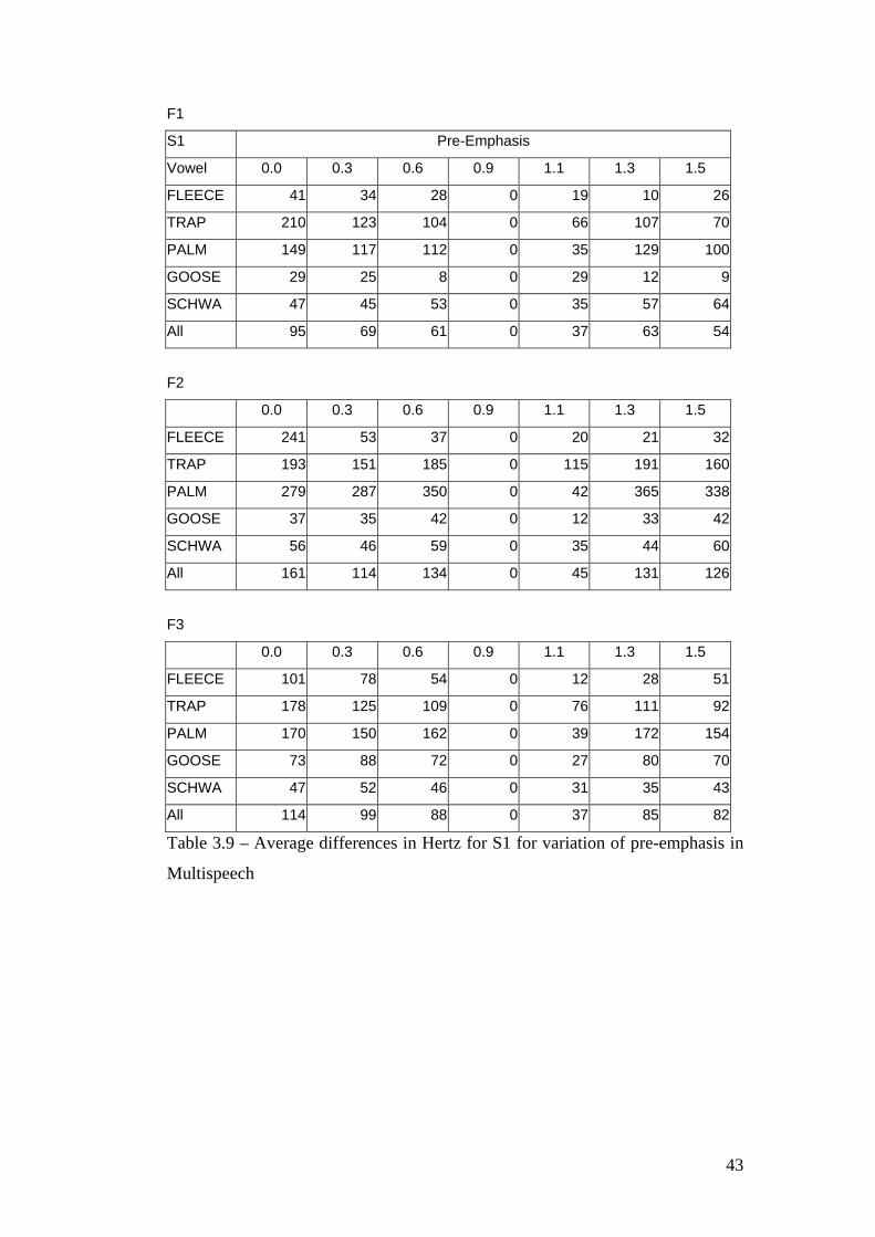
F1 S1 Pre-Emphasis

Vowel 0.0 0.3 0.6 0.9 1.1 1.3 1.5

FLEECE 41 34 28 0 19 10 26

TRAP 210 123 104 0 66 107 70

PALM 149 117 112 0 35 129 100

GOOSE 29 25 8 0 29 12 9

SCHWA 47 45 53 0 35 57 64

All 95 69 61 0 37 63 54

F2 0.0 0.3 0.6 0.9 1.1 1.3 1.5

FLEECE 241 53 37 0 20 21 32

TRAP 193 151 185 0 115 191 160

PALM 279 287 350 0 42 365 338

GOOSE 37 35 42 0 12 33 42

SCHWA 56 46 59 0 35 44 60

All 161 114 134 0 45 131 126

F3 0.0 0.3 0.6 0.9 1.1 1.3 1.5

FLEECE 101 78 54 0 12 28 51

TRAP 178 125 109 0 76 111 92

PALM 170 150 162 0 39 172 154

GOOSE 73 88 72 0 27 80 70

SCHWA 47 52 46 0 31 35 43

All 114 99 88 0 37 85 82

Table 3.9 – Average differences in Hertz for S1 for variation of pre-emphasis in

Multispeech

43

F1 S2 Pre-Emphasis

Vowel 0.0 0.3 0.6 0.9 1.1 1.3 1.5

FLEECE 18 13 11 0 2 6 9

TRAP 156 92 68 0 22 47 72

PALM 38 32 20 0 2 24 26

GOOSE 12 10 7 0 2 9 8

SCHWA 17 10 8 0 3 12 15

All 48 31 23 0 6 20 26

F2 0.0 0.3 0.6 0.9 1.1 1.3 1.5

FLEECE 185 39 8 0 0 2 6

TRAP 132 95 77 0 22 46 74

PALM 146 139 104 0 20 109 130

GOOSE 125 200 184 0 21 109 169

SCHWA 43 25 19 0 1 23 27

All 126 99 78 0 13 58 81

F3 0.0 0.3 0.6 0.9 1.1 1.3 1.5

FLEECE 184 283 156 0 15 32 122

TRAP 178 123 68 0 25 45 55

PALM 150 126 86 0 22 87 115

GOOSE 163 187 152 0 16 109 154

SCHWA 81 54 26 0 0 26 3

All 151 154 98 0 16 60 90

Table 3.10 – Average differences in Hertz for S2 for variation of pre-emphasis in

Multispeech

The pre-emphasis parameter in Multispeech specifies the amount of pre-

emphasis applied to the speech whereas the parameter in Praat specifies from

which frequency the pre-emphasis is applied. Since the parameters are not

equivalent, the results from the two pieces of software should not be directly

compared. However, one observation which can be made is that the differences

seen in the results for Multispeech are greater than those for Praat.

44

The results show that the differences are roughly equivalent either side of the

default setting with slightly larger differences at the lower pre-emphasis settings.

The overall differences are less for F1 than for F2 and F3. A comparison across

the vowel categories shows that for S1, the TRAP and PALM categories are

affected most by the variation of the pre-emphasis parameter, whilst for S2 the

TRAP category for F1 has relatively larger difference values in comparison with

the other vowel categories.

The F2 values for GOOSE in S2’s results show the greatest difference from the

default reference values, whilst for S1, the F2 values for GOOSE show the

smallest difference.

In the case of the results for the LPC variation a clear pattern emerged that the

LPC settings lower than the default setting produced formant measurements

which were above those in the reference set and for LPC settings higher than the

default the formant values were lower than the reference set. Examining the raw

formant measurements for the pre-emphasis variations showed no such pattern.

The results appear to be randomly distributed both above and below the reference

values regardless of the pre-emphasis setting. This is true for both speakers.

3.2.2.7 Wavesurfer Pre-Emphasis Variation

Table 3.11 below shows the difference results for the pre-emphasis variation in

Wavesurfer for S1, while table 3.12 shows the results for S2.

F1 S1 Pre-Emphasis

Vowel 0.0 0.1 0.3 0.5 0.7 0.9

FLEECE 13 12 10 6 0 14

TRAP 252 221 195 124 0 261

PALM 322 303 265 277 0 318

GOOSE 24 23 19 9 0 21

SCHWA 32 32 29 20 0 32

All 128 118 104 87 0 129

45

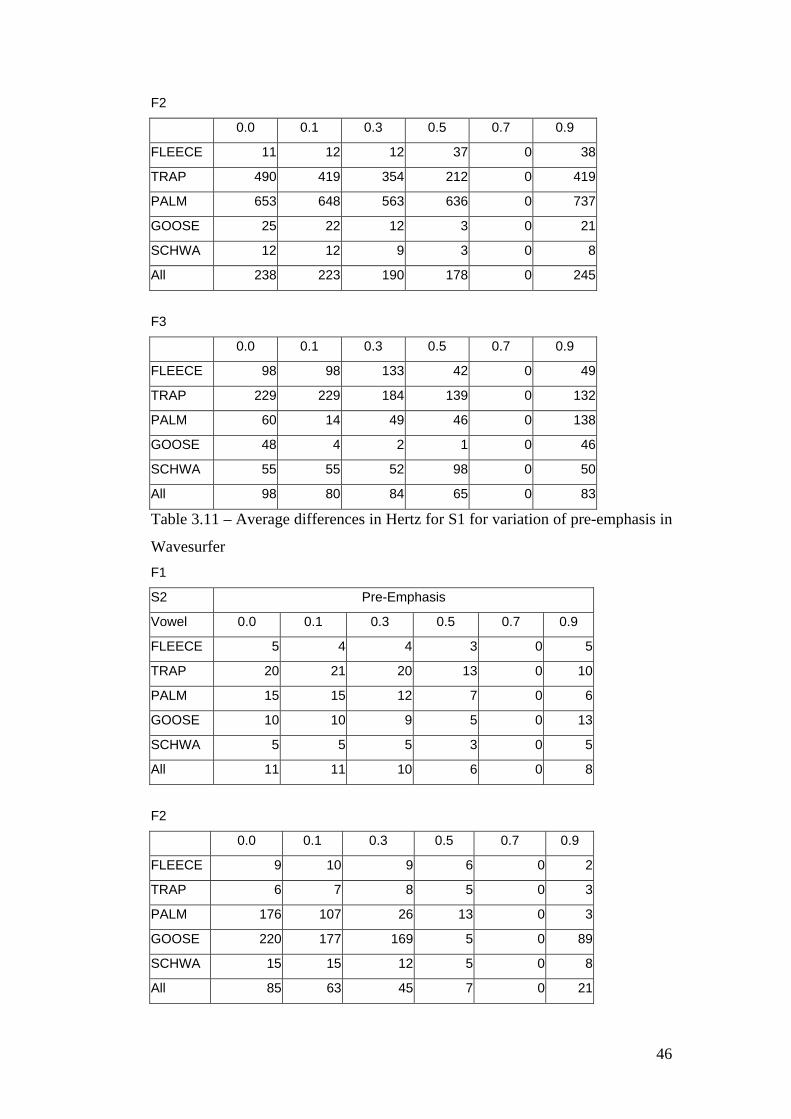
F2 0.0 0.1 0.3 0.5 0.7 0.9

FLEECE 11 12 12 37 0 38

TRAP 490 419 354 212 0 419

PALM 653 648 563 636 0 737

GOOSE 25 22 12 3 0 21

SCHWA 12 12 9 3 0 8

All 238 223 190 178 0 245

F3 0.0 0.1 0.3 0.5 0.7 0.9

FLEECE 98 98 133 42 0 49

TRAP 229 229 184 139 0 132

PALM 60 14 49 46 0 138

GOOSE 48 4 2 1 0 46

SCHWA 55 55 52 98 0 50

All 98 80 84 65 0 83

Table 3.11 – Average differences in Hertz for S1 for variation of pre-emphasis in

Wavesurfer F1 S2 Pre-Emphasis

Vowel 0.0 0.1 0.3 0.5 0.7 0.9

FLEECE 5 4 4 3 0 5

TRAP 20 21 20 13 0 10

PALM 15 15 12 7 0 6

GOOSE 10 10 9 5 0 13

SCHWA 5 5 5 3 0 5

All 11 11 10 6 0 8

F2 0.0 0.1 0.3 0.5 0.7 0.9

FLEECE 9 10 9 6 0 2

TRAP 6 7 8 5 0 3

PALM 176 107 26 13 0 3

GOOSE 220 177 169 5 0 89

SCHWA 15 15 12 5 0 8

All 85 63 45 7 0 21

46

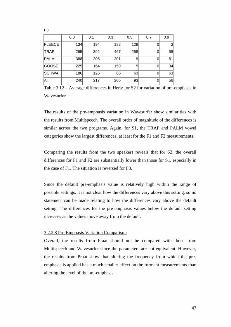
F3 0.0 0.1 0.3 0.5 0.7 0.9

FLEECE 134 194 133 128 0 3

TRAP 265 392 467 258 0 59

PALM 388 206 201 9 0 61

GOOSE 225 164 159 5 0 94

SCHWA 186 126 66 63 0 63

All 240 217 205 93 0 56

Table 3.12 – Average differences in Hertz for S2 for variation of pre-emphasis in

Wavesurfer

The results of the pre-emphasis variation in Wavesurfer show similarities with

the results from Multispeech. The overall order of magnitude of the differences is

similar across the two programs. Again, for S1, the TRAP and PALM vowel

categories show the largest differences, at least for the F1 and F2 measurements.

Comparing the results from the two speakers reveals that for S2, the overall

differences for F1 and F2 are substantially lower than those for S1, especially in

the case of F1. The situation is reversed for F3.

Since the default pre-emphasis value is relatively high within the range of

possible settings, it is not clear how the differences vary above this setting, so no

statement can be made relating to how the differences vary above the default

setting. The differences for the pre-emphasis values below the default setting

increases as the values move away from the default.

3.2.2.8 Pre-Emphasis Variation Comparison

Overall, the results from Praat should not be compared with those from

Multispeech and Wavesurfer since the parameters are not equivalent. However,

the results from Praat show that altering the frequency from which the pre-

emphasis is applied has a much smaller effect on the formant measurements than

altering the level of the pre-emphasis.

47

The results from Multispeech and Wavesurfer show a comparable level of

variation across the different analysis settings and again differences are seen

across the results obtained for the different vowel categories. Differences are also

present between the two speakers. The overall levels of variation encountered are

substantially lower than those found for the LPC variation results.

3.2.2.9 Praat Frame Width Variation

Table 3.13 below shows the difference results for the frame width variation in

Praat for S1, while table 3.14 shows the results for S2. F1 S1 Frame Width (s)

Vowel 0.005 0.010 0.015 0.020 0.025 0.030 0.035 0.040 0.045 0.050

FLEECE 25.6 5.3 2.3 0.8 0.0 0.3 0.5 0.5 0.6 0.6

TRAP 68.7 22.4 9.5 2.7 0.0 1.3 2.0 2.4 2.7 3.0

PALM 88.5 25.2 8.4 2.8 0.0 1.2 1.7 2.0 2.1 2.2

GOOSE 66.5 5.4 2.4 1.0 0.0 0.4 0.7 0.7 0.6 0.8

SCHWA 22.4 5.6 1.9 0.7 0.0 0.3 0.5 0.6 0.6 0.6

All 54.3 12.8 4.9 1.6 0.0 0.7 1.1 1.2 1.3 1.4

F2 0.005 0.010 0.015 0.020 0.025 0.030 0.035 0.040 0.045 0.050

FLEECE 43.7 17.7 5.9 2.5 0.0 1.8 3.0 3.2 3.7 3.8

TRAP 54.1 7.8 2.5 0.9 0.0 0.4 0.5 0.6 0.7 0.8

PALM 67.7 13.9 2.7 0.8 0.0 0.4 0.6 0.7 0.8 0.9

GOOSE 28.8 10.9 4.4 1.4 0.0 0.8 1.2 1.5 1.7 1.9

SCHWA 29.9 6.7 3.2 1.1 0.0 0.5 0.7 0.9 1.0 1.2

All 44.8 11.4 3.7 1.3 0.0 0.8 1.2 1.4 1.6 1.7

F3 0.005 0.010 0.015 0.020 0.025 0.030 0.035 0.040 0.045 0.050

FLEECE 51.2 18.3 8.8 4.9 0.0 4.4 6.8 7.5 11.3 11.5

TRAP 38.5 20.8 10.0 3.2 0.0 1.2 1.7 1.8 1.9 1.9

PALM 52.0 18.7 6.3 2.2 0.0 1.1 1.7 2.0 2.3 2.5

GOOSE 83.9 15.4 8.0 3.4 0.0 1.8 3.3 4.1 3.9 4.7

SCHWA 38.9 8.4 3.8 1.3 0.0 0.6 0.8 0.9 1.1 1.1

All 52.9 16.3 7.4 3.0 0.0 1.8 2.8 3.3 4.1 4.4

Table 3.13 – Average differences in Hertz for S1 for variation of frame width in

Praat

48

F1 S2 Frame Width (s)

Vowel 0.005 0.010 0.015 0.020 0.025 0.030 0.035 0.040 0.045 0.050

FLEECE 17.2 3.7 1.1 0.3 0.0 0.2 0.3 0.3 0.4 0.4

TRAP 27.0 7.3 2.0 0.6 0.0 0.3 0.5 0.7 0.8 0.9

PALM 45.0 9.2 2.5 0.7 0.0 0.3 0.6 0.7 0.8 0.8

GOOSE 19.9 4.3 1.1 0.8 0.0 1.8 1.6 1.6 3.3 0.8

SCHWA 9.5 4.0 1.3 0.4 0.0 0.2 0.3 0.4 0.4 0.5

All 23.7 5.7 1.6 0.5 0.0 0.6 0.6 0.7 1.1 0.7

F2 0.005 0.010 0.015 0.020 0.025 0.030 0.035 0.040 0.045 0.050

FLEECE 38.3 6.8 1.9 0.9 0.0 0.6 1.1 1.8 2.4 3.2

TRAP 22.4 7.8 3.0 1.0 0.0 0.5 0.8 1.0 1.2 1.3

PALM 30.1 16.5 4.6 1.4 0.0 0.7 1.3 1.7 2.0 2.4

GOOSE 228.5 60.0 28.8 24.4 0.0 15.4 6.8 8.6 11.5 30.6

SCHWA 21.7 7.0 2.6 0.8 0.0 0.3 0.5 0.6 0.7 0.7

All 68.2 19.6 8.2 5.7 0.0 3.5 2.1 2.8 3.6 7.7

F3 0.005 0.010 0.015 0.020 0.025 0.030 0.035 0.040 0.045 0.050

FLEECE 123.2 43.2 11.9 4.7 0.0 3.5 6.2 8.0 9.2 10.1

TRAP 30.3 4.6 1.5 0.5 0.0 0.4 0.7 1.1 1.3 1.5

PALM 25.2 7.5 2.6 0.8 0.0 0.6 1.1 1.4 1.6 1.7

GOOSE 170.9 45.6 17.9 17.0 0.0 6.0 2.1 2.7 3.4 14.1

SCHWA 29.5 6.7 3.0 1.1 0.0 0.6 0.8 1.0 1.1 1.1

All 75.9 21.5 7.4 4.8 0.0 2.2 2.2 2.8 3.3 5.7

Table 3.14 – Average differences in Hertz for S2 for variation of frame width in

Praat

Tables 3.13 and 3.14 above show that the variation caused by altering the frame

width follows the now familiar pattern of the differences increasing as the

analysis setting moves away from the default. However, the differences present

for settings above the default frame width setting are considerably lower than

those found with a frame width less than the default. The variation in differences

is reasonably consistent across all vowel categories and the three formants,

49

except for the GOOSE category for S2 for F2 and F3 where the differences are

relatively larger. On the whole, the differences values are small.

3.2.2.10 Multispeech Frame Width Variation

Table 3.15 below shows the difference results for the frame width variation in

Multispeech for S1, while table 3.16 shows the results for S2.

F1 S1 Frame Width (s)

Vowel 0.005 0.010 0.015 0.020 0.025 0.030

FLEECE 76 0 30 28 28 29

TRAP 112 0 188 189 151 128

PALM 132 0 111 125 106 130

GOOSE 88 0 13 16 15 15

SCHWA 158 0 30 45 38 39

All 113 0 74 81 68 68

F2 0.005 0.010 0.015 0.020 0.025 0.030

FLEECE 71 0 32 33 37 35

TRAP 215 0 379 395 312 259

PALM 457 0 412 427 309 463

GOOSE 122 0 46 76 48 50

SCHWA 194 0 46 70 64 62

All 212 0 183 200 154 174

F3 0.005 0.010 0.015 0.020 0.025 0.030

FLEECE 92 0 54 57 59 54

TRAP 138 0 219 220 194 136

PALM 273 0 224 257 239 266

GOOSE 412 0 115 173 208 166

SCHWA 231 0 45 69 62 65

All 229 0 131 155 152 137

Table 3.15 – Average differences in Hertz for S1 for variation of frame width in

Multispeech

50

F1 S2 Frame Width (s)

Vowel 0.005 0.010 0.015 0.020 0.025 0.030

FLEECE 64 0 15 18 20 23

TRAP 128 0 68 73 69 70

PALM 27 0 9 9 10 10

GOOSE 82 0 10 11 13 14

SCHWA 65 0 8 11 10 10

All 73 0 22 24 24 25

F2 0.005 0.010 0.015 0.020 0.025 0.030

FLEECE 52 0 15 18 22 24

TRAP 145 0 88 99 98 98

PALM 187 0 105 150 139 100

GOOSE 314 0 179 241 308 272

SCHWA 179 0 22 24 25 24

All 175 0 82 107 118 103

F3 0.005 0.010 0.015 0.020 0.025 0.030

FLEECE 169 0 93 72 134 166

TRAP 266 0 110 110 114 112

PALM 143 0 66 115 97 88

GOOSE 270 0 144 179 254 224

SCHWA 193 0 65 67 73 46

All 208 0 96 109 134 127

Table 3.16 – Average differences in Hertz for S2 for variation of frame width in

Multispeech

In the case of S1 the results for altering frame width in Multispeech are slightly

different from the normal pattern found for the variation of the other analysis

parameters. Again, the differences vary as the frame width moves away from the

default values, however, the greatest differences generally occur at the 0.02

second setting rather than the highest setting of 0.03 seconds (ignoring the setting

below the default). There is also a marked difference between vowel categories.

For F1 and F2 the differences for TRAP and PALM are generally several orders

51

of magnitude greater than for the other categories. In the case of F3, the greatest

differences occur for TRAP, PALM and GOOSE. The results for F2 also show

variation between the vowel categories. For F1, the results for TRAP are greater

than those in the other categories. For F2, TRAP, PALM and GOOSE have

larger difference values than for FLEECE and SCHWA.

Comparing the results for the two speakers shows that S2 generally has smaller

difference values that S1. This is most noticeable in the case of F1.

Overall, the difference values are generally greater than those seen for Praat,

even though the range of frame width values is actually smaller for Multispeech.

3.2.2.11 Wavesurfer Frame Width Variation

Table 3.17 below shows the difference results for the frame width variation in

Wavesurfer for S1, while table 3.18 shows the results for S2.

F1 S1 Frame Width (s)

Vowel 0.01 0.02 0.03 0.04 0.049 0.06 0.07 0.08 0.09 0.10

FLEECE 56 15 7 3 0 3 4 4 4 4

TRAP 239 152 14 44 0 5 83 148 189 153

PALM 169 115 42 4 0 79 146 189 235 235

GOOSE 32 12 8 3 0 2 2 2 2 3

SCHWA 96 21 10 6 0 3 5 7 8 9

All 118 63 16 12 0 18 48 70 88 81

F2 0.01 0.02 0.03 0.04 0.049 0.06 0.07 0.08 0.09 0.10

FLEECE 60 13 7 5 0 6 7 7 8 8

TRAP 520 289 7 73 0 3 216 353 348 283

PALM 456 277 96 8 0 160 323 407 491 491

GOOSE 30 43 7 9 0 9 8 9 8 8

SCHWA 229 11 3 3 0 2 3 3 4 4

All 259 126 24 20 0 36 111 156 172 159

52

F3 0.01 0.02 0.03 0.04 0.049 0.06 0.07 0.08 0.09 0.10

FLEECE 212 34 58 16 0 48 12 22 22 21

TRAP 292 152 52 46 0 3 46 129 176 132

PALM 311 85 116 58 0 3 6 10 55 55

GOOSE 79 12 8 5 0 7 5 5 5 5

SCHWA 345 132 151 105 0 139 86 140 141 142

All 248 83 77 46 0 40 31 61 80 71

Table 3.17 – Average differences in Hertz for S1 for variation of frame width in

Wavesurfer F1 S2 Frame Width (s)

Vowel 0.01 0.02 0.03 0.04 0.049 0.06 0.07 0.08 0.09 0.10

FLEECE 65 19 6 2 0 1 2 2 3 3

TRAP 119 98 3 3 0 2 6 6 6 5

PALM 128 9 3 2 0 1 2 2 2 3

GOOSE 144 10 5 1 0 1 1 2 2 2

SCHWA 238 7 2 1 0 1 1 2 2 2

All 139 29 4 2 0 1 2 3 3 3

F2 0.01 0.02 0.03 0.04 0.049 0.06 0.07 0.08 0.09 0.10

FLEECE 43 8 5 2 0 1 3 4 5 7

TRAP 230 114 2 3 0 2 3 3 4 4

PALM 613 237 230 154 0 3 4 4 4 5

GOOSE 181 80 5 69 0 2 3 84 84 85

SCHWA 272 4 3 1 0 1 2 2 3 3

All 268 88 49 46 0 2 3 20 20 21

F3 0.01 0.02 0.03 0.04 0.049 0.06 0.07 0.08 0.09 0.10

FLEECE 331 218 92 57 0 57 57 142 143 144

TRAP 541 275 61 67 0 3 5 5 5 60

PALM 627 278 204 207 0 3 4 5 6 7

GOOSE 404 74 18 123 0 39 41 94 95 96

SCHWA 342 5 65 2 0 1 3 3 4 4

All 449 170 88 91 0 21 22 50 51 62

Table 3.18 – Average differences in Hertz for S2 for variation of frame width in

Wavesurfer

53

Again, the same pattern is seen in the results where the difference increases as

the frame width setting moves away from the default. The differences seen are

generally greater when the frame width is less than the default setting. For S1, a

feature of the results common with those for S1 in Multispeech is that overall,

the greatest difference above the default value is not found at the highest setting

(0.10 seconds), but at a lower setting (0.09 seconds). It is not clear why this

should be the case for either software. Another similarity with the results from

Multispeech is that for F1 and F2, the TRAP and PALM tokens show a much

higher level of difference from the default value than the other vowel categories

do. However, unlike Multispeech, in the case of F3, a large difference is also

found for SCHWA. The F3 differences for PALM above the default setting are

also much less than those seen for F1 and F2.

The results for S2 show some interesting features. For F1, the difference values

above the default setting are very small, with the average across the vowel

categories being no more than 3 Hz. The difference values for the GOOSE

category for F2 show an odd variation. As the frame width decreases from the

default the difference equals 69 Hz, then 5 Hz and then jumps up to 80 Hz. As

the frame width increases from the default the difference equals 2 Hz, then 3 Hz

and then jumps up to 84 Hz. These strange results are most likely caused by the

misidentification of formants which occurs within this category.

3.2.2.12 Frame Width Variation Comparison

An overall comparison of the three systems reveals that the smallest amount of

variation is present in the results for Praat. This is followed second by

Wavesurfer. Even though the range of the frame widths is less in Multispeech

than the other two programs, it exhibits the greatest amount of variation. Again,

patterns of difference are seen across the vowel categories, some of which are

present across the different programs.

3.2.3 Statistical Analysis

The results above show clearly that altering the analysis settings does alter the

measured formant values and the variation produced is different for the different

54

programs being compared. In order to find out if the variation seen can be

considered as significant, it is necessary to carry out a statistical analysis. As

described above in section 3.1 the paired t-test was chosen as the test of

significance. Two significance levels were chosen, 0.01 and 0.05. The 0.01

significance level is a more stringent test which requires a lower t-test result to

provide support for the experimental hypothesis that variation is occurring

between the measured formant values and the reference values.

The paired t-tests were carried out between the reference results and the

measurements from each program for all of the analysis settings for both

speakers. The comparisons were carried out separately for each vowel category.

This gave 15 t-test results per analysis setting since 5 vowel categories were

analysed for all three formants. In order to condense the results, the number of

tests which returned a result lower than the significance levels of 0.01 and 0.05

have been summed for each analysis setting. The results are displayed in table

3.19 below.

LPC Variation

Praat

LPC Order 6 8 10 12 14 16 18

P<0.05 14 15 N/A 10 11 11 14 S1

P<0.01 14 13 N/A 6 10 10 13

P<0.05 14 13 N/A 9 10 13 15 S2

P<0.01 14 12 N/A 7 8 12 15

Multispeech

LPC Order 6 8 10 12 14 16 18

P<0.05 14 12 7 N/A 9 12 13 S1

P<0.01 14 11 5 N/A 5 12 13

P<0.05 13 10 8 N/A 5 13 15 S2

P<0.01 8 10 7 N/A 4 13 15

55

Wavesurfer

LPC Order 10 11 12 13 14 15 16 17 18

P<0.05 11 7 N/A 8 10 9 10 10 11S1

P<0.01 7 7 N/A 7 9 6 9 8 9

P<0.05 10 10 N/A 5 6 4 5 6 7S2

P<0.01 8 7 N/A 2 4 3 3 5 5

Pre-Emphasis Variation

Praat

Pre-Emphasis (Hz) 1 25 50 75 100 125 150

P<0.05 13 13 N/A 13 13 13 13 S1

P<0.01 13 13 N/A 13 13 13 13

P<0.05 13 13 N/A 13 13 13 12 S2

P<0.01 13 13 N/A 13 13 13 11

Multispeech

Pre-Emphasis 0.0 0.3 0.6 0.9 1.1 1.3 1.5

P<0.05 4 2 5 N/A 0 9 5 S1

P<0.01 2 1 4 N/A 0 7 4

P<0.05 7 4 9 N/A 0 5 6 S2

P<0.01 3 2 3 N/A 0 2 2

Wavesurfer

Pre-Emphasis 0.0 0.1 0.3 0.5 0.7 0.9

P<0.05 5 5 6 4 N/A 9 S1

P<0.01 4 4 5 4 N/A 8

P<0.05 8 7 9 8 N/A 6 S2

P<0.01 4 6 8 7 N/A 5

Frame Width Variation

Praat

Frame Width (s) 0.005 0.010 0.015 0.020 0.025 0.030 0.035 0.040 0.045 0.050

P<0.05 7 2 1 0 N/A 2 4 3 5 4 S1

P<0.01 4 0 0 0 N/A 0 0 0 0 0

P<0.05 7 7 5 4 N/A 3 6 6 5 4 S2

P<0.01 5 3 3 2 N/A 2 3 3 3 3

56

Multispeech

Frame Width (s) 0.005 0.010 0.015 0.020 0.025 0.30

P<0.05 7 N/A 7 4 6 8S1

P<0.01 4 N/A 2 0 3 3

P<0.05 10 N/A 7 8 8 9S2

P<0.01 6 N/A 6 8 8 6

Wavesurfer

Frame Width (s) 0.01 0.02 0.03 0.04 0.049 0.06 0.07 0.08 0.09 0.1

P<0.05 5 2 1 1 N/A 2 2 3 4 4 S1

P<0.01 3 1 1 0 N/A 0 0 0 1 1

P<0.05 12 5 4 2 N/A 2 2 2 2 3 S2

P<0.01 6 4 2 1 N/A 2 1 1 2 2

Table 3.19 – Condensed results of paired t-tests for S1 and S2

In the table above, the number of significant results are measured out of a

possible total of 15. A high value near 15 indicates that the analysis setting

produces variation for most vowel categories across all three formants. A low

value indicates that the analysis setting produces little variation across the vowel

categories and formants.

The results of the statistical tests generally confirm the pattern that was seen in

the difference results discussed above, which is that the amount of variation in

the formant measurements decreases as the analysis setting approaches the

default value. This pattern is clearest for the LPC variation results.

The results of the statistical tests for the LPC order variation show that a

relatively high degree of variation occurs across all of the LPC order settings.

The least amount of variation occurs for S2 in Wavesurfer. Considering the

results from both speakers, Praat shows the highest degree of variation, whilst

Wavesurfer shows the least. This is in agreement with impression gained from

examining the difference measurements.

57

The interpretation of the results of the statistical tests becomes less

straightforward when considering the results for the pre-emphasis variation. The

results for Praat show that all of the tests except for 2 resulted in a combined

score of 13. This indicates that there is a high degree of variation occurring in the

formant measurements. Examining the difference results for pre-emphasis

variation in Praat shown in table 3.7 and table 3.8 reveals that the difference

between the analysis settings and the default settings was generally small and in

some instances less than 1. The natural assumption would be that this group of

analysis settings would produce statistical results that showed a very low level of

variation (i.e. a low number in table 3.19 above). However, this is not the case.

The reason for this is that there is very little overlap between the default

reference values and those generated with the different pre-emphasis settings.

Because of this the statistical tests see the data as being different even though the

absolute difference between the results is very small. The test results therefore

support the experimental hypothesis that variation is occurring.

The test results for the pre-emphasis variation in Multispeech and Wavesurfer

show that approximately half of the formant measurements across the vowel

categories produce results which can be considered as showing no variation. The

results for Multispeech show that the pre-emphasis setting of 1.1 produced no

significant results for any vowel for any formant. This indicates that there is no

significant variation between the results produced with a setting of 0.9 and 1.1.

The results for the frame width analysis for all three pieces of software show a

very strong support of the null hypothesis across all three formants for each of

the vowel categories. For S1, when the significance level is 0.01, all analysis

settings bar one indicate that there is no significant difference between the

reference values and the measured values. Examining the raw data and the

difference values for Praat shows that the level of variation in the results is

relatively small and the t-test results do reflect what is apparent in the data.

3.3 Discussion

Having conducted an analysis of the results, I had hoped to be able to draw up a

set of recommendations or guidelines which could be used by forensic

58

phoneticians when carrying out formant analyses. Unfortunately this has not

been possible due to the complex nature of the results and a lack of obvious

patterning beyond the general observations made in the results section above.

The kind of recommendations I had envisaged setting out would have included,

for example, threshold levels for the analysis settings above and below which the

level of variation was significantly large.

However, some general recommendations can be made on the basis of the results

obtained. The first recommendation is that all formant measurements generated

by formant trackers should be compared with a spectrogram. Although this study

has not been concerned with the accuracy of formant measurements, it is clear

that errors must be occurring in some of the measurements. This is illustrated

below in figures 3.4 to 3.6 which show the average reference formant

measurements generated from the default settings for each of the three programs

for S1.

0

200

400

600

800

1000

1200

FLEECE TRAP PALM GOOSE SCHWA

F1 F

requ

ency

(Hz)

PraatMultispeechWavesurfer

Figure 3.4 - F1 values with default settings for all three programs for S1

59

0

500

1000

1500

2000

2500

FLEECE TRAP PALM GOOSE SCHWA

F2 F

requ

ency

(Hz)

PraatMultispeechWavesurfer

Figure 3.5 - F2 values with default settings for all three programs for S1

0

500

1000

1500

2000

2500

3000

3500

4000

FLEECE TRAP PALM GOOSE SCHWA

F3 F

requ

ency

(Hz)

PraatMultispeechWavesurfer

Figure 3.6 - F3 values with default settings for all three programs for S1

60

The differences between the results for the three programs are, for some vowel

categories, very large. The greatest differences occur for the F3 values and in the

case of the vowel category PALM the difference between the results for Praat

and Wavesurfer is 858 Hz and for GOOSE the difference is 983 Hz. These

significantly large differences are most probably caused by the misidentification

of formants which occurred in the results of Wavesurfer for both S1 and S2. The

differences present between the default results for Praat and Multispeech are also

relatively large, especially for the F2 values for the TRAP and PALM categories

where the difference is of the order of 473 Hz and 540 Hz respectively.

Accepting on trust that the default settings will produce accurate and reliable

results is a very dangerous assumption.

The second recommendation is that if a series of vowels from different categories

are being measured with different LPC orders, a consistent setting should be used

for each category. This does not mean that the same LPC order should be used

for all categories. For example, consider a series of tokens containing words with

the TRAP vowel and the formants are being measured with an LPC order of 10.

If the next word in the series has a different category vowel it may be necessary

to change the LPC order to 12 for example. If the following token contains

another TRAP vowel and the LPC order is not changed back to 10, a different

value will be measured to the one that would have been recorded if the LPC had

been returned to 10. This kind of inconsistency in LPC setting will potentially

skew the resulting formant measurements.

Another potential outcome of the study could have been a recommendation for

which software produced the most stable results and showed the least variation.

Having studied the results from each of the three software systems it is not clear

which system produces the least variation overall. I would, however, attach a

particular note of caution to Wavesurfer which showed a tendency towards the

misidentification of formants. It is not clear what the cause of this was. It could

be the two speakers chosen have particular types of voice which Wavesurfer

cannot cope with, or it could be a more significant problem. Although, ignoring

the results which are affected by misidentification, the variation present in

Wavesurfer results in relatively small differences.

61

4 - Conclusions

The overall findings of the study are that the choice of analysis settings does

have an effect on the resulting formant measurements. The overall pattern seen in

the results is that as an analysis setting is increased or decreased away from the

default value, the difference increases between the resulting formant

measurement and the default reference measurement.

The overall degree of variation is different for each of the analysis parameters.

The largest variation occurs when the LPC order is varied. It is difficult to make

an overall judgement between the pre-emphasis and the frame width settings as

to which produces the least variation.

The consequence of the study for forensic phoneticians is that they should be

aware of the differences that altering analysis settings can have on formant

measurements.

4.1 Improvements and Further Work

The study carried out was only concerned with the variation present in the

formant measurements and not with the accuracy of the measurements in

absolute terms. It would be worthwhile to continue this work and to make an

assessment of the accuracy of the formant measurements.

An initial examination of the formant values obtained from the telephone

recordings showed some interesting differences from the microphone recordings,

such as an absence of misidentified formants in the results from Wavesurfer.

This study has only considered speech from two people. The results have shown

that the performance of the software is different for the two speakers. It may be

the case that the performance of the software is dependent on a feature of the

voice which is not adequately represented by only two speakers. Extending the

study to include more speakers could throw light on this.

62

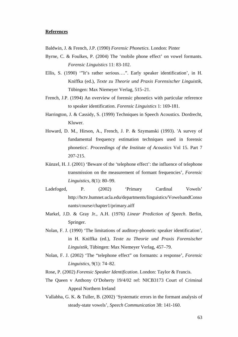
References

Baldwin, J. & French, J.P. (1990) Forensic Phonetics. London: Pinter

Byrne, C. & Foulkes, P. (2004) The ‘mobile phone effect’ on vowel formants.

Forensic Linguistics 11: 83-102.

Ellis, S. (1990) ‘”It’s rather serious….”. Early speaker identification’, in H.

Kniffka (ed.), Texte zu Theorie und Praxis Forensischer Linguistik,

Tübingen: Max Niemeyer Verlag, 515–21.

French, J.P. (1994) An overview of forensic phonetics with particular reference

to speaker identification. Forensic Linguistics 1: 169-181.

Harrington, J. & Cassidy, S. (1999) Techniques in Speech Acoustics. Dordrecht,

Kluwer.

Howard, D. M., Hirson, A., French, J. P. & Szymanski (1993). 'A survey of

fundamental frequency estimation techniques used in forensic

phonetics'. Proceedings of the Institute of Acoustics Vol 15. Part 7

207-215.

Künzel, H. J. (2001) ‘Beware of the ‘telephone effect’: the influence of telephone

transmission on the measurement of formant frequencies’, Forensic

Linguistics, 8(1): 80–99.

Ladefoged, P. (2002) ‘Primary Cardinal Vowels’

http://hctv.humnet.ucla.edu/departments/linguistics/VowelsandConso

nants/course/chapter1/primary.aiff

Markel, J.D. & Gray Jr., A.H. (1976) Linear Prediction of Speech. Berlin,

Springer.

Nolan, F. J. (1990) ‘The limitations of auditory-phonetic speaker identification’,

in H. Kniffka (ed.), Texte zu Theorie und Praxis Forensischer

Linguistik, Tübingen: Max Niemeyer Verlag, 457–79.

Nolan, F. J. (2002) ‘The “telephone effect” on formants: a response’, Forensic

Linguistics, 9(1): 74–82.

Rose, P. (2002) Forensic Speaker Identification. London: Taylor & Francis.

The Queen v Anthony O’Doherty 19/4/02 ref: NICB3173 Court of Criminal

Appeal Northern Ireland

Vallabha, G. K. & Tuller, B. (2002) ‘Systematic errors in the formant analysis of

steady-state vowels’, Speech Communication 38: 141-160.

63

Wells, J. C. (1982) Accents of English (3 vols.), Cambridge: Cambridge

University Press.

64