VAR Models Jesus Gonzalo - UC3Mjgonzalo/teaching/PhdTimeSeries/VAR models 2017.pdfVAR Models Jesus...

VAR Models

Jesus Gonzalo

Universidad Carlos III de Madrid

Time Series Econometrics

Jesus Gonzalo VAR Models Time Series 1 / 1

Some References

Hamilton, J., Time Series Analysis. Princeton University Press, 1994.

Canova, F.,Methods for Applied Macroeconomic Research. Princeton,2007.

Lutkepohl, H., New Inroduction to Multiple Time Series Analysis,second edition. Springer Verlag, 2007.

Watson, M., VAR and Cointegration in Handbook of Econometrics,1994.

Stock, J., and M. Watson, Lecture Notes on What is New inEconometrics at NBER, 2008.


Goals of VAR models

Let YtK×1

be a vector of macro time series, and let εrt denote an

unanticipated (surprise, shock. . . ) monetary policy intervention. Wewant to know the DYNAMIC CAUSAL EFFECT of εrt on Yt :

(∗) ∂Yt+h

∂εrt, h = 1, 2, 3, . . . IRF (1)

given all the other possible interventions constant.

Exercise: Calculate the IRF for a univariable AR(1) model:Yt = φYt−1 + εt , |φ| ≤ 1

The challenge is to estimate ∂Yt+h

∂εrt from observational data.

(**) Granger causality: Does Y2t , ...,Ykt Granger cause Y1t?

(***) Do not forget prediction.


Wold Decomposition

Everything starts from the Wold decomposition for YtK×1

(weak

stationary):

YtK×1

= C (L)(K×K )

et(K×1)

; C (0) = I ; Σe unrestricted

with et a vector white noise E (et) = 0, E (etet−j ) = 0, j 6= 0Remark: Review univariate Wold DecompositionExercise: Following the same “reasoning” of the univariate WoldDecomposition, obtain et and C (L).C (L) gives us the response of Yt to unit impulses to each of theelements of et .We could calculate instead the responses of Yt to new shocks thatare linear combinations of the old shocks:

ε2×1

= Q(2×2)

et(2×1)

=

[1 0

0.5 1

] [e1t

e2t

]=

[e1t

0.5e1t + e2t

]The MA representation can be written as: Yt = C (L)Q−1Qet = D(L)εt


Wold Decomposition

Question: Which linear combination of shocks should we look at?Answer: It seems that the most interesting are the linearcombinations that produce orthogonal shocks: Σε = DiagonalOrthogonal shocks ≡ Structural shocksWe are going to pick a Q matrix s.t E (εtε′t) = I . To do that choosea Q s.t.

Q−1(Q−1)′ = Σe

ThenE (εtε

′t) = E (Qete

′tQ′) = QΣeQ

′ = I

One way to construct such a Q is via Choleski decomposition: “TheCholeski decomposition of a Hermitian p.d matrix A is adecomposition of the form:

A = LL∗

where L is a lower triangular matrix with real and positive diagonalentries and L∗ is the conjugate transpose.”


Wold Decomposition

Unfortunately there are many different Q ′s that act as “square root”matrices for Σ−1

e . Given a Q we can form another Q∗ = RQ with Ran orthogonal matrix:

RR ′ = I , Q∗ΣeQ∗′ = RQΣeQ

′R ′ = RR ′ = I

Example: Square roots of [1 00 1

]:

1

t

[∓s ∓r∓r ±s

];

1

t

[±s ∓r∓r ∓s

]; ...;

[1 00 ±1

]and

[±1 00 1

]where (r , s, t) is any set of positive integers such that r2 + s2 = t2

So which Q should we choose? Problem


Identification

An identification problem:From sample et shocks, many different STRUCTURAL SHOCKS

We solve this identification issue by imposing extra restrictions:

Short Run RestrictionsLong Run RestrictionsSign RestrictionsHeterokedasticity.....


Identification

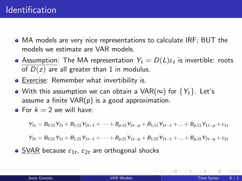
MA models are very nice representations to calculate IRF; BUT themodels we estimate are VAR models.

Assumption: The MA representation Yt = D(L)εt is invertible: rootsof D(z) are all greater than 1 in modulus.

Exercise: Remember what invertibility is.

With this assumption we can obtain a VAR(∞) for Yt. Let’sassume a finite VAR(p) is a good approximation.

For k = 2 we will have:

Y1t = B0,12Y2t +B1,12Y2t−1 + · · ·+Bp,12Y2t−p +B1,11Y1t−1 + ... +Bp,11Y1t−p + ε1t

Y2t = B0,21Y1t +B1,21Y1t−1 + · · ·+Bp,21Y1t−p +B1,22Y2t−1 + ... +Bp,22Y2t−p + ε2t

SVAR because ε1t , ε2t are orthogonal shocks


SVAR

Exercise: Discuss the problems you encounter trying to estimate theabove SVAR system by OLS

B(L)Yt = εt Structural VAR

Yt = B(L)−1εt = D(L)εt

B(L) = B0 − B1L− B2L2 − . . .− BpL

P

E (εtε′t) = Σε =

σ2

1 0 . . . 00 σ2

2 . . . 0...

.... . .

...0 0 . . . σ2

K

This SVAR has a reduced form (Sims(1980)) which is identified:Reduced form VAR(p): Yt = A1Yt−1 + . . . + ApYt−p + et

or A(L)Yt = etwhere A(L) = 1− A1L− . . .− ApL

P

innovations: et = Yt − Proj(Yt |Yt−1, . . . ,Yt−p),E (ete ′t) = Σe


Reduced form VAR

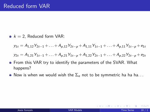
k = 2, Reduced form VAR:

y1t = A1,12Y2t−1 + . . .+Ap,12Y2t−p +A1,11Y1t−1 + . . .+Ap,11Y1t−p + e1t

y2t = A1,21Y1t−1 + . . .+Ap,21Y1t−p +A1,22Y2t−1 + . . .+Ap,22Y2t−p + e2t

From this VAR try to identify the parameters of the SVAR. Whathappens?

Now is when we would wish the Σe not to be symmetric ha ha ha. . .


Summary of VAR and SVAR notation

Reduced form VAR Structural VAR

A(L)Yt = et B(L)Yt = εtYt = A(L)−1et = C (L)et Yt = B(L)−1εt = D(L)εtA(L) = 1− A1L− A2L

2 − . . .− ApLp B(L) = B0 − B1L− . . .− BpL

p

E (ete ′t) = Σe(unrestricted) E (εt ε′t) = Σε =

σ2

1 0 . . . 00 σ2

2 . . . 0...

.... . .

...0 0 . . . σ2

K

Qet = εt , B(L) = QA(L), (B0 = Q), D(L) = C (L)Q−1

IRF:∂Yt+h

∂εt= Dh

Some remarks:1 A(L) is finite order p2 A(L), Σe , R are time invariant3 et spans the space of structural shocks εt , that is, εt = Qet

Question: When 3 doesn’t hold and how to solve the problem?Jesus Gonzalo VAR Models Time Series 11 / 1

Identification of shocks

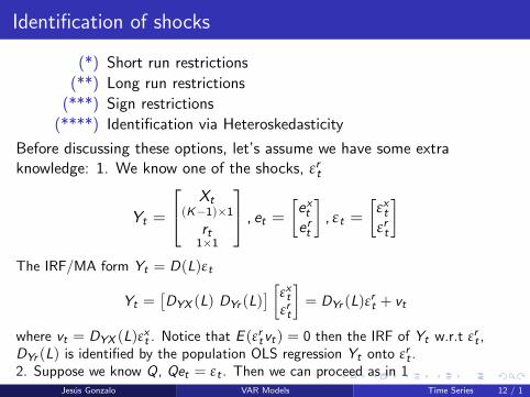
(*) Short run restrictions

(**) Long run restrictions

(***) Sign restrictions

(****) Identification via Heteroskedasticity

Before discussing these options, let’s assume we have some extraknowledge: 1. We know one of the shocks, εrt

Yt =

Xt(K−1)×1

rt1×1

, et =

[extert

], εt =

[εxtεrt

]The IRF/MA form Yt = D(L)εt

Yt =[DYX (L) DYr (L)

] [εxtεrt

]= DYr (L)ε

rt + vt

where vt = DYX (L)εxt . Notice that E (εrtvt) = 0 then the IRF of Yt w.r.t εrt ,

DYr (L) is identified by the population OLS regression Yt onto εrt .2. Suppose we know Q, Qet = εt . Then we can proceed as in 1



3. Suppose you have an IV zt (not in Yt) s.t:

i E (ztert ) 6= 0 (relevance)ii E (ztεxt ) = 0 (exogeneity)

Then you can estimate εrt and act as in 1. To show thispartion Yt

Yt =

[Xt

r rt

], et =

[extert

], εt =

[εxtεrt

]and Q =

[Qxx Qxr

Qrx Qrr

]so Qet = εt becomes:

Qxxext = −Qxre

rt + εxt

Qrrert = −Qrxe

xt + εrt

orext = −Q−1

xx Qxrert +Q−1

xx εxt (2)

ert = −Q−1rr Qrxe

xt +Q−1

rr εrt (3)



i Estimate −Q−1xx Qxr by IV estimation in (2)

ii Estimate εxt = Q−1xx εxt as εxt = ext + Q−1

xx Qxrert

iii Use εxt as instrument for ext in (3) to estimate −Q−1rr Qrx

iv Estimate εrt = Q−1rr εrt as ert + Q−1

rr Qrxext

v IRF as in (2) by regressing Yt on εrt , εrt−1,...

I don’t know why this IV approach has not been used more??? Anyanswer or comments???


Identification of shocksShort run restrictions

(*) Short Run Restrictions:YtK×1

= C (L) etK×1

; YtK×1

= D(L) εtK×1

Yt = Yt

C (L)et = D(L)εtC0et = D0εt or Qet = εt

so Q︸︷︷︸unknown

Σe︸︷︷︸known

Q ′ = Σε︸︷︷︸Diagonal

(4)

or Σe = D0ΣεD′0

There areK (K+1)

2 different equations in 4, so the order condition

says that we can estimate at mostK (K+1)

2 parameters. If we setΣε = I (a normalization), then we need:

K2 − K (K + 1)

2=

K (K − 1)

2restrictions on Q



Example: If K=2, then we need to impose a single restriction on Q,usually that Q is lower (Choleski) or upper triangular.

Instead of restrictions on Q you can think on restrictions on D0 (thisis why we call them short-run restrictions).

We could also have PARTIAL IDENTIFICATION where only a row ofQ is identified.Partion εt = Qet and Yt so that:[

εxtεrt

]=

[Qxx Qxr

Qrx Qrr

] [εxtεrt

]Suppose Qrx and Qrr are identified, then εrt can be computed andDyr (L) can be computed by regressing Yt on εrt , εrt−1,εrt−2,...



Some extra comment: The identification conditions discussed before(pure accounting) are “order conditions”. We should not forget therank conditions:r(Σε) = r(QΣeQ

′) (see Hamilton).Intuitively this restriction rules out that any column of Q can beexpressed as a linear combination of the others. While the rankcondition is typically important in large-scale simultaneous equationsystems, it is almost automatically satisfied in small scale VARs.


Identification of shocksLong run restrictions

(**) Long Run Restrictions:

Reduced form VAR: A(L)Yt = et (Yt = C (L)et)

Structural VAR: B(L)Yt = εt (Yt = D(L)εt)

LRV from VAR: Ω = A(1)−1Σe(A(1)−1)′ = C (1)ΣeC (1)′

LRV from SVAR: Ω = B(1)−1Σε(B(1)−1)′ = D(1)ΣεD(1)′

Notice that D(1) is the long-run effect on Yt of εt :

Yt = D(L)εt = (D(1) + (1− L) ˜D(L))εt︸︷︷︸Beveridge-Nelson decomposition

T

∑t=1

Yt = D(1)T

∑t=1

εt + εt − ε0



System identification by long-run restrictions: The SVAR is identifiedif:

A(1)−1Q−1Σε(Q−1)′A(1)−1 = Ω

K×K

or

D(1)ΣεD(1)′ = ΩK×K

(5)

can be solved for the unknown elements of Q and Σε (or D(1) andΣε)

Some accounting:

There are K (K+1)2 distinct equations in 5, so the order conditions say that

you can estimate (at most)K (K+1)

2 parameters. If we set Σε = I , it is clear

that we need K2 − K (K+1)2 = K (K−1)

2 restrictions on Q or D(1).



If K = 2, then K (K−1)2 = 1 which is delivered by imposing a single

exclusion restriction on Q or D(1) (for instance lower or uppertriangular).

If Σε = I then 5 can be rewritten:

Ω = D(1)D(1)′

If the zero restrictions on D(1) make D(1) lower triangular, thenD(1) is the Choleski factorization for Ω.



Example: Blanchard and Quah (1984)Goal to decompose GNP into permanent and transitory shocks. Theypostulate demand side shocks have only temporary effect on GNP whilesupply side shocks have permanent effect: ∆Yt

ut︸︷︷︸unemployment

=

[D11(L) D12(L)D21(L) D22(L)

] [εsεd

]E (εtε

′t) = I

•D12(1) = 0Estimate a VAR(p) [

A11(L) A12(L)A21(L) A22(L)

] [∆Yt

ut

]=

[e1t

e2t

]



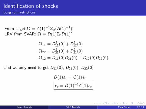
From it get Ω = A(1)−1Σe(A(1)−1)′

LRV from SVAR: Ω = D(1)ΣεD(1)′

Ω11 = D211(0) +D2

12(0)

Ω22 = D221(0) +D2

21(0)

Ω12 = D11(0)D21(0) +D12(0)D22(0)

and we only need to get D11(0), D21(0), D22(0)

D(1)εt = C (1)et

εt = D(1)−1C (1)et


Identification of shocksIdentification by Sign Restrictions

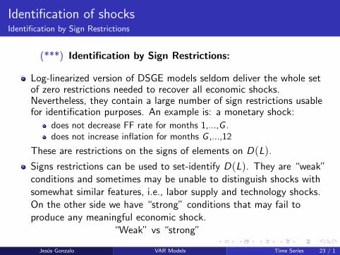
(***) Identification by Sign Restrictions:

Log-linearized version of DSGE models seldom deliver the whole setof zero restrictions needed to recover all economic shocks.Nevertheless, they contain a large number of sign restrictions usablefor identification purposes. An example is: a monetary shock:

does not decrease FF rate for months 1,...,G .does not increase inflation for months G ,...,12

These are restrictions on the signs of elements on D(L).

Signs restrictions can be used to set-identify D(L). They are “weak”conditions and sometimes may be unable to distinguish shocks withsomewhat similar features, i.e., labor supply and technology shocks.On the other side we have “strong” conditions that may fail toproduce any meaningful economic shock.

“Weak” vs “strong”


Identification of shocksBy Sign Restrictions

It is relatively complicated to impose sign restrictions on thecoefficients of the VAR as this requieres maximum likelihoodestimation of the full system under inequality constraints.

However, it is relatively easy to do it ex-post on IRF. For instance,following Canova and De Nicolo (2002):

1. Estimate A(L)Σe

2. Get orthogonal shocks without imposing zero restrictions:

Σe = P︸︷︷︸eigenvectors

V︸︷︷︸eigenvalues

P ′ = PP ′ = PRR ′P ′ s.t RR ′ = I

3. For each of the orthogonalized shocks one can check whether theidentifying restrictions are satisfied. If a shock is found the processterminates.

4. If we find more than one we could impose stronger conditions or takethe average of both shocks.


Identification of shocksFrom Heteroskedasticity, Rigobon (2003)

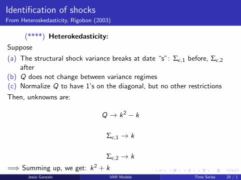
(****) Heterokedasticity:

Suppose

(a) The structural shock variance breaks at date “s”: Σε,1 before, Σε,2

after

(b) Q does not change between variance regimes

(c) Normalize Q to have 1’s on the diagonal, but no other restrictions

Then, unknowns are:

Q → k2 − k

Σε,1 → k

Σε,2 → k

=⇒ Summing up, we get: k2 + kJesus Gonzalo VAR Models Time Series 25 / 1

Identification of shocksFrom Heteroskedasticity, Rigobon (2003)

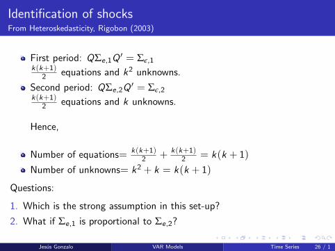
First period: QΣe,1Q′ = Σε,1

k(k+1)2 equations and k2 unknowns.

Second period: QΣe,2Q′ = Σε,2

k(k+1)2 equations and k unknowns.

Hence,

Number of equations= k(k+1)2 + k(k+1)

2 = k(k + 1)

Number of unknowns= k2 + k = k(k + 1)

Questions:

1. Which is the strong assumption in this set-up?

2. What if Σe,1 is proportional to Σe,2?


Some Asymptotic ResultsStability

VAR(1): yt = A1yt−1 + et = (1− A1L)−1et = At1y0 + ∑t−1

i=0 Ai1et−i

Result: If all eigenvalues of A1 have modulus less than 1, then thesequence Ai

1 i = 0, 1, . . . is absolutely summable and we call the VAR(1)STABLE. This condition is equivalent to:

|Ik − A1z | 6= 0 for |z | ≤ 1



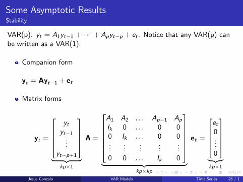
VAR(p): yt = A1yt−1 + · · ·+ Apyt−p + et . Notice that any VAR(p) canbe written as a VAR(1).

Companion form

yt = Ayt−1 + et

Matrix forms

yt =

ytyt−1

...yt−p+1

︸︷︷︸

kp×1

A =

A1 A2 . . . Ap−1 Ap

Ik 0 . . . 0 00 Ik . . . 0 0...

......

......

0 0 . . . Ik 0

︸︷︷︸

kp×kp

et =

et0...0

︸︷︷︸kp×1



Thus, yt is stable if |Ikp −Az | 6= 0 for |z | ≤ 1. Because,

|Ikp −Az | = (Ik − A1z − · · · − Apzp)

Then, the stability condition can be written as:

|Ik − A1z − · · · − Apzp | 6= 0 for |z | ≤ 1



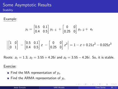
Example:

yt =

[0.5 0.10.4 0.5

]yt−1 +

[0 0

0.25 0

]yt−2 + et

∣∣∣∣[1 00 1

]−[

0.5 0.10.4 0.5

]z −

[0 0

0.25 0

]z2

∣∣∣∣ = 1− z + 0.21z2 − 0.025z3

Roots: z1 = 1.3; z2 = 3.55 + 4.26i and z3 = 3.55− 4.26i . So, it is stable.

Exercise:

Find the MA representation of yt .

Find the ARMA representation of yt .


Estimation (Least-Squares)

yt = A1yt−1 + · · ·+ Apyt−p + et

In simultaneous equations format: y = Bz + e

y =

y1...yT

︸︷︷︸T×K

B =[A1 · · · Ap

]︸︷︷︸K×(Kp)

zt =

yt...

yt−p+1

︸︷︷︸

p×K

Or, vec(y) = vec(Bz) + vec(e) = (z ′ ⊗ Ik)vec(B) + vec(e)

Or, y = (z ′ ⊗ Ik)β + vec(e) with β = vec(B).

=⇒ β =((z ′z)−1z ⊗ Ik

)y


Estimation (Least-Squares)Asymptotic properties

√T (β− β) =

√Tvec(B − B)

d−→ N(0, Γ−1 ⊗ Σe)

with Γ = p lim z ′zT .

It can also be proved that:

p lim Σe = p limee ′

T= Σe

Exercise: Show that if there are not restrictions on the VAR, OLSestimation of the parameters, equation by equation, is consistent andefficient.


Estimation (Least-Squares)Inference

From the asymptotic distribution of β it is straightforward to makeinference:

H0 : R︸︷︷︸N×k2

p

β = c vs. H1 : Rβ 6= c

√T (R β− Rβ)

d−→ N(0,R(Γ−1 ⊗ Σe)R′)

And hence,

T (R β− c)′[R(Γ−1 ⊗ Σe)R′]−1(R β− c)

d−→ X 2(N)

WALD-STATISTIC:

(R β− c)′[R((z ′z)−1 ⊗ Σe)R′]−1(R β− c)

d−→ X 2(N)


Granger CausalityGranger (1969)

Let yt = (z ′t x′t)′, zt(h|It) be the optimal (minimum MSE) h-step

predictor of the process zt given the information set It . The correspondingMSE will be denoted by Σz (h|It). The process xt is said to cause zt inGranger sense if:

Σz (h|It) < Σz (h|It − xt |s ≤ t)

with It − xt |s ≤ t be all the information except the past and present ofxt .


Characterization of Granger Causality

VAR: A(L)yt = et ; A(0) = I and E(ete ′t) = Σe

MA: yt = C (L)et ; C (0) = I

And let’s continue with yt = (z ′t x′t)′. Thus,

zt(1|ys |s ≤ t) = zt(1|zs |s ≤ t)

iff C12,i = 0 for i = 1, 2, . . . or, equivalently, A12,i = 0 for i = 1, 2, . . .In this situation, we say xt does not Granger cause zt .

Think on how to test for Granger causality.


Determining the VAR order

TESTING:

yt = A1yt−1 + · · ·+ AMyt−M + et

General to particular:

H10 : AM = 0 vs. H1

1 : AM 6= 0

H20 : AM−1 = 0 vs. H2

1 : AM−1 6= 0|AM = 0

...

HM0 : A1 = 0 vs. HM

1 : A1 6= 0|AM = · · · = A2 = 0

In this scheme, each null hypothesis is tested conditionally on theprevious ones being true. The procedure terminates and the VARorder is chosen accordingly, if one of the null hypothesis is rejected.

A big problem is how to calculate the type I error of the wholeprocedure.



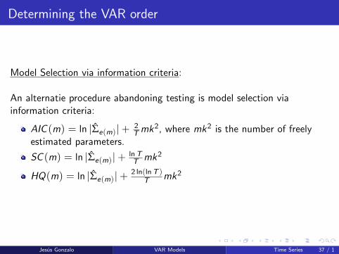
Model Selection via information criteria:

An alternatie procedure abandoning testing is model selection viainformation criteria:

AIC (m) = ln |Σe(m)|+ 2Tmk2, where mk2 is the number of freely

estimated parameters.

SC (m) = ln |Σe(m)|+ lnTT mk2

HQ(m) = ln |Σe(m)|+2 ln(lnT )

T mk2



Result:

yt︸︷︷︸k×1

∼ VAR(p); M ≥ p

And p is chosen so as to minimize a criterion:

IC (m) = ln |Σu(m)|+mCT

Tover m = 0, 1, . . . ,M

The estimate p is consistent iff:

CT → ∞ andCT

T→ 0 as T → ∞

And strongly consistent iff

CT

2 ln(lnT )> 1



Exercise: Which IC is consistent and which one is not?

Result:

limT→∞

Prob(p(AIC ) < p) = 0

and,

limT→∞

Prob(p(AIC ) > p) > 0

In a great paper, “Lag Length estimation in Large Dimensional Systems,JTSA”, Gonzalo and Pitarakis (2002) show that the latter probability goesto zero as k → ∞.


Impulse Response Function

Let’s consider a bivariate system yt = (y ′1t y′2t)′. Thus, the MA

representation yt = C (L)et is given by:

[y1t

y2t

]=

[e1t

e2t

]+

[C11,1 C12,1

C21,1 C22,1

] [e1t−1

e2t−1

]+

[C11,2 C12,2

C21,2 C22,s

] [e1t−2

e2t−2

]+ · · ·

Impulse Response Function: For i = 1, 2, it is the effect of a unitchange in eit in yit+s ≈ dynamic multiplier. That is,

∂y1t+s

∂e1t= ψ11,s

∂y1t+s

∂e2t= ψ12,s

∂y2t+s

∂e1t= ψ21,s

∂y2t+s

∂e2t= ψ22,s


Impulse Response Function

Notice that there is a serious problem on interpreting these partialderivatives because e1t and e2t are correlated. This is one of the reasonsto orthogonalize shocks.

Exercise: In the bivariate case, using OLS, get orthogonal shocks from(e ′1t e

′2t)′.


IRF with orthogonal shocks

E(ete ′t) = Σe ; pick a matrix Q such that: QΣeQ′ = I . Thus,

yt = C (L)Q−1Qet = D(L)εt ; Qet = εt

[y1t+s

y2t+s

]=

[D11,0 D12,0

D21,0 D22,0

] [ε1t+s

ε2t+s

]+ · · ·+

[D11,s D12,s

D21,s D22,s

] [ε1t

ε2t

]+ · · ·+

∂y1t+s

∂ε1t= D11,s

∂y1t+s

∂ε2t= D12,s

∂y1t+s

∂ε1t= D11,s

∂y1t+s

∂ε2t= D12,s


IRF with orthogonal shocks

So, we have four IRF for the bivariate case:

Plot D11,s vs. ”s” (ε1t shocks on y1t)




Long-run effects on each shock on y1t

and y2t are:

(1)∞

∑s=0

D11,s (2)∞

∑s=0

D12,s

(3)∞

∑s=0

D21,s (4)∞

∑s=0

D22,s


Variance decompositions

Goal: To determine the proportion of the variability of y1t+s , y2t+s that isdue to the shocks ε1t and ε2t . This allows us to determine the relativeimportance of the exogenous shocks to the evolution of y1t and y2t .

The Forecast error (FE) is given by:

FE (s) = yt+s − E[yt+s |It ] = D0εt+s +D1εt+s−1 + · · ·+Ds−1εt+1

Or, [y1t+s

y2t+s

]−[

E(y1t+s |It)E(y2t+s |It)

]=

[D11,0 D12,0

D21,0 D22,0

] [ε1t+s

ε2t+s

]+

+

[D11,1 D12,1

D21,1 D22,1

] [ε1t+s−1

ε2t+s−1

]+ · · ·+

[D11,s−1 D12,s−1

D21,s−1 D22,s−1

] [ε1t+1

ε2t+1

]Jesus Gonzalo VAR Models Time Series 44 / 1


Focusing on the first equation:

y1t+s − E(y1t+s |It) = D11,0ε1t+s + · · ·+D11,s−1ε1t+1

+D12,0ε2t+s + · · ·+D12,s−1ε2t+1

Thus,

MSE = E [y1t+s − E(y1t+s |It)]2 = δ21(s)

= δ21(D

211,0 +D2

11,1 + · · ·+D211,s−1)

+ δ22(D

212,0 +D2

12,1 + · · ·+D212,s−1)



The proportion of δ21(s) due to shocks in ε1t is:

P11(s) =δ2

1(D211,0 +D2

11,1 + · · ·+D211,s−1)

δ21(s)

due to ε2t is:

P12(s) =δ2

2(D212,0 +D2

12,1 + · · ·+D212,s−1)

δ21(s)

and similarly, for P21(s) and P22(s)



The previous results are reported usually in the following way:

s MSE P11(s) P12(s)

1 .0084 100% 0%

2 .0089 99% 1%

3 .0092 98.5% 1.5%

4 .0093 98.1% 1.9%


Confidence intervals for IRF

1. δ-method

2. Bootstrap methods

3. Monte-Carlo methods

4. Bayesian Methods

We will only discuss the first two.


Confidence intervals for IRFδ-method

Remember the “delta” method:

If√T (θ − θ0)

d∼ N(0, Σθ) and if g(·) has continuous derivatives then

√T(g(θ)− g(θ0)

)≈√T

∂g

∂θ

∣∣∣∣θ0

(θ − θ0)d∼ N

(0,

∂g

∂θ

∣∣∣∣θ0

Σθ

∂g

∂θ

∣∣∣∣θ0

)

For SVAR IRFs:

θ = (A(L),Q) and g(θ) = D(L) = A(L)−1Q


Confidence intervals for IRFδ-method

Problems:

(i) g(·) is very non-linear so then even if A(L) were exactly normallydistributed the IRF may not be. Let β ∼ N(0.25, 1), which is thedistribution of β4 or 1

β?

(ii) A(L) is not real approximated by a normal if roots are large.


Confidence intervals for IRFBootstrap methods

Algorithm:

(i.) Obtain VAR estimates A(L), et .

(ii.) Obtain e l via bootstrap and construct A(L)y lt = e lt , for l = 1, . . . , L.

(iii.) Estimate Al (L) by using data constructed in the previous apart.Compute D l (L).

(iv.) Report percentiles of the distribution of Dj .

Remarks:

et should be white noise. Serious problems when it shows correlationsand/or heteroskedasticity.

Problem when there is a large persistence because then VARcoefficients usually are downward biased.


(+) & (-) of VAR models

(-)

Time aggregation

Large dimension

Sometimes we have VAR(∞)

Construction of confidence bands for the IRF

(+)

They require very little to be used. This is just the opposite thanDSGE models. Notice that people use VAR models to check DSGEresults.


VAR Models Jesus Gonzalo - UC3Mjgonzalo/teaching/PhdTimeSeries/VAR models 2017.pdfVAR Models Jesus...

Documents

Transcript of VAR Models Jesus Gonzalo - UC3Mjgonzalo/teaching/PhdTimeSeries/VAR models 2017.pdfVAR Models Jesus...