1

Vapour-liquid equilibria of the CH4 + CO2 + H2S ternary

system with two different global compositions: experiments

and modelling

Pascal Theveneau1, Xiaochun Xu

2, Olivier Baudouin

3, Jean-Noël Jaubert

2, Paola Ceragioli

4,

Christophe Coquelet1*

1MINES ParisTech, PSL Université, CTP- Centre Thermodynamique des Procédés, 35 rue Saint Honoré, 77300

Fontainebleau France

2Université de Lorraine, École Nationale Supérieure des Industries Chimiques, Laboratoire Réactions et Génie des

Procédés (UMR CNRS 7274), 1 rue Grandville, 54000, Nancy, France

3ProSim SA, Immeuble Stratège A, 51 rue Ampère, 31670 Labège, France

4Eni UPS, Via Maritano 26, 20097 San Donato Milanese, Milano, Italy

Abstract

The vapor-liquid equilibrium for two mixtures containing methane, carbon dioxide and hydrogen

sulphide was determined experimentally by a static-analytic method. Thirty-one data points were

acquired for a range of temperatures from 243 K to 333 K at pressures up to 11 MPa. The measured

data were correlated with the Peng Robinson equation of state (EoS) and different mixing rules,

which led to the conclusion that a cubic EoS could simultaneously predict the existence of a 3-phase

region and 2 critical points on the constant-composition two-phase boundary curve.

Key words: Equation of state, Static-analytic method, data treatment, gas processing

(*) author to whom correspondence should be addressed

E-mail: christophe.coquelet@mines-paristech.fr

Tel: +33 164694968 Fax: +33 164694968

2

Introduction

In the context of energetic transition, it appears that natural gas could be the best replacement for

oil or coal. Natural gas is usually composed of methane and other hydrocarbons, but in recent

decades, a number of sour natural gas sources and gas-condensate fields have been discovered

around the world. Some of them contain large amounts of sulphur compounds, such as hydrogen

sulphide, together with carbon dioxide1. Therefore, the oil and gas industry requires vapour-liquid

equilibrium data for mixtures containing methane + hydrogen sulphide + carbon dioxide to develop

accurate models for calculating the thermodynamic properties of these complex natural gases. The

expected final result is an equation of state (EoS) that could be used to determine the phase

diagram, the compressibility and the density of sour natural gases within large temperature and

pressure ranges.

To obtain accurate results with an EoS, the molecular interactions between the different components

of a mixture must be characterized. Such characterization is usually performed through the

definition of the mixing and combining rules2 for the parameters of the EoS. The combining rules

typically require the determination of the binary interaction parameters (BIPs), which can be either

fitted based on experimental data or estimated by group-contribution methods such as those used in

the PPR783,4

, PR2SRK5 and PSRK

6 predictive thermodynamic models.

The ternary system CH4 + CO2 + H2S is composed of 3 binary systems that must be analysed.

Many experimental data are available for the binary system CH4 + CO27–19

which can be classified

as a type I system according to the classification scheme of van Konynenburg and Scott20,21

. Due to

the value of the melting temperature of CO2, a solid-liquid-vapor equilibrium may appear at

temperatures higher than the critical temperature of CH422

. The binary system CO2 + H2S, which is

also a type I system, was studied in our research laboratory (CTP) in 2013. The vapour–liquid

equilibrium data we measured were published in Chapoy et al.23

and were found to be in good

agreement with existing data in the literature about the same binary system. The last binary system,

CH4 + H2S, was also previously studied by our research group (in 2014) because it is a key system

for the development of the SPREX H2S process24

. It can be classified as a type III system according

to the classification scheme of van Konynenburg and Scott, meaning that at low temperature, the

system exhibits vapour-liquid-liquid equilibria. Due to its complexity, such a system was used as an

example by Heidemann and Khalil25

to describe the computation of the mixture critical line for type

III systems. In 1999, Bluma and Deiters26

proposed a classification scheme for phase diagrams of

ternary fluid systems. As previously stated, the studied ternary system (CH4 + CO2 + H2S) contains

one type III binary subsystem and two type I binary subsystems. According to Bluma and Deiters,

such a configuration corresponds to a type III ternary system (denoted T-III). Moreover, phase

equilibria measurements were performed with such a ternary system by Ng et al.27,28

who

3

highlighted the existence of a vapour-liquid-liquid equilibrium region and confirmed the type of the

ternary system.

In this paper, new vapour-liquid equilibrium data are presented for two different global

compositions of the ternary system. The experimental method used in this work is a static-analytic

type method. This method takes advantage of a capillary sampler (ROLSI®, Armines’ patent)

developed in the CTP laboratory. Table 1 presents the composition of the 2 studied mixtures, which

were purchased from Air Products, along with the corresponding uncertainties. These 2 mixtures

were also analysed by gas chromatography in the CTP laboratory, and the results of this analysis

can be found in Table 1.

[Table 1]

The measured data were correlated with the Peng-Robinson29,30

(PR) equation of state (EoS)

combined with the Wong-Sandler mixing rules31

. The cubic EoS was used without volume

translation32–34

because this work focuses only on fluid phase equilibria calculations. Meanwhile,

the PPR783,35

model was applied for predicting the vapor-liquid equilibrium (VLE) and phase

boundaries of the ternary system.

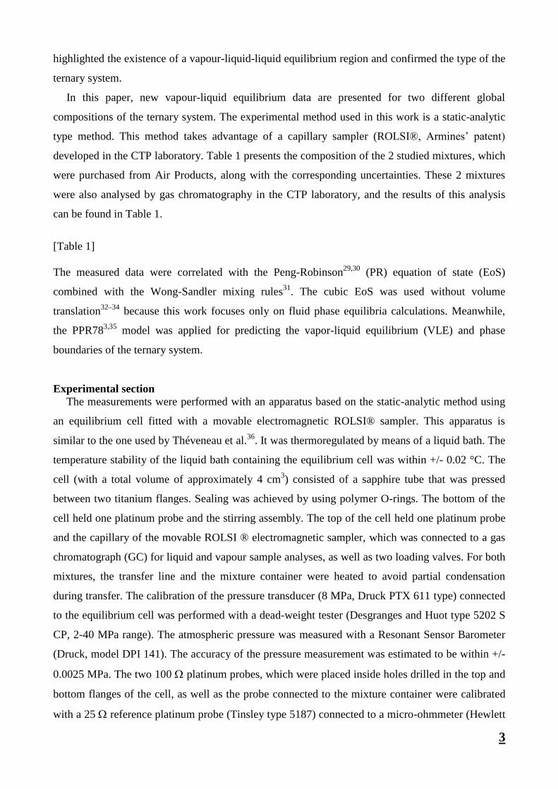
Experimental section

The measurements were performed with an apparatus based on the static-analytic method using

an equilibrium cell fitted with a movable electromagnetic ROLSI® sampler. This apparatus is

similar to the one used by Théveneau et al.36

. It was thermoregulated by means of a liquid bath. The

temperature stability of the liquid bath containing the equilibrium cell was within +/- 0.02 °C. The

cell (with a total volume of approximately 4 cm3) consisted of a sapphire tube that was pressed

between two titanium flanges. Sealing was achieved by using polymer O-rings. The bottom of the

cell held one platinum probe and the stirring assembly. The top of the cell held one platinum probe

and the capillary of the movable ROLSI ® electromagnetic sampler, which was connected to a gas

chromatograph (GC) for liquid and vapour sample analyses, as well as two loading valves. For both

mixtures, the transfer line and the mixture container were heated to avoid partial condensation

during transfer. The calibration of the pressure transducer (8 MPa, Druck PTX 611 type) connected

to the equilibrium cell was performed with a dead-weight tester (Desgranges and Huot type 5202 S

CP, 2-40 MPa range). The atmospheric pressure was measured with a Resonant Sensor Barometer

(Druck, model DPI 141). The accuracy of the pressure measurement was estimated to be within +/-

0.0025 MPa. The two 100 platinum probes, which were placed inside holes drilled in the top and

bottom flanges of the cell, as well as the probe connected to the mixture container were calibrated

with a 25 reference platinum probe (Tinsley type 5187) connected to a micro-ohmmeter (Hewlett

4

Packard 34420A). The reference probe was calibrated by LNE (Paris) according to the ITS 90 scale.

The accuracy of the temperature measurement was estimated to be within +/- 0.025 °C. GC

analyses were performed using a gas chromatograph (Varian, model 3800) fitted with a thermal

conductivity detector (TCD). The analytical column was a Porapack Q packed column (2 metres in

length, 1/8” wide, 100/120 mesh) thermostated at 40 °C in the GC oven. Known volumes of pure

methane, carbon dioxide and hydrogen sulphide were directly injected into the injector of the gas

chromatograph by using calibrated airtight syringes of various volumes. Calibration curves showing

the “component peak area versus the component mole number” appeared to be linear within the

experimental uncertainties. The mean relative accuracy of the measurement of the experimental

mole number was estimated to be within +/- 2 % for CH4, +/- 1.5 % for CO2 and +/- 2 % for H2S.

When the pressure and temperature were constant in the cell, each phase was analysed by gas

chromatography using the movable electromagnetic ROLSI® sampler. Generally, no more than

three samplings were necessary to purge the capillary and to obtain representative samples of the

mixture at equilibrium. Approximately five to ten samples were obtained from each phase for

composition determination. As highlighted by Eq. (1), the uncertainty in the composition can be

calculated based on the knowledge of the uncertainty of each mole number:

ncomp

i

i

i

i

i nun

xxu

ji

2

2

(1)

For a binary system, one obtains:

2

2

2

2

1

1111 1

n

nu

n

nuxxxu (2)

For a ternary system, one obtains:

2

3

32

3

2

2

22

2

2

1

12

111 1

n

nux

n

nux

n

nuxxxu (3)

The maximum uncertainty in the mole fraction was found to be u(z)=0.007.

Experimental results

Tables 2 and 3 present the measured vapour-liquid equilibrium data for mixtures 1 and 2,

respectively. The global composition of each mixture can be found in Table 1.

[Table 2]

[Table 3]

5

6

Data treatment

All the experimental data were correlated with Simulis Thermodynamics software, which was

developed by ProSim SA. The Peng Robinson EoS with different mixing rules was chosen because

of its simplicity and its widespread utilization in chemical engineering. Its formulation is:

ca TRTp

v b v v b b v b

(4)

The critical temperature (Tc) and critical pressure (pc) used for estimating b and ac are given in

Table 4 for each pure compound. The acentric factor () used in the PPR78 model is also reported.

In this paper, two different mixing rules were successively used to correlate the experimental data

measured in this study. In the first analysis, the Wong-Sandler (WS) mixing rules were used, and in

the second analysis, classical van der Waals mixing rules combined with a group contribution

method to estimate the BIPS (the so-called PPR78 model) were used.

Correlation of the measured data with the PR EoS and WS mixing rules.

In this paper, to accurately predict the vapor pressures of each component, the WS mixing rules are

used in conjunction with a specific alpha function, namely, the Mathias-Copeman alpha function37

.

This function, given below, was developed especially for polar compounds and has three adjustable

parameters. Although it is non-consistent38–40

, its accuracy has been demonstrated.

If T<Tc,

23

3

2

21 1111

CCC T

Tc

T

Tc

T

TcT (5)

If T>Tc,

2

1 11

CT

TcT (6)

The component-dependent c1, c2 and c3 parameters are given in Table 4. They originate from Reid

et al.41

[Table 4]

The WS mixing rules31

are written as follows:

7

1 1

1

1

(1 )2

( , )( )

1

( )( , ) ( )

2For the PR EoS: ln 1 2 0.6232

2

jip p i j

i j ij

i j

pEi

iEoS ii

p Ei

ii EoSi

EoS

aab b

RT RTx x k

b Ta T

xRTC RTb

a Ta T b x

b C

C

x

x x

G

G

(7)

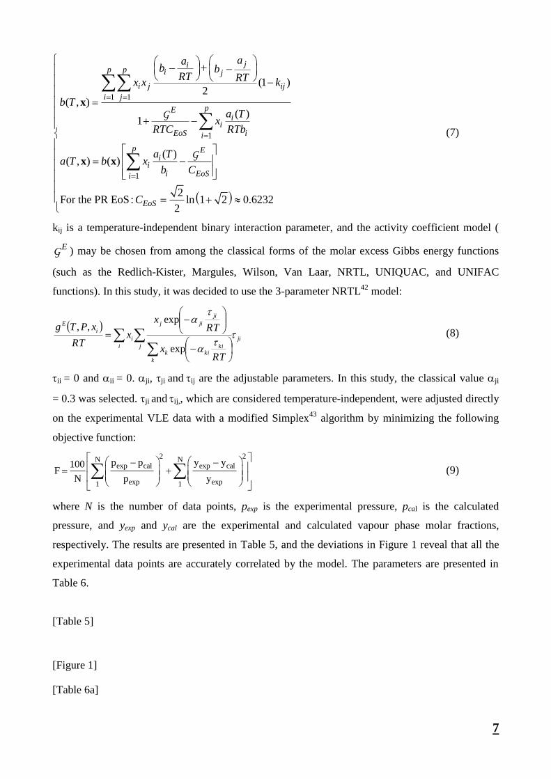
kij is a temperature-independent binary interaction parameter, and the activity coefficient model (

EG ) may be chosen from among the classical forms of the molar excess Gibbs energy functions

(such as the Redlich-Kister, Margules, Wilson, Van Laar, NRTL, UNIQUAC, and UNIFAC

functions). In this study, it was decided to use the 3-parameter NRTL42

model:

ji

i j

k

kikik

ji

jij

i

i

E

RTx

RTx

xRT

xPTg

exp

exp,,

(8)

ii = 0 and ii = 0. ji, ji and ij are the adjustable parameters. In this study, the classical value ji

= 0.3 was selected. ji and ij,, which are considered temperature-independent, were adjusted directly

on the experimental VLE data with a modified Simplex43

algorithm by minimizing the following

objective function:

2 2N Nexp cal exp cal

exp exp1 1

p p y y100F

N p y

(9)

where N is the number of data points, pexp is the experimental pressure, pcal is the calculated

pressure, and yexp and ycal are the experimental and calculated vapour phase molar fractions,

respectively. The results are presented in Table 5, and the deviations in Figure 1 reveal that all the

experimental data points are accurately correlated by the model. The parameters are presented in

Table 6.

[Table 5]

[Figure 1]

[Table 6a]

8

[Table 6b]

Accuracy of the WS mixing rules used to correlate other literature data.

In 1985, Ng et al.27,28

published some data on the same ternary system examined in this study with

different global composition (CH4: 0.4988, CO2: 0.0987, H2S: 0.4022). Using the PR EoS combined

with the WS mixing rules and the parameters that were adjusted based on the data measured in this

paper, a bubble-point algorithm was used to predict the data obtained by Ng et al. The deviations

are shown in Table 7 and Figure 2. They are dispersed, but on average, the data were accurately

predicted within the temperature range in which the parameters were fitted. Outside of the

temperature range in which our data were acquired, the deviations are higher.

[Table 7]

[Figure 2]

Correlation of the measured data and other literature data with the PPR78 model

In this section, the application of the PPR78 model3,44,45

to predict the VLE properties and the phase

behaviour of the CH4-CO2-H2S system is discussed. Such a model combines the well-established

PR-EoS (with the Soave46

alpha function) and a group-contribution method to estimate the

temperature-dependent binary interaction parameters, kijPR

(T), which appear in the equations

derived from the classical Van der Waals one−fluid mixing rules:

N NPR

i j i j ij

i=1 j=1

N

i i

i=1

a = x x a (T)×a (T) 1 k (T)

b = x b

(10)

and,

klg g

kl

B 2N N 1A ji

ik jk il jl kli jk 1 l 1

PRij

i j

i j

a (T)a (T)1 298.15( )( )A

2 T K b b

k (T)a (T) a (T)

2b b

(11)

The Ng variable represents the number of different groups defined according to the group-

contribution method. The αik variable represents the fraction of molecule i occupied by group k

(occurrence of group k in molecule i divided by the total number of groups present in molecule i).

9

The group-interaction parameters Akl = Alk and Bkl = Blk (where k and l are two different groups)

were determined during the development of the model. Those parameters that are needed to perform

the calculations for the ternary system CH4/CO2/H2S are shown in Table 8.

[Table 8]

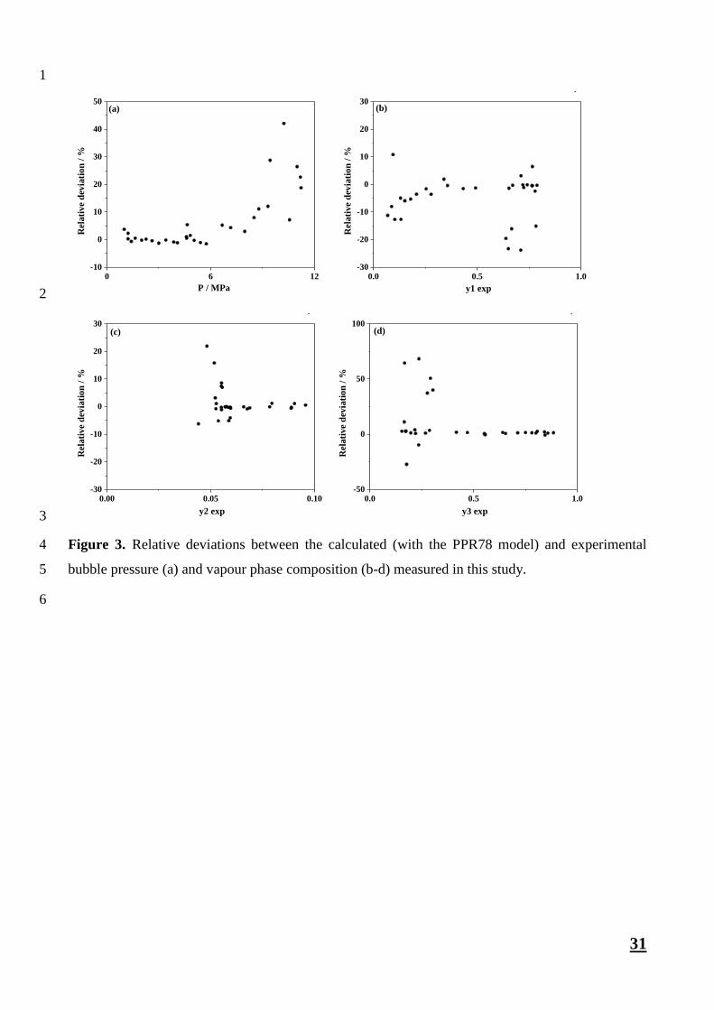
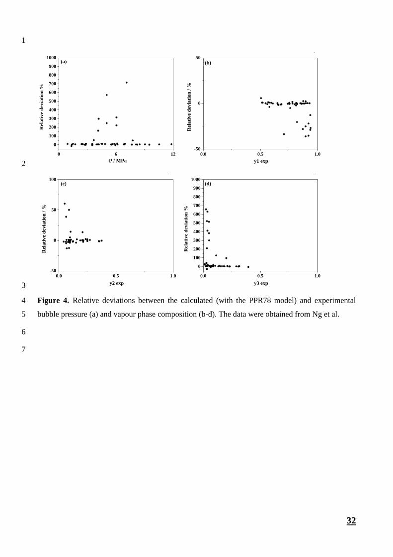
The deviations between the experimental VLE data and the predictions of the PPR78 model for

both the data measured in this study and those measured by Ng et al.27,28

are shown in Figure 3 and

Figure 4, respectively. As shown in these figures, the deviations were satisfactory (<10 %) for most

cases. However, the deviations may become very high, especially when the slope of the bubble

curve becomes very steep at low temperatures (a small change in temperature greatly changes the

bubble pressure).

[Figure 3]

[Figure 4]

Prediction of the (P,T) envelopes with the PR EoS and different mixing rules

Meanwhile, the PPR78 model and the PR EoS combined with the WS mixing rules were applied to

predicting the PT envelopes of the ternary CH4-CO2-H2S mixture with different fixed global

compositions. It was decided to perform the calculations according to the two global compositions

studied in this paper and the global composition reported by Ng et al.27

As explained by the authors,

this ternary system (with the composition they studied) exhibits a very narrow three-phase region at

lower temperatures. The two-phase boundary curve commences at a dew point locus that passes

through an upper retrograde region and terminates at a vapour-liquid critical point. The phase

boundary then follows a bubble point locus that terminates at a liquid-liquid critical point. After

this, the boundary turns sharply upward at higher pressures and lower temperatures and separates

the single phase from the liquid-liquid region. As shown in Figure 5, the PPR78 model can

reproduce these complex phase behaviours for the mixture and accurately predict the three-phase

equilibrium region. As previously discussed, the CH4-CO2 mixture and the CO2-H2S mixture

belong to the type I system, whereas the CH4-H2S mixture is a type III system according to the

classification scheme of Van Konynenburg and Scott. As discussed in the literature47

, cubic

equations of state based on van der Waals-type mixing rules with only one binary interaction

parameter present difficulties for modelling the critical loci of type III systems. Indeed, at least two

binary interaction parameters are needed for the modelling of these systems. It is thus not surprising

to observe that the PPR78 model is not able to locate the two critical points at the right places on the

boundary curve. The results obtained with the WS mixing rules are shown in Figure 6, which makes

10

it possible to conclude that the selected mixing rules accurately predict the cricondentherm and

cricondenbar but do not predict the existence of the two critical points.

The phase boundaries of two mixtures reported in this work that were predicted with the PPR78

model and the PR EoS with the WS mixing rules are presented in Figures 7 and 8, respectively. For

mixture 1, a classical PT envelope that included a dew-point curve and a bubble-point curve was

obtained, and the 2 models showed very comparable results (see Figures 7a and 7b). For mixture 2,

a PT envelope similar to the one reported by Ng et al. was obtained. However, for the global

composition, the PPR78 model was unable to predict the existence of the bubble curve and

consequently the existence of the 2 critical points. However, the PR EoS with the WS mixing rules

predicted the correct topology of the phase envelope.

[Figure 5]

[Figure 6]

[Figure 7]

[Figure 8]

Conclusion

New experimental vapor-liquid equilibrium data were acquired for the ternary CH4 + CO2 + H2S

system at temperatures between 243 and 333 K (U(T)=0.03 K) and at pressures up to 11 MPa

(U(p)=0.003 MPa) with a Umax(z)=0.007. With the aid of the software Simulis Thermodynamics,

the data could be accurately correlated with the Peng Robinson EoS combined with the Wong

Sandler mixing rules and the NRTL activity coefficient model. Such a thermodynamic model was

also used to correlate the data published by Ng et al., and the deviations were found to be acceptable

within the range of temperatures in which the parameters were fitted, i.e., within the temperature

range in which the experiments were performed.

The predictive PPR78 model, which is available in Simulis Thermodynamics, was also used to

predict the same data. The resulting deviations were satisfactory in most cases but were very high

when the slope of the bubble curve was very steep at low temperatures.

In the end, both models were used to predict the PT envelopes of the ternary CH4-CO2-H2S

mixture with different fixed global compositions. Both models succeeded in predicting the

existence of a 3-phase region and the 2 critical points.

11

Acknowledgements

Ing. Pascal Théveneau and Professor Christophe Coquelet would like to thank Professor Dominique

Richon for fruitful discussions.

References

(1) Hajiw, M. Hydrate Mitigation in Sour and Acid Gases, Mines ParisTech, 2014.

(2) Sandler, S. I.; Orbey, H. Mixing and Combining Rules. In Equations of state for fluids and

fluid mixtures. Part I.; Experimental thermodynamics; Elsevier: Amsterdam ; New York,

2000; pp 321–358.

(3) Jaubert, J.-N.; Mutelet, F. VLE Predictions with the Peng-Robinson Equation of State and

Temperature-Dependent kij Calculated through a Group Contribution Method. Fluid Phase

Equilibria 2004, 224 (2), 285–304.

(4) Xu, X.; Jaubert, J.-N.; Privat, R.; Arpentinier, P. Prediction of Thermodynamic Properties of

Alkyne-Containing Mixtures with the E-PPR78 Model. Ind. Eng. Chem. Res. 2017, 56 (28),

8143–8157.

(5) Jaubert, J.-N.; Privat, R. Relationship between the Binary Interaction Parameters (kij) of the

Peng–Robinson and Those of the Soave–Redlich–Kwong Equations of State: Application to

the Definition of the PR2SRK Model. Fluid Phase Equilibria 2010, 295 (1), 26–37.

(6) Holderbaum, T.; Gmehling, J. PSRK: A Group Contribution Equation of State Based on

UNIFAC. Fluid Phase Equilibria 1991, 70 (2–3), 251–265.

(7) Bian, B.; Wang, Y.; Shi, J.; Zhao, E.; Lu, B. C.-Y. Simultaneous Determination of Vapor-

Liquid Equilibrium and Molar Volumes for Coexisting Phases up to the Critical Temperature

with a Static Method. Fluid Phase Equilibria 1993, 90 (1), 177–187.

(8) Al-Sahhaf, T. A.; Kidnay, A. J.; Sloan, E. D. Liquid + Vapor Equilibriums in the Nitrogen +

Carbon Dioxide + Methane System. Ind. Eng. Chem. Fundam. 1983, 22 (4), 372–380.

(9) Knapp, H.; Yang, X.; Zhang, Z. Vapor—Liquid Equilibria in Ternary Mixtures Containing

Nitrogen, Methane, Ethane and Carbondioxide at Low Temperatures and High Pressures.

Fluid Phase Equilibria 1990, 54, 1–18.

(10) Wei, M. S.-W.; Brown, T. S.; Kidnay, A. J.; Sloan, E. D. Vapor + Liquid Equilibria for the

Ternary System Methane + Ethane + Carbon Dioxide at 230 K and Its Constituent Binaries at

Temperatures from 207 to 270 K. J. Chem. Eng. Data 1995, 40 (4), 726–731.

(11) Xu, N.; Dong, J.; Wang, Y.; Shi, J. High Pressure Vapor Liquid Equilibria at 293 K for

Systems Containing Nitrogen, Methane and Carbon Dioxide. Fluid Phase Equilibria 1992, 81,

175–186.

(12) Arai, Y.; Kaminishi, G.-I.; Saito, S. The Experimental Determination Of The P-V-T-X

Relations For The Carbon Dioxide-Nitrogen And The Carbon Dioxide-Methane Systems. J.

Chem. Eng. Jpn. 1971, 4 (2), 113–122.

(13) Davalos, J.; Anderson, W. R.; Phelps, R. E.; Kidnay, A. J. Liquid-Vapor Equilibria at 250.00K

for Systems Containing Methane, Ethane, and Carbon Dioxide. J. Chem. Eng. Data 1976, 21

(1), 81–84.

(14) Webster, L. A.; Kidnay, A. J. Vapor−Liquid Equilibria for the Methane−Propane−Carbon

Dioxide Systems at 230 K and 270 K. J. Chem. Eng. Data 2001, 46 (3), 759–764.

(15) Mraw, S. C.; Hwang, S.-C.; Kobayashi, R. Vapor-Liquid Equilibrium of the Methane-Carbon

Dioxide System at Low Temperatures. J. Chem. Eng. Data 1978, 23 (2), 135–139.

(16) Donnelly, H. G.; Katz, D. L. Phase Equilibria in the Carbon Dioxide–Methane System. Ind.

Eng. Chem. 1954, 46 (3), 511–517.

(17) Somait, F. A.; Kidnay, A. J. Liquid-Vapor Equilibriums at 270.00 K for Systems Containing

Nitrogen, Methane, and Carbon Dioxide. J. Chem. Eng. Data 1978, 23 (4), 301–305.

(18) Kaminishi, G.-I.; Arai, Y.; Saito, S.; Maeda, S. Vapor-Liquid Equilibria For Binary And

Ternary Systems Containing Carbon Dioxide. J. Chem. Eng. Jpn. 1968, 1 (2), 109–116.

12

(19) Neumann, A.; Walch, W. Dampf/Flüssigkeits-Gleichgewicht CO2/CH4 im Bereich tiefer

Temperaturen und kleiner CO2-Molenbrüche. Chem. Ing. Tech. 1968, 40 (5), 241–244.

(20) Van Konynenburg, P. H.; Scott, R. L. Critical Lines and Phase Equilibria in Binary Van Der

Waals Mixtures. Philos. Trans. R. Soc. Math. Phys. Eng. Sci. 1980, 298 (1442), 495–540.

(21) Privat, R.; Jaubert, J.-N. Classification of Global Fluid-Phase Equilibrium Behaviors in Binary

Systems. Chem. Eng. Res. Des. 2013, 91 (10), 1807–1839.

(22) Stringari, P.; Campestrini, M.; Coquelet, C.; Arpentinier, P. An Equation of State for Solid–

Liquid–Vapor Equilibrium Applied to Gas Processing and Natural Gas Liquefaction. Fluid

Phase Equilibria 2014, 362, 258–267.

(23) Chapoy, A.; Coquelet, C.; Liu, H.; Valtz, A.; Tohidi, B. Vapour–Liquid Equilibrium Data for

the Hydrogen Sulphide (H2S)+carbon Dioxide (CO2) System at Temperatures from 258 to

313K. Fluid Phase Equilibria 2013, 356, 223–228.

(24) Coquelet, C.; Valtz, A.; Stringari, P.; Popovic, M.; Richon, D.; Mougin, P. Phase Equilibrium

Data for the Hydrogen Sulphide+methane System at Temperatures from 186 to 313K and

Pressures up to about 14MPa. Fluid Phase Equilibria 2014, 383, 94–99.

(25) Heidemann, R. A.; Khalil, A. M. The Calculation of Critical Points. AIChE J. 1980, 26 (5),

769–779.

(26) Bluma, M.; Deiters, U. K. A Classification of Phase Diagrams of Ternary Fluid Systems.

Phys. Chem. Chem. Phys. 1999, 1 (18), 4307–4313.

(27) Ng, H.-J.; B. Robinson, D.; Leu, A.-D. Critical Phenomena in a Mixture of Methane, Carbon

Dioxide and Hydrogen Sulfide. Fluid Phase Equilibria 1985, 19 (3), 273–286.

(28) Robinson, D. B.; Ng, H.-J.; Leu, A. D. Behavior of CH4-CO2-H2S Mixtures at Sub-Ambient

Temperatures (RR-47). Res. Rep. GPA 1981, 1–38.

(29) Peng, D.-Y.; Robinson, D. B. A New Two-Constant Equation of State. Ind. Eng. Chem.

Fundam. 1976, 15 (1), 59–64.

(30) Pina-Martinez, A.; Privat, R.; Jaubert, J.-N.; Peng, D.-Y. Updated Versions of the Generalized

Soave α-Function Suitable for the Redlich-Kwong and Peng-Robinson Equations of State.

Fluid Phase Equilibria 2019, 485, 264–269.

(31) Wong, D. S. H.; Sandler, S. I. A Theoretically Correct Mixing Rule for Cubic Equations of

State. AIChE J. 1992, 38 (5), 671–680.

(32) Péneloux, A.; Rauzy, E.; Freze, R. A Consistent Correction for Redlich-Kwong-Soave

Volumes. Fluid Phase Equilibria 1982, 8 (1), 7–23.

(33) Jaubert, J.-N.; Privat, R.; Le Guennec, Y.; Coniglio, L. Note on the Properties Altered by

Application of a Péneloux-Type Volume Translation to an Equation of State. Fluid Phase

Equilibria 2016, 419, 88–95.

(34) Privat, R.; Jaubert, J.-N.; Le Guennec, Y. Incorporation of a Volume Translation in an

Equation of State for Fluid Mixtures: Which Combining Rule? Which Effect on Properties of

Mixing? Fluid Phase Equilibria 2016, 427, 414–420.

(35) Qian, J.-W.; Jaubert, J.-N.; Privat, R. Phase Equilibria in Hydrogen-Containing Binary

Systems Modeled with the Peng-Robinson Equation of State and Temperature-Dependent

Binary Interaction Parameters Calculated through a Group-Contribution Method. J. Supercrit.

Fluids 2013, 75, 58–71.

(36) Théveneau, P.; Coquelet, C.; Richon, D. Vapour–Liquid Equilibrium Data for the Hydrogen

Sulphide+n-Heptane System at Temperatures from 293.25 to 373.22 K and Pressures up to

about 6.9 MPa. Fluid Phase Equilibria 2006, 249 (1–2), 179–186.

(37) Mathias, P. M.; Copeman, T. W. Extension of the Peng-Robinson Equation of State to

Complex Mixtures: Evaluation of the Various Forms of the Local Composition Concept. Fluid

Phase Equilibria 1983, 13, 91–108.

(38) Le Guennec, Y.; Lasala, S.; Privat, R.; Jaubert, J.-N. A Consistency Test for α-Functions of

Cubic Equations of State. Fluid Phase Equilibria 2016, 427, 513–538.

(39) Le Guennec, Y.; Privat, R.; Jaubert, J.-N. Development of the Translated-Consistent tc-PR and

tc-RK Cubic Equations of State for a Safe and Accurate Prediction of Volumetric, Energetic

13

and Saturation Properties of Pure Compounds in the Sub- and Super-Critical Domains. Fluid

Phase Equilibria 2016, 429, 301–312.

(40) Le Guennec, Y.; Privat, R.; Lasala, S.; Jaubert, J.-N. On the Imperative Need to Use a

Consistent α-Function for the Prediction of Pure-Compound Supercritical Properties with a

Cubic Equation of State. Fluid Phase Equilibria 2017, 445, 45–53.

(41) Reid, R. C.; Prausnitz, J. M.; Poling, B. E. The Properties of Gases and Liquids, 4th ed.;

McGraw-Hill: New York, 1987.

(42) Renon, H.; Prausnitz, J. M. Local Compositions in Thermodynamic Excess Functions for

Liquid Mixtures. AIChE J. 1968, 14 (1), 135–144.

(43) Åberg, E. R.; Gustavsson, A. G. T. Design and Evaluation of Modified Simplex Methods.

Anal. Chim. Acta 1982, 144, 39–53.

(44) Vitu, S.; Privat, R.; Jaubert, J.-N.; Mutelet, F. Predicting the Phase Equilibria of CO2 +

Hydrocarbon Systems with the PPR78 Model (PR EoS and kij Calculated through a Group

Contribution Method). J. Supercrit. Fluids 2008, 45 (1), 1–26.

(45) Privat, R.; Mutelet, F.; Jaubert, J.-N. Addition of the Hydrogen Sulfide Group to the PPR78

Model (Predictive 1978, Peng-Robinson Equation of State with Temperature-Dependent kij

Calculated through a Group Contribution Method). Ind. Eng. Chem. Res. 2008, 47 (24),

10041–10052.

(46) Soave, G. Equilibrium Constants from a Modified Redlich-Kwong Equation of State. Chem.

Eng. Sci. 1972, 27 (6), 1197–1203.

(47) Lasala, S.; Chiesa, P.; Privat, R.; Jaubert, J.-N. Modeling the Thermodynamics of Fluids

Treated by CO2 Capture Processes with Peng-Robinson + Residual Helmholtz Energy-Based

Mixing Rules. Ind. Eng. Chem. Res. 2017, 56 (8), 2259–2276.

14

List of Tables

Table 1. Global composition of the 2 studied mixtures: Air Products-certified composition

(standard ISO 9001:2000) and CTP analysis.

Table 2. Vapour-liquid equilibrium data for Mixture 1. Expanded uncertainties (k=2): U(T) = 0.03

K, U(p) = 0.003 MPa. x is the repeatability (i.e., the standard deviation of the mean) of the

measure.

Table 3. Vapour-liquid equilibrium data for Mixture 2. Expanded uncertainties (k=2): U(T) = 0.03

K, U(p) = 0.003 MPa. x is the repeatability (i.e., the standard deviation of the mean) of the

measure.

Table 4. Pure-compound properties according to the Dortmund Data Bank and the Mathias-

Copeman parameters from Reid et al.41

Table 5. Vapor-liquid equilibrium pressures and phase compositions for the CH4 (1)-CO2 (2)-H2S

(3) mixtures. Comparison between the experimental and calculated data determined with the PR

EoS and WS mixing rules.

Table 6a. Values of the NRTL binary interaction parameters.

Table 6b. Values of the kij binary interaction parameters.

Table 7. Vapor-liquid equilibrium pressures and phase compositions for the CH4 (1)-CO2 (2)-H2S

(3) mixture (data from Ng et al.). Comparison between the experimental and calculated data

determined with the PR EoS and WS mixing rules.

Table 8. Group interaction parameters3,44,45

(Akl = Alk)/MPa and (Bkl = Blk)/MPa needed to apply

the PPR78 model.

15

List of figures

Figure 1. Relative deviations between the calculated (with the PR EoS and WS mixing rules) and

experimental bubble pressure and vapour phase composition. These data were measured in this

study.

Figure 2. Relative deviations between the calculated (with the PR EoS and WS mixing rules) and

experimental bubble pressure and vapour phase composition. These data were obtained from Ng et

al., and the model parameters were adjusted based on the data acquired in this work ( 199 < T/K <

234, 254 < T/K < 286).

Figure 3. Relative deviations between the calculated (with the PPR78 model) and experimental

bubble pressure (a) and vapour phase composition (b-d) measured in this study.

Figure 4. Relative deviations between the calculated (with the PPR78 model) and experimental

bubble pressure (a) and vapour phase composition (b-d). The data were obtained from Ng et al.

Figure 5. PT phase envelope of the CH4 (1) + CO2 (2) + H2S (3) mixture (x1 = 0.4988, x2 = 0.0987,

x3 = 0.4022) as predicted by the PPR78 model. The experimental data (according to the symbols)

are those reported by Ng et al. DP = dew-point curve, BP = bubble-point curve.

Figure 6. PT phase envelope of the CH4 (1) + CO2 (2) + H2S (3) mixture (x1 = 0.4988, x2 = 0.0987,

x3 = 0.4022) as predicted by the PR EoS and WS mixing rules. The experimental data (according to

the symbols) are those reported by Ng et al.

Figure 7. PT phase envelope of CH4 (1) + CO2 (2) + H2S (3) mixture 1 (x1 = 0.0406, x2 = 0.0311,

x3 = 0.9283) studied in this work. (a) Prediction with the PPR78 model. (b) Prediction with the PR

EoS and WS mixing rules (symbol: calculated critical point). DP = dew-point curve, BP = bubble-

point curve.

Figure 8. PT phase envelope of CH4 (1) + CO2 (2) + H2S (3) mixture 2 (x1 = 0.5831, x2 = 0.0573,

x3 = 0.3596) studied in this work. (a) Prediction with the PPR78 model. (b) Prediction with the PR

EoS and WS mixing rules (symbol: calculated critical point). DP = dew-point curve.

16

Table 1. Global composition of the 2 studied mixtures: Air Products certified composition (standard ISO 9001:2000) and CTP analysis. 1

2

Chemical/CAS number Formula CTP analysis Air Products certified values

Global composition

(Mol%)

Uncertainty

(Mol%, k=2)

Experimental

method

Global

composition

(Mol%)

Uncertainty

(Mol%, k=2)

Experimental

method

Mixture 1

Methane/74-82-8 CH4 4.06 0.02 Gas

Chromatography

4.106 0.68 Gravimetric

method Carbon dioxide/124-38-9 CO2 3.11 0.03 3.077 0.06

Hydrogen sulphide/7783-06-4 H2S 92.83 0.05 92.82 1.86

Mixture 2

Methane/74-82-8 CH4 58.31 0.09 Gas

Chromatography

58.56 1.17 Gravimetric

method Carbon dioxide/124-38-9 CO2 5.73 0.02 5.44 0.11

Hydrogen sulphide/7783-06-4 H2S 35.96 0.09 36.00 0.72

3

4

5

6

Table 2. Vapour-liquid equilibrium data for Mixture 1. Expanded uncertainties (k=2): U(T) = 0.03 K, U(p) = 0.003 MPa. x is the repeatability (i.e., 7

the standard deviation of the mean) of the measure. 8

9

p/MPa T/K

Vapour phase composition (molar fraction)

CH4 x u(x) CO2 x u(x) H2S x u(x)

5.053 333.13 0.0698 0.0006 0.0018 0.0442 0.0005 0.0010 0.8859 0.0009 0.0024

5.419 333.14 0.1035 0.0007 0.0025 0.0538 0.0003 0.0012 0.8427 0.0010 0.0032

5.755 333.15 0.1335 0.0005 0.0032 0.0588 0.0002 0.0013 0.8077 0.0005 0.0038

3.417 313.19 0.0885 0.0003 0.0022 0.0526 0.0003 0.0012 0.8589 0.0005 0.0029

3.870 313.19 0.1522 0.0003 0.0035 0.0660 0.0003 0.0014 0.7818 0.0005 0.0042

4.089 313.19 0.1802 0.0002 0.0040 0.0689 0.0003 0.0014 0.7509 0.0003 0.0047

2.273 293.20 0.1312 0.0004 0.0031 0.0677 0.0002 0.0015 0.8011 0.0006 0.0039

2.621 293.19 0.2081 0.0004 0.0044 0.0785 0.0003 0.0016 0.7135 0.0006 0.0051

3.009 293.23 0.2789 0.0005 0.0054 0.0796 0.0002 0.0016 0.6415 0.0006 0.0059

1.238 273.34 0.0953 0.0006 0.0024 0.0595 0.0003 0.0013 0.8452 0.0009 0.0032

1.645 273.33 0.2547 0.0004 0.0051 0.0905 0.0002 0.0018 0.6548 0.0005 0.0057

2.023 273.35 0.3581 0.0006 0.0061 0.0889 0.0001 0.0017 0.5529 0.0007 0.0064

1.010 253.43 0.3405 0.0006 0.0059 0.1027 0.0002 0.0019 0.5568 0.0005 0.0063

1.233 253.44 0.4334 0.0008 0.0064 0.0958 0.0006 0.0018 0.4708 0.0008 0.0065

1.420 253.42 0.493 0.001 0.0065 0.0890 0.0006 0.0017 0.418 0.002 0.0064

1 2

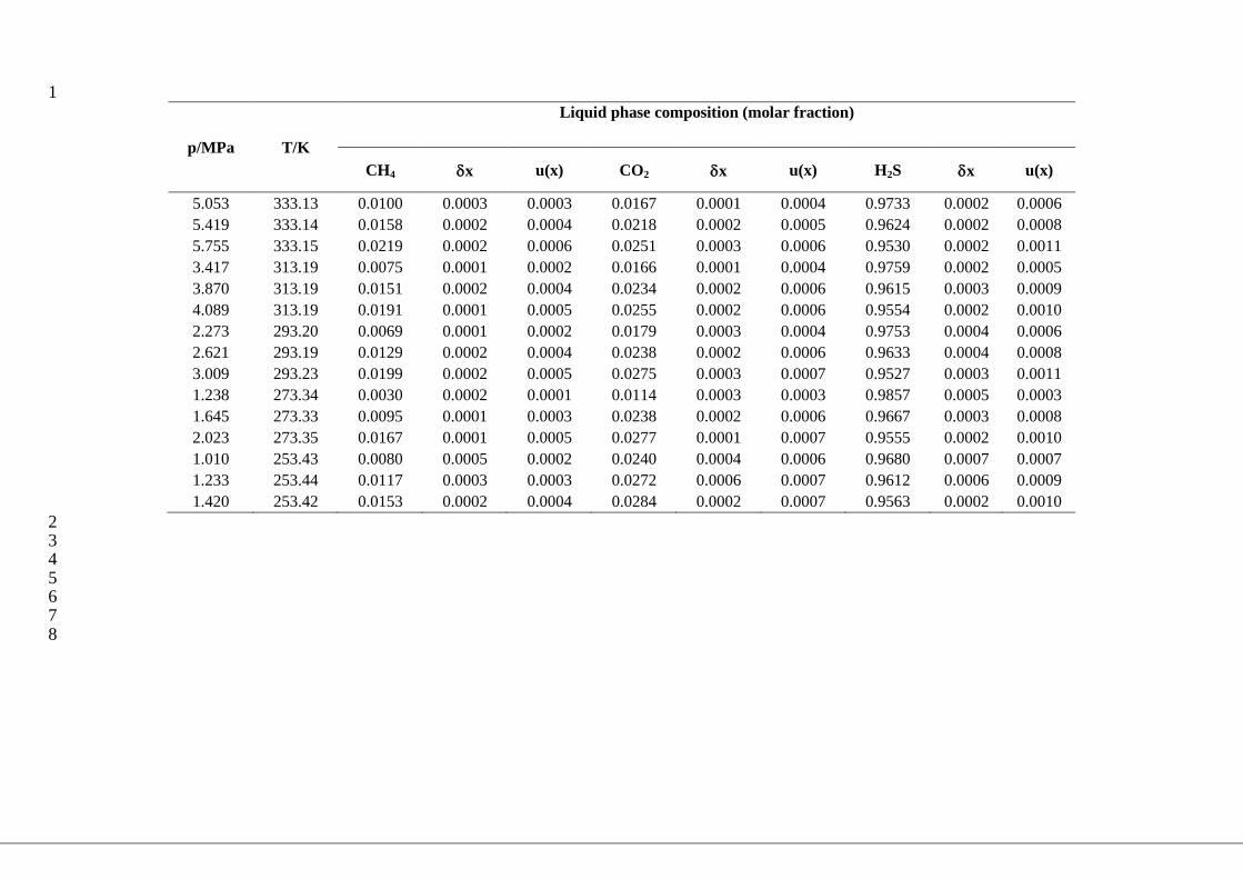
1

p/MPa T/K

Liquid phase composition (molar fraction)

CH4 x u(x) CO2 x u(x) H2S x u(x)

5.053 333.13 0.0100 0.0003 0.0003 0.0167 0.0001 0.0004 0.9733 0.0002 0.0006

5.419 333.14 0.0158 0.0002 0.0004 0.0218 0.0002 0.0005 0.9624 0.0002 0.0008

5.755 333.15 0.0219 0.0002 0.0006 0.0251 0.0003 0.0006 0.9530 0.0002 0.0011

3.417 313.19 0.0075 0.0001 0.0002 0.0166 0.0001 0.0004 0.9759 0.0002 0.0005

3.870 313.19 0.0151 0.0002 0.0004 0.0234 0.0002 0.0006 0.9615 0.0003 0.0009

4.089 313.19 0.0191 0.0001 0.0005 0.0255 0.0002 0.0006 0.9554 0.0002 0.0010

2.273 293.20 0.0069 0.0001 0.0002 0.0179 0.0003 0.0004 0.9753 0.0004 0.0006

2.621 293.19 0.0129 0.0002 0.0004 0.0238 0.0002 0.0006 0.9633 0.0004 0.0008

3.009 293.23 0.0199 0.0002 0.0005 0.0275 0.0003 0.0007 0.9527 0.0003 0.0011

1.238 273.34 0.0030 0.0002 0.0001 0.0114 0.0003 0.0003 0.9857 0.0005 0.0003

1.645 273.33 0.0095 0.0001 0.0003 0.0238 0.0002 0.0006 0.9667 0.0003 0.0008

2.023 273.35 0.0167 0.0001 0.0005 0.0277 0.0001 0.0007 0.9555 0.0002 0.0010

1.010 253.43 0.0080 0.0005 0.0002 0.0240 0.0004 0.0006 0.9680 0.0007 0.0007

1.233 253.44 0.0117 0.0003 0.0003 0.0272 0.0006 0.0007 0.9612 0.0006 0.0009

1.420 253.42 0.0153 0.0002 0.0004 0.0284 0.0002 0.0007 0.9563 0.0002 0.0010

2 3 4 5 6 7

8

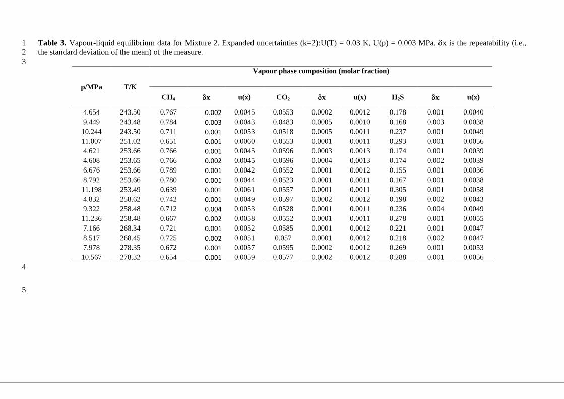
Table 3. Vapour-liquid equilibrium data for Mixture 2. Expanded uncertainties (k=2):U(T) = 0.03 K, U(p) = 0.003 MPa. x is the repeatability (i.e., 1

the standard deviation of the mean) of the measure. 2

3

p/MPa T/K

Vapour phase composition (molar fraction)

CH4 x u(x) CO2 x u(x) H2S x u(x)

4.654 243.50 0.767 0.002 0.0045 0.0553 0.0002 0.0012 0.178 0.001 0.0040

9.449 243.48 0.784 0.003 0.0043 0.0483 0.0005 0.0010 0.168 0.003 0.0038

10.244 243.50 0.711 0.001 0.0053 0.0518 0.0005 0.0011 0.237 0.001 0.0049

11.007 251.02 0.651 0.001 0.0060 0.0553 0.0001 0.0011 0.293 0.001 0.0056

4.621 253.66 0.766 0.001 0.0045 0.0596 0.0003 0.0013 0.174 0.001 0.0039

4.608 253.65 0.766 0.002 0.0045 0.0596 0.0004 0.0013 0.174 0.002 0.0039

6.676 253.66 0.789 0.001 0.0042 0.0552 0.0001 0.0012 0.155 0.001 0.0036

8.792 253.66 0.780 0.001 0.0044 0.0523 0.0001 0.0011 0.167 0.001 0.0038

11.198 253.49 0.639 0.001 0.0061 0.0557 0.0001 0.0011 0.305 0.001 0.0058

4.832 258.62 0.742 0.001 0.0049 0.0597 0.0002 0.0012 0.198 0.002 0.0043

9.322 258.48 0.712 0.004 0.0053 0.0528 0.0001 0.0011 0.236 0.004 0.0049

11.236 258.48 0.667 0.002 0.0058 0.0552 0.0001 0.0011 0.278 0.001 0.0055

7.166 268.34 0.721 0.001 0.0052 0.0585 0.0001 0.0012 0.221 0.001 0.0047

8.517 268.45 0.725 0.002 0.0051 0.057 0.0001 0.0012 0.218 0.002 0.0047

7.978 278.35 0.672 0.001 0.0057 0.0595 0.0002 0.0012 0.269 0.001 0.0053

10.567 278.32 0.654 0.001 0.0059 0.0577 0.0002 0.0012 0.288 0.001 0.0056

4

5

1

p/MPa T/K

Liquid phase composition (molar fraction)

CH4 x u(x) CO2 x u(x) H2S x u(x)

4.654 243.50 0.104 0.001 0.0025 0.0628 0.0002 0.0014 0.833 0.001 0.0034

9.449 243.48 0.331 0.005 0.0060 0.0662 0.0002 0.0013 0.603 0.005 0.0063

10.244 243.50 0.423 0.002 0.0066 0.0617 0.0007 0.0012 0.516 0.002 0.0067

11.007 251.02 0.499 0.002 0.0067 0.0600 0.0001 0.0012 0.441 0.002 0.0066

4.621 253.66 0.0896 0.0009 0.0022 0.0536 0.0004 0.0012 0.857 0.001 0.0030

4.608 253.65 0.090 0.001 0.0023 0.0537 0.0002 0.0012 0.857 0.001 0.0030

6.676 253.66 0.157 0.001 0.0036 0.0645 0.0002 0.0014 0.779 0.001 0.0043

8.792 253.66 0.251 0.002 0.0051 0.0675 0.0001 0.0014 0.681 0.002 0.0056

11.198 253.49 0.514 0.002 0.0067 0.0596 0.0001 0.0012 0.427 0.002 0.0066

4.832 258.62 0.0926 0.0006 0.0023 0.0509 0.0001 0.0011 0.8565 0.0006 0.0030

9.322 258.48 0.271 0.003 0.0054 0.0636 0.0003 0.0013 0.666 0.003 0.0058

11.236 258.48 0.445 0.004 0.0066 0.0614 0.0001 0.0012 0.493 0.004 0.0067

7.166 268.34 0.155 0.001 0.0036 0.0569 0.0001 0.0012 0.788 0.001 0.0042

8.517 268.45 0.211 0.002 0.0045 0.0610 0.0001 0.0013 0.728 0.002 0.0051

7.978 278.35 0.166 0.001 0.0038 0.0540 0.0001 0.0012 0.780 0.001 0.0043

10.567 278.32 0.282 0.001 0.0055 0.0598 0.0001 0.0012 0.659 0.001 0.0059

2

3

4

5

21

1

Table 4. Pure compound properties according to the Dortmund Data Bank and the Mathias-2

Copeman parameters from Reid et al.41

3

Formula CAS

number

Tc/K pc/MPa C1 C2 C3

CH4 74-82-8 190.60 4.600 0.0115 0.4157 -0.1727 0.3484

CO2 124-38-9 304.20 7.377 0.2236 0.7046 -0.3149 1.891

H2S 7783-06-4 373.55 8.937 0.1000 0.5077 0.0076 0.3423

4

22

Table 5. Vapor-liquid equilibrium pressures and phase compositions for the CH4 (1)-CO2 (2)-H2S (3) mixtures. Comparison between the experimental 1

and calculated data determined with the PR EoS and WS mixing rules. 2

T/K pexp/MPa x1 exp x2 exp y1 exp y2 exp y3 exp pcal/MPa y1 cal y2 cal y3 cal

243.50 4.654 0.104 0.0628 0.767 0.0553 0.1777 4.533 0.8125 0.0575 0.13

243.48 9.449 0.334 0.0662 0.794 0.0483 0.1577 9.301 0.7937 0.0483 0.158

243.50 10.244 0.423 0.0617 0.711 0.0518 0.2372 10.224 0.7353 0.0503 0.2145

258.62 4.832 0.0926 0.0509 0.742 0.0597 0.1983 4.784 0.7384 0.0614 0.2001

258.48 9.322 0.271 0.0636 0.712 0.0528 0.2352 9.513 0.7519 0.0537 0.1944

258.48 11.236 0.445 0.0614 0.667 0.0552 0.2778 11.683 0.6534 0.056 0.2906

268.34 7.166 0.155 0.0569 0.721 0.0585 0.2205 7.301 0.7172 0.0603 0.2225

268.45 8.517 0.211 0.061 0.725 0.057 0.218 8.837 0.7166 0.0588 0.2246

253.49 11.198 0.514 0.0596 0.639 0.0557 0.3053 11.619 0.6162 0.0566 0.3272

251.02 11.007 0.499 0.06 0.651 0.0553 0.2937 11.355 0.6402 0.0557 0.3042

253.66 4.621 0.09 0.0536 0.766 0.0596 0.1744 4.489 0.7595 0.0616 0.1789

253.65 4.608 0.09 0.0537 0.766 0.0596 0.1744 4.489 0.7594 0.0617 0.1789

253.66 6.676 0.157 0.0645 0.789 0.0552 0.1558 6.578 0.7853 0.0573 0.1574

253.66 8.792 0.251 0.0675 0.78 0.0523 0.1677 8.766 0.778 0.054 0.1679

278.35 7.978 0.166 0.054 0.672 0.0595 0.2685 8.154 0.6663 0.061 0.2727

278.32 10.567 0.282 0.0598 0.654 0.0577 0.2883 10.965 0.6449 0.0592 0.2959

333.13 5.053 0.01 0.0167 0.0698 0.0442 0.886 5.06 0.0656 0.0418 0.8927

333.14 5.419 0.0158 0.0218 0.1035 0.0538 0.8427 5.401 0.0948 0.0512 0.854

333.15 5.755 0.0219 0.0251 0.1335 0.0588 0.8077 5.726 0.1215 0.0558 0.8227

313.19 3.417 0.0075 0.0166 0.0885 0.0526 0.8589 3.43 0.0868 0.0529 0.8603

313.19 3.870 0.0151 0.0234 0.1522 0.066 0.7818 3.884 0.1507 0.0663 0.7829

313.19 4.089 0.0191 0.0255 0.1802 0.0689 0.7509 4.102 0.1787 0.0688 0.7525

293.20 2.273 0.0069 0.0179 0.1312 0.0677 0.8011 2.292 0.1318 0.0682 0.7999

293.19 2.621 0.0129 0.0238 0.2081 0.0785 0.7134 2.645 0.2101 0.0792 0.7107

293.23 3.009 0.0199 0.0275 0.2789 0.0796 0.6415 3.025 0.2792 0.0809 0.6399

273.34 1.238 0.003 0.0114 0.0953 0.0595 0.8452 1.263 0.1105 0.0588 0.8307

273.33 1.645 0.0095 0.0238 0.2547 0.0905 0.6548 1.664 0.2586 0.093 0.6483

273.35 2.023 0.0167 0.0277 0.3581 0.0889 0.553 2.042 0.3652 0.0894 0.5453

253.43 1.010 0.008 0.024 0.3405 0.1027 0.5568 1.038 0.3493 0.1026 0.5481

253.44 1.233 0.0117 0.0272 0.4334 0.0958 0.4708 1.225 0.4286 0.099 0.4724

253.42 1.420 0.0153 0.0284 0.493 0.089 0.418 1.398 0.4881 0.0913 0.4206 1

24

Table 6a. Values of the NRTL binary interaction parameters. 1

ij/J.mol-1

CH4 CO2 H2S

CH4 - 89 1119

CO2 3117 - 1140

H2S 2504 1904 -

2

3

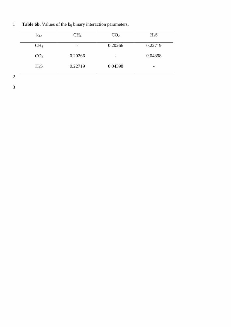
Table 6b. Values of the kij binary interaction parameters. 1

k12 CH4 CO2 H2S

CH4 - 0.20266 0.22719

CO2 0.20266 - 0.04398

H2S 0.22719 0.04398 -

2

3

26

Table 7. Vapor-liquid equilibrium pressures and phase compositions for the CH4 (1)-CO2 (2)-H2S (3) mixture (data from Ng et al.). Comparison 1

between the experimental and calculated data determined with the PR EoS and WS mixing rules. 2

T/K pexp/MPa x1 exp x2 exp y1 exp y2 exp pcal/MPa y1 cal y2 cal

199.15 1.499 0.0431 0.1313 0.9002 0.0648 1.2418 0.8881 0.0693

199.15 2.865 0.0971 0.1488 0.9317 0.0430 2.2399 0.9263 0.0459

199.15 4.195 0.1893 0.1424 0.9410 0.0338 3.3499 0.9428 0.0336

199.15 0.925 0.0357 0.3879 0.8015 0.1584 0.8838 0.7874 0.1648

199.15 2.838 0.1515 0.3129 0.9144 0.0628 2.4423 0.9118 0.0649

199.48 2.388 0.1314 0.4128 0.8761 0.0901 2.1325 0.8932 0.0832

199.54 3.519 0.2691 0.3652 0.8980 0.0700 3.0566 0.9168 0.0638

199.65 4.145 0.4283 0.2482 0.9260 0.0508 3.7214 0.9312 0.0483

204.65 2.703 0.1531 0.6609 0.8620 0.1228 2.5016 0.8590 0.1244

204.85 3.965 0.3301 0.5411 0.8885 0.0992 3.5680 0.8857 0.1019

206.15 1.378 0.0576 0.7156 0.7554 0.2126 1.3937 0.7628 0.2078

215.65 2.511 0.0734 0.1756 0.8515 0.0941 2.2607 0.8438 0.0956

215.65 4.573 0.2100 0.2453 0.8774 0.0810 4.0491 0.8782 0.0789

216.15 6.142 0.6272 0.1639 0.8732 0.0745 5.9673 0.8834 0.0693

226.76 5.668 0.3140 0.3217 0.8141 0.1258 5.3697 0.8223 0.1223

226.87 4.109 0.1677 0.3692 0.7817 0.1515 3.8890 0.7926 0.1479

226.95 5.506 0.3336 0.5327 0.7824 0.1880 5.2972 0.7824 0.1895

227.15 1.731 0.0408 0.2841 0.6593 0.2353 1.6771 0.6468 0.2390

227.45 7.777 0.2941 0.1020 0.8218 0.0645 6.7682 0.8694 0.0505

227.55 2.827 0.0626 0.1080 0.8226 0.0867 2.5006 0.8099 0.0918

227.55 4.864 0.1404 0.1273 0.8622 0.0674 4.3530 0.8572 0.0698

232.98 4.486 0.1346 0.1619 0.8165 0.0978 4.3312 0.8176 0.0962

233.04 5.852 0.2147 0.1902 0.8237 0.0968 5.5287 0.8243 0.0953

233.15 6.950 0.3095 0.1940 0.8135 0.0982 6.5007 0.8233 0.0940

254.85 6.171 0.1864 0.3198 0.6506 0.2163 6.0146 0.6521 0.2149

254.95 6.812 0.1641 0.1076 0.7563 0.0882 6.4674 0.7527 0.0901

254.95 9.060 0.2583 0.1076 0.7412 0.0847 8.4115 0.7532 0.0822

254.95 5.528 0.1687 0.6229 0.5472 0.3754 5.5495 0.5490 0.3750

255.05 6.895 0.2639 0.5708 0.5785 0.3505 6.9030 0.5797 0.3512

255.05 8.122 0.3784 0.4930 0.5699 0.3553 8.0494 0.5768 0.3513

255.15 3.513 0.0569 0.0769 0.6808 0.1071 3.2378 0.6699 0.1100

255.15 3.524 0.0645 0.2388 0.5622 0.2505 3.4060 0.5593 0.2516

255.15 8.501 0.3637 0.2939 0.6539 0.2054 8.2855 0.6574 0.2027

277.15 7.681 0.1792 0.2746 0.5213 0.2499 7.5311 0.5212 0.2480

277.25 9.515 0.2764 0.2861 0.5156 0.2503 9.1125 0.5155 0.2486

282.15 5.948 0.0885 0.0827 0.5804 0.1034 5.5900 0.5588 0.1187

282.65 10.549 0.2677 0.0985 0.5959 0.0958 10.4510 0.5984 0.0976

283.15 8.239 0.1632 0.0897 0.6102 0.0996 8.0840 0.6065 0.1013

285.40 11.838 0.3585 0.0983 0.5066 0.0980 11.8980 0.5376 0.0969

1

2

28

Table 8. Group interaction parameters3,43,44

(Akl = Alk)/MPa and (Bkl = Blk)/MPa needed to apply 1

the PPR78 model. 2

CH4 (group 5) CO2 (group 12) H2S (group 14)

CH4 (group 5) 0

CO2 (group 12) A12-5 = 136.57

B12-5 = 214.81 0

H2S (group 14) A14-5 = 190.10

B14-5 = 307.46

A14-12 = 135.20

B14-12 = 199.02 0

3

4

29

Figure 1. Relative deviations between the calculated (with the PR EoS and WS mixing rules) and 1

experimental bubble pressure and vapour phase composition. These data were measured in this 2

study. 3

4

-5

-4

-3

-2

-1

0

1

2

3

4

5

0 2 4 6 8 10 12

Rela

tive d

evia

tio

n /%

P exp /MPa

-10

-8

-6

-4

-2

0

2

4

6

8

10

0.0 0.2 0.4 0.6 0.8 1.0

Rela

tive d

evia

tio

n /%

y 1 exp

-6

-4

-2

0

2

4

6

0.00 0.02 0.04 0.06 0.08 0.10

Re

lati

ve

de

via

tio

n /%

y 2 exp

-10

-8

-6

-4

-2

0

2

4

6

8

10

0.0 0.2 0.4 0.6 0.8 1.0

Re

lati

ve

de

via

tio

n /%

y 3 exp

30

1

Figure 2. Relative deviations between the calculated (with the PR EoS and WS mixing rules) and 2

experimental bubble pressure and vapour phase composition. The data were obtained from Ng et 3

al., and the model parameters were adjusted based on the data acquired in this work ( 199 < T/K < 4

234, 254 < T/K < 286). 5

6

-5

0

5

10

15

20

25

0 2 4 6 8 10 12

Rela

tive d

evia

tio

n /%

P exp /MPa-10

-8

-6

-4

-2

0

2

4

6

0.4 0.5 0.6 0.7 0.8 0.9 1.0

Rela

tive d

evia

tio

n /%

y 1 exp

-20

-15

-10

-5

0

5

10

15

20

25

0.00 0.05 0.10 0.15 0.20 0.25 0.30 0.35 0.40

Re

lati

ve

de

via

tio

n /%

y 2 exp

-20

-15

-10

-5

0

5

10

15

20

0.00 0.10 0.20 0.30 0.40 0.50

Re

lati

ve d

evia

tio

n /%

y 3 exp

31

1

2

3

Figure 3. Relative deviations between the calculated (with the PPR78 model) and experimental 4

bubble pressure (a) and vapour phase composition (b-d) measured in this study. 5

6

0 6 12-10

0

10

20

30

40

50

Rel

ati

ve

dev

iati

on

/ %

P / MPa

(a)

0.0 0.5 1.0-30

-20

-10

0

10

20

30(b)

devy1

Rel

ati

ve

dev

iati

on

/ %

y1 exp

0.00 0.05 0.10-30

-20

-10

0

10

20

30(c)

devy2

Rel

ati

ve

dev

iati

on

/ %

y2 exp

0.0 0.5 1.0-50

0

50

100(d)

devy3

Rel

ati

ve

dev

iati

on

/ %

y3 exp

32

1

2

3

Figure 4. Relative deviations between the calculated (with the PPR78 model) and experimental 4

bubble pressure (a) and vapour phase composition (b-d). The data were obtained from Ng et al. 5

6

7

0 6 12

0

100

200

300

400

500

600

700

800

900

1000(a)

devP

Rel

ati

ve

dev

iati

on

%

P / MPa

0.0 0.5 1.0-50

0

50(b)

devy1

Rel

ati

ve

dev

iati

on

/ %

y1 exp

0.0 0.5 1.0-50

0

50

100(c)

devy2

Rel

ati

ve

dev

iati

on

/ %

y2 exp

0.0 0.5 1.0

0

100

200

300

400

500

600

700

800

900

1000(d)

devy3

Rel

ati

ve

dev

iati

on

%

y3 exp

33

1

2

180 220 260 300

0

5

10

15

DP (PPR78)

BP (PPR78)

2-liquid-phase boundary (PPR78)

3-phase boundary (PPR78)

2-phase boundary (exp)

3-phase boundary (exp)

critical points (exp)

Pre

ssure

/MPa

Temperature/K 3

Figure 5. PT phase envelope of the CH4 (1) + CO2 (2) + H2S (3) mixture (x1 = 0.4988, x2 = 0.0987, 4

x3 = 0.4022) as predicted by the PPR78 model. The experimental data (according to the symbols) 5

are those reported by Ng et al. DP = dew-point curve, BP = bubble-point curve. 6

7

34

1

Figure 6. PT phase envelope of the CH4 (1) + CO2 (2) + H2S (3) mixture (x1 = 0.4988, x2 = 0.0987, 2

x3 = 0.4022) as predicted with the PR EoS and WS mixing rules. The experimental data (according 3

to the symbols) are those reported by Ng et al. 4

5

0

5

10

15

180 200 220 240 260 280 300 320

Pre

ssu

re /

MP

a

Temperature /K

35

1

2

Figure 7. PT phase envelope of CH4 (1) + CO2 (2) + H2S (3) mixture 1 (x1 = 0.0406, x2 = 0.0311, 3

x3 = 0.9283) studied in this work. (a) Prediction with the PPR78 model. (b) Prediction with the PR 4

EoS and WS mixing rules (symbol: calculated critical point). DP = dew-point curve, BP = bubble-5

point curve. 6

7

180 280 3800

5

10

P /

MP

a

T / K

DP (PPR78)

BP (PPR78)0

1

2

3

4

5

6

7

8

9

10

180 200 220 240 260 280 300 320 340 360 380

Pre

ssu

re /

MP

a

Temperature /K

(a) (b)

36

1

2

Figure 8. PT phase envelope of CH4 (1) + CO2 (2) + H2S (3) mixture 2 (x1 = 0.5831, x2 = 0.0573, 3

x3 = 0.3596) studied in this work. (a) Prediction with the PPR78 model. (b) Prediction with the PR 4

EoS and WS mixing rules (symbol: calculated critical point). DP = dew-point curve. 5

6

180 220 260 3000

5

10

15

P /

MP

a

T / K

DP (PPR78)

3-phase boundary (PPR78)

0

2

4

6

8

10

12

14

16

18

20

180 200 220 240 260 280 300

Pre

ssu

re /

MP

a

Temperature /K

(a)

(b)

37

1

TOC Graphic 2

3

4

180 220 260 300

0

5

10

15

4

2

2

50% CH

10% CO

40% H S

two-liquid-phase

boundary

dew-point locus

Pre

ssure

/MPa

Temperature/K

bubble-point locus

Vapor-liquid critical point

Liquid-liquid

critical point

narrow 3-phase

region

5 6

7

8