
Vanderbilt University Department of Economics Working ...
37
Transcript of Vanderbilt University Department of Economics Working ...


Vanderbilt University Department of Economics Working Papers, VUECON-13-00007
Great Earthquakes, Exchange Rate Volatility and
Government Interventions�
Mariko Hatasey, Mototsugu Shintaniz and Tomoyoshi Yabux
This version: March 2013
Abstract
The Great East Japan Earthquake in 2011, as well as the Great Hanshin-Awaji
Earthquake in 1995 and the Great Kanto Earthquake in 1923, resulted in disorderly
movements of yen in the foreign exchange market. This paper investigates the exchange
rate volatility shift after these three great earthquakes in Japan and examines if similar
excess volatility after major earthquakes can also be observed in other countries. In
addition, using a unique daily data set from the Great Kanto Earthquake period, the
episode with the largest increased volatility among all three great earthquakes, we esti-
mate a reaction function of foreign exchange market intervention, and evaluate the role
of government intervention in stabilizing the foreign exchange market during the time
of increased uncertainty caused by a large unexpected negative shock in the economy.
Keywords: foreign exchange intervention; natural disasters; propensity score
JEL classi�cation: F31
�The authors thank Mario Crucini, Yanqin Fan, Takeshi Hoshikawa, Masanao Ito, Takatoshi Ito, YushiYoshida and seminar and conference participants at Bank of Japan, Board of Governors of the FederalReserve System, International Monetary Fund, Kyushu University, University of Tokyo, and Vanderbilt Uni-versity for their helpful comments and discussion. We also thank Akira Oseki, Shintaro Sugiyama andAyaka Ogura for their research assistance. Shintani gratefully acknowledges �nancial support through theNational Science Foundation Grant SES-1030164. The views expressed in this paper are those of the au-thors and do not necessarily re�ect the o¢ cial views of the Bank of Japan. Address correspondence to:Mototsugu Shintani, Department of Economics, Vanderbilt University, Nashville, TN 37235, USA; e-mail:[email protected].
yBank of JapanzDepartment of Economics, Vanderbilt UniversityxFaculty of Business and Commerce, Keio University

Vanderbilt University Department of Economics Working Papers, VUECON-13-00007
1 Introduction
On March 11, 2011, the eastern area of Japan was hit by a major earthquake followed
by tsunami, an event which resulted in an estimated capital stock losses of more than 210
billion US dollars. A week after this �Great East Japan Earthquake,� in response to the
resulting �excess volatility and disorderly movements�of the Japanese yen, the G-7 �nancial
authorities announced that they would jointly intervene the foreign exchange market for the
�rst time in ten years. While Japan is known for its very frequent earthquakes because of
its geographical location surrounded by plate boundaries, devastating major earthquakes of
this scale (magnitude) are considered rare events. In the past century, the two other major
earthquakes prior to this one were the �Great Kanto Earthquake,�which hit the Tokyo and
Yokohama areas in 1923, and the �Great Hanshin-Awaji Earthquake�which devastated the
city of Kobe and its surroundings in 1995. Since all three great earthquakes occurred in
populated areas, they had a larger negative impact on economic activities than any other
natural disasters in modern Japanese economic history.
From the economic point of view, earthquakes can be interpreted as unexpected negative
real shocks in the economy. Minor vibrations are frequently observed in Japan but they result
only in negligible economic losses. In contrast, rare but disastrous quakes can signi�cantly
change nation�s macroeconomic fundamentals, at least in the short-run. Because macroeco-
nomic fundamentals are re�ected in a nation�s currency value in the foreign exchange market,
we conjecture that increased uncertainty in fundamentals caused by major earthquakes in-
creases the instability of exchange rates under the �oating system. For example, the Japanese
yen depreciated rapidly after the Great Kanto Earthquake in 1923, while it appreciated after
both the Great Hanshin-Awaji Earthquake in 1995 and the Great East Japan Earthquake in
2011. In the past, the economic analysis of natural disasters has been conducted in various
contexts.1 However, to the best of our knowledge, there are no studies that focus on the e¤ect
1For example, there are studies on natural disasters with foci on economic growth (Skidmore and Toya,2002), national institutional quality (Kahn, 2005), international transfer (Strömberg , 2007) and consumption
1
Vanderbilt University Department of Economics Working Papers, VUECON-13-00007
of earthquakes or other natural disasters on the exchange rate volatility.
The objective of this paper is to empirically investigate the e¤ect of earthquakes on the
foreign exchange market and the role of subsequent government interventions, using historical
time series data. In particular, we �rst statistically examine whether there was increased
exchange rate volatility after the three great earthquakes in Japan. We show that, while the
directions of change di¤ered, all three great earthquakes were followed by a large exchange
rate �uctuations in the short-run. We further examine if similar increased exchange rate
volatility after earthquakes can be also observed in other countries under a �exible exchange
rate regime. In the second half of the analysis, we focus on the Great Kanto Earthquake, the
episode with the largest increased volatility among all three great earthquakes, and examine
if government intervention was e¤ective in stabilizing the foreign exchange market during the
time of increased uncertainty caused by a large unexpected negative shock in the economy.
By taking advantage of a unique data set from this period, we estimate a reaction function of
foreign exchange market intervention and �nd that the Japanese monetary authorities were
successful in stabilizing the exchange market.
Currency and �nancial crises, including the recent global �nancial crisis, are also well-
known for generating instability in both the currency and equity markets, and their empirical
characteristics have been extensively investigated using historical data by many studies in-
cluding Kaminsky and Reinhart (1998, 1999), Eichengreen (2008) and Reinhart and Rogo¤
(2008, 2009), among others. Major earthquakes are similar to currency crises in the sense that
they are negative shocks on economic activities that occur in much less often than in business
cycle frequencies.2 However, as argued in Kaminsky and Reinhart (1999), a currency crisis
is often preceded by problems in the banking sector, and several types of warning indicators
may be used to predict a future crisis. In contrast, the occurrence of earthquakes is impos-
sible to predict so that a direct comparison of subsamples of before and after earthquakes is
risk-sharing (Sawada and Shimizutani, 2008).2Using a representative consumer model, Barro (2009) shows that estimated welfare loss from rare disasters
can be as large as 20 percent of real GDP compared to 1.5 percent loss from normal business cycle �uctuations.
2

Vanderbilt University Department of Economics Working Papers, VUECON-13-00007
possible.3 This di¤erence distinguishes our analysis from other empirical studies of economic
crisis.
Our analysis is also closely related to the empirical literature on measuring the e¤ect of
foreign exchange market interventions (see Dominguez and Frankel, 1993, and Sarno and
Taylor, 2001, for extensive surveys). A widely accepted view of the goal of government
intervention is to stabilize the foreign exchange market.4 Empirical evidence of the role
of intervention in reducing the volatility of exchange rates is, however, rather mixed. For
example, Baillie and Osterberg (1997) and Dominguez (1998) use daily data of interventions
by US, German and Japanese central banks from the period around the Plaza and Louvre
agreements and �nd weak evidence on reducing volatility. Further mixed evidence on the
role of Japanese government intervention in reducing yen-dollar exchange rate volatility after
1990s is also reported by Chang and Taylor (1998), Nagayasu (2004), Watanabe and Harada
(2006) and Hoshikawa (2008).
There are at least three notable features in our analysis of exchange market interventions
that di¤er from the previous studies listed above. First, we use a newly constructed daily
data set of exchange rates and interventions for the period before and after the Great Kanto
Earthquake. This is the �rst formal empirical study on the e¤ect of exchange market in-
terventions in the 1920s. Second, unlike the previous analysis based on daily exchange rate
data, our estimation su¤ers less from an endogenous bias problem because the fact of a slower
decision-making process during 1920s has been con�rmed by historical documents. In con-
trast, in the analysis based on the recent data, the endogeneity of the intervention needs to
be incorporated by instrumental variables that are very di¢ cult to �nd in daily data. Third,
3The Japanese government passed the Large-Scale Eathquake Countermeasure Act in 1978 so that theJapan Meteorological Agency (JMA) can operate a real-time monitoring system to detect any warning signalsof major earthquakes. The system, however, failed to predict both the Great Hanshin-Awaji Earthquake in1995 and the Great East Japan Earthquake in 2011.
4For example, in the recent post-earthquake coordinated intervention on March 18, 2011, G-7 �nancialauthorities announced that: �As we have long stated, excess volatility and disorderly movements in exchangerates have adverse implications for economic and �nancial stability. We will monitor exchange markets closelyand will cooperate as appropriate.�
3

Vanderbilt University Department of Economics Working Papers, VUECON-13-00007
our data contains an o¢ cial government target exchange rate, which helps us to identify the
reaction function of monetary authorities. Because target rates are directly observed, there
is no need for making assumptions on how target rates are determined.5 We take advantage
of the reaction function estimate and employ the propensity score method to evaluate the
e¤ectiveness of intervention in reducing the exchange rate volatility. This estimation strat-
egy has been widely used to evaluate the average treatment e¤ect in the microeconometric
literature, but has recently attracted increasing attention in estimating the causal e¤ect of
policy variables using macroeconomic time-series, including Angrist and Kuersteiner (2011),
among others.
The rest of the paper is organized as follows. In section 2, statistical evidence of in-
creased volatility after major earthquakes is presented. Both historical results from three
great earthquakes in Japan and earthquakes from other countries are reported. In section 3,
using data from 1920s, we investigate the e¤ectiveness of market interventions in reducing
exchange rate volatility during a time of foreign exchange rate market instability caused by
a major earthquake. Concluding remarks are provided in section 4.
2 Exchange Rate Volatility and Earthquakes
2.1 Japanese evidence
We �rst investigate the behavior of the daily yen-dollar exchange rate during the periods
around three great earthquakes in Japan. Since earthquake occurrence cannot be predicted,
it is safe to say that an earthquake has no e¤ect on the exchange rates prior to the day of
the earthquake. Thus, we can simply split the sample at the date each earthquake occurred
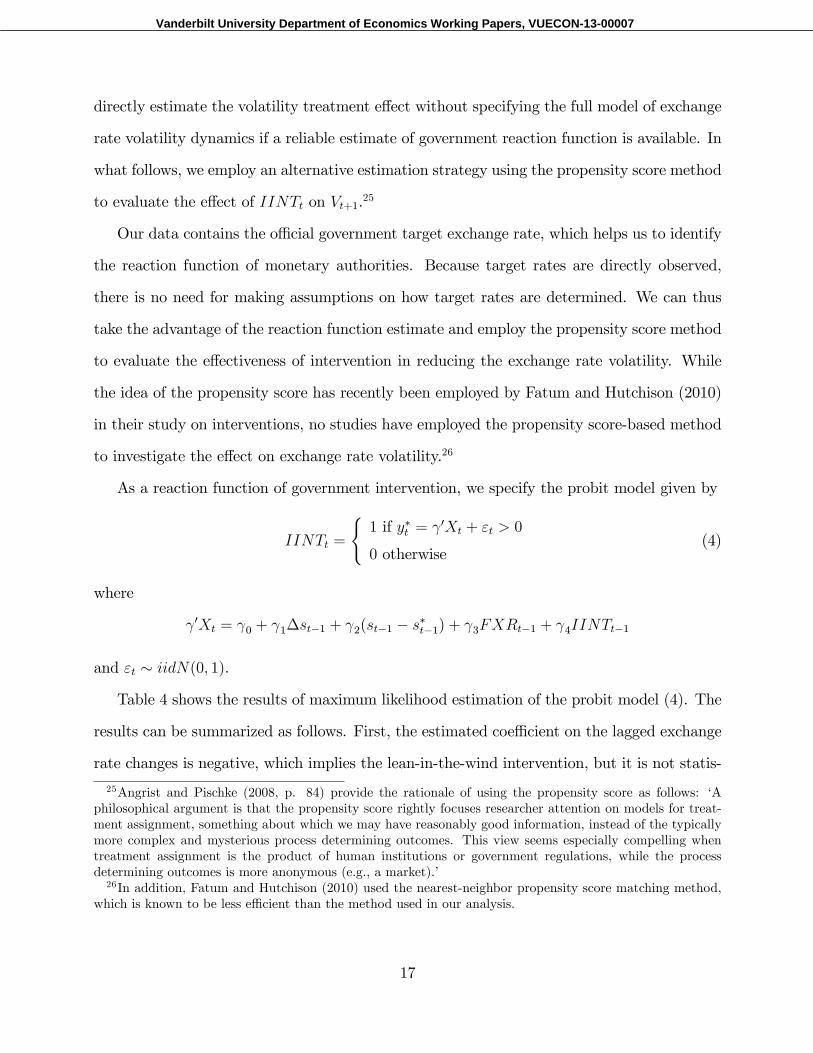
and compare the behavior of exchange rates between two subperiods.6 Figure 1 plots daily
5For example, Ito and Yabu (2007) assume that the target rate is determined as a function of past movingaverages of exchange rates.
6Splitting the sample is a more di¢ cult task in the analysis of �nancial or currency crisis. For example,a sudden depreciation of currency values in crisis is typically preceded by the overvaluation of the currency.Thus, to compare the empirical characteristics between the time of crisis and tranquil times, the latter is
4

Vanderbilt University Department of Economics Working Papers, VUECON-13-00007
yen-dollar exchange rate series from one year before the earthquake to one year after the
earthquake.
Panel A of the �gure shows yen-dollar exchange rates before and after the Great Kanto
Earthquake, which occurred on September 1, 1923.7 Prior to the earthquake, exchange rates
were relatively stable around 2 yen per US dollar. After the earthquake, however, the yen
depreciated dramatically and reached a level around 2.4 yen per US dollar during the �rst half
of the following year. This 20 percent depreciation of the yen may re�ect the market responses
to the deterioration of macroeconomic fundamentals. According to Sawada and Shimizutani
(2008), estimated housing property and capital stock losses from the Great Kanto Earthquake
was 32.6 billion US dollars in 2003 prices, which is equivalent to 43.6 percent of Japanese
GDP in 1923. In consequence, real GDP and export in 1923 dropped by 4.6 percent and by
10.3 percent, respectively, from the previous year.
Panel B of the �gure shows yen-dollar exchange rates before and after the Great Hanshin-
Awaji Earthquake, which occurred on January 17, 1995.8 Unlike the yen�s behavior after the
Great Kanto Earthquake, within three months, the yen appreciated in this instance for about
20 percent. Within a year, however, the exchange rate swung back to the pre-earthquake
level.
Panel C of the �gure shows yen-dollar exchange rates before and after the Great East
Japan Earthquake, which occurred on March 11, 2011. As in the case of the Great Hanshin-
Awaji Earthquake, the yen appreciated rapidly to 76.25 yen per dollar, which was at that
time the highest exchange rate recorded after World War II.
While the directions of change in the exchange rate di¤er, Figure 1 shows that all three
great earthquakes seem to cause increased exchange rate �uctuations.9 Let us turn to the
typically selected at 18 or 36 months prior to the crisis (see Kaminsky and Reinhart, 1998).7The exchange rate series is constructed from the New York Times (see Data Appendix).8The exchange rate series during this period as well as the period around the Great East Japan Earthquake
is obtained from Bloomberg.9A standard international real business cycle model predicts that an unexpected sudden reduction of
the capital stock causes the appreciation of real exchange rates. While we focus on nominal exchange rate�uctuations in this paper, we also examine (monthly) real exchange rates around three great earthquakes
5

Vanderbilt University Department of Economics Working Papers, VUECON-13-00007
issue of possible change in a volatility. In this paper, we employ two measures of volatility, the
absolute deviation and variance. Following the literature on the e¢ cient market hypothesis,
a white noise assumption is imposed on exchange rate growth, �st = st � st�1, where st
is the nominal yen-dollar exchange rate in logs. Since the mean exchange rate growth is
not signi�cantly di¤erent from zero, we here impose the zero drift condition and only report
uncentered �rst absolute sample moments and uncentered second moments.10 Table 1 shows
the descriptive statistics on the volatility before and after the earthquakes, using various
windows. The left panel of Table 1 shows the sample absolute deviation while the right panel
shows the sample variance. The sizes of the windows in computing the statistics are measured
in business days. On the whole, both measures show higher volatility after the earthquake
than before the earthquake. This result, however, somewhat varies depending on the choice of
windows. In the following analysis, we employ the 120-day-window pre-earthquake volatility
as a benchmark value of tranquil times to compare with the post-earthquake volatility. While
this choice of window is somewhat arbitrary, the good news is that the regime shift from the
tranquil period is unpredictable so that the e¤ect of earthquake is certainly excluded from
the pre-earthquake volatility measure.
For post-earthquake volatility, the window choice should depend on the timing of regime
shift from a turbulent regime to a tranquil regime. Unlike the abrupt transition at the time
of an earthquake, however, a gradual transition is expected from a turbulent regime to a
tranquil regime. Historical evidence from the Great Kanto Earthquake, which will later be
explained in detail, also suggests that the e¤ect of an earthquake on the economy persists for
at least one year. Because of these issues, we consider both 120 business days (approximately
six months) and 240 business days (approximately one year) as reasonable window sizes of the
post-earthquake volatility measures. If we compare the benchmark pre-earthquake volatility
and �nd that yen-dollar rates appreciated for all three episodes, consistent with the economic theory. Thisis due to increased wholesale prices in Tokyo area immediately after the Great Kanto Earthquake. However,for both real and nominal exchange rates, volatility is increased after the earthquakes.10Results are almost identical even if we replace uncentered sample moments with recentered (demeaned)
sample moments.
6

Vanderbilt University Department of Economics Working Papers, VUECON-13-00007
measure based on a 120-day-window and the post-earthquake volatility measures based on
120- and 240-day-windows, volatility is higher after the earthquake for all three events. In the
next section, we statistically test for regime shift in volatility as well as providing additional
international evidence.
Before we move on to further analysis, let us brie�y mention the frequency of govern-
ment intervention during these periods. When we use a 120-day-window before and after
the earthquake, the number of interventions increased from 12 to 29 during the period of
Great Kanto Earthquake. In case of the Great Hanshin-Awaji Earthquake, the frequency of
interventions increased from 19 to 36. In addition, coordinated interventions increased from
2 to 5. Finally for the Great East Japan Earthquake, the number increased from 0 to 2, and
the �rst involved coordinated interventions by G7. In section 3, we further investigate the
determinants and e¤ects of the intervention using the data from the period around the Great
Kanto Earthquake.
2.2 International evidence
We now extend our analysis of the previous section to international data to see if similar
increased volatility in the exchange rate can be commonly observed across countries. For an
obvious reason, we restrict our attention to the period after 1973 when the �oating exchange
system started among major countries. The EM-DAT is an international database on natural
disasters compiled by the Center for Research of the Epidemiology of Disasters (CRED).11
Among the natural disasters recorded in EM-DAT after 1973, we select countries and events
that satisfy the following three conditions: (i) natural disasters classi�ed as either earthquakes
or tsunamis; (ii) estimated loss from the disaster is above 5 percent of GDP; and (iii) the
exchange rate regime classi�ed by IMF is neither �xed nor pegged to other currencies within
�5 percent from the central rate.12 When we apply these criteria, 8 countries and 9 episodes11The data can be obtained from EM-DAT: The OFDA/CRED International Disaster Database (http:
www.emdat.be), Université Catholique de Louvain, Brussels, Belgium.12The classi�cation is based on IMF�s Annual Report on Exchange Arrangements and Exchange Restrictions.
7

Vanderbilt University Department of Economics Working Papers, VUECON-13-00007
are selected, and their daily exchange rate series from the period around the earthquakes are
obtained from Bloomberg.13 Note that earthquakes in Italy in 1980 and Greece in 1999 have
been selected in our sample since the currency bands of two countries were within �6 percent
and �15 percent, respectively, from the central rate. In contrast, the Sichuan earthquake
of 2008 in China is excluded because the IMF classi�ed China as a �crawling peg�around
the time of the earthquake. In addition, while the IMF�s classi�cation of Georgia was either
�independent �oating�or �managed �oating with no pre-annouced path for the exchange rate�
around the time of the earthquake in 2002, it is excluded from our sample since the daily
exchange rate data shows that rates did not change for more than 70 percent of the time.
Table 2A summarizes the results of international comparison including the three great
earthquakes in Japan. The �rst column shows the mean absolute deviation of tranquil time
based on a 120-day-window. The volatility of tranquil times varies across countries. The
smallest volatility is found in the pre-Great Kanto Earthquake period in Japan. The largest
volatility is found in Algeria. The second and third columns show the absolute deviation ratios
using post-earthquake period volatility based on 120-day- and 240-day-windows, respectively.
The ratio above one corresponds to the case of increased volatility after earthquakes. The
absolute deviation ratio is greater than one for 11 out of 12 events when a 120-day-window is
used for both before and after the earthquake. The ratios clearly show that the Great Kanto
Earthquake stands out in terms of the relative change in the volatility. When a 120-day-
window for the post earthquake period is replaced by a 240-day-window, somewhat weaker
evidence is obtained with the number of increased volatility reduced from 11 to 9. This indi-
cates that a gradual transition from a turbulent regime to a tranquil regime may be completed
between 6 months and 1 year in some countries. The fourth to sixth columns represent cor-
responding measures based on sample variance. Similar to the absolute deviation, increased
variance is observed in majority of the countries.
Let Vt be a realized volatility measure de�ned either by Vt = j�stj or Vt = (�st)2. To
13An exception is Turkey which is obtained from the Central Bank of Turkey.
8

Vanderbilt University Department of Economics Working Papers, VUECON-13-00007
conduct a formal test on whether the volatility is increased after the earthquake, we run the
following regression:
Vt = �0 + �1DEQt + ut (1)
where ut is a zero mean regression error term and DEQt is a dummy variable which takes
a value 1 after the earthquake and 0 before the earthquake. In regression analysis, we use
the same 120-day-window before and after the earthquake, which results in a sample of size
240. We report the heteroskedasticity- and autocorrelation-consistent (HAC) standard errors
to incorporate the possibility of serial correlation. We further extend the simple regression
analysis of the variance shift (Vt = (�st)2) to the time-varying conditional heteroskedasticity
with a variance shift by estimating a GARCH(1,1) model given by
�st =pht"t (2)
ht = !0 + !1DEQt + !2"2t�1 + !3ht�1
where !0 > 0, !0 + !1 > 0, !2 � 0, !3 � 0 and "t � iidN(0; 1).
Table 2B reports ordinary least squares (OLS) estimates of the regression model (1) and
maximum likelihood estimates of the GARCH model (2). Coe¢ cients on earthquake dum-
mies in two volatility regressions are signi�cantly positive for the Great Kanto Earthquake
and the Great Hanshin-Awaji Earthquake, and are positive but not signi�cant for the Great
East Japan Earthquake. In the GARCH model, coe¢ cients on earthquake dummies are
signi�cantly positive for all three Japanese great earthquakes. In the case of Italy, all the co-
e¢ cients from volatility regressions and GARCH estimation are signi�cantly positive. In the
case of both Taiwan and Algeria, estimates from GARCH model are positive and signi�cant.
For Sri Lanka, �1�s are signi�cantly positive for two volatility dummy regressions but not for
the GARCH estimate. If we consider testing the null hypothesis of �1 � 0 or !1 � 0 against
the alternative of �1 < 0 or !1 < 0, the null cannot be rejected for all cases at the 5 percent
level. Thus, on the whole, statistical evidence seems to support our conjecture of increasing
9
Vanderbilt University Department of Economics Working Papers, VUECON-13-00007
volatility after major earthquakes.
3 Post-Earthquake Foreign Exchange Market Interven-
tions: A Case Study
3.1 Data and historical background
Prior to WWI, Japan held foreign exchange reserves as well as gold. During the 1920s,
as Japan recorded persistent current account de�cits, the yen tended to be under strong
downward pressures.14 The monetary authorities used intervention to curb �uctuations of
the yen. The government and the Bank of Japan (hereafter BOJ) started selling their foreign
currency denominated assets to private banks in early 1919 (Saito, 1982). Previous studies
reveal that, in the 1920s, sales were initially conducted to �nance imports and then the
purpose shifted into a¤ecting the level of foreign exchange rates.15
The foreign exchange markets during the 1920s developed in terms of both the volume
and technology.16 London was the leading market and New York followed (Cassis, 2006).17
The market participants were exchange brokers, dealers and for long term bills transactions,
large commercial �rms were active players as well. Japanese and other foreign banks fell
in one of the important categories of dealers (Madden and Nadler, 1935). The practice of
14The yen at the time was �oating as Japan was temporarily o¤ the gold standard system. For details, seethe Historical Appendix.15Saito (1982) states that the object of the sales evolved into supporting yen exchange rates in October
1921 when the government directed the Yokohama Specie Bank to keep its quotation rates at 48 dollarsper a hundred yen and sold foreign exchanges to it at the same time. Ito (1989) states that sales becamepolicy tools to support exchange rates in September 1922 when the �nance minister Ichiki explicitly showedthe intention of conducting foreign exchange sales for the purpose of absorbing the negative e¤ects of goldembargo on foreign exchange rates.16The �generalized �oating�with more opportunities for speculations led to an increase in trading volume
in major trading centers, and the trading practices and technology were developed during this �boom�period.Before WWI, the brokers met bi-weekly at the Royal Exchange in London. In the post-WWI period, thetrading through telephone or telegrams became more common in major markets (Takahashi, 2009; Evitt,1931).17Currencies of European countries, Canada, Mexico, China, India, the Philippine Islands, Java, Japan,
Straits Settlement and South American countries were actively traded in the New York market (Madden andNadler, 1935).
10
Vanderbilt University Department of Economics Working Papers, VUECON-13-00007
recording and publishing foreign exchange rates was prevalent in major trading centers by
the late nineteenth century (Flandreau and Jobst, 2005). In some markets, such as London
and New York, newspapers and magazines were the primary media for publication. Market
rates in these media were the prices quoted by dealers and were collected by each paper or
magazine (Evitt, 1931).
Considering the circumstances described above, we construct a daily series below for the
purpose of investigating the e¤ects of foreign exchange interventions around the time of the
Great Kanto Earthquakes (for details, see the Data Appendix). First, two series of daily data
sets for foreign exchange rates are constructed: yen exchange rates against the US dollar in
the New York market; and o¢ cial quotations of yen/dollar. It is likely that the latter refers
to �o¢ cial quotations by the Yokohama Specie Bank (Shokin Tatene),�which were supposed
to be rates o¤ered by the Yokohama Specie Bank (YSB) to its customers. However, they were
considered as a kind of policy target by the government and quoted rates often diverged from
actual trading rates.18 Figure 2 shows the development of market yen-dollar exchange rates
and target rates (o¢ cial quotations by the YSB). The value of the yen against the US dollar
peaked out in October 1922. The Great Kanto Earthquake occurred in September 1923 and
its aftermath brought the depreciation of the yen rate to the level around 2.22 yen per dollar
at the end of 1923 and then to 2.60 yen next year end.19 The year of 1925 saw the reverse of
this yen-depreciating trend. In the regression analysis, we denote this target rate in logs by
s�t .
Second, data series for sales and purchases of foreign exchanges by the BOJ or by the
18For example, the YSB was instructed by the monetary authorities to keep its quotation at the level of48 dollars per hundred yen in 1921 even though market rates fell below this line (Saito, 1982). The YSB hada mixed ownership, with the government holding a third of YSB�s capital when it was established in 1880.The bank�s primary role was to provide trade �nance, and it played a large part in Japan�s foreign exchangepolicies. It held reserves for o¢ cial bodies as overseas agencies for the BOJ during the interwar period.19The trade balance after the earthquake created a depreciating pressure on yen rates. The earthquake
caused the sharp decline in exports as the City of Yokohama, which was heavily hit by the disaster, was thecentre of raw silk exports. Stocks for exports there were lost owing to �re and the loss amount was equivalentas one tenth of raw silk exports in previous year. In the meantime, reconstruction materials were imported,leading to increase in imports (Bank of Japan Research Department, 1933; Shikata, 1926).
11

Vanderbilt University Department of Economics Working Papers, VUECON-13-00007
government through the BOJ are constructed from BOJ accounting books. Every single
transaction by the BOJ, including those on behalf of the government regarding the sales of
foreign currencies to private banks, is recorded in ledgers, and thus, the details of interventions
such as dates, amounts and counterparties are available. Figure 3 shows the amounts of
intervention. The dollar-selling interventions were conducted 60 times between April 1922
and September 1925, with the total amounts of 208 million dollars. There was only one
example of the dollar-purchasing intervention on September 4 1924, and it was for the amount
of 21 million dollars. Since one observation is not su¢ cient in statistical analysis, we focus
on the dollar-selling interventions in the following section and use an intervention dummy
variable, IINTt, that takes a value one for such an intervention.
Third, the data series for outstanding foreign exchange reserves on a daily basis are
constructed from the archival documents of the BOJ. Figure 4 shows the outstanding foreign
exchange reserves, which will be denoted by FXRt in the subsequent analysis. It follows
declining trends in the 1920s, re�ecting a series of interventions under the persistent current
account de�cits. In the mid 1920s, the government shifted its major policy tools for controlling
foreign exchange rates from intervention to gold shipments.20
3.2 Volatility regression and government intervention
The daily exchange rate data shows a large amount of increased volatility after the Great
Kanto Earthquake. At the same time, we observe that frequency of intervention increased
after the earthquake. Since we are interested in knowing the interaction between increased
volatility caused by the earthquake and government intervention, we focus on the e¤ectiveness
of intervention in terms of reducing the volatility of the exchange rate.
Theoretically, intervention can have an e¤ect on the level of exchange rates, the volatility
20The Ministry of Finance issued the statement on September 16, 1926 entitled �The Statement on theDomestic Specie Shipments,�declaring that �the government has decided to ship its domestic specie abroadif necessary. The �rst shipment will be carried out on the 20th of this month with four million dollars.�(Materials on Japanese Monetary History, vol. 21, p.391, authors�translation).
12

Vanderbilt University Department of Economics Working Papers, VUECON-13-00007
of exchange rates or both the level and volatility at the same time. The e¤ectiveness of
intervention is typically justi�ed either through the portfolio channel or signaling channel.
Dominguez (1998) emphasizes the signaling channel and discusses the possibility of reduc-
ing the volatility without changing the level of exchange rate if intervention signals are fully
credible and unambiguous and if the market is e¢ cient.21 She uses daily data on G-3 central
bank interventions from the 1977-1994 period and �nds that only overt interventions in the
mid-1980s reduced volatility, but not overt interventions in other periods and secret interven-
tions. In our analysis, we assume a simple random walk process for the exchange rate but
consider the role of government intervention in stabilizing the foreign exchange market by
estimating the variance structure of the random walk innovation.
In the evaluation of the e¤ectiveness of interventions based on the recent data, the en-
dogeneity of interventions needs to be incorporated either by using instrumental variables or
specifying the full model. However, �nding instrumental variables, which are correlated with
the exchange rate but uncorrelated with the error term, is an extremely di¢ cult task in the
context of daily observations.
In contrast, unlike the previous analysis based on daily exchange rate data, our estimation
su¤ers less from an endogenous bias problem because of the slower decision-making process
that characterizes the 1920s. The typical decision making process for intervention is as
follows. The government sets a policy of conducting sales operations in the foreign exchange
market, which is often announced by high government o¢ cials.22 Each private bank engaged
in foreign exchange business requests the BOJ to sell its o¢ cially held foreign currencies, with
the reason being its future shortage of foreign currencies. The bank in question, the BOJ
and the Ministry of Finance (MOF) go through the negotiation process about the amounts
21In particular, Dominguez (1998, p. 167) states that �if the information being signalled via interventionis that the central bank is comitted to reducing volatility (potentially the Louvre Accord interventions), thenwe should expect intervention to be associated with no systematic e¤ect on the level of the exchange rate andwith lower exchange rate variances.�22For example, the Finance Minister Ichiki stated �considering the negative e¤ect of the gold embargo
on foreign exchange rates, we adopt this policy to enable us to sell foreign exchange reserves in future�onSeptember 16, 1922 (Materials on Japanese Monetary History, vol. 21, p. 389, authors�translation).
13
Vanderbilt University Department of Economics Working Papers, VUECON-13-00007
of the sales and dates for transactions. When the negotiation is completed, the private bank
submits the formal request form to the BOJ, and the BOJ passes the request to the MOF.
The MOF then issues the permission for transactions. Usually the whole process took more
than one business day.23 In other words, within-day exchange rate movements cannot trigger
interventions on the same day.
Another important issue considered in the literature of exchange rate intervention is the
possibility of the regime shift. For example, Kearns and Rigobon (2005) proposed using
simulated GMM with the assumption of a known break date of intervention policy change.
Ito and Yabu (2004) also allow that parameters vary across regimes in Japan. Since, in the
previous section, we found a structural shift in volatility at the time of the earthquake, we
also consider the possibility that the e¤ect of intervention is regime-dependent.
As discussed in Section 2, the end of the post-earthquake period is not clearly de�ned
since a smooth transition from a turbulent regime to a tranquil regime is more likely than an
abrupt transition. For this reason, we check the robustness of the result by using two di¤erent
samples in which the end periods di¤er. Each end period is selected based on a notable policy
event that is likely to re�ect some change in the government�s view on economic conditions.
The �rst sample (labeled as Full sample 1) ends on September 16, 1925. This corresponds
to the date that main exchange rate policy instrument of Japanese monetary authorities
switched from interventions to gold shipments. The second sample (labeled as Full sample 2)
ends on April 15, 1925. This is the date when the BOJ lowered the o¢ cial interest rate. For
both cases, the sample starts on April 1, 1922 which is the earliest possible date available in
our data set.23As an example, the Daihyaku Bank submitted the formal request to the BOJ on July 18, 1923, asking
to provide 300,000 dollars on July 20. The letter from Daihyaku Bank to the BOJ dated on July 20 noti�edthat it paid the Japanese yen equivalent as the amount paid by the BOJ in dollars on that day. On the sameday, the BOJ sent a letter to the MOF, reporting that the dollar sales were conducted with Daihyaku Bank(source: Document 13266 in the data appendix). As another example, in the case of the dollar sales to theYSB settled on May 31, 1922, the record of the telephone conversation between the BOJ and the YSB revealsthat the negotiation had started before May 24 (source: Historical Materials 0076 in the data appendix).
14

Vanderbilt University Department of Economics Working Papers, VUECON-13-00007
The volatility model that we estimate has the following linear speci�cation:
Vt = �0 + �1DEQt + �2Vt�1
+�3IINTt + �4IINTt�1 + �5DEQt � IINTt + �6DEQt � IINTt�1 (3)
+�0Zt + ut
where Vt is either Vt = j�stj or Vt = (�st)2, IINTt is an indicator that takes value 1 on
days when there are dollar-selling (yen-purchasing) interventions and 0 otherwise, and Zt is
a vector of additional covariates. The earthquake dummy, DEQt, is an exogenous variable
and thus there is no endogeneity. The intervention dummy, IINTt, is typically treated as an
endogenous variable but for the reason explained in the previous section, the OLS estimation
remains valid. The lagged Vt is also included to allow for the possibility of GARCH e¤ects
when the variance measure is used.
Tables 3A and 3B show the results of the estimation based on the absolute deviation
and variance, respectively, using both Full sample 1 and Full sample 2. For additional co-
variates included in Zt, we consider lagged interest di¤erentials between Japan and the US
(RJAPANt�1�RUSt�1) and the lagged deviation of the spot exchange rate from the target
rate (st�1 � s�t�1). Estimated coe¢ cients on additional covariates are not reported in tables.
For other coe¢ cients, estimates are reported along with the HAC standard errors.
Let us �rst look at the coe¢ cient on the earthquake dummy, namely, �1. For both absolute
deviation and variance measures, �1�s in all the speci�cations are positive and signi�cant
at the 5 percent level. These results are consistent with our previous �nding of increased
volatility after the earthquake. For the absolute deviation, the estimated coe¢ cients �2�s
on the lagged volatility are positive and signi�cant. When variance is used, �2�s are also
positive and signi�cant unless additional covariates are included, implying some possibility
of GARCH structure.
We are mainly interested in coe¢ cients on the interaction term of the earthquake dummy
15

Vanderbilt University Department of Economics Working Papers, VUECON-13-00007
and the intervention dummy, namely, �5 and �6. When absolute deviation is used, �6 is
signi�cantly negative but �5 is not signi�cant for all the speci�cation. For the variance
measure, similar results are also obtained at a somewhat higher signi�cance level. This shows
that the intervention during the post-earthquake period is e¤ective in reducing one-period-
ahead volatility. In contrast, no instantaneous e¤ect of interventions on volatility is found
through our analysis. When we consider the market conditions at the time, the e¤ect of
intervention appearing on the next business day can be explained by the slow spread of
information in the market. Typically, only a counterparty of the transaction, say the YSB,
and monetary authorities knew about the intervention on the same day but not other market
participants.24
The remaining coe¢ cients �3 and �4 capture the e¤ect of intervention during the pre-
earthquake period. For all the cases, neither �3 nor �4 is signi�cant. This shows there is no
evidence supporting the role of intervention in reducing volatility during tranquil times.
In summary, our OLS estimates suggest that interventions reduce the exchange rate
volatility of the next business day during the period after the Great Kanto Earthquake.
In the next section, we use an alternative procedure to evaluate the e¤ect of intervention by
taking advantage of the target exchange rate series available in our data.
3.3 Policy propensity score and volatility treatment e¤ects
Using the OLS method, we �nd that an intervention operation today, represented by
IINTt, reduces the exchange rate volatility on the next business day, represented by Vt+1,
during the post-earthquake period. Because of the reason we stated before, our basic OLS
estimates of the e¤ect of intervention are not likely to su¤er from an endogeneity problem.
However, the validity of OLS estimates still relies on the assumption that the dynamic struc-
ture of exchange rate volatility is correctly described by equation (3). Alternatively, we can
24The details of the intervention often appeared in newspapers and other media that were not available onthe day of intervention.
16
Vanderbilt University Department of Economics Working Papers, VUECON-13-00007
directly estimate the volatility treatment e¤ect without specifying the full model of exchange
rate volatility dynamics if a reliable estimate of government reaction function is available. In
what follows, we employ an alternative estimation strategy using the propensity score method
to evaluate the e¤ect of IINTt on Vt+1.25
Our data contains the o¢ cial government target exchange rate, which helps us to identify
the reaction function of monetary authorities. Because target rates are directly observed,
there is no need for making assumptions on how target rates are determined. We can thus
take the advantage of the reaction function estimate and employ the propensity score method
to evaluate the e¤ectiveness of intervention in reducing the exchange rate volatility. While
the idea of the propensity score has recently been employed by Fatum and Hutchison (2010)
in their study on interventions, no studies have employed the propensity score-based method
to investigate the e¤ect on exchange rate volatility.26
As a reaction function of government intervention, we specify the probit model given by
IINTt =
(1 if y�t =
0Xt + "t > 0
0 otherwise(4)
where
0Xt = 0 + 1�st�1 + 2(st�1 � s�t�1) + 3FXRt�1 + 4IINTt�1
and "t � iidN(0; 1).
Table 4 shows the results of maximum likelihood estimation of the probit model (4). The
results can be summarized as follows. First, the estimated coe¢ cient on the lagged exchange
rate changes is negative, which implies the lean-in-the-wind intervention, but it is not statis-
25Angrist and Pischke (2008, p. 84) provide the rationale of using the propensity score as follows: �Aphilosophical argument is that the propensity score rightly focuses researcher attention on models for treat-ment assignment, something about which we may have reasonably good information, instead of the typicallymore complex and mysterious process determining outcomes. This view seems especially compelling whentreatment assignment is the product of human institutions or government regulations, while the processdetermining outcomes is more anonymous (e.g., a market).�26In addition, Fatum and Hutchison (2010) used the nearest-neighbor propensity score matching method,
which is known to be less e¢ cient than the method used in our analysis.
17

Vanderbilt University Department of Economics Working Papers, VUECON-13-00007
tically signi�cant. Second and most importantly, the coe¢ cient on the lagged deviation from
the target rate is positive and signi�cant. This outcome shows that if closing rate of yen in
the New York market is valued below the target rate, a yen-purchasing intervention is likely
to be conducted. Third, the coe¢ cient on the foreign exchange reserves is positive and sig-
ni�cant. When reserves decrease, the result shows that monetary authority is likely to avoid
the dollar-selling (yen-purchasing) intervention to prevent further decline in reserves. Finally,
the coe¢ cient on interventions on the previous business day is positive and signi�cant, thus
the intervention today is more likely to be followed by another intervention the next day.
Subsample estimates do not di¤er much from the full sample case except for the signif-
icance of some coe¢ cients. Before the earthquake, the coe¢ cient of the deviation from the
target is still positive but not signi�cant. For two subsample cases after the earthquake, the
sign of lagged intervention coe¢ cients is positive but not signi�cant. For other coe¢ cients,
the results are very similar to the full sample case. Overall, our probit estimation of the reac-
tion function is satisfactory, and thus we use the estimate to compute the policy propensity
score.
Following Angrist and Kuersteiner (2011), we employ the conditional independence as-
sumption (CIA) of the following form:
Vt+1 ? IINTtjXt
where ? denotes the independence, random variables to the right of the vertical bar are the
conditioning sets and Vt = j�stj or Vt = (�st)2. Combining the CIA with the probit model (4)
implies that, when Xt is given, the volatility does not depend on unobservable factors in the
determination of the intervention which are represented by "t in (4). We de�ne the volatility
treatment e¤ect by V TE = E[V1t+1 � V0t+1] where V1t+1 and V0t+1 are potential volatility
outcomes at time t+ 1 in case of an intervention and no intervention at time t, respectively.
In the case of Vt = (�st)2, the volatility treatment e¤ect corresponds to �21 � �20 where �21 is
18

Vanderbilt University Department of Economics Working Papers, VUECON-13-00007
the variance of the random walk innovation with intervention and �20 is the variance of the
random walk innovation without intervention.27 If an intervention has an e¤ect on reducing
the exchange rate volatility, we expect the volatility treatment e¤ect to be negative.
In what follows, we evaluate the volatility treatment e¤ect by using the inverse propensity
score weighting estimator given by
[V TE =TXt=1
(IINTt � bp(Xt))Vt+1bp(Xt) (1� bp(Xt))
where bp(Xt) is the estimated propensity score from equation (4). Under the CIA, this esti-
mator is known to be free of selection bias even if not all potential outcomes are observed.
We evaluate the precision of the estimate by reporting the 95 percent con�dence intervals
obtained from a block bootstrap method.28 For the purpose of comparison with our inverse
propensity score weighting estimator, we also report a simple estimator of volatility treatment
e¤ects using the regression adjustment based on the propensity score.29
Table 5 reports estimates of volatility treatment e¤ects using various subsamples. First,
for the full sample estimate, which ignores the e¤ect of earthquake, the treatment e¤ects are
negative but small both in terms of absolute deviation and variance. The con�dence interval
contains both positive and negative values. This result is likely to be the re�ection of mixing
both pre-earthquake and post-earthquake samples even if the intervention works di¤erently
in two regimes. The regression adjustment estimates are very close to the inverse probability
weighting estimate.
Second, for the pre-earthquake subsample, volatility treatment e¤ects turn out to be
positive. However, the con�dence interval contains the negative range as well. This result is
consistent with the OLS estimate in the previous subsection, and shows that intervention did
27A similar treatment e¤ect on variance has also been considered by Firpo (2010) in the context of a policye¤ect on cross-sectional income dispersion.28The block length in the bootstrap is set at �ve business days.29The regression adjustment is based on an auxiliary regression of the form: Vt+1 = �0 + �1IINTt +
�2bp(Xt) + ut+1 where �1 is the volatility treatment e¤ect. A symmetric con�dence interval from a naivestandard error is reported.
19

Vanderbilt University Department of Economics Working Papers, VUECON-13-00007
not contribute much in reducing the exchange rate volatility in the tranquil regime with low
volatility.
Third, for the post-earthquake subsample, negative volatility treatment e¤ects are ob-
tained with much less negative value than the full sample case. Thus, during the post-
earthquake period when volatility is high, intervention is e¤ective in reducing the volatility of
exchange rates. The con�dence intervals show that their upper bounds are still less negative
than the point estimate of the full sample case. This main �nding of our paper is robust even
if we change the measure of volatility from absolute deviation to variance, or use alternative
post-earthquake subsample periods. The regression adjustment method also provides results
similar to those from the inverse propensity score weighting method.
4 Conclusion
In the case of three great earthquake in Japan, we found evidence of increasing volatility
of exchange rates in the post-earthquake period compared to the pre-earthquake period.
For other countries su¤ering from earthquakes of similar magnitude in terms of economic
losses, we also found evidence of increased volatility. We conjecture that these observations
re�ect the fact that a devastating earthquake increases uncertainty about the nation�s future
economic fundamentals.
Using data from the Great Kanto Earthquake episode, where increased relative volatility
was highest among the three great earthquakes, we found that government intervention was
indeed e¤ective in reducing the volatility of exchange rates. We also note that the e¤ectiveness
of the intervention can only be found in the period of increased uncertainty caused by the
earthquake but not in the tranquil times preceding the earthquake.
20

Vanderbilt University Department of Economics Working Papers, VUECON-13-00007
Data Appendix
Data used in the analysis of exchange market interventions from the 1920s are constructed
from the following sources.
1. Yen exchange rates against the US dollar in the New York market (st): Closing rates in
the New York market applied to transactions through cables (source: New York Times).
2. O¢ cial quotations of yen/dollar (s�t ): It is likely that this series involves �o¢ cial quo-
tations by the Yokohama Specie Bank (Shokin Tatene),�judging from its development,
although no notes are available in the historical material from which the data are taken.
Figures after 1927 are identical as o¢ cial quotations by the YSB in Table II, History
of the Yokohama Specie Bank, vol. 6 (source: �Financial Summary Tables [Kinyu
Yoryaku], Bank of Japan Institute for Monetary and Economic Studies Archives, doc-
uments 14277-14291).
3. Sales of foreign exchanges by the BOJ or by the government through the BOJ (used to
construct IINTt): In ledgers, the dates of the settlements for intervention are recorded.
We assume the transaction dates are two business days prior based on the fact that
two business days routinely elapsed from the submission of a formal request to the
settlement of the transaction in four out of ten cases in which all documents regarding
the intervention procedures are preserved in 1923 (sources: �Detailed Accounting Books
for US dollar for the New York Agency [Nyu Yohku Dairiten Beika Meisai Cho], Bank of
Japan Institute for Monetary and Economic Studies Archives, documents 46118, 46120,
46186; the Master Ledger for the US Dollar and Gold for the New York Agency [Nyu
Yohku Dairiten Beika narabini Jigane Motocho], Bank of Japan Institute for Monetary
and Economic Studies Archives, documents 46116, 46181; �Documents for the Sales of
Overseas Specie [Zaigai Seika Baikyaku Kankei Syorui],�Bank of Japan Institute for
Monetary and Economic Studies Archives, Document 13266).
21

Vanderbilt University Department of Economics Working Papers, VUECON-13-00007
4. Foreign exchange reserves (FXRt): The sum of deposits held by the government and the
BOJ in foreign currency. The holdings of foreign exchanges by the government and the
BOJ were called as overseas specie (zaigai seika in Japanese). Short-term securities held
by the government and the BOJ, which are sometimes included in overseas specie, are
excluded here. The e¤ect of a one-o¤ transfer from the gold account on August 30, 1922
is adjusted. For the details of the components of foreign exchange reserves, see Hatase
and Ohnuki (2009) (source: �Financial Summary Tables [Kinyu Yoryaku],� Bank of
Japan Institute for Monetary and Economic Studies Archives, documents 14277-14291).
The foreign exchange reserves de�ned here indicate the availability of funds for foreign
exchange intervention in the short run. If necessary, the government sold securities and
funds obtained through the transaction was transferred to deposit accounts to replenish
foreign exchange reserves. It should be noted that the overall foreign exchange policy
at the time was a¤ected not only foreign exchange reserves de�ned here but also by the
total amount of specie including gold.
Regarding the timing of decisions on exchange market interventions, descriptions can be
found in the following historical documents left by the BOJ, by the Ministry of Finance
(MOF) and the Yokohama Specie Bank (YSB): �Documents for the Purchases of Overseas
Specie by the Government and the BOJ 2/2 [Seifu oyobi Honko Zaigai Seika Kaiire Kankei
Syorui],�Bank of Japan Institute for Monetary and Economic Studies Archives, Document
6517; �Documents for the Sales of Overseas Specie by the Government and the BOJ [Seifu
oyobi Honko Zaigai Seika Baikyaku Kankei],� Bank of Japan Institute for Monetary and
Economic Studies Archives, Document 13211; �Documents for the Sales of Overseas Specie
[Zaigai Seika Baikyaku Kankei Syorui],�Bank of Japan Institute for Monetary and Economic
Studies Archives, Document 13266; �Documents for the Sales of Specie [Seika Haraisage ni
Kansuru Shorui],�Yokohama Specie Bank Historical Materials, Micro�lm Edition, Second
Period, 0076.
22

Vanderbilt University Department of Economics Working Papers, VUECON-13-00007
Historical Appendix
The international monetary system in the interwar period was under transition, from the
pre-WWI classical gold standard system to the gold-exchange standard, with the intermission
of gold convertibility by major countries. Under the classical gold standard, a country pegged
the value of its currency to gold at a �xed o¢ cial price and, consequently, to major currencies
that were under the gold standard.
As pointed out by Eichengreen (1992), the early 1920s is considered as a generalized
�oating period as major countries suspended the gold standard after the outbreak of WWI
in 1914. The restoration of the international gold standard system was delayed until the mid
1920s. When a country was o¤ the gold, foreign exchange rates could freely �uctuate. It
was common for the monetary authorities to use devices such as gold shipments, exchange-
market interventions and exchange controls to dampen foreign exchange rate �uctuations
(Eichengreen, 1992).
This period of �oating was followed by the gold-exchange standard, under which foreign
exchange reserves were included in addition to gold as the legal reserve against notes in
circulation or against notes and sight deposits (Nurkse, 1944). The adoption of the gold-
exchange standard was o¢ cially recommended at the Genoa Conference in 1922, and major
countries followed this resolution in returning to gold.
According to Flandreau and Jobst (2005), Japan was considered at the time a peripheral
country in the international monetary system, its monetary system developed with a certain
extent of deviation from that of major countries. It declared a gold embargo in September
1917, and the yen-dollar rate departed from the pre-WWI parity, about 2.005 yen per dollar
(49.875 dollars per a hundred yen). A series of negative factors, such as Japan�s weak external
position, the aftermath of the Great Kanto Earthquake and the �nancial crisis in 1927,
prevented Japan from returning to the gold standard. The foreign exchange rates continued
�oating until January 1930 when Japan eventually returned to gold.
23

Vanderbilt University Department of Economics Working Papers, VUECON-13-00007
References
[1] Angrist, Joshua D., and Guido M. Kuersteiner (2011). �Causal e¤ects of monetaryshocks: Semiparametric conditional independence tests with a multinomial propensityscore,�Review of Economics and Statistics 93, 725-747.
[2] Angrist, Joshua D., and Jörn-Ste¤en Pischke (2008). Mostly Harmless Econometrics: AnEmpiricist�s Companion, Princeton, Princeton University Press.
[3] Baillie, Richard T., and William P. Osterberg (1997). �Central bank intervention andrisk in the forward market,�Journal of International Economics 43, 483-497.
[4] Bank of Japan Research Department (1933). �Japanese economy from the Great KantoEarthquake to �nancial crises in 1927 [in Japanese, Kanto Daishinsai yori Showa NinenKinnyukyoko ni Itaru Waga Zaikai],� in Materials on Japanese Monetary History forMeiji and Taisho Period, vol. 22.
[5] Bank of Tokyo (1981). History of the Yokohama Specie Bank (in Japanese, YokohamaShokin Ginko Zenshi), vol. 6, Toyo Keizai Inc.
[6] Barro, Robert J. (2009). �Rare disasters, asset prices, and welfare costs,� AmericanEconomic Review 99(1), 243-264.
[7] Cassis, Youssef (2006). Capitals of Capital, Cambridge, Cambridge University Press.
[8] Chang, Yuanchen, and Stephen J. Taylor (1998). �Intraday e¤ects of foreign exchangeintervention by the Bank of Japan,� Journal of International Money and Finance 17,191-210.
[9] Dominguez, Kathryn M. (1998). �Central bank intervention and exchange rate volatil-ity,�Journal of International Money and Finance 17, 161-190.
[10] Dominguez, Kathryn M., and Je¤rey A. Frankel (1993). Does Foreign Exchange Inter-vention Work? Institute for International Economics, Washington D.C.
[11] Eichengreen, Barry (1992). Golden Fetters, Oxford, Oxford University Press.
[12] Eichengreen, Barry (2008). Globalizing Capital: A History of the International MonetarySystem (Second Edition), Princeton, Princeton University Press.
[13] Evitt, H. E. (1931). Practical Banking Currency and Exchange, Sir Issac Pitman andSons.
24

Vanderbilt University Department of Economics Working Papers, VUECON-13-00007
[14] Fatum, Rasmus, and Michael M. Hutchison (2010). �Evaluating foreign exchange marketintervention: Self-selection, counterfactuals and average treatment e¤ects,� Journal ofInternational Money and Finance 29, 570�584.
[15] Firpo, Sergio (2010). �Identi�cation and estimation of distributional impacts of inter-ventions using changes in inequality measures,�IZA discussion paper No. 4841.
[16] Flandreau, Marc and Clements Jobst (2005). �The ties that divide: a network analysisof the international monetary system, 1890-1910,�Journal of Economic History 65(4),977-1007.
[17] Hatase, Mariko, and Mari Ohnuki (2009). �Did the structure of trade and foreign debta¤ect reserve currency composition? Evidence from interwar Japan,�European Reviewof Economic History 13(3), 319-347
[18] Hoshikawa, Takashi (2008). �The e¤ects of intervention frequency on the foreign exchangemarket: The Japanese experience,�Journal of International Money and Finance 27, 547�559.
[19] Ito, Masanao (1989). Japan�s External Finance and Monetary Policy: 1914-1936,Nagoya, Nagoya University Press (in Japanese, Nihon no Taigai Kinyu to Kinyu Seisaku).
[20] Ito, Takatoshi, and Tomoyoshi Yabu (2007). �What prompts Japan to intervene in theForex market? A new approach to a reaction function,�Journal of International Moneyand Finance 26, 193�212.
[21] Kahn, Matthew E. (2005). �The death toll from natural disasters: The role of income,geography, and institutions,�Review of Economics and Statistics 87(2), 271-284.
[22] Kaminsky, Graciela L., and Carmen M. Reinhart (1998). �Financial crises in Asia andLatin America: Then and now,�American Economic Review 88(2), 444-448.
[23] Kaminsky, Graciela L., and Carmen M. Reinhart (1999). �The twin crises: The causesof banking and balance-of-payments problems,�American Economic Review 89(3), 473-500.
[24] Kasuya, Makoto (2009). �The activities of a Japanese bank in the interwar �nancialcenters: a case of the Yokohama Specie Bank,�CIRJE Discussion paper F-610.
[25] Kearns, Jonathan, and Robert Rigobon (2005). �Identifying the e¢ cacy of central bankinterventions: Evidence from Australia and Japan,�Journal of International Economics66(1),31-48.
25
Vanderbilt University Department of Economics Working Papers, VUECON-13-00007
[26] Maden, John and Marcus Nadler (1935). The International Money Markets, Prentice-Hall.
[27] Nagayasu, Jun (2004). �The e¤ectiveness of Japanese foreign exchange interventionsduring 1991-2001,�Economics Letters 84, 377-381.
[28] Nurkse, Ragnar (1944). �The gold exchange standard,� in League of Nations, Interna-tional Currency Experience, League of Nations.
[29] Reinhart, Carmen M., and Kenneth Rogo¤ (2008). �This time is di¤erent: A panoramicview of eight centuries of �nancial crises,�NBER working paper 13882.
[30] Reinhart, Carmen M., and Kenneth Rogo¤ (2009). �The aftermath of �nancial crises,�American Economic Review 99(2), 466-472.
[31] Saito, Hisahiko (1982). �The foreign exchange sales policy under the gold embargo(in Japanese, Kin Yushutsu Kinshika no Zaigaiseika Haraisage Seisaku),� in Tamanoi,Masao, Yukio Cho and Shizuya Nishimura (eds.), Money and Finance during the Inter-war Period (in Japanese, Senkanki no Tsuka to Kinyu).
[32] Sarno, Lucio and Mark P. Taylor (2001). �O¢ cial intervention in the foreign exchangemarket: Is it e¤ective and, if so, how does it work?� Journal of Economic Literature39(3), 839-868.
[33] Sawada, Yasuyuki, and Satoshi Shimizutani (2008). �How do people cope with naturaldisasters? Evidence from the Great Hanshin-Awaji (Kobe) earthquake in 1995,�Journalof Money, Credit and Banking 40(2-3), 463-488.
[34] Shikata, Hiroshi (1926). The Fluctuations of Yen Foreign Exchanges after the Earthquake[in Japanese, Shinsaigo ni Okeru En Kawase no Hendo], Bank of Japan.
[35] Skidmore, Mark, and Hideki Toya (2002). �Do natural disasters promote long-rungrowth?�Economic Inquiry 40(4), 664-687.
[36] Strömberg, David (2007). �Natural disasters, economic development, and humanitarianaid,�Journal of Economic Perspectives 21(3), 199-222.
[37] Takahashi, Hidenao (2009). �The sterling crisis of 1931 revisited: an analysis of spot andforward rates and bid-ask spreads in the London foreign exchange market (in Japanese,1931nen no Pondo Kiki),�Socio-Economic History (in Japanese, Shakai Keizai Shigaku),75(1), 27-45
[38] Watanabe, Toshiaki and Kimie Harada (2006). �E¤ects of the Bank of Japan�s inter-vention on yen/dollar exchange rate volatility,� Journal of Japanese and InternationalEconomies 20, 99-111.
26

Vanderbilt University Department of Economics Working Papers, VUECON-13-00007
27
Table
1.Exch
angeRate
Volatility
Before
and
AfterJapanese
GreatEarthquakes
Abso
lute
Dev
iati
onV
aria
nce
20day
s60
day
s12
0day
s24
0day
s20
day
s60
day
s12
0day
s24
0day
sG
reat
Kan
toE
arth
quak
eB
efor
e0.
028
0.03
30.
055
0.05
50.
002
0.00
30.
010
0.01
019
23/9
/1A
fter
0.10
30.
089
0.23
80.
298
0.02
90.
031
0.24
30.
267
Gre
atH
ansh
in-A
waji
Ear
thquak
eB
efor
e0.
402
0.34
20.
411
0.46
60.
348
0.22
40.
300
0.44
119
95/1
/17
Aft
er0.
343
0.60
70.
620
0.62
70.
194
0.80
20.
857
0.85
3G
reat
Eas
tJap
anE
arth
quak
eB
efor
e0.
301
0.36
00.
374
0.44
40.
162
0.23
50.
239
0.40
320
11/3
/11
Aft
er0.
776
0.52
60.
469
0.40
11.
145
0.55
90.
461
0.35
9
Notes:
Sam
ple
abso
lute
dev
iati
onan
dsa
mple
vari
ance
ofch
ange
sin
the
log
ofye
n/d
olla
rex
chan
gera
tes,
∆s,
bas
edon
20-,
60-,
120-
and
240-
day
-win
dow
s.

Vanderbilt University Department of Economics Working Papers, VUECON-13-00007
28
Table
2A.In
tern
ationalCompariso
ns:
Volatility
Ratio
Absolute
Deviation
Variance
Benchmark
Absolute
Deviation
Ratio
Benchmark
Variance
Ratio
Before
After
/Before
Before
After
/Before
Cou
ntry
Date
120d
ays
120d
ays/12
0day
s24
0days/12
0days
120d
ays
120day
s/120days
240days/120days
Jap
an1923/9/1
0.055
4.302
5.390
0.010
23.435
25.717
1995/1/17
0.411
1.507
1.524
0.300
2.858
2.843
2011/3/11
0.374
1.254
1.073
0.239
1.927
1.499
Italy
1980/11/23
0.330
1.866
1.936
0.210
3.156
3.327
Turkey
1998/8/17
0.281
1.059
1.026
0.127
1.123
1.044
Greece
1999/9/7
0.452
1.077
1.119
0.356
1.213
1.249
Taiwan
1999/9/21
0.164
1.145
0.874
0.098
3.804
2.010
Algeria
2003/5/21
0.618
1.114
1.087
1.160
1.430
1.389
SriLan
ka2004/12/26
0.100
2.286
1.686
0.024
9.682
5.314
Chili
2010/2/27
0.529
0.961
0.896
0.482
0.812
0.834
NZ
2010/9/4
0.355
1.045
1.114
0.211
1.054
1.201
2011/2/22
0.371
1.142
0.953
0.222
1.295
0.953
Notes:Ratio
ofthepost-earthquakeperiodvolatility
tothepre-earthquakeperiodvolatility.Volatilitymeasuresaresample
absolute
deviation
andsample
varian
ce.The(benchmark)pre-earthquakeperiodvolatility
isbased
on120-day-w
indow
.The
post-earthquakeperiodvolatility
isbased
on120-
and240-day-w
indow
s.

Vanderbilt University Department of Economics Working Papers, VUECON-13-00007
29
Table
2B.In
tern
ationalCompariso
ns:
Regression
Analysis
OL
SG
AR
CH
V=
|∆s|
(∆s)
2
Cou
ntr
yD
ate
α0
α1
α0
α1
ω0
ω1
ω2
ω3
Jap
an19
23/9
/10.
054*
*0.
182*
*0.
010*
*0.
234*
0.00
00.
003*
*0.
159*
*0.
862*
*(0
.008
)(0
.072
)(0
.003
)(0
.143
)(0
.000
)(0
.001
)(0
.056
)(0
.040
)19
95/1
/17
0.41
2**
0.21
1**
0.30
2**
0.56
2**
0.18
9**
0.18
7**
0.21
5**
0.28
6(0
.034
)(0
.084
)(0
.045
)(0
.201
)(0
.064
)(0
.071
)(0
.070
)(0
.193
)20
11/3
/11
0.37
6**
0.09
50.
241*
*0.
224
0.11
2**
0.07
6*0.
161*
*0.
416*
(0.0
30)
(0.0
68)
(0.0
37)
(0.1
52)
(0.0
55)
(0.0
46)
(0.0
52)
(0.2
25)
Ital
y19
80/1
1/23
0.32
8**
0.28
5**
0.21
0**
0.45
6**
0.03
6**
0.12
1**
0.19
3**
0.62
0**
(0.0
38)
(0.0
64)
(0.0
70)
(0.1
42)
(0.0
15)
(0.0
52)
(0.0
80)
(0.1
12)
Turk
ey19
98/8
/17
0.27
9**
0.01
20.
122*
*0.
013
0.06
60.
004
0.00
00.
266
(0.0
11)
(0.0
16)
(0.0
12)
(0.0
17)
(0.0
74)
(0.0
11)
(0.0
00)
(0.8
19)
Gre
ece
1999
/9/7
0.44
6**
0.04
10.
350*
*0.
085
0.11
8**
0.02
60.
000
0.66
5**
(0.0
28)
(0.0
46)
(0.0
50)
(0.0
84)
(0.0
40)
(0.0
19)
(0.0
00)
(0.1
00)
Tai
wan
1999
/9/2
10.
164*
*0.
024
0.09
8*0.
276
0.04
8**
0.08
5**
0.35
4**
0.18
3**
(0.0
33)
(0.0
87)
(0.0
59)
(0.2
40)
(0.0
08)
(0.0
08)
(0.1
12)
(0.0
78)
Alg
eria
2003
/5/2
10.
599*
*0.
091
1.10
5**
0.56
70.
099*
*0.
158*
*0.
104*
*0.
765*
*(0
.128
)(0
.176
)(0
.395
)(0
.545
)(0
.039
)(0
.066
)(0
.041
)(0
.069
)Sri
Lan
ka20
04/1
2/26
0.10
0**
0.12
8*0.
024*
*0.
212*
0.00
4**
0.00
10.
439*
*0.
600*
*(0
.015
)(0
.066
)(0
.006
)(0
.129
)(0
.001
)(0
.002
)(0
.100
)(0
.046
)C
hili
2010
/2/2
70.
529*
*-0
.025
0.48
4**
-0.0
970.
079*
*-0
.002
0.17
4**
0.64
2**
(0.0
63)
(0.0
74)
(0.1
17)
(0.1
27)
(0.0
17)
(0.0
23)
(0.0
54)
(0.0
34)
NZ
2010
/9/4
0.35
5**
0.01
50.
212*
*0.
011
0.05
50.
002
0.00
00.
746*
*(0
.023
)(0
.032
)(0
.021
)(0
.035
)(0
.036
)(0
.010
)(0
.000
)(0
.171
)20
11/2
/22
0.37
1**
0.04
90.
223*
*0.
061
0.20
70.
056
0.00
00.
074
(0.0
23)
(0.0
33)
(0.0
28)
(0.0
43)
(0.3
51)
(0.1
04)
(0.0
00)
(1.5
49)
Notes:
OL
Ses
tim
ates
ofeq
uat
ion
(1)
and
max
imum
like
lihood
esti
mat
esof
the
GA
RC
Hm
odel
(2)
wit
hth
eir
stan
dar
der
rors
inpar
enth
eses
.H
eter
oske
das
tici
ty-
and
auto
corr
elat
ion-c
onsi
sten
t(H
AC
)st
andar
der
rors
for
OL
S.
The
num
ber
ofob
serv
atio
ns
is24
0.**
Sig
nifi
cant
atth
e5
per
cent
leve
l.*S
ignifi
cant
atth
e10
per
cent
leve
l.

Vanderbilt University Department of Economics Working Papers, VUECON-13-00007
30
Table
3A
.T
he
Eff
ect
of
Inte
rventi
ons:
Abso
lute
Devia
tion
FullSam
ple1
FullSample
219
22/4
/1-192
5/9/
1619
22/4/1/-1925/4/15
(i)
(ii)
(iii)
(iv)
(v)
(vi)
(i)
(ii)
(iii)
(iv)
(v)
(vi)
α0
0.06
2**
0.04
3**
-0.037
0.06
1**
0.04
3**
-0.047
0.06
2**
0.04
4**
0.026
0.061**
0.044**
0.007
(0.007
)(0.006
)(0.102
)(0.007
)(0.006
)(0.100
)(0.007
)(0.006
)(0.127)
(0.007)
(0.006)
(0.123)
α1
0.20
7**
0.15
3**
0.12
3**
0.20
8**
0.15
5**
0.12
1**
0.23
4**
0.17
7**
0.14
7**
0.233**
0.177**
0.141**
(0.026
)(0.020
)(0.021
)(0.025
)(0.020
)(0.020
)(0.031
)(0.026
)(0.033)
(0.030)
(0.025)
(0.031)
α2
0.27
5**
0.22
2**
0.27
5**
0.22
4**
0.25
9**
0.21
4**
0.259**
0.217**
(0.049
)(0.055
)(0.048
)(0.054
)(0.052
)(0.059)
(0.051)
(0.057)
α3
-0.033
-0.022
-0.034
-0.033
-0.022
-0.036
(0.042
)(0.040
)(0.041
)(0.042
)(0.040
)(0.041)
α4
0.10
90.10
40.09
50.09
80.09
70.08
40.10
90.10
40.094
0.098
0.097
0.083
(0.112
)(0.110
)(0.112
)(0.105
)(0.103
)(0.105
)(0.112
)(0.110
)(0.112)
(0.105)
(0.103)
(0.105)
α5
0.03
40.04
40.00
00.01
20.02
7-0.011
(0.086
)(0.075
)(0.064
)(0.087
)(0.076
)(0.067)
α6
-0.274
**-0.266
**-0.309
**-0.263
**-0.256
**-0.301
**-0.297
**-0.284
**-0.320
**
-0.288**
-0.276**
-0.310**
(0.115
)(0.114
)(0.120
)(0.110
)(0.106
)(0.112
)(0.116
)(0.114
)(0.121)
(0.111)
(0.107)
(0.113)
ZNO
NO
YES
NO
NO
YES
NO
NO
YES
NO
NO
YES
OBS
1051
1050
1050
1051
1050
1050
922
921
921
922
921
921
R2
0.10
30.17
10.20
80.10
40.17
10.20
90.12
50.18
20.21
30.126
0.185
0.215
Notes:
OL
Ses
tim
ates
ofeq
uat
ion
(3)
wit
hdep
enden
tva
riab
leV
=|∆
s|.
Het
eros
kedas
tici
ty-
and
auto
corr
elat
ion-c
onsi
sten
t(H
AC
)st
andar
der
rors
are
give
nin
par
enth
eses
.In
clusi
onof
addit
ional
cova
riat
esin
the
regr
essi
onis
indic
ated
byZ
,an
dOBS
den
otes
the
num
ber
ofob
serv
atio
ns.
**Sig
nifi
cant
atth
e5
per
cent
leve
l.*S
ignifi
cant
atth
e10
per
cent
leve
l.

Vanderbilt University Department of Economics Working Papers, VUECON-13-00007
31
Table
3B
.T
he
Eff
ect
of
Inte
rventi
ons:
Vari
ance
Full
Sam
ple
1F
ull
Sam
ple
219
22/4
/1-1
925/
9/16
1922
/4/1
/-19
25/4
/15
(i)
(ii)
(iii)
(iv)
(v)
(vi)
(i)
(ii)
(iii)
(iv)
(v)
(vi)
α0
0.02
0**
0.01
6**
-0.0
920.
017*
*0.
014*
*-0
.118
0.02
0**
0.01
7**
-0.0
080.
017*
*0.
014*
*-0
.053
(0.0
09)
(0.0
07)
(0.1
54)
(0.0
07)
(0.0
06)
(0.1
50)
(0.0
09)
(0.0
07)
(0.1
92)
(0.0
07)
(0.0
06)
(0.1
82)
α1
0.18
5**
0.16
1**
0.10
3**
0.18
8**
0.16
5**
0.10
0**
0.22
2**
0.19
5**
0.13
3**
0.22
3**
0.19
7**
0.12
4**
(0.0
41)
(0.0
41)
(0.0
30)
(0.0
40)
(0.0
40)
(0.0
27)
(0.0
52)
(0.0
53)
(0.0
49)
(0.0
50)
(0.0
51)
(0.0
44)
α2
0.14
1**
0.10
00.
141*
*0.
102
0.13
0**
0.09
60.
130*
*0.
099
(0.0
62)
(0.0
77)
(0.0
62)
(0.0
76)
(0.0
63)
(0.0
78)
(0.0
63)
(0.0
76)
α3
-0.1
00-0
.097
-0.1
18-0
.100
-0.0
97-0
.119
(0.0
88)
(0.0
87)
(0.0
88)
(0.0
88)
(0.0
87)
(0.0
88)
α4
0.24
90.
250
0.23
10.
215
0.21
70.
193
0.24
90.
250
0.22
90.
215
0.21
70.
191
(0.2
43)
(0.2
43)
(0.2
46)
(0.2
21)
(0.2
22)
(0.2
26)
(0.2
43)
(0.2
43)
(0.2
46)
(0.2
21)
(0.2
22)
(0.2
25)
α5
0.10
90.
112
0.03
50.
078
0.08
50.
021
(0.1
40)
(0.1
31)
(0.1
26)
(0.1
42)
(0.1
34)
(0.1
29)
α6
-0.4
06*
-0.4
07*
-0.4
81*
-0.3
71*
-0.3
72*
-0.4
48*
-0.4
37*
-0.4
34*
-0.4
95*
-0.4
06*
-0.4
02*
-0.4
61*
(0.2
46)
(0.2
46)
(0.2
56)
(0.2
25)
(0.2
24)
(0.2
36)
(0.2
47)
(0.2
47)
(0.2
58)
(0.2
27)
(0.2
26)
(0.2
38)
ZNO
NO
YES
NO
NO
YES
NO
NO
YES
NO
NO
YES
OBS
1051
1050
1050
1051
1050
1050
922
921
921
922
921
921
R2
0.02
90.
048
0.09
00.
031
0.04
90.
089
0.03
80.
062
0.08
90.
040
0.05
50.
089
Notes:
OL
Ses
tim
ates
ofeq
uat
ion
(3)
wit
hdep
enden
tva
riab
leV
=(∆s)
2.
Het
eros
kedas
tici
ty-
and
auto
corr
elat
ion-c
onsi
sten
t(H
AC
)st
andar
der
rors
are
give
nin
par
enth
eses
.In
clusi
onof
addit
ional
cova
riat
esin
the
regr
essi
onis
indic
ated
byZ
,an
dOBS
den
otes
the
num
ber
ofob
serv
atio
ns.
**Sig
nifi
cant
atth
e5
per
cent
leve
l.*S
ignifi
cant
atth
e10
per
cent
leve
l.

Vanderbilt University Department of Economics Working Papers, VUECON-13-00007
32
Table
4.Reaction
Function
(Pro
bit)
Pre
-Ear
thquak
eP
ost-
Ear
thquak
eF
ull
Sam
ple
1F
ull
Sam
ple
2Subsa
mple
Subsa
mple
1Subsa
mple
219
22/4
/1-1
925/
9/16
1922
/4/1
-192
5/4/
1519
22/4
/1-1
923/
8/31
1923
/9/1
-192
5/9/
1619
23/9
/1-1
925/
4/15
γ0
-4.2
78**
-4.1
92**
-5.6
32**
-4.1
99**
-4.0
43**
(0.5
05)
(0.5
31)
(2.1
19)
(0.5
07)
(0.5
45)
γ1
-0.0
16-0
.014
-0.3
70-0
.028
-0.0
24(0
.217
)(0
.216
)(0
.915
)(0
.212
)(0
.211
)γ2
0.20
5**
0.20
1**
0.32
70.
179*
*0.
172*
*(0
.034
)(0
.034
)(0
.243
)(0
.035
)(0
.036
)γ3
0.02
0**
0.01
9**
0.02
7*0.
021*
*0.
020*
*(0
.004
)(0
.004
)(0
.015
)(0
.004
)(0
.004
)γ4
0.60
4**
0.60
7**
1.27
1**
0.15
60.
162
(0.1
99)
(0.1
99)
(0.3
28)
(0.2
55)
(0.2
55)
OBS
1050
921
430
620
491
Pse
udoR
20.
085
0.07
80.
088
0.10
90.
095
Notes:
Max
imum
like
lihood
esti
mat
esof
equat
ion
(4)
wit
hth
eir
stan
dar
der
rors
inpar
enth
eses
.OBS
den
otes
the
num
ber
ofob
serv
atio
ns.
**Sig
nifi
cant
atth
e5
per
cent
leve
l.*S
ignifi
cant
atth
e10
per
cent
leve
l.

Vanderbilt University Department of Economics Working Papers, VUECON-13-00007
33
Table
5.
Vola
tili
tyT
reatm
ent
Eff
ect
Pre
-Ear
thquak
eP
ost-
Ear
thquak
eV
Full
Sam
ple
1F
ull
Sam
ple
2Subsa
mple
Subsa
mple
1Subsa
mple
219
22/4
/1-1
925/
9/16
1922
/4/1
-192
5/4/
1519
22/4
/1-1
923/
8/31
1923
/9/1
-192
5/9/
1619
23/9
/1-1
925/
4/15
(i)
Reg
ress
ion
Adju
stm
ent
|∆s|
-0.0
87-0
.087
0.11
2-0
.211
-0.2
15[-
0.17
1,-0
.004
][-
0.17
4,-0
.001
][0
.039
,0.
184]
[-0.
331,
-0.0
91]
[-0.
342,
-0.0
88]
(∆s)
2-0
.069
-0.0
710.
251
-0.2
36-0
.242
[-0.
206,
0.06
9][-
0.21
6,0.
075]
[0.1
31,
0.37
0][-
0.44
2,-0
.032
][-
0.47
0,-0
.013
](i
i)In
vers
eP
rop
ensi
tySco
reW
eigh
ting
|∆s|
-0.0
81-0
.081
0.13
3-0
.223
-0.2
27[-
0.15
1,0.
014]
[-0.
156,
0.02
0][-
0.04
8,0.
465]
[-0.
286,
-0.1
60]
[-0.
296,
-0.1
57]
(∆s)
2-0
.026
-0.0
260.
332
-0.2
09-0
.212
[-0.
149,
0.16
1][-
0.15
4,0.
167]
[-0.
011,
0.97
5][-
0.30
3,-0
.131
][-
0.31
9,-0
.126
]OBS
1050
921
430
620
491
Notes:
The
upp
erpan
elsh
ows
the
regr
essi
onad
just
men
tes
tim
ates
ofα1
inth
eau
xilia
ryre
gres
sion
:Vt+
1=α0
+α1IINTt
+α2p(X
t)+ut+
1.
The
low
erpan
elsh
ows
the
inve
rse
pro
pen
sity
scor
ew
eigh
ting
esti
mat
esVTE
.N
um
ber
sin
bra
cket
sar
eth
e95
per
cent
confiden
cein
terv
als.
The
confiden
cein
terv
als
for
the
regr
essi
onad
just
men
tes
tim
ates
are
bas
edon
het
eros
kedas
tici
ty-
and
auto
corr
elat
ion-c
onsi
sten
t(H
AC
)st
andar
der
rors
.T
he
confiden
cein
terv
als
for
the
inve
rse
pro
pen
sity
scor
ew
eigh
ting
esti
mat
esar
eco
nst
ruct
edusi
ng
the
blo
ckb
oot
stra
pm
ethod
wit
ha
blo
ckle
ngt
hse
tat
5.T
he
num
ber
ofb
oot
stra
pre
plica
tion
sis
10,0
00.OBS
den
otes
the
num
ber
ofob
serv
atio
ns.
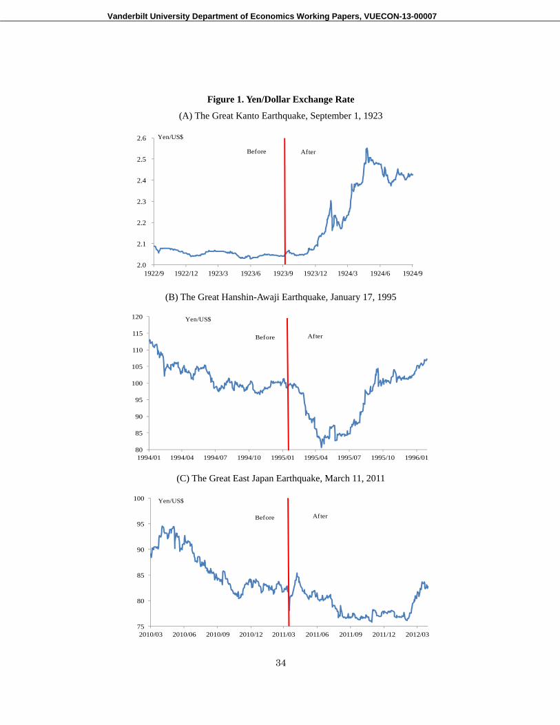
Vanderbilt University Department of Economics Working Papers, VUECON-13-00007
34
Figure 1. Yen/Dollar Exchange Rate
(A) The Great Kanto Earthquake, September 1, 1923
2.0
2.1
2.2
2.3
2.4
2.5
2.6
1922/9 1922/12 1923/3 1923/6 1923/9 1923/12 1924/3 1924/6 1924/9
Before After
Yen/US$
(B) The Great Hanshin-Awaji Earthquake, January 17, 1995
80
85
90
95
100
105
110
115
120
1994/01 1994/04 1994/07 1994/10 1995/01 1995/04 1995/07 1995/10 1996/01
Before After
Yen/US$
(C) The Great East Japan Earthquake, March 11, 2011
75
80
85
90
95
100
2010/03 2010/06 2010/09 2010/12 2011/03 2011/06 2011/09 2011/12 2012/03
Before After
Yen/US$

Vanderbilt University Department of Economics Working Papers, VUECON-13-00007
35
Figure 2. Yen/Dollar Exchange Rate and Target Rate
2.0
2.1
2.2
2.3
2.4
2.5
2.6
2.7
1922/4 1923/4 1924/4 1925/4
NY Close
Target
Before After
Yen/US$
Figure 3. Amounts of Intervention
-25
-20
-15
-10
-5
0
5
10
15
20
25
1922/4 1923/4 1924/4 1925/4
Sell $, buy yen
Buy $, sell yen
Before After$ 1mil
Figure 4. Foreign Exchange Reserves
0
50
100
150
200
1922/4 1923/4 1924/4 1925/4
Before After
$ 1mil