NBER WORKING PAPER SERIES

VALUING PAIN USING THE SUBJECTIVE WELL-BEING METHOD

Thorhildur ÓlafsdóttirTinna Laufey Ásgeirsdóttir

Edward C. Norton

Working Paper 23649http://www.nber.org/papers/w23649

NATIONAL BUREAU OF ECONOMIC RESEARCH1050 Massachusetts Avenue

Cambridge, MA 02138August 2017

The views expressed herein are those of the authors and do not necessarily reflect the views of the National Bureau of Economic Research.

NBER working papers are circulated for discussion and comment purposes. They have not been peer-reviewed or been subject to the review by the NBER Board of Directors that accompanies official NBER publications.

© 2017 by Thorhildur Ólafsdóttir, Tinna Laufey Ásgeirsdóttir, and Edward C. Norton. All rights reserved. Short sections of text, not to exceed two paragraphs, may be quoted without explicit permission provided that full credit, including © notice, is given to the source.

Valuing Pain using the Subjective Well-being MethodThorhildur Ólafsdóttir, Tinna Laufey Ásgeirsdóttir, and Edward C. NortonNBER Working Paper No. 23649August 2017JEL No. I10,I14

ABSTRACT

Chronic pain clearly lowers utility, but it is empirically challenging to estimate the monetary compensation needed to offset this utility reduction. We use the subjective well-being method to estimate the value of pain relief among individuals age 50 and older. We use a sample of 64,205 observations from 4 waves (2008-2014) of the Health and Retirement Study, a nationally representative individual-level survey data, permitting us to control for individual heterogeneity. Our models, which allow for nonlinear effects in income, show the value of avoiding pain ranging between 56 to 145 USD per day. These results are lower than previously reported, suggesting that the value of pain relief varies by income levels. Thus, previous estimates of the value of pain relief assuming constant monetary compensation for pain across income levels are heavily affected by the highest income level. Furthermore, we find that the value of pain relief increases with pain severity.

Thorhildur ÓlafsdóttirUniversity of IcelandFaculty of Business AdministrationOddi v. Sturlugotu101 ReykjavikIcelandthorhilo@hi.is

Tinna Laufey ÁsgeirsdóttirUniversity of IcelandDepartment of EconomicsOddi v. Sturlugotu101 ReykjavikIcelandta@hi.is

Edward C. NortonDepartment of Health Management and PolicyDepartment of EconomicsUniversity of MichiganSchool of Public Health1415 Washington Heights, M3108 SPHIIAnn Arbor, MI 48109-2029and NBERecnorton@umich.edu

Introduction

Chronic pain clearly lowers utility, but quantifying exactly how much people are willing to

trade off pain and income is challenging empirically. We use rigorous econometric methods

that avoid the problems of market-based valuation, stated-preference methods, and hedonic

wage methods. Instead we use the subjective well-being method, which uses the statistical

relationship between subjective well-being and health compared to the relationship between

subjective well-being and income. The method has been used extensively in evaluating well-

being, but relatively few published applications to health. However, with increased availability

of individual longitudinal survey data on subjective well-being and health, it has the potential

to improve previous values of health conditions derived from other methods.

The specific aim of this research is to estimate the monetary value of pain relief among

individuals age 50 and older, using the subjective well-being method. The obvious aim of pain-

relief treatment is to eliminate the welfare reductions associated with pain. Although there may

be other benefits, such as productivity gains (Kapteyn, Smith, & van Soesta, 2008), the direct

effect on quality-of-life is likely to be extensive and should thus not be overlooked. Monetizing

this welfare reduction is needed to choose financing of the treatment with the largest net benefit

or to choose between a new pain treatment and welfare-increasing policies in other sectors, for

which benefits have been estimated. Pain prevalence is higher in samples of older individuals

and chronic pain is associated with psychological distress, functional impairment and disability

(Hardt, Jacobsen, Goldberg, Nickel, & Buchwald, 2008; Nahin, 2015).

We contribute to the literature in four ways: First, by analyzing a dataset that is

exceptionally well suited for the research question and methods. Specifically, we study

detailed, longitudinal individual-level data on a sample for which pain is prevalent and we can

control for individual heterogeneity. Second, by exploring the methodology of the subjective

well-being method from a new perspective — using models that are more flexible by allowing

2

a piecewise-linear relationship in the income variable. Third, by addressing endogeneity, we

also provide results where income is instrumented, because theory and previous research

suggests a downward bias in the income variable without instrumentation. Finally, we test the

sensitivity of results to the level of pain severity.

We find that the value of pain relief varies by income levels. Previous estimates that

assume constant monetary compensation for pain across income levels are probably too high

because those are heavily affected by the highest income levels. We thus highlight that the

estimated value of pain is sensitive to the functional form of income in subjective well-being

equations. In addition to allowing for nonlinear effects in income, including individual fixed

effects in our models and instrumenting for income in some estimations allows us to infer that

the value of pain relief is lower than previous research suggests. Our findings furthermore

suggest that the value of pain relief increases with pain severity.

Conceptual framework

Because health care is generally partially or completely subsidized, the value of medical

treatment cannot be inferred simply by observing the behaviors of buyers and sellers in the

market. To overcome the lack of revealed preferences when valuing pain we estimate the

change in well-being following a change in pain status using a monetary measure from welfare

economics: An income-compensated money measure, often referred to as compensating

variation (CV) (Hicks, 1939). In particular, CV is the amount of money received by or from an

individual that leaves him at his original level of welfare following a welfare change. CVs are

calculated under the assumption that the indifference curve represents the constant-utility trade-

off between income (consumption) and the non-market good (pain).

The method used in this study relies on survey responses to a subjective well-being

question that is taken as a proxy for utility. In line with this literature, we consider the concepts

3

of subjective well-being, utility, happiness, life satisfaction, and welfare as interchangeable.

Developments in subjective well-being research (happiness research) over the past four

decades are reviewed in Frey and Stutzer (2002), Clark, Frijters and Shields (2008), DiTella

and MacCulloch (2006), Becchetti and Pelloni (2013) and Frey, Luechinger, and Stutzer

(2010).

Applications of the subjective well-being method to health using cross-sectional data

include severe headache and migraine (Groot & van den Brink, 2004), cancer, cardiovascular

disease, thyroid disease, arthritis and infectious disease (Rojas, 2009), cardiovascular disease

(Groot & van den Brink, 2006, 2007; Groot, van den Brink, & Plug, 2004) and EQ5D

conditions, pain and anxiety (Graham, Higuera, & Lora, 2011). Applications that use

longitudinal data with fixed-effects (FE) models include chronic diseases (Ferrer-i-Carbonell

& van Praag, 2002), 13 health conditions (Powdthavee & van den Berg, 2011), chronic pain

(McNamee & Mendolia, 2014) cardiovascular disease (Latif, 2012) and general health status

(Brown, 2015). Asgeirsdottir et al. (2017) and Howley (2017) use longitudinal data without

FE-models to value 34 and 15 health conditions, the latter controlling for variables that proxy

personality traits.

Other methods that have been used for non-market valuations are mainly either

contingent valuation, the most widely used of stated preference methods, or the hedonic wage

method, a revealed preference approach. The contingent-valuation method remains

controversial (Carson, Flores, & Meade, 2001). It is more likely to capture attitudes rather than

preferences whereof attitudes are more sensitive to situations, the focusing illusion and to the

scale-of-reference bias (Kahneman & Sugden, 2005). Comparison of the hedonic method to

the subjective well-being method has revealed that price differentials obtained from the

hedonic method (or wage differentials in the case of health risks) may only partly represent the

value being estimated (van Praag & Baarsma, 2005). Considering health risks, an example

4

being if physical or emotional transaction costs of changing jobs are high, the value of health

would not be reflected in wage differentials. Furthermore, those who take on risky jobs are

likely to evaluate their health systematically lower than others. One of the main advantages of

the subjective well-being method is that people are not aware that their responses will be used

to derive their preferences for health and thus strategic responses are highly unlikely.

Furthermore, this method puts less cognitive strain on individuals than the stated-preference

method because they do not have to express their choices in imaginary situations, irrelevant of

whether they have actually experienced the health condition under study or not.

It is beneficial to develop and use various methods of well-being evaluation so that they

can serve as robustness checks to each other to validate results before they are implemented in

policy. Comparison of estimates from subjective well-being measures to estimates from the

widely used time-trade-off method (TTO) has, for example, revealed that policy implications

can differ considerably between the two methods. Dolan and Metcalfe (2012) found that

through TTO preferences, being confined to bed is worse than having extreme anxiety but

using subjective well-being estimates, showed the opposite.

Although the subjective well-being method is a useful addition and even superior to

hypothetical preferences in valuing health, it is not without limitations (Becchetti & Pelloni,

2013; Clark et al., 2008; Luechinger, 2009). Possible biases in the coefficients of interest,

specifically income and pain, should be considered. This is due to a possible violation of the

zero-conditional-mean assumption; 𝐸(𝜀|𝑥) = 0, where 𝜀 is an error term in a regression model

and the regressor(s), 𝑥 thus are correlated with the error term because of a) simultaneous

determination of the dependent variable and regressors (or reverse causality), b) omitted

variables and c) measurement error in the regressors.

We address these potential biases in the following ways: First, individual fixed effects

models are used to control for unobserved time-fixed characteristics. Previous research using

5

FE-models report a positive personality-traits bias of the income and health coefficient in life-

satisfaction models without fixed effects (Ferrer-i-Carbonell & Frijters, 2004; McNamee &

Mendolia, 2014). Powdthavee (2010) reviews literature that suggests that extroverts do better

in the labor market and are happier. The same characteristics could also be associated with

being healthy. Second, by using last year´s reported income to address the possibility of life

satisfaction affecting income levels. Third, by analyzing a subsample of 65 years and older, we

make use of the proposition that income is plausibly exogenous in retirement as a function of

past values of the variables in the model. Finally, we report results from models where income

is instrumented with mother´s education, further addressing the endogeneity of income that

could cause a downward bias in the point estimate as well as to address possible measurement

error. A measurement error in a covariate biases its´ coefficient towards zero, given that

possible measurement errors on other regressors are independent (Cameron & Trivedi, 2005).

However the use of lagged income to address endogeneity at time t is open to objections

because of the adaptation argument that the current level of life satisfaction is not independent

of income in the previous time periods (Di Tella, Haisken-De New, & MacCulloch, 2010).

We also note that the income coefficient could be biased downward if leisure

(Kahneman, Krueger, Schkade, Schwarz, & Stone, 2004) or other people´s income

(aspirations) are not controlled for (Easterlin, 2005; Luttmer, 2005; McBride, 2001). This

would result because of the negative correlation between income and leisure on one hand and

the positive correlation between income and aspirations on the other hand, combined with the

positive effect of leisure on life-satisfaction and the negative effect of aspirations on life-

satisfaction. Ferreira and Moro (2010) experimented with including estimates of relative

income (the difference between one´s own income and the average income of the local

authority of residence) in their models when valuing air quality and warm climate but excluded

the variable as it was not statistically significant. To summarize, it should be kept in mind that

6

estimated welfare measures from models that cannot compensate well for violation of the zero-

conditional-mean assumption may be an overestimate of the true compensation needed to make

an individual indifferent between having and not having a sub-optimal health condition.

Researchers have experimented with various instrumental variables (IVs) for income in

the subjective well-being literature. Examples include father´s years of education and spouse´s

years of education (Knight, Song, & Gunatilaka, 2009), and industry and occupation, Luttmer

(2005). The IV income coefficient was four times larger than the one obtained in the baseline

happiness estimation in the former study and instrumenting for income resulted in a threefold

coefficient in the latter study. However, the income coefficients are likely upward biased by

unobserved heterogeneity in both studies as the former use cross-sectional data and FE models

are not used in the latter. Powdthavee (2010) used exogeneous over-time variation in the

proportion of household members with payslip information for income instruments and reports

a FE-IV income coefficient that is double the size of the OLS coefficient and ten times larger

than the FE coefficient on income. Ambrey and Fleming (2014) used lottery winnings among

other irregular sources of income as IVs for income and their results also suggest that OLS

estimates lead to an overestimate of willingness to pay (WTP) for improved physical health.

Howley (2017), being the first study to use IV estimates in a health application of the subjective

well-being method, used parental education to instrument for income and found the income

coefficient to more than triple in size between OLS and two-stage least squares (2SLS) models.

With the subjective well-being method, respondents are never asked to state a monetary

value for pain. However, what is implicitly obtained is an answer to the question: “Considering

your overall satisfaction with life without being troubled by pain, how much money must we

pay you to make you just as happy even though you were often troubled by pain?” Or the other

way around: “Consider your overall satisfaction with life being often troubled by pain, what

7

would you be willing to pay to be just as happy but without pain?” Yet, the method does not

require respondents to actually deal with this cognitively difficult question.

8

Data

To estimate the monetary value of pain using the subjective well-being method, we need

person-level data with measures of life satisfaction, income, pain, and detailed controls for

health status. In addition, we want a population for whom pain is prevalent and income is

plausibly exogenous. Furthermore, to the extent that observations are missing person-level

time-invariant health status, we want longitudinal data so that identification can come from

within-person variation in income and pain, thus avoiding confounding by unobserved time-

invariant variables.

The Health and Retirement Study (HRS) has all of these features. We use data from the

four waves (2008, 2010, 2012 and 2014) of the HRS that include a question on life satisfaction.

The HRS is a biannual nationally-representative panel survey that started in 1992, on the health

and economic well-being of adults over 50 in the United States, including around 22,000

Americans per wave. The HRS is sponsored by the National Institute on Aging (grant number

NIA U01AG009740) and the Social Security Administration and is conducted by the

University of Michigan´s Institute for Social Research.

All variables used in the analyses are data products of the RAND Center for the Study

of Aging. Those variables were either cleaned and processed variables described in the RAND

HRS DATA FILE (v.P) (Bugliari et al., 2016) with model-based imputations, or variables from

the RAND Enhanced Fat Files (questions on life satisfaction and pain), with household data

merged to the respondent level.

The original sample using four waves consisted of 78,553 observations on 24,967

individuals. Of those, we excluded individuals under 50 years old and those living in a nursing

home. We also dropped observations that had missing values on the dependent and independent

variables. Because income is highly skewed and potentially mis-reported, we used the

condition DFbeta>1 to identify the overly influential observations on the income variable

9

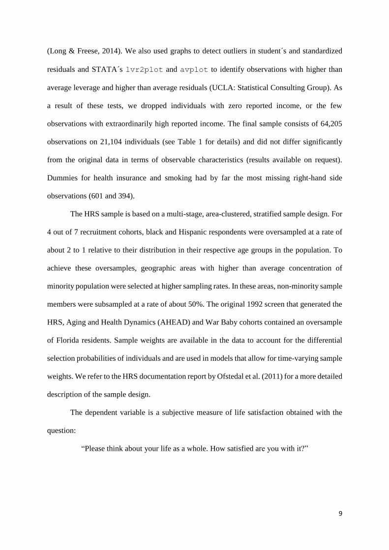
(Long & Freese, 2014). We also used graphs to detect outliers in student´s and standardized

residuals and STATA´s lvr2plot and avplot to identify observations with higher than

average leverage and higher than average residuals (UCLA: Statistical Consulting Group). As

a result of these tests, we dropped individuals with zero reported income, or the few

observations with extraordinarily high reported income. The final sample consists of 64,205

observations on 21,104 individuals (see Table 1 for details) and did not differ significantly

from the original data in terms of observable characteristics (results available on request).

Dummies for health insurance and smoking had by far the most missing right-hand side

observations (601 and 394).

The HRS sample is based on a multi-stage, area-clustered, stratified sample design. For

4 out of 7 recruitment cohorts, black and Hispanic respondents were oversampled at a rate of

about 2 to 1 relative to their distribution in their respective age groups in the population. To

achieve these oversamples, geographic areas with higher than average concentration of

minority population were selected at higher sampling rates. In these areas, non-minority sample

members were subsampled at a rate of about 50%. The original 1992 screen that generated the

HRS, Aging and Health Dynamics (AHEAD) and War Baby cohorts contained an oversample

of Florida residents. Sample weights are available in the data to account for the differential

selection probabilities of individuals and are used in models that allow for time-varying sample

weights. We refer to the HRS documentation report by Ofstedal et al. (2011) for a more detailed

description of the sample design.

The dependent variable is a subjective measure of life satisfaction obtained with the

question:

“Please think about your life as a whole. How satisfied are you with it?”

10

Respondents could choose an answer on a scale from 1 (“completely satisfied”) to 5 (“not at

all satisfied”). We reversed the scale so that 5 represents “completely satisfied”. Most people

report high satisfaction with life (see Figure 1 for the full distribution by pain status).

The independent variables of interest are real household income (reported in wave t for

wave t–1) and an indicator for whether the respondent is often troubled by pain. The question

on pain used in our main models is:

“Are you often troubled with pain?”

Respondents answered either yes or no. For those who answered yes, the survey also includes

a question on severity of pain with answer options: Mild, moderate, or severe. We use this

variable to test whether the estimated CVs are sensitive to degree of pain severity.

The question on pain does not explicitly distinguish between acute pain and chronic

pain. However, according to a study by Banks et al. (2009) we can assume that responses to

the HRS pain question reflect pain that is recurrent and not completely relieved by medication

(or alternative treatment). They compared two questions on pain that 2,000 respondents, 25

and older from the Dutch CentERpanel survey answered. One was the HRS pain question and

another question asked whether they had experienced any pain in the last 30 days. 59% of the

sample reported having “any pain in the last 30 days” but only 27% of the same sample reported

being “often troubled by pain” (the HRS question). This suggests that those who reported being

often troubled by pain are referring to recurrent pain, not short-term or acute pain that may be

fully alleviated from pain. The type of pain that people are queried about with the HRS question

is thus likely to be comparable to questions on chronic pain from other studies. As an example,

McNamee and Mendolia (2014) used data from the Australian HILDA Survey in their

estimation of the value of pain. They used responses from questions on whether individuals

had any long-term health conditions, with chronic pain as one of the possible alternatives over

a period of ten survey-waves.

11

The most common clinical definition of pain was introduced by the International

Association for the Study of Pain in 1979 (IASP Subcommittee on Taxonomy, 1979) as “an

unpleasant sensory and emotional experience associated with actual or potential tissue damage,

or described in terms of such damage”. The definition appreciates the multidimensional nature

of pain as it takes into account both physiological processes and the subjectivity of pain

experience. From a methodological perspective, the clinical definition of pain thus enforces the

reasoning to control for individual heterogeneity as time-invariant personality traits are likely

to simultaneously affect the subjective experience of both life satisfaction and pain.

The income variable is an all-inclusive sum of previous year´s wage and salary income,

bonuses, business income, asset income, pensions, benefits, compensations, and inheritance.

Total equivalised household income at the 2015 price level was calculated for each observation.

We use the modified OECD scale to equivalise household income where the first adult has

weight=1, the second adult in the household has weight=0.5 and children have weight=0.3. The

total household income only includes income from the respondent and the spouse, not from

other household members but a possible underestimation of household income is not

considered a problem because of this, as intergenerational transfers generally do not flow from

children to parents.

Other covariates are factors that are plausibly correlated with chronic pain and income

and are listed in Table 2, for the whole sample and by pain status. Those include indicators for

various health conditions as pain can be a consequence of those conditions. We chose

conditions asked about in the survey in the following manner, thus validating the variables as

much as possible: “Has a doctor ever told you that you have a ....?” querying about cancer, lung

disease, heart disease, stroke, psychological condition, arthritis and high blood pressure. Other

time-varying covariates included are: Age, marital status, labor-force status, health-insurance

status, wave dummy (capturing period-specific effects), smoking dummy and number of

12

children. Time-invariant covariates include gender, race, education, and census division. We

include age in our models in 5-year ranges even though age effects would be captured by the

time dummies if age was excluded. This is done because there is growing evidence from large

cross-sectional studies as well as longitudinal analyses that life satisfaction is affected

differently by age-groups, with a U-shaped relationship between well-being and age

(Blanchflower & Oswald, 2008; Cheng, Powdthavee, & Oswald, 2017), although the exact

form of the relationship is controversial. Studies have found well-being to decline after age 60

(Wunder, Wiencierz, Schwarze, & Kuchenhoff, 2013) and after age 75 (Frijters & Beatton,

2012) and some researchers report the reverse of a U-shape (Easterlin, 2006; Sutin et al., 2013).

Furthermore, the age variable controls for deterioration in health capital (Grossman, 1972) that

is not captured by the health condition dummies. We control for health-insurance status as

health insurance is found to be welfare-increasing from mid-life (Pelgrin & St-Amour, 2016).

The variable on marital status partly controls for relational goods, including companionship

and emotional support (Becchetti & Pelloni, 2013).

Methodology

Define indirect utility (𝑉) as a function of income (𝑦), health (ℎ), and a set of demographics

and personal characteristics (𝑥):

𝑉(𝑦, ℎ, 𝑥) (1)

Consider a reduction in health from ℎ1 to ℎ0, such that ℎ1>ℎ0, with no changes to 𝑦 or 𝑥. A

change in utility because of a change in health is then defined as follows:

∆𝑉 = 𝑉(𝑦, ℎ0|𝑥) − 𝑉(𝑦, ℎ1|𝑥) (2)

Then, the compensating variation (𝐶𝑉) is the amount of money that equalizes the individual´s

utility before and after the change in health so that:

𝑉(𝑦 + 𝐶𝑉|ℎ0, 𝑥) = 𝑉(𝑦|ℎ1, 𝑥) (3)

13

The empirical well-being equation is as follows:

𝑉𝑖𝑡 = 𝛽𝑜 + 𝛽1𝑦𝑖𝑡 + 𝛽2ℎ𝑖𝑡 + ∑ 𝛼𝑘𝑋𝑘,𝑖𝑡𝐾𝑘=1 + 𝜀𝑖𝑡 (4)

where 𝑉𝑖𝑡 in our case is reported life satisfaction of individual i at time t, and our health variable

h is pain. The alphas and betas are coefficients and the K variables 𝑋𝑘,𝑖𝑡 are demographics and

personal characteristics. 𝜀𝑖𝑡 is a composite error term for individual time-invariant

characteristics and time-varying characteristics for individual i at time t. We then use equation

(4) and solve for CV in (3), which results in the negative ratio of the coefficients for pain and

income:

𝐶𝑉 = −𝛽2

𝛽1 (5)

Estimation of the parameters in equation (4) and the corresponding CV in equation (5)

involves several econometric issues. First, the correct functional form of the covariate income

is not necessarily linear, as is assumed in equation (4). Therefore, we consider alternative, more

flexible, functional forms that allow the CV to vary at different levels of income. Similarly, in

some specifications we allow pain to have four values, including no pain, to indicate some

measure of pain intensity instead of just the binary indicator for frequent pain or not. Second,

repeated observations for each person allows the use of panel-data methods to control for time-

invariant factors and to identify the two main coefficients using within-person variation. Third,

because the data are collected from a survey, subjects are sampled with unequal weights. We

explore whether weighted estimates differ from unweighted estimates. Fourth, we attempt to

separate the life-satisfaction effects of pain itself from the underlying health conditions that

might cause them with carefully selected health controls. Fifth, although we attempt to control

for all possible confounders, including using person-level fixed effects, there is still the

possibility that either income or pain (or both) are correlated with unmeasured factors that also

affect happiness. An example of such a variable is unmeasured health status. Therefore, we

also estimate models that use instrumental variables to control for endogeneity. Sixth, we test

14

whether the results are sensitive to inclusion of additional covariates. Seven, we test for

heterogeneous treatment effects by estimating the models on subsamples by age and gender.

We explore each of these issues in more detail below.

We let the continuous variable income enter equation (4) in three different ways: linear,

log-transformed and piecewise linear (PWL). Previous studies using the subjective well-being

method use either linear income or more commonly its logarithmic transformation. The log

transformation is used to model diminishing marginal utility of income citing Layard, Nickel

and Mayraz (2008) but also to reduce effects of influential observations in the income

distribution characterized by right skewness. We therefore highlight the empirical and

theoretical reasons for those results, although we also report linear income results for reason of

comparability between studies, as well as to compare results using different model

specifications.

In models with the log transformation of income, the coefficient ratio compares

marginal changes in pain to marginal changes in % income. Thus calculating CV calls for

reverting the proportion of coefficients for pain and income from the logarithmic scale by using

the exponential function. Thus, replacing income with ln(income) in (4) and solving for CV in

(3) yields:

𝐶𝑉 = �̅� (𝑒𝑥𝑝 (−𝛽2

𝛽1) − 1) (6)

where �̅� is average income in the sample. We report CVs as daily monetary amount and since

the income variable is in 10,000 USD,

𝐶𝑉 𝑝𝑟. 𝑑𝑎𝑦 𝑖𝑛 𝑈𝑆𝐷 = (𝐶𝑉 ∗ 10,000)/365 (7)

This amount is interpreted as the additional equivalised household income per day

needed to compensate an individual who often suffers from pain for his/her loss in welfare

(willingness to accept (WTA)) or as the equivalised income per day that he/she is willing to

forgo to be relieved from pain (WTP).

15

Although using ln(income) generally provides a better fit than using linear income, it is

not helpful for exploring differences in CV by income levels. Another option that does not

impose the exact same tradeoff between income and pain across all income levels (as the linear

case does) is to use a piecewise linear functional form for income. CVs from PWL models are

calculated the same way as in the case of linear income for each income spline (see equation

(5)).

We estimate CVs from individual FE models in addition to OLS and OLS-PWL models

because previous research suggests that fixed effects play an important role in well-being

equations (Ferrer-i-Carbonell & Frijters, 2004; McNamee & Mendolia, 2014). These models

identify the parameters on income and pain through within-person variation in those variables,

instead of cross-sectional variation. Models were weighted where possible, to account for the

complex multistage probability survey design. This includes non-response, sample clustering,

stratification and further post-stratification. Models with and without weights yielded quite

similar results, relieving our concerns of not being able to include sampling weights in FE-

models. For ease of comparison between models, we thus report unweighted results in the

results tables but provide results from weighted regressions in an Appendix.

Using goodness-of-fit test statistics, the Akaike information criterion (AIC) and the

Bayesian information Criterion (BIC), the piecewise linear (PWL) specifications consistently

showed a better fit to the data than the transformation of income to logarithm scale. Nonlinear

least-squares estimates were used to suggest a breakpoint combined with goodness of fit

statistics, AIC and BIC, to choose from different sets of breakpoints. The choice of breakpoints

was at 30,000 and 50,000 USD (annual income), corresponding to the 51st and 72nd percentiles

of the income distribution. We report tests for differences in the spline coefficients between

the first and second segments in the PWL-OLS model (see Table 3 of the results section).

Figure 2 shows the relationship between income and life satisfaction using a non-parametric

16

smoother and a fitted piecewise-linear function of income with the chosen knots marked by the

horizontal lines. We include only income below 300,000 USD in the figure for better visibility

of the difference in the slope of the function at income levels, where the marginal utility of

income (non-adjusted) is proportionally large over the income distribution.

In addition to results from OLS, piecewise-linear and FE models, we provide results from

2SLS models with mother´s education as an instrument for income. The relevance of our

control variables was confirmed by comparing results from unadjusted models, which include

only pain and income on the right hand side of equation (1), to adjusted models that include all

independent variables as feasible for each model estimator. As a robustness check of our CV

estimates, we report results from analyses of a subsample of people age 65 and above because

it is more plausible to think of income as an exogenous variable in a model with this age group.

Previous research has reported gender differences in CVs (Groot & van den Brink, 2006;

McNamee & Mendolia, 2014) and we provide results by gender for completeness. Further,

estimates with pain severity instead of the pain dummy are included since the CVs are likely

to be sensitive to whether pain is mild, moderate or severe.

Results

Results for the total sample are reported in Table 3, results by gender in Table 4 and results for

the subgroup of 65 years and older in Table 5. Point estimates for pain and income by estimator

and functional specification of income are reported along with corresponding CV estimates.

Results are presented from models where income is used in a linear and piecewise-linear form

in panels A. In panel B, we present results from models with log of income. As an example,

looking at Table 3, the CV estimate in the first column, panel A is the negative ratio of the two

reported coefficients (see equation (2)) and can be interpreted as the additional equivalised

household income per day in USD that would be needed to compensate an individual for the

welfare loss of often suffering from pain.

17

The results reported in column one, Table 3, assume that the CV is constant across all

income levels, an assumption that is both restrictive and testable. In contrast, results in column

2 allow the CV to differ across three different income ranges. That result shows that the CV is

much larger for those with income above $50,000. Furthermore, comparing panel A and B in

column one, the calculated CV with ln(income) is 2.6 times larger than when income enters

the model in linear form. This large difference calls for further exploration of the functional

form of the income variable. By including income in the empirical model in linear splines, a

CV estimate is directly observable for income splines that capture the part of the income

distribution representing the majority of individuals in the population. That is, CV estimates

from the first and second segments of the spline regression reflect the marginal rate of

substitution between income (consumption) and pain at levels below the 72nd percentile of the

income distribution. Thus, the value of pain differs by income levels. It ranges from 95 to 1,720

USD per day using OLS models. Even though the CIV for the third spline from the PWL-OLS

model is statistically significant at the 1% level, the volatility in life-satisfaction predictions

increases drastically at income levels above 300,000 USD (see Figures A1-A3 in Appendix).

That is, the estimated CVs in columns one of Tables 3-5, are likely to be heavily affected by

the trade-off between income and pain at the highest income levels.

Results from FE models confirm the positive personal traits bias in OLS models

reported in previous research since the coefficients decrease in absolute value. However, the

CV estimate is only statistically significant in the FE model in the case of linear income (panel

A). The standard errors of the CV estimates are calculated by the delta method in STATA and

in the FE model in panel B this results in proportionally large standard errors with this data. In

column four (PWL-FE model), the estimated CV from the second segment is statistically

significant and similar to the CV estimate from the PWL-OLS model. The reason for zero effect

of income in the FE-spline regression is the lack of within-variation in the first and third income

18

splines. However, as this estimator works well for the second spline of the income distribution,

we include it for reasons outlined in the methodology section on preference for FE-models in

the literature. Comparing CV estimates from PWL-OLS and PWL-FE models, the estimated

CV from the second segment is statistically significant in both models (95 USD in PWL-OLS

and 56 USD in PWL-FE model) suggesting a much smaller CV than estimates from models

with ln(income) (Panel B) and from the third segment of the spline regressions.

We point out that precision in fixed-effects models is contingent on the within-variation

in the variables used and we explored this in our data. 12,461 individuals change status in the

life-satisfaction variable, 6,421 change status in the pain variable and 18,421 change status in

the income variable during the observation period. This resulted in only 4,546 individuals

changing status in all three variables. By using spline regression, this resulted in 3,238

individuals at the most changing status in life satisfaction, pain and first income spline (1,819

if conditional on change in third income spline). This explains the large standard errors in PWL-

FE models for the first and third income splines.

Our results from fixed-effects models are similar to those from McNamee and Mendolia

who used fixed effects models with log of income and found the daily CV for pain nine times

the average income per day using Australian data. Our results suggest that an individual with

average equivalised total household income of 125 USD per day would need extra USD of

1,040 per day to achieve the same level of life satisfaction as someone who is not often troubled

with pain or eight times the average equivalised household income per day. Graham et al.

(2011) found CV for extreme pain to be five times the income for the corresponding period

using cross-sectional data. Results from piecewise-linear models however suggest a much

smaller CV for pain than previous research or compensation of as low as 56 USD per day.

19

The last column, displays estimates from 2SLS models. We explored the three possible

instruments for income available, as suggested by previous research; mother´s education,

father´s education and spouse´s education, (Howley, 2017; Knight et al., 2009). For an

instrument to be relevant it has to be highly correlated with income and to be valid it must have

no partial effect on life satisfaction, after conditioning on the other included variables (and

individual fixed effects in the FE models). Spouse´s education did not pass the test of relevance

in the first stage and was therefore discarded. Both father´s and mother´s education was

relevant based on F-test of excluded instruments from the first stage. However, father´s

education did not pass the test of weak-instrument robust inference (Anderson-Rubin Wald

test), which can cause an IV estimate to exhibit greater bias than OLS estimate (Bound, Jaeger,

& Baker, 1995). Furthermore, as correlation between father´s and mother´s education was high

(ρ=0.68), adding the second instrument in this case would not add much information to produce

the slope estimate as opposed to having only the one chosen. Thus, we instrument for income

with mother´s education; the highest grade completed in school. This variable has a significant

relationship of the expected sign with the income variable with F-test of the excluded

instrument equal to 80 (a conventional minimum of this F-test is> 10) (Stock, Wright, & Yogo,

2002). The null hypothesis of B1 of the endogenous regressor in the structural equation being

equal to zero was furthermore rejected (p=0.0009) (Anderson-Rubin Wald test, as described in

Baum, Schaffer, & Stillman (2007)). The H0 of whether the endogenous variable can be treated

as exogenous was rejected (p=0.0047 for the linear income model and p=0.0183 for the

ln(income) model). The positive relationship between mother´s education and later

achievements of her children, including their income as adults is well documented. Better

educated mothers are likely to have greater resources when it comes to helping their children

with homework and thereby facilitating educational achievement and higher income of their

children later in life. Mother´s education may also assist her children in the labor market

20

through social status and networks. We refer to Howley (2017) for a review of the literature

supporting the relevance of our instrument. We assume that the variance in life satisfaction

explained by variation in income is attributable solely to the variance in mother´s education

(the exclusion restriction). In other words, the exclusion restriction asserts that mother´s

education is only related to her child´s life satisfaction through child´s income as adult. Doubts

on the legitimacy of this statement may be such that children of higher educated mothers are

endowed with personal skills that are positively correlated with income, health, labor-market

status and marital status, all of which are related to life satisfaction. However, as we control

for such channels in our empirical model as well as individual time-fixed characteristics, we

can reasonably oppose doubts based on such channels.

The downward bias of the income coefficient in models without instruments, as

documented in previous research is likely explained by willingness to substitute leisure for

working hours now as investment for future happiness, thereby increasing income at the

expense of current happiness. Another explanation is that the 2SLS estimator corrects for an

attenuation bias as a result of measurement error in the income variable. Furthermore, as

reviewed by Powdthavee (2010), not being able to control for other people´s income or rate of

adaptation and aspiration to income may cause this downward bias.

Compared to the OLS results, the income coefficient is 6.6 times larger in the model

with instrumented income. This is a larger increase than in previous research. The calculated

CV of 129 USD per day (Table 3, panel A) may however still be biased by unobserved

individual heterogeneity as we could not estimate FE-IV models as mother´s education is time-

invariable. Considering the proportional reduction of the coefficients for pain and income once

individual fixed effects are controlled for (compare coefficients in first and third column) of

73% for the pain coefficient and 76% for the income coefficient and applying those to the

21

coefficients from the 2SLS model in column five results in a CV estimate of 145 USD per day,

an amount extremely close to the CV estimates of 129 in panel A and 152 in panel B.

Results by gender are reported in Table 4. We only display results by gender from OLS,

FE and 2SLS models for reason of parsimony. Results from piecewise-linear models were

similar by gender (results available upon request). The estimated CVs are similar for men and

women in panel A but the CV estimate from the OLS model in panel B for women is larger

than men´s by 1,067 USD per day. Results from 2SLS suggest a much larger CV for men than

for women, explained by smaller marginal utility of income for men in column three of Table

4.

The results for the subsample of 65 years and older are shown in table 5. In general, the

results are in line with the results for the full age sample in Table 3, in particular for OLS,

PWL-OLS and OLS-IV models. Results from the PWL model reflect that the slope of the

indifference curve between pain and income depends on income level. CV estimates from FE

models have large standard errors and this may be due to less within-individual variation in

income (and/or life satisfaction) in a restricted sample. This is in accordance with one or both

of the following: (a) our proposition of income being fairly exogen for those 65 and older is

not supported by those results, especially in light of the similar results from the models where

we instrument for income or (b) income is generally fairly exogenous in life-satisfaction

models, but the 2SLS estimations are mainly correcting biases due to other factors, such as

measurement errors and omitted variable biases described above.

Finally, we explored the sensitivity of the estimated CVs to the severity of pain. As

would be expected, the monetary amount needed to compensate for welfare losses due to pain

suffering increases by level of pain severity (see Table 6).

We provide results tables in an Appendix that include all coefficients for OLS, FE and

OLS-IV models (Table A1 and A2). Looking at results from the FE model, the coefficients are

22

of the expected sign and in accordance with previous research. Unemployed are less satisfied

with life than the employed or those out of the labor force. Retired are happier than the

employed. Being married is preferred to being divorced, widowed or single. Number of

resident children does not affect life satisfaction. Having ever reported cancer, heart problems,

stroke, psychological problems or high blood pressure is negatively related to life satisfaction

with psychological problems standing out as having the largest negative effect. It is preferred

to have health insurance and surprisingly to smoke. However, life satisfaction is not affected

over time ceteris paribus except for a small decrease in life satisfaction between 2008 and 2010.

Life satisfaction increases with age at a diminishing rate with a decline in life satisfaction

starting at age 70 (in accordance with U-shaped relationship between life-satisfaction and age

in samples including all ages as our sample includes 50 years and older). Comparison of

unadjusted and adjusted (all controls included) models revealed that as expected, the

coefficients for chronic pain and income decrease when more control variables are added in

the OLS models but stay mostly unchanged in the FE models, suggesting that the fixed effects

capture an important part of the relationship between pain and life satisfaction on one hand and

income and life satisfaction on the other (see Table 3A in Appendix). We note that results in

Tables 3 to 6 are unweighted for ease of comparison as it was not possible to use weights in

the FE models. Comparison of weighted and unweighted results yielded similar results for

other models (see Table A4 in Appendix).

Discussion

The results in this paper add new information on the value of pain relief among people older

than 50 years old. Using improved methods, our results suggest a lower CV for pain than

previously reported. More importantly, we contribute to the literature in a novel way by using

a PWL model as an alternative to OLS with ln(income), providing a more transparent method

to express WTP/WTA across income ranges. The resulting CV-estimates are lower than those

23

from models using the traditional log transformation of income. Results from IV-models also

yield CVs that are considerably lower than previous research suggests.

We point out that even though the results show that higher monetary compensation is

needed to offset the utility loss of often having pain for richer individuals than for lower-income

individuals, it does not imply that society has to value the health of richer individuals more

than that of poorer ones. It simply reflects the general assumption that the marginal utility of

income is larger for low-income individuals than for high-income individuals. As expected,

CVs are also found to be positively related to pain severity.

McNamee and Mendolia’s (2014) CV estimate for chronic pain was 640 USD per day

using ln(income) in FE models. We were not able to produce a reliable CV estimate from a

comparable model but our CV estimate using FE model with linear income was 1,040 USD

per day. Their sample differs from ours in a number of ways. They use data from 10 waves of

the Household, Income, and Labor Dynamics of Australia Survey (HILDA) as opposed to 4

waves used in the current study, mean age in their sample is 45 as opposed to 68 in our sample

and covariates are not identical. Their use of longer panel helps with identification and

precision of point estimates but should not affect the size of the CV estimates. Prior studies

(Graham et al., 2011; McNamee & Mendolia, 2014) do not report standard errors for estimates

of CV, as we do, which makes comparison even more difficult. The large difference in CV

estimates by income levels, clearly displayed with PWL-models with and without fixed effects,

combined with results from 2SLS shed new light on the value of relief from chronic pain —

being lower than previous results suggest or in the range of 56 to 145 USD per day (using CV

estimates from panel A, column three and column four, with the latter adjusted for upward

personality bias suggested by comparison of coefficients from OLS and FE models).

Our paper also has several methodological conclusions. Although a distinction is made

between CV and EV in theory we can´t make a distinction between the two with the estimation

24

method used. The same applies to differentiating between WTA and WTP. Therefore, we guide

the reader on how to interpret the results acknowledging the limitations of the method in

identifying exactly what is being measured according to price theory.

Comparing estimates from linear income and log income models, the CV-estimates

should not be numerically the same but one cannot say a priori exactly how they should differ.

Taking the log of income, applying the exponential function to the ratio of the coefficients and

multiplying with mean income does not give the same results as using linear income. The linear

splines allow for exploring explicitly different CVs by income levels. For that reason, along

with a better model fit it is arguably better than taking log of income.

Our paper has several limitations. Pain can be a consequence of neurological diseases,

diabetes, or of musculoskeletal origin, but we did not have controls for those conditions that

we found validated by a doctor´s diagnosis. We acknowledge the possibility of a bias in the

coefficient for pain because of not being able to isolate the true effect of pain on life satisfaction

completely, but we assume that a possible omitted variable bias in the pain coefficient is

captured by controlling for age as neurological disease and diabetes likelihood increases with

age (referring to diabetes Type II). Furthermore, the other health controls included are likely

to capture the effect of musculoskeletal conditions on pain and life satisfaction, in particular

psychiatric problems, lung disease, cancer and arthritis.

Responses to life-satisfaction questions may be liable to situational influences, such as

the site of the interview, the weather, one´s mood and the interviewer, but those differences

can be considered as random error (Veenhoven, 1993). Life-satisfaction scores have been

found to correlate with variables that can be claimed to reflect utility, such as length of life and

mental health. Furthermore, happiness scores are highest in countries with most material

comfort, social equality, political freedom and access to knowledge (Veenhoven, 1993).

Developments within the subjective well-being literature have resulted in the use of questions

25

and terms that have been found to produce valid and reliable responses to measure utility, one

being the satisfaction-with-life question framed in a way so that the question makes clear that

life as a whole is to be considered. Life satisfaction is assumed to refer to a conscious global

judgement of one´s life but life-satisfaction scores may also reflect current affect, adding noise

to it as a measure of true experienced utility (Diener, 1984). Citing Ditella and MacCulloch

(2006): “Ultimately, happiness research takes the view that happiness scores measure true

internal utility with some noise, but that the signal-to-noise ratio in the available data is

sufficiently high to make empirical research productive”. The validity of the assumption of

interpersonal comparisons has been discussed thoroughly in the life-satisfaction literature with

the consensus that the responses, although not without their problems, are meaningful and

reasonably comparable among groups of individual (Easterlin, 2005).

We have learned that the value of pain is likely overestimated in previous research, with

our best approximation to a WTP/WTA estimate being in the range of 56-145 USD per day.

Furthermore, as expected, the data confirms that the value of pain relief is positively related to

severity of pain. CVs calculated with linear income are likely to result in overestimates and

PWL estimations are promising as they perform well econometrically in this context and allow

for easier exploration of results across income groups than log transformations of income.

26

References

Ambrey, C. L., & Fleming, C. M. (2014). The causal effect of income on life satisfaction and

the implications for valuing non-market goods. Economics Letters, 123(2), 131-134.

doi:http://dx.doi.org/10.1016/j.econlet.2014.01.031

Asgeirsdottir, T. L., Birgisdottir, K. H., Ólafsdóttir, T., & Olafsson, S. P. (2017). A

compensating income variation approach to valuing 34 health conditions in Iceland.

Economics & Human Biology, 27, 167-183.

doi:http://dx.doi.org/10.1016/j.ehb.2017.06.001

Banks, J., Kapteyn, A., Smith, J. P., & Van Soest, A. (2009). Work disability is a pain in the

****, especially in england, the Netherlands, and the United States. In D. Cutler & D.

Wise (Eds.), Health in older ages: The causes and consequences of declining

disability among the elderly

Cambridge, MA: NBER.

Baum, C. F., Schaffer, M. E., & Stillman, S. (2007). Enhanced routines for instrumental

variables/generalized method of moments estimation and testing. Stata Journal, 7(4),

465-506.

Becchetti, L., & Pelloni, A. (2013). What are we learning from the life satisfaction literature?

International Review of Economics, 60(2), 113-155. doi:10.1007/s12232-013-0177-1

Blanchflower, D. G., & Oswald, A. J. (2008). Is well-being U-shaped over the life cycle?

Social Science & Medicine, 66(8), 1733-1749. doi:10.1016/j.socscimed.2008.01.030

Bound, J., Jaeger, D. A., & Baker, R. M. (1995). Problems with Instrumental Variables

Estimation When the Correlation between the Instruments and the Endogenous

Explanatory Variable Is Weak. Journal of the American Statistical Association,

90(430), 443-450. doi:Doi 10.2307/2291055

Brown, T. T. (2015). The Subjective Well-Being Method of Valuation: An Application to

General Health Status. Health Services Research, 50(6), 1996-2018.

doi:10.1111/1475-6773.12294

Bugliari, D., Campbell, N., Chan, C., Hayden, O., Hurd, M., Main, R., . . . Clair, P. (2016).

RAND HRS Data Documentation, Version P. Retrieved from

Cameron, A. C., & Trivedi, P. K. (2005). Microeconometrics. New York: Cambridge

University Press.

Carson, R. T., Flores, N. E., & Meade, N. F. (2001). Contingent valuation: Controversies and

evidence. Environmental & Resource Economics, 19(2), 173-210. doi:Doi

10.1023/A:1011128332243

Cheng, T. C., Powdthavee, N., & Oswald, A. J. (2017). Longitudinal Evidence for a Midlife

Nadir in Human Well-Being: Results from Four Data Sets. Economic Journal,

127(599), 126-142. doi:10.1111/ecoj.12256

Clark, A. E., Frijters, P., & Shields, M. A. (2008). Relative income, happiness, and utility: An

explanation for the Easterlin paradox and other puzzles. Journal of Economic

Literature, 46(1), 95-144. doi:DOI 10.1257/jel.46.1.95

Di Tella, R., Haisken-De New, J., & MacCulloch, R. (2010). Happiness adaptation to income

and to status in an individual panel. Journal of Economic Behavior & Organization,

76(3), 834-852. doi:10.1016/j.jebo.2010.09.016

Di Tella, R., & MacCulloch, R. (2006). Some uses of happiness data in economics. Journal

of Economic Perspectives, 20(1), 25-46.

Diener, E. (1984). Subjective Well-Being. Psychological Bulletin, 95(3), 542-575. doi:Doi

10.1037//0033-2909.95.3.542

27

Dolan, P., & Metcalfe, R. (2012). Valuing Health: A Brief Report on Subjective Well-Being

versus Preferences. Medical Decision Making, 32(4), 578-582.

doi:10.1177/0272989x11435173

Easterlin, R. A. (2005). Building a better theory of well-being. In L. Bruni & P. L. Porta

(Eds.), Economics and happiness. New York: Oxford University Press.

Easterlin, R. A. (2006). Life cycle happiness and its sources - Intersections of psychology,

economics, and demography. Journal of Economic Psychology, 27(4), 463-482.

doi:10.1016/j.joep.2006.05.002

Ferreira, S., & Moro, M. (2010). On the Use of Subjective Well-Being Data for

Environmental Valuation. Environmental & Resource Economics, 46(3), 249-273.

doi:10.1007/s10640-009-9339-8

Ferrer-i-Carbonell, A., & Frijters, P. (2004). How important is methodology for the estimates

of the determinants of happiness? Economic Journal, 114(497), 641-659. doi:DOI

10.1111/j.1468-0297.2004.00235.x

Ferrer-i-Carbonell, A., & van Praag, B. M. S. (2002). The subjective costs of health losses

due to chronic diseases. An alternative model for monetary appraisal. Health

Economics, 11(8), 709-722. doi:10.1002/hec.696

Frey, B. S., Luechinger, S., & Stutzer, A. (2010). The Life Satisfaction Approach to

Environmental Valuation. Annual Review of Resource Economics, Vol 2, 2010, 2,

139-160. doi:10.1146/annurev-resource-012809-103926

Frey, B. S., & Stutzer, A. (2002). What can economists learn from happiness research?

Journal of Economic Literature, 40(2), 402-435. doi:Doi

10.1257/002205102320161320

Frijters, P., & Beatton, T. (2012). The mystery of the U-shaped relationship between

happiness and age. Journal of Economic Behavior & Organization, 82(2-3), 525-542.

doi:10.1016/j.jebo.2012.03.008

Graham, C., Higuera, L., & Lora, E. (2011). Which Health Conditions Cause the Most

Unhappiness? Health Economics, 20(12), 1431-1447. doi:10.1002/hec.1682

Groot, W., & van den Brink, H. M. (2004). A direct method for estimating the compensating

income variation for severe headache and migraine. Social Science & Medicine,

58(2), 305-314. doi:10.1016/S0277-9536(03)00208-9

Groot, W., & van den Brink, H. M. (2006). The compensating income variation of

cardiovascular disease. Health Economics, 15(10), 1143-1148. doi:10.1002/hec.1116

Groot, W., & van den Brink, H. M. (2007). Optimism, pessimism and the compensating

income variation of cardiovascular disease: A two-tiered quality of life stochastic

frontier model. Social Science & Medicine, 65(7), 1479-1489.

doi:10.1016/j.socscimed.2007.05.009

Groot, W., van den Brink, H. T. M., & Plug, E. (2004). Money for health: the equivalent

variation of cardiovascular diseases. Health Economics, 13(9), 859-872.

doi:10.1002/hec.867

Grossman, M. (1972). On the Concept of Health Capital and the Demand for Health. Journal

of Political Economy, 80(2), 223-255.

Hardt, J., Jacobsen, C., Goldberg, J., Nickel, R., & Buchwald, D. (2008). Prevalence of

Chronic Pain in a Representative Sample in the United States. Pain Medicine, 9(7),

803-812. doi:10.1111/j.1526-4637.2008.00425.x

Hicks, J. R. (1939). Value and Capital (Second ed.). Oxford: Oxford University Press.

Howley, P. (2017). Less money or better health? Evaluating individual's willingness to make

trade-offs using life satisfaction data. Journal of Economic Behavior & Organization,

135, 53-65. doi:10.1016/j.jebo.2017.01.010

IASP Subcommittee on Taxonomy. (1979). The need of a taxonomy. Pain, 6, 249-252.

28

Kahneman, D., Krueger, A. B., Schkade, D. A., Schwarz, N., & Stone, A. A. (2004). A

survey method for characterizing daily life experience: The day reconstruction

method. Science, 306(5702), 1776-1780. doi:DOI 10.1126/science.1103572

Kahneman, D., & Sugden, R. (2005). Experienced utility as a standard of policy evaluation.

Environmental & Resource Economics, 32(1), 161-181. doi:10.1007/s10640-005-

6032-4

Kapteyn, A., Smith, J. P., & van Soesta, A. (2008). Dynamics of work disability and pain.

Journal of Health Economics, 27(2), 496-509. doi:10.1016/j.jhealeco.2007.05.002

Knight, J., Song, L. N., & Gunatilaka, R. (2009). Subjective well-being and its determinants

in rural China. China Economic Review, 20(4), 635-649.

doi:10.1016/j.chieco.2008.09.003

Latif, E. (2012). Monetary valuation of cardiovascular disease in Canada. Economics and

Business Letters, 1(1), 46-52.

Layard, R., Nickell, S., & Mayraz, G. (2008). The marginal utility of income. Journal of

Public Economics, 92(8-9), 1846-1857. doi:10.1016/j.jpubeco.2008.01.007

Long, J. S., & Freese, J. (2014). Regression Models for Categorical Dependent Variables

Using Stata (Third edition ed.). Texas: Stata Press.

Luechinger, S. (2009). Valuing Air Quality Using the Life Satisfaction Approach. Economic

Journal, 119(536), 482-515. doi:10.1111/j.1468-0297.2008.02241.x

Luttmer, E. F. P. (2005). Neighbors as negatives: Relative earnings and well-being. Quarterly

Journal of Economics, 120(3), 963-1002. doi:Doi 10.1162/003355305774268255

McBride, M. (2001). Relative-income effects on subjective well-being in the cross-section.

Journal of Economic Behavior & Organization, 45(3), 251-278. doi:Doi

10.1016/S0167-2681(01)00145-7

McNamee, P., & Mendolia, S. (2014). The effect of chronic pain on life satisfaction:

Evidence from Australian data. Social Science & Medicine, 121, 65-73.

doi:10.1016/j.socscimed.2014.09.019

Nahin, R. L. (2015). Estimates of Pain Prevalence and Severity in Adults: United States,

2012. The Journal of Pain, 16(8), 769-780.

doi:https://doi.org/10.1016/j.jpain.2015.05.002

Ofstedal, M. B., Weir, D. R., Chen, K., & Wagner, J. (2011). Updates to HRS Sample

Weights. Retrieved from Ann Arbor, MI:

Pelgrin, F., & St-Amour, P. (2016). Life cycle responses to health insurance status. Journal of

Health Economics, 49, 76-96. doi:10.1016/j.jhealeco.2016.06.007

Powdthavee, N. (2010). How much does money really matter? Estimating the causal effects

of income on happiness. Empirical Economics, 39(1), 77-92. doi:10.1007/s00181-

009-0295-5

Powdthavee, N., & van den Berg, B. (2011). Putting different price tags on the same health

condition: Re-evaluating the well-being valuation approach. Journal of Health

Economics, 30(5), 1032-1043. doi:10.1016/j.jhealeco.2011.06.001

Rojas, M. (2009). Monetary valuation of illnesses in Costa Rica: a subjective well-being

approach. Revista Panamericana De Salud Publica-Pan American Journal of Public

Health, 26(3), 255-265.

Stock, J. H., Wright, J. H., & Yogo, M. (2002). A survey of weak instruments and weak

identification in generalized method of moments. Journal of Business & Economic

Statistics, 20(4), 518-529. doi:10.1198/073500102288618658

Sutin, A. R., Terracciano, A., Milaneschi, Y., An, Y., Ferrucci, L., & Zonderman, A. B.

(2013). The Effect of Birth Cohort on Well-Being: The Legacy of Economic Hard

Times. Psychological Science, 24(3), 379-385. doi:10.1177/0956797612459658

29

UCLA: Statistical Consulting Group. Regression with Stata, Chapter 2-Regression

Diagnostics. Retrieved from

http://stats.idre.ucla.edu/stata/webbooks/reg/chapter2/stata-webbooksregressionwith-

statachapter-2-regression-diagnostics/ (Accessed March 10, 2017)

van Praag, B. M. S., & Baarsma, B. E. (2005). Using happiness surveys to value intangibles:

The case of airport noise. Economic Journal, 115(500), 224-246. doi:DOI

10.1111/j.1468-0297.2004.00967.x

Veenhoven, R. (1993). Happiness in Nations, Subjective Appreciation of Life in 56 Nations,

1946-1992. Retrieved from Erasmus University, Rotterdam. The Netherlands:

https://personal.eur.nl/veenhoven/Pub1990s/93b-con.html

Wunder, C., Wiencierz, A., Schwarze, J., & Kuchenhoff, H. (2013). Well-Being over the Life

Span: Semiparametric Evidence from British and German Longitudinal Data. Review

of Economics and Statistics, 95(1), 154-167.

30

Table 1: Origin of final sample size

Reasons for sample restriction Obs Obs dropped

Individuals ID dropped Original sample of 4 waves 78,553 24,967

Drop if age< 50 or living in a nursing home 6,435 1,886

72,118 23,081

Drop if life satisfaction is missing 3,853 829

68,265 22,252

Drop if missing right-hand side variables 2,064 481

66,201 21,771

Drop if income is zero 1,981 663

64,220 21,108

Drop if influential outlier 15 4

Final sample used in analyses 64,205 21,104 Total 14,348 3,863

Figure 1. Self-reported satisfaction with life by pain status.

1=Not at all satisfied and 5=Completely satisfied. Figures above

bars are percentages.

2.1.66

6.7

2.6

35

23

38

47

19

27

01

02

03

04

05

0

Pe

rcen

t

1 2 3 4 5

Self-reported satisfaction with life

Pain No Pain

31

Table 2: Descriptive statistics by pain status (weighted)

Variable All No pain Pain

Yearly household income (equivalised)a

mean 5.69 6.30 4.58***

(SD) (8.74) (9.22) (7.67)

Pain% 35.40

Mild 64.79

Moderate 10.43

Severe 19.22 Age

mean 66.27 66.23 66.33

(SD) (9.97) (10.02) (9.86)

Gender%

Men 45.02 47.57 40.36***

Women 54.98 52.43 59.64***

Education %

Less than high school (base) 13.01 11.14 16.42***

GED and high school graduate 32.73 30.85 36.17***

Some college 25.94 25.43 26.86***

College and above 28.32 32.58 20.54***

Marital status %

Married or partnered (base) 65.38 67.22 62.04***

Divorced or separated 14.34 13.26 16.31***

Widowed 14.27 13.60 15.48***

Single 6.02 5.93 6.17

Race %

White/Caucasian (base) 84.61 85.24 83.46***

Black/African American 9.68 9.43 10.14***

Other 5.71 5.33 6.40***

Indicator for Hispanic % 7.40 6.77 8.54***

Labor force status %

Employed (base) 36.66 41.43 27.94***

Unemployed 2.62 2.70 2.47

Partly retired 8.53 9.32 7.09***

Retired 46.33 42.00 54.22***

Out of the labor force 5.86 4.54 8.28***

Health conditions %

Cancer 14.28 13.20 16.26***

Lung disease 9.46 6.32 15.19***

Heart problems 22.39 18.58 29.33***

Stroke 6.98 5.65 9.41***

Psychiatric problems 18.36 12.13 29.72***

Arthritis 56.21 44.05 78.41***

High blood pressure 55.67 51.32 63.59***

Smoker 13.94 12.34 16.87***

Number of children in household 0.36 0.36 0.34

32

Health insurance % 80.56 79.61 82.29***

Note: Out of the labor force refers to disability or if none of the other options applied at

the time of the survey. Census division (10 dummies) is left out of the table due to space

limitations. *** is for difference in means (%) by pain status at the 1% significance level. aYearly total equivalised household income is in 10,000 USD (2015 price level).

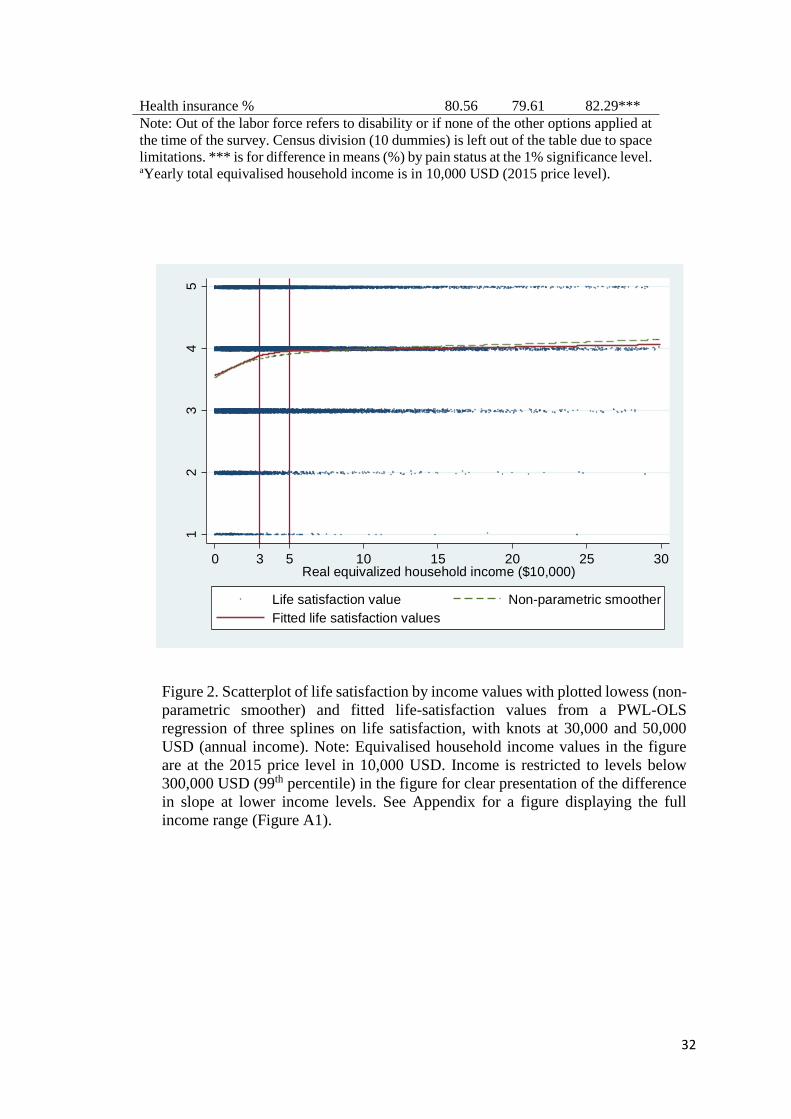
Figure 2. Scatterplot of life satisfaction by income values with plotted lowess (non-

parametric smoother) and fitted life-satisfaction values from a PWL-OLS

regression of three splines on life satisfaction, with knots at 30,000 and 50,000

USD (annual income). Note: Equivalised household income values in the figure

are at the 2015 price level in 10,000 USD. Income is restricted to levels below

300,000 USD (99th percentile) in the figure for clear presentation of the difference

in slope at lower income levels. See Appendix for a figure displaying the full

income range (Figure A1).

12

34

5

Life s

atisfa

ctio

n

0 3 5 10 15 20 25 30Real equivalized household income ($10,000)

Life satisfaction value Non-parametric smoother

Fitted life satisfaction values

Table 3: Point estimates and corresponding CVs by model estimator and functional form of income

Panel A OLS PWL-OLS FE PWL-FE OLS-IV

Coeff. CV

Coeff. CV

Coeff. CV

Coeff. CV

Coeff. CV

Pain -0.2123*** -0.2081*** -0.0563*** -0.0562*** -0.1999***

(0.0089) 910*** (0.0088) (0.0093) 1,040** (0.0093) (0.0103) 129***

Income 0.0064*** (115) 0.0015*** (422) 0.0426*** (42)

(0.0008) (0.0006) (0.0131)

Income

1. spline 0.0312*** 183*** 0.0017 NV

(0.0068) (40) (0.0073)

2. spline1 0.0598*** 95*** 0.0276*** 56***

(0.0062) (11) (0.0065) (16)

3. spline 0.0033*** 1,720*** 0.0005 NV

(0.0006) (301) (0.0005)

Panel B OLS FE OLS-IV

Coeff. CV

Coeff. CV

Coeff. CV

Pain -0.2089*** -0.0561*** -0.1922***

(0.0089) 2,377***

(0.0093) 3,983 (0.0107) 152**

ln(income) 0.0704*** (611) 0.0162*** (5,224) 0.2529*** (72)

(0.0049) (0.0053) (0.0753) N=64,205 person-years observations. N=58,588 in OLS-IV models. PWL: Piecewise linear. *p<0.10, ** p<0.05, *** p<0.01. Models include age, age squared, number of children in household, year dummies, dummies for comorbidities, marital status, census division, labor-force status, gender, education, race, Hispanic and health insurance. FE models include age, age squared, year dummies, dummies for comorbidities, marital status, labor-force status, children in household and health insurance as covariates in addition to pain and income. Knots are at income values 3 and 5 in PWL-OLS and PWL-FE models and the income variable is in 10,000 USD. CVs are reported in USD per day, 2015 price level and are calculated with coefficients from adjusted models. 1t-value for difference in slope between 1. and 2. segment in PWL-OLS model is -2.54. Results are unweighted. Weighted results are in Appendix. NV=no CV value as the income coefficient was not different from zero. Mean income in CV formula in Panel B=47,088. Standard errors (in parentheses) are clustered on individuals.

34

Table 4: Point estimates and corresponding CVs by model estimator and functional form of income

Men Women

Panel A OLS FE OLS-IV OLS FE OLS-IV

Pain -0.2129*** -0.0738*** -0.2058*** -0.2094*** -0.0450*** -0.1904***

(0.0140) (0.0149) (0.0151) (0.0115) (0.0120) (0.0138)

Income 0.0056*** 0.0021** 0.0204 0.0072*** 0.0010 0.0630***

(0.0010) (0.0009) (0.0172) (0.0011) (0.0007) (0.0192)

CV 1,035*** 950** 276 796*** 1,197 83***

(197) (431) (236) (126) (858) (28)

Panel B OLS FE OLS-IV OLS FE OLS-IV

Pain -0.2092*** -0.0734*** -0.2010*** -0.2068*** -0.0449*** -0.1827***

(0.0139) (0.0150) (0.0158) (0.0115) (0.0120) (0.0146)

ln(income) 0.0797*** 0.0244*** 0.1310 0.0635*** 0.0104 0.3562***

(0.0074) (0.0083) (0.1085) (0.0065) (0.0068) (0.1063)

CV 1,865*** 2,790 551 2,932** 8,792 81**

(608) (3,539) (930) (1,167) (27,396) (36) Men: N=26,876 person-years observations. N=24,342 in OLS-IV models. Women: N=37,329 person-years observations. N=34,246 in OLS-IV models.*p<0.10, ** p<0.05, *** p<0.01. Models include age, age squared, number of children in household, year dummies, dummies for comorbidities, marital status, census division, labor-force status, gender, education, race, Hispanic and health insurance. FE models include age, age squared, year dummies, dummies for comorbidities, marital status, labor force status, children in household and health insurance as covariates in addition to pain and income (income variable is in 10,000 USD). CVs are reported in USD per day, 2015 price level. Results are unweighted. Weighted results are in Appendix. Mean income in CV formula in Panel B=53,088 for men and 42,769 for women. Standard errors (in parentheses) are clustered on individuals.

35

Table 5: Point estimates and corresponding CVs by model estimator and functional form of income. 65 years and older

Panel A OLS PWL-OLS FE PWL-FE OLS-IV

Coeff. CV

Coeff. CV

Coeff. CV

Coeff. CV

Coeff. CV

Pain -0.1965*** -0.1943*** -0.0340*** -0.0339*** -0.1903***

(0.0113) 1,256*** (0.0112) (0.0123) 2,703 (0.0123) (0.0127) 116**

Income 0.0043*** (259) 0.0003 (5,224) 0.0451** (47)

(0.0008) (0.0007) (0.0180)

Income

1. spline 0.0286*** 186*** 0.0026 NV

(0.0089) (59) (0.0103)

2. spline 0.0431*** 123*** 0.0138 67

(0.0078) (23) (0.0084) (47)

3. spline 0.0019*** 2,776*** -0.0002 NV

(0.0007) (954) (0.0007)

Panel B OLS FE OLS-IV

Coeff. CV

Coeff. CV

Coeff. CV

Pain -0.1946*** -0.0339*** -0.1820***

(0.0112) 2,777**

(0.0123) NV (0.0123) 112**

ln(income) 0.0602*** (1,185) 0.0058 0.2735*** (63)

(0.0068) (0.0080) (0.1058) N=38,010 person-years observations. N=34,656 in OLS-IV models. PWL: Piecewise linear.*p<0.10, ** p<0.05, *** p<0.01. Models include age, age squared, number of children in household, year dummies, dummies for comorbidities, marital status, census division, labor force status, gender, education, race, Hispanic, and health insurance. FE models include age, age squared, year dummies, dummies for comorbidities, marital status, labor-force status, children in household and health insurance as covariates in addition to pain and income. Knots are at income values 3 and 5 in PWL-OLS and PWL-FE models and the income variable is in 10,000 USD. CVs are reported in USD per day, 2015 price level and are calculated with coefficients from adjusted models. Results are unweighted. Weighted results are in Appendix. NV=no CV value as the income coefficient was not different from zero. Mean income in CV formula in Panel B= 47,097. Standard errors (in parentheses) are clustered on individuals.

Table 6 CV estimates by pain severity

Panel A: linear income (1) (2) (3)

OLS FE OLS-IV

Pain

Mild 434*** 639** 65***

(72) (639) (23)

Moderate 1,008*** 1,023** 144***

(128) (428) (47)

Severe 1,547*** 2,500** 225***

(203) (996) (75)

Panel B: ln(income) (1) (2) (3)

OLS FE OLS-IV

Pain

Mild 409*** 948 63**

(106) (1,067) (27)

Moderate 3,510*** 3,766 180**

(1,029) (5,059) (88)

Severe 20,658** 543,290 357

(9,682) (1,612,647) (219)

*p<0.10, ** p<0.05, *** p<0.01

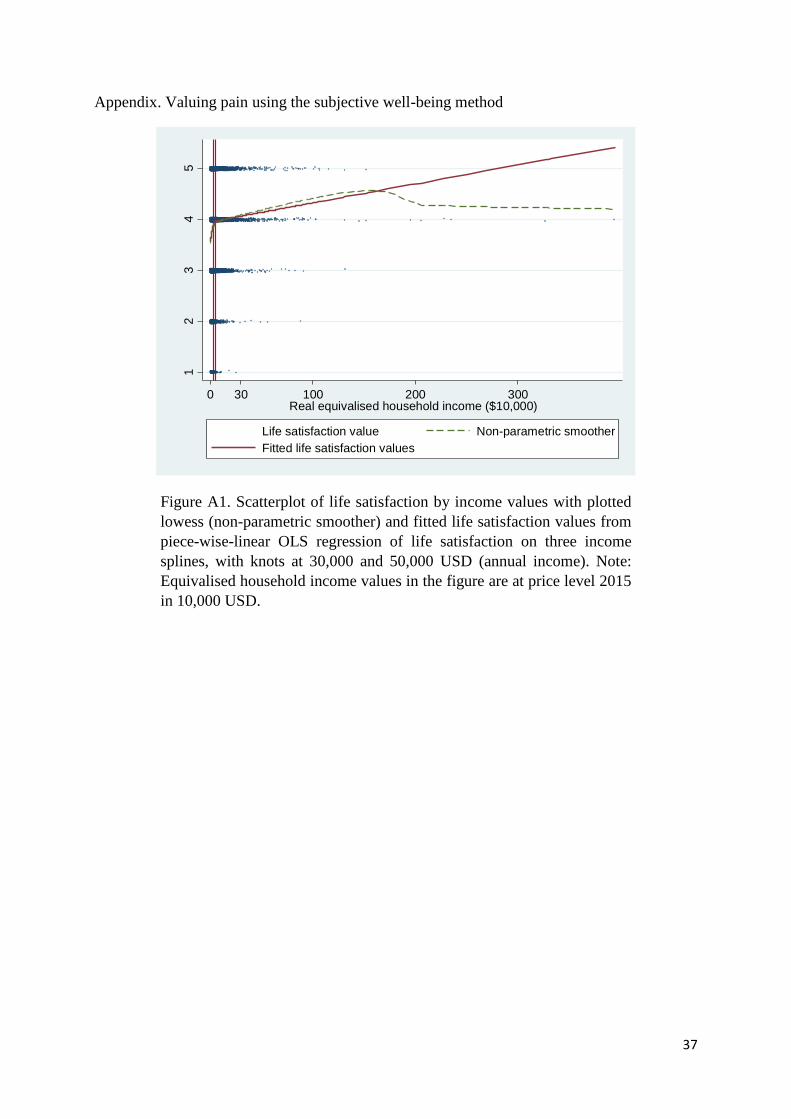
37

Appendix. Valuing pain using the subjective well-being method

Figure A1. Scatterplot of life satisfaction by income values with plotted

lowess (non-parametric smoother) and fitted life satisfaction values from

piece-wise-linear OLS regression of life satisfaction on three income

splines, with knots at 30,000 and 50,000 USD (annual income). Note:

Equivalised household income values in the figure are at price level 2015

in 10,000 USD.

12

34

5

Life s

atisfa

ctio

n

0 30 100 200 300Real equivalised household income ($10,000)

Life satisfaction value Non-parametric smoother

Fitted life satisfaction values

38

Figure A2. The connected points on the figure are predicted life-

satisfaction values (margins) up to income of 300,000 USD from a

regression of life satisfaction on 30 income dummies with income rounded

to nearest integer.

Figure A3. Same as Figure A2 but here over the full income range (highest

value is 3,950,000 USD). The figure displays the volatility in the life

satisfaction predictions at higher income levels. Note income above

300,000 USD at price level 2015 is top 1% of the income distribution.

3.6

3.8

44

.24

.4

Lin

ea

r P

redic

tion

0 10 20 30Real equivalised household income ($10,000)

Predicted life satisfaction with 95% CIs

33

.54

4.5

5

Lin

ea

r P

redic

tion

0 100 200 300 400Real equivalised household income ($10,000)

Predicted life satisfaction

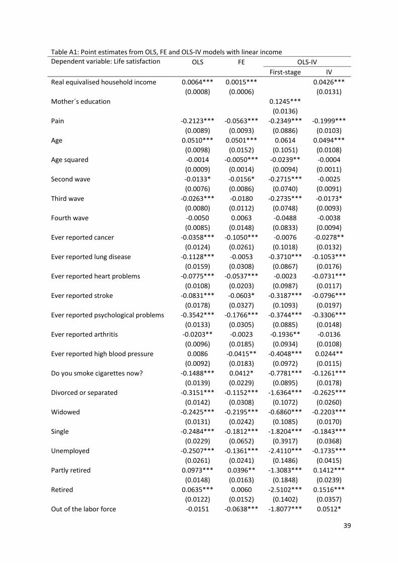
39

Table A1: Point estimates from OLS, FE and OLS-IV models with linear income

Dependent variable: Life satisfaction OLS FE OLS-IV

First-stage IV

Real equivalised household income 0.0064*** 0.0015*** 0.0426***

(0.0008) (0.0006) (0.0131)

Mother´s education 0.1245***

(0.0136) Pain -0.2123*** -0.0563*** -0.2349*** -0.1999***

(0.0089) (0.0093) (0.0886) (0.0103)

Age 0.0510*** 0.0501*** 0.0614 0.0494***

(0.0098) (0.0152) (0.1051) (0.0108)

Age squared -0.0014 -0.0050*** -0.0239** -0.0004

(0.0009) (0.0014) (0.0094) (0.0011)

Second wave -0.0133* -0.0156* -0.2715*** -0.0025

(0.0076) (0.0086) (0.0740) (0.0091)

Third wave -0.0263*** -0.0180 -0.2735*** -0.0173*

(0.0080) (0.0112) (0.0748) (0.0093)

Fourth wave -0.0050 0.0063 -0.0488 -0.0038

(0.0085) (0.0148) (0.0833) (0.0094)

Ever reported cancer -0.0358*** -0.1050*** -0.0076 -0.0278**

(0.0124) (0.0261) (0.1018) (0.0132)

Ever reported lung disease -0.1128*** -0.0053 -0.3710*** -0.1053***

(0.0159) (0.0308) (0.0867) (0.0176)

Ever reported heart problems -0.0775*** -0.0537*** -0.0023 -0.0731***

(0.0108) (0.0203) (0.0987) (0.0117)

Ever reported stroke -0.0831*** -0.0603* -0.3187*** -0.0796***

(0.0178) (0.0327) (0.1093) (0.0197)

Ever reported psychological problems -0.3542*** -0.1766*** -0.3744*** -0.3306***

(0.0133) (0.0305) (0.0885) (0.0148)

Ever reported arthritis -0.0203** -0.0023 -0.1936** -0.0136

(0.0096) (0.0185) (0.0934) (0.0108)

Ever reported high blood pressure 0.0086 -0.0415** -0.4048*** 0.0244**

(0.0092) (0.0183) (0.0972) (0.0115)

Do you smoke cigarettes now? -0.1488*** 0.0412* -0.7781*** -0.1261***

(0.0139) (0.0229) (0.0895) (0.0178)

Divorced or separated -0.3151*** -0.1152*** -1.6364*** -0.2625***

(0.0142) (0.0308) (0.1072) (0.0260)

Widowed -0.2425*** -0.2195*** -0.6860*** -0.2203***

(0.0131) (0.0242) (0.1085) (0.0170)

Single -0.2484*** -0.1812*** -1.8204*** -0.1843***

(0.0229) (0.0652) (0.3917) (0.0368)

Unemployed -0.2507*** -0.1361*** -2.4110*** -0.1735***

(0.0261) (0.0241) (0.1486) (0.0415)

Partly retired 0.0973*** 0.0396** -1.3083*** 0.1412***

(0.0148) (0.0163) (0.1848) (0.0239)

Retired 0.0635*** 0.0060 -2.5102*** 0.1516***

(0.0122) (0.0152) (0.1402) (0.0357)

Out of the labor force -0.0151 -0.0638*** -1.8077*** 0.0512*

40

(0.0188) (0.0223) (0.1523) (0.0310)

Number of resident children -0.0155** -0.0004 -0.8023*** 0.0085

(0.0068) (0.0106) (0.0525) (0.0129)

Female 0.0631*** -0.2982*** 0.0727***

(0.0096) (0.0958) (0.0112)

GED and high school graduate -0.0087 0.2146*** -0.0171

(0.0145) (0.0704) (0.0170)

Some college -0.0513*** 1.0231*** -0.1000***

(0.0155) (0.0904) (0.0245)

College and above -0.0071 3.8386*** -0.1612***

(0.0161) (0.1394) (0.0580)

Black/African American -0.0589*** -1.3026*** -0.0085

(0.0134) (0.0817) (0.0237)

Other 0.0222 -0.4982*** 0.0584**

(0.0208) (0.1803) (0.0246)

Hispanic==1 -0.0220 -1.2094*** 0.0410

(0.0184) (0.1451) (0.0301)

Health insurance 0.0795*** 0.0601*** 0.1828* 0.0763***

(0.0121) (0.0140) (0.1102) (0.0132)

Constant 3.7789*** 3.8713*** 7.0925*** 3.4849***

(0.0359) (0.0457) (0.4303) (0.1163)

Observations 64,205 64,205 58,588 58,588

Adjusted R-squared 0.1259 0.0096 0.1407 0.0368

F-statistic of excluding instrument 83.95

Anderson-Rubin F-test (p-value) 0.0008

Standard errors in parentheses. * p<0.10, ** p<0.05, *** p<0.01. Reference groups are married or partnered, employed, less than high school and white.

41

Table A2: point estimates from OLS, FE and OLS-IV models with ln(income)

Dependent variable: Life satisfaction OLS FE OLS-IV

First-stage IV

Real equivalised household income(ln) 0.0704*** 0.0162*** 0.2529***

(0.0049) (0.0053) (0.0753)

Mother´s education 0.0210***

(0.0017) Pain -0.2089*** -0.0561*** -0.0702*** -0.1922***

(0.0089) (0.0093) (0.0092) (0.0107)

Age 0.0487*** 0.0500*** 0.0358*** 0.0429***

(0.0097) (0.0152) (0.0106) (0.0105)

Age squared -0.0011 -0.0051*** -0.0052*** -0.0001

(0.0009) (0.0014) (0.0010) (0.0011)

Second wave -0.0135* -0.0153* -0.0247*** -0.0079

(0.0076) (0.0086) (0.0076) (0.0082)

Third wave -0.0245*** -0.0172 -0.0485*** -0.0167*

(0.0079) (0.0112) (0.0078) (0.0089)

Fourth wave -0.0033 0.0072 -0.0286*** 0.0013

(0.0085) (0.0148) (0.0087) (0.0090)

Ever reported cancer -0.0380*** -0.1052*** 0.0303** -0.0358***

(0.0124) (0.0261) (0.0126) (0.0131)

Ever reported lung disease -0.1083*** -0.0053 -0.0916*** -0.0979***

(0.0159) (0.0308) (0.0158) (0.0183)

Ever reported heart problems -0.0764*** -0.0534*** -0.0186* -0.0685***

(0.0108) (0.0203) (0.0111) (0.0115)

Ever reported stroke -0.0784*** -0.0596* -0.0978*** -0.0684***

(0.0178) (0.0327) (0.0168) (0.0205)

Ever reported psychological problems -0.3510*** -0.1760*** -0.0798*** -0.3264***

(0.0132) (0.0305) (0.0134) (0.0151)

Ever reported arthritis -0.0213** -0.0023 -0.0030 -0.0211**

(0.0095) (0.0185) (0.0106) (0.0101)

Ever reported high blood pressure 0.0096 -0.0415** -0.0524*** 0.0204*

(0.0092) (0.0183) (0.0103) (0.0106)

Do you smoke cigarettes now? -0.1421*** 0.0413* -0.1618*** -0.1184***

(0.0138) (0.0229) (0.0151) (0.0189)

Divorced or separated -0.2887*** -0.1101*** -0.5252*** -0.1994***

(0.0143) (0.0308) (0.0161) (0.0422)

Widowed -0.2235*** -0.2162*** -0.3312*** -0.1658***

(0.0132) (0.0242) (0.0137) (0.0286)

Single -0.2149*** -0.1757*** -0.6358*** -0.1011*

(0.0229) (0.0652) (0.0288) (0.0532)

Unemployed -0.2253*** -0.1340*** -0.5725*** -0.1315***

(0.0261) (0.0241) (0.0305) (0.0510)

Partly retired 0.1105*** 0.0414** -0.3085*** 0.1635***

(0.0147) (0.0163) (0.0175) (0.0279)

Retired 0.0885*** 0.0092 -0.5728*** 0.1895***

(0.0124) (0.0152) (0.0141) (0.0452)

Out of the labor force 0.0151 -0.0605*** -0.5720*** 0.1188**

42

(0.0189) (0.0223) (0.0230) (0.0474)

Number of resident children -0.0043 0.0015 -0.2234*** 0.0308*

(0.0068) (0.0106) (0.0077) (0.0185)

Female 0.0647*** -0.0478*** 0.0721***

(0.0096) (0.0106) (0.0107)

GED and high school graduate -0.0272* 0.2661*** -0.0753***

(0.0146) (0.0148) (0.0278)

Some college -0.0775*** 0.4336*** -0.1661***

(0.0157) (0.0166) (0.0406)

College and above -0.0409** 0.7874*** -0.1967***

(0.0164) (0.0182) (0.0669)

Black/African American -0.0427*** -0.3346*** 0.0206

(0.0135) (0.0150) (0.0306)

Other 0.0282 -0.1089*** 0.0647***

(0.0208) (0.0256) (0.0246)

Hispanic==1 -0.0001 -0.3913*** 0.0884**

(0.0184) (0.0213) (0.0408)

Health insurance 0.0723*** 0.0593*** 0.1190*** 0.0540***

(0.0120) (0.0140) (0.0153) (0.0156)

Constant 3.7258*** 3.8572*** 1.3094*** 3.4560***

(0.0361) (0.0462) (0.0440) (0.1202)

Observations 64,205 64,205 58,588 58,588

Adjusted R-squared 0.1277 0.0097 0.3731 0.1003

F-statistic of excluding instrument 160.07

Anderson-Rubin F-test (p-value) 0.0008

Standard errors in parentheses. * p<0.10, ** p<0.05, *** p<0.01. Reference groups are married or partnered, employed, less than high school and white.

43

Table A3: CV estimates from unadjusted and adjusted models

Panel A OLS FE

Unadjusted Adjusted Unadjusted Adjusted

Pain -0.3113*** -0.2123*** -0.0575*** -0.0563***

(0.0092) (0.0089) (0.0093) (0.0093)

Income 0.0091*** 0.0064*** 0.0017*** 0.0015***

(0.0009) (0.0008) (0.0006) (0.0006)

CV 910*** 1,040**

(115) (422)

Panel B OLS FE

Unadjusted Adjusted Unadjusted Adjusted

Pain -0.2926*** -0.2089*** -0.0570*** -0.0561***

(0.0091) (0.0089) (0.0094) (0.0093)

ln(income) 0.1057*** 0.0704*** 0.0236*** 0.0162***

(0.0043) (0.0049) (0.0052) (0.0053)

CV 2,377*** 3,983

(611) (5,224)

*p<0.10, ** p<0.05, *** p<0.01. Unadjusted models include pain and real equivalized household income in panel A and ln (real equivalized household income) in panel B. Adjusted models also include age, age squared, number of children in household, year dummies, dummies for comorbidities, marital status, census division, labor-force status, gender, education, race, Hispanic and health insurance. FE models include age, age squared, year dummies, dummies for comorbidities, marital status, labor force status, children in household and health insurance as covariates in addition to pain and income. CVs are reported in USD per day, 2015 price level. Unweighted results. Standard errors (in parentheses) are clustered on individuals.

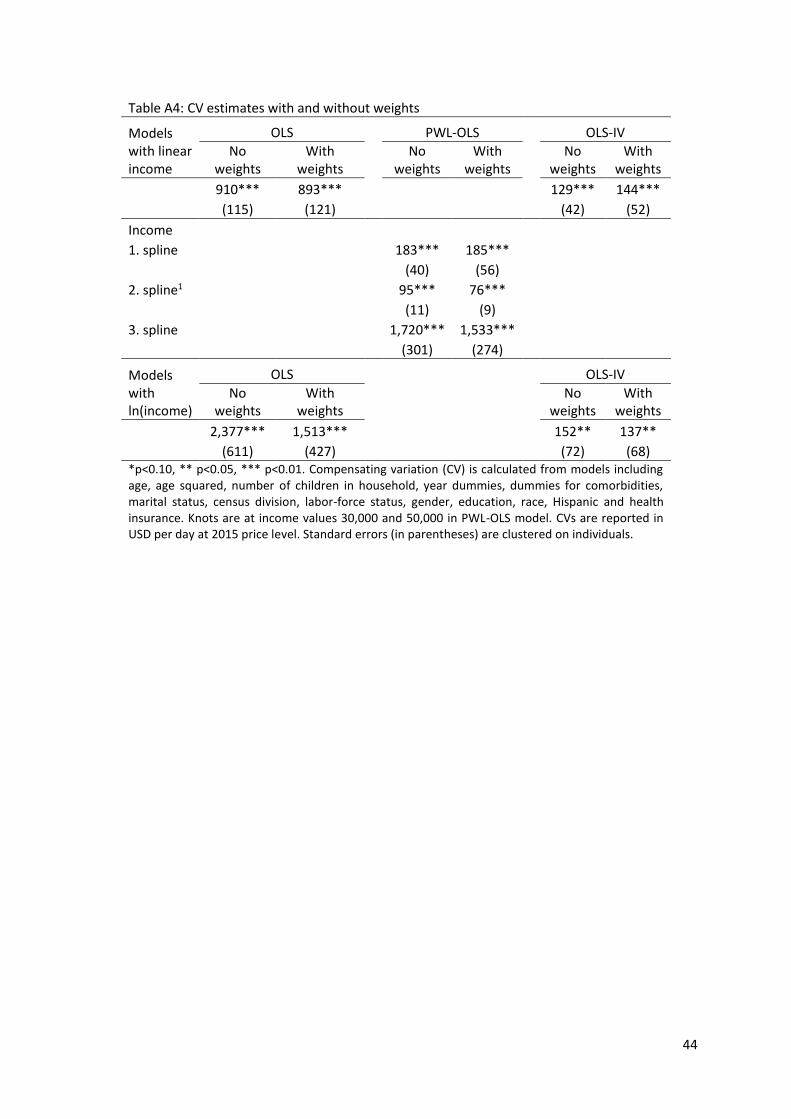
44

Table A4: CV estimates with and without weights

Models with linear income

OLS PWL-OLS OLS-IV

No weights

With weights

No weights

With weights

No weights

With weights

910*** 893*** 129*** 144***

(115) (121) (42) (52)

Income

1. spline 183*** 185***

(40) (56)

2. spline1 95*** 76***

(11) (9)

3. spline 1,720*** 1,533***

(301) (274)

Models with ln(income)

OLS OLS-IV

No weights

With weights

No weights

With weights

2,377*** 1,513***

152** 137**

(611) (427)

(72) (68) *p<0.10, ** p<0.05, *** p<0.01. Compensating variation (CV) is calculated from models including age, age squared, number of children in household, year dummies, dummies for comorbidities, marital status, census division, labor-force status, gender, education, race, Hispanic and health insurance. Knots are at income values 30,000 and 50,000 in PWL-OLS model. CVs are reported in USD per day at 2015 price level. Standard errors (in parentheses) are clustered on individuals.