Valuation - New York Universitypeople.stern.nyu.edu/adamodar/pdfiles/country/Germanyval04.pdf ·...
227
Aswath Damodaran 1 Valuation Aswath Damodaran http://www.damodaran.com Details on valuations in this presentation: http://pages.stern. nyu . edu/~adamodar/New_Home_Page/country . htm
Transcript of Valuation - New York Universitypeople.stern.nyu.edu/adamodar/pdfiles/country/Germanyval04.pdf ·...

Aswath Damodaran 1
ValuationAswath Damodaran
http://www.damodaran.com
Details on valuations in this presentation:http://pages.stern.nyu.edu/~adamodar/New_Home_Page/country.htm

Aswath Damodaran 2
Some Initial Thoughts
" One hundred thousand lemmings cannot be wrong"Graffiti

Aswath Damodaran 3
Misconceptions about Valuation
Myth 1: A valuation is an objective search for “true” value• Truth 1.1: All valuations are biased. The only questions are how much and in
which direction.• Truth 1.2: The direction and magnitude of the bias in your valuation is directly
proportional to who pays you and how much you are paid. Myth 2.: A good valuation provides a precise estimate of value
• Truth 2.1: There are no precise valuations• Truth 2.2: The payoff to valuation is greatest when valuation is least precise.
Myth 3: . The more quantitative a model, the better the valuation• Truth 3.1: One’s understanding of a valuation model is inversely proportional to
the number of inputs required for the model.• Truth 3.2: Simpler valuation models do much better than complex ones.
Aswath Damodaran 4
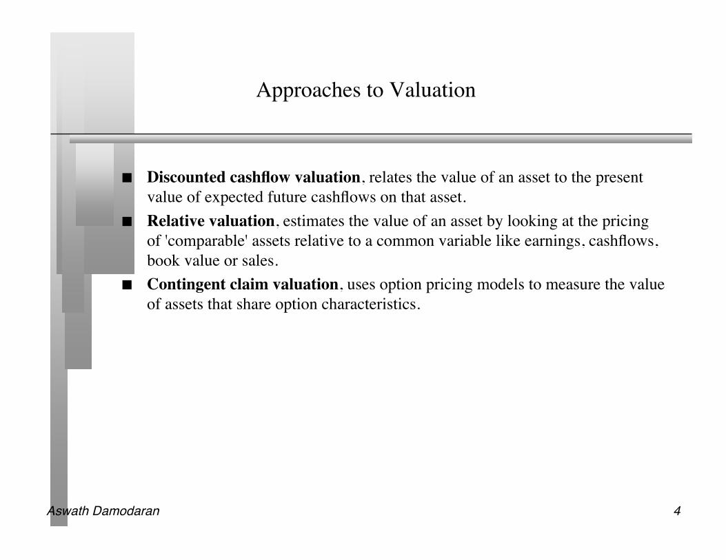
Approaches to Valuation
Discounted cashflow valuation, relates the value of an asset to the presentvalue of expected future cashflows on that asset.
Relative valuation, estimates the value of an asset by looking at the pricingof 'comparable' assets relative to a common variable like earnings, cashflows,book value or sales.
Contingent claim valuation, uses option pricing models to measure the valueof assets that share option characteristics.
Aswath Damodaran 5
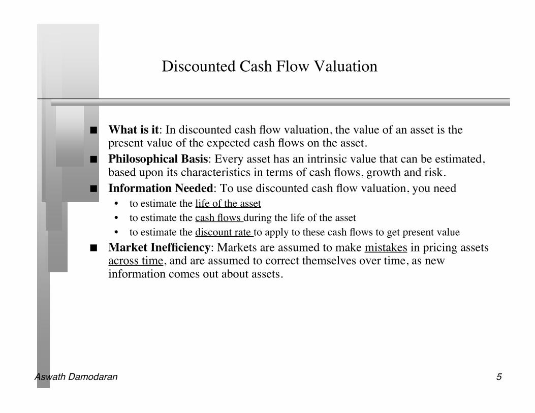
Discounted Cash Flow Valuation
What is it: In discounted cash flow valuation, the value of an asset is thepresent value of the expected cash flows on the asset.
Philosophical Basis: Every asset has an intrinsic value that can be estimated,based upon its characteristics in terms of cash flows, growth and risk.
Information Needed: To use discounted cash flow valuation, you need• to estimate the life of the asset• to estimate the cash flows during the life of the asset• to estimate the discount rate to apply to these cash flows to get present value
Market Inefficiency: Markets are assumed to make mistakes in pricing assetsacross time, and are assumed to correct themselves over time, as newinformation comes out about assets.

Aswath Damodaran 6
Equity Valuation
Assets Liabilities
Assets in Place Debt
Equity
Discount rate reflects only the cost of raising equity financing
Growth Assets
Figure 5.5: Equity Valuation
Cash flows considered are cashflows from assets, after debt payments and after making reinvestments needed for future growth
Present value is value of just the equity claims on the firm

Aswath Damodaran 7
Firm Valuation
Assets Liabilities
Assets in Place Debt
Equity
Discount rate reflects the cost of raising both debt and equity financing, in proportion to their use
Growth Assets
Figure 5.6: Firm Valuation
Cash flows considered are cashflows from assets, prior to any debt paymentsbut after firm has reinvested to create growth assets
Present value is value of the entire firm, and reflects the value of all claims on the firm.

Aswath Damodaran 8
Valuation with Infinite Life
Cash flowsFirm: Pre-debt cash flowEquity: After debt cash flows
Expected GrowthFirm: Growth in Operating EarningsEquity: Growth in Net Income/EPS
CF1 CF2 CF3 CF4 CF5
Forever
Firm is in stable growth:Grows at constant rateforever
Terminal Value
CFn.........
Discount RateFirm:Cost of Capital
Equity: Cost of Equity
ValueFirm: Value of Firm
Equity: Value of Equity
DISCOUNTED CASHFLOW VALUATION
Length of Period of High Growth

Aswath Damodaran 9
Cashflow to FirmEBIT (1-t)- (Cap Ex - Depr)- Change in WC= FCFF
Expected GrowthReinvestment Rate* Return on Capital
FCFF1 FCFF2 FCFF3 FCFF4 FCFF5
Forever
Firm is in stable growth:Grows at constant rateforever
Terminal Value= FCFF n+1/(r-gn)
FCFFn.........
Cost of Equity Cost of Debt(Riskfree Rate+ Default Spread) (1-t)
WeightsBased on Market Value
Discount at WACC= Cost of Equity (Equity/(Debt + Equity)) + Cost of Debt (Debt/(Debt+ Equity))
Value of Operating Assets+ Cash & Non-op Assets= Value of Firm- Value of Debt= Value of Equity
Riskfree Rate :- No default risk- No reinvestment risk- In same currency andin same terms (real or nominal as cash flows
+Beta- Measures market risk X
Risk Premium- Premium for averagerisk investment
Type of Business
Operating Leverage
FinancialLeverage
Base EquityPremium
Country RiskPremium
DISCOUNTED CASHFLOW VALUATION

Aswath Damodaran 10
Current Cashflow to FirmEBIT(1-t) : 2,227- Nt CpX 687 - Chg WC 583= FCFF ! 958Reinvestment Rate=(687+583)/2227
= 57%
Expected Growth in EBIT (1-t).57*.0917=.05235.23%
Stable Growthg = 2%; Beta = 1.00;Country Premium= 1.5%Cost of capital = 7.15% ROC= 7.15%; Tax rate=37%Reinvestment Rate=g/ROC
=2/ 7.15= 27.97%
Terminal Value5= 2225/(.0715-.02) = 43,205
Cost of Equity 8.52%
Cost of Debt(3.95%+1.50%)(1-.4021)= 3.26%
WeightsE = 80.15% D = 19.85%
Discount at $ Cost of Capital (WACC) = 8.52% (.8015) + 3.26% (0.1985) = 7.47%
Op. Assets! 34,631+ Cash: 4,123- Debt 5,597- Non-Debt 7,517=Equity 25,640
Value/Sh ! 38.07
Riskfree Rate:Euro Riskfree Rate= 3.95%
+Beta 1.14 X
Mature market premium 3.83 %
Unlevered Beta for Sectors: 0.99
Firm’s D/ERatio: 24.77%
BMW: Status Quo (Euros) Reinvestment Rate 57%
Return on Capital9.17%
Term Yr 3089 - 864= 2225
+ Lambda0.08
XEmerg Market Equity Risk Premium2.50%
On Sept 23, 2004BMW Common = 33.50 Eu
Euro Cashflows
Year 1 2 3 4 5EBIT (1-t) ! 2,344 ! 2,467 ! 2,596 ! 2,731 ! 2,874Reinvestment ! 1,336 ! 1,406 ! 1,479 ! 1,557 ! 1,638FCFF ! 1,008 ! 1,061 ! 1,116 ! 1,174 ! 1,236
g=2%Tax rate changes

Aswath Damodaran 11
FCFF1 FCFF2 FCFF3 FCFF4 FCFF5
Forever
Terminal Value= FCFF n+1/(r-gn)
FCFFn.........
Cost of Equity Cost of Debt(Riskfree Rate+ Default Spread) (1-t)
WeightsBased on Market Value
Discount at WACC= Cost of Equity (Equity/(Debt + Equity)) + Cost of Debt (Debt/(Debt+ Equity))
Value of Operating Assets+ Cash & Non-op Assets= Value of Firm- Value of Debt= Value of Equity- Equity Options= Value of Equity in Stock
Riskfree Rate :- No default risk- No reinvestment risk- In same currency andin same terms (real or nominal as cash flows
+Beta- Measures market risk X
Risk Premium- Premium for averagerisk investment
Type of Business
Operating Leverage
FinancialLeverage
Base EquityPremium
Country RiskPremium
CurrentRevenue
CurrentOperatingMargin
Reinvestment
Sales TurnoverRatio
CompetitiveAdvantages
Revenue Growth
Expected Operating Margin
Stable Growth
StableRevenueGrowth
StableOperatingMargin
StableReinvestment
Discounted Cash Flow Valuation: High Growth with Negative Earnings
EBIT
Tax Rate- NOLs
FCFF = Revenue* Op Margin (1-t) - Reinvestment

Aswath Damodaran 12
Forever
Terminal Value= 1881/(.0961-.06)=52,148
Cost of Equity12.90%
Cost of Debt6.5%+1.5%=8.0%Tax rate = 0% -> 35%
WeightsDebt= 1.2% -> 15%
Value of Op Assets $ 14,910+ Cash $ 26= Value of Firm $14,936- Value of Debt $ 349= Value of Equity $14,587- Equity Options $ 2,892Value per share $ 34.32
Riskfree Rate :T. Bond rate = 6.5%
+Beta1.60 -> 1.00 X
Risk Premium4%
Internet/Retail
Operating Leverage
Current D/E: 1.21%
Base EquityPremium
Country RiskPremium
CurrentRevenue$ 1,117
CurrentMargin:-36.71%
Reinvestment:Cap ex includes acquisitionsWorking capital is 3% of revenues
Sales TurnoverRatio: 3.00
CompetitiveAdvantages
Revenue Growth:42%
Expected Margin: -> 10.00%
Stable Growth
StableRevenueGrowth: 6%
StableOperatingMargin: 10.00%
Stable ROC=20%Reinvest 30% of EBIT(1-t)
EBIT-410m
NOL:500 m
$41,346
10.00%
35.00%
$2,688
$ 807
$1,881
Term. Year
2 431 5 6 8 9 107
Cost of Equity 12.90% 12.90% 12.90% 12.90% 12.90% 12.42% 12.30% 12.10% 11.70% 10.50%
Cost of Debt 8.00% 8.00% 8.00% 8.00% 8.00% 7.80% 7.75% 7.67% 7.50% 7.00%
AT cost of debt 8.00% 8.00% 8.00% 6.71% 5.20% 5.07% 5.04% 4.98% 4.88% 4.55%
Cost of Capital 12.84% 12.84% 12.84% 12.83% 12.81% 12.13% 11.96% 11.69% 11.15% 9.61%
Revenues $2,793 5,585 9,774 14,661 19,059 23,862 28,729 33,211 36,798 39,006
EBIT -$373 -$94 $407 $1,038 $1,628 $2,212 $2,768 $3,261 $3,646 $3,883
EBIT (1-t) -$373 -$94 $407 $871 $1,058 $1,438 $1,799 $2,119 $2,370 $2,524
- Reinvestment $559 $931 $1,396 $1,629 $1,466 $1,601 $1,623 $1,494 $1,196 $736
FCFF -$931 -$1,024 -$989 -$758 -$408 -$163 $177 $625 $1,174 $1,788
Amazon.comJanuary 2000Stock Price = $ 84

Aswath Damodaran 13
I. Discount Rates:Cost of Equity
Cost of Equity = Riskfree Rate + Beta * (Risk Premium)
Has to be in the samecurrency as cash flows, and defined in same terms(real or nominal) as thecash flows
Preferably, a bottom-up beta,based upon other firms in thebusiness, and firm’s own financialleverage
Historical Premium1. Mature Equity Market Premium:Average premium earned bystocks over T.Bonds in U.S.2. Country risk premium =
Country Default Spread* ( !Equity/!Country bond)
Implied PremiumBased on how equitymarket is priced todayand a simple valuationmodel
or

Aswath Damodaran 14
A Simple Test
You are valuing BMW in Euros for a US institutional investor and areattempting to estimate a risk free rate to use in the analysis. The risk free ratethat you should use is
The interest rate on a US $ denominated treasury bond (4.25%) The interest rate on a Euro-denominated bond issued by the German
government (3.95%) The lowest interest rate on a 10-year Euro-denominated bond issued by any
European government (3.95%) The lowest interest rate on a 10-year bond issued by a European government
(Swiss bond: 2.62%)

Aswath Damodaran 15
Everyone uses historical premiums, but..
The historical risk premium is easiest to estimate in the United States, becausethere is unbroken market data going back to 1870.
Arithmetic average Geometric AverageStocks - Stocks - Stocks - Stocks -
Historical Period T.Bills T.Bonds T.Bills T.Bonds1928-2003 7.92% 6.54% 5.99% 4.82%1963-2003 6.09% 4.70% 4.85% 3.82%1993-2003 8.43% 4.87% 6.68% 3.57% It is difficult to get enough historical data to estimate risk premiums in
other countries.

Aswath Damodaran 16
Risk Premium for a Mature Market? Broadening the sample..

Aswath Damodaran 17
An Alternative to Historical Risk Premiums: Implied EquityPremium for the S&P 500: January 1, 2004
We can use the information in stock prices to back out how risk averse the market is and how muchof a risk premium it is demanding.
If you pay the current level of the index, you can expect to make a return of 7.94% on stocks (whichis obtained by solving for r in the following equation)
Implied Equity risk premium = Expected return on stocks - Treasury bond rate = 7.94% - 4.25% =3.69%
January 1, 2004S&P 500 is at 1111.91
In 2003, dividends & stock buybacks were 2.81% of the index, generating 31.29 in cashflows
Analysts expect earnings to grow 9.5% a year for the next 5 years as the economy comes out of a recession.
After year 5, we will assume that earnings on the index will grow at 4.25%, the same rate as the entire economy
34.26 37.52 41.08 44.98 49.26
!
1111.91=34.26
(1+ r)+37.52
(1+ r)2
+41.08
(1+ r)3
+44.98
(1+ r)4
+49.26
(1+ r)5
+49.26(1.0425)
(r " .0425)(1+ r)5

Aswath Damodaran 18
Implied Premiums in the US

Aswath Damodaran 19
Choosing an Equity Risk Premium
Historical Risk Premium: When you use the historical risk premium, you areassuming that premiums will revert back to a historical norm and that the timeperiod that you are using is the right norm. You are also more likely to findstocks to be overvalued than undervalued (Why?)
Current Implied Equity Risk premium: You are assuming that the market iscorrect in the aggregate but makes mistakes on individual stocks. If you arerequired to be market neutral, this is the premium you should use. (Whattypes of valuations require market neutrality?)
Average Implied Equity Risk premium: The average implied equity riskpremium between 1960-2003 in the United States is about 4%. You areassuming that the market is correct on average but not necessarily at a point intime.

Aswath Damodaran 20
Implied Equity Risk Premium for Germany: September 23,2004
We can use the information in stock prices to back out how risk averse the market is and how muchof a risk premium it is demanding.
If you pay the current level of the index, you can expect to make a return of 7.94% on stocks (whichis obtained by solving for r in the following equation)
Implied Equity risk premium = Expected return on stocks - Treasury bond rate = 7.78% - 3.95% =3.83%
!
3905.65=116.13
(1+ r)+129.32
(1+ r)2
+144.01
(1+ r)3
+160.37
(1+ r)4
+178.59
(1+ r)5
+178.59(1.0395)
(r " .0425)(1+ r)5
Buy the index for 3905.65
Dividends and stock buybacks were 2.67% of the index last yearSource: Bloomberg
Analysts are estimating an expected growth rate of 11.36% in earningsover the next 5 years for stocks in the DAX (Source: IBES)
116.13 129.32 144.01 160.37 178.59
Expected dividends and stock buybacks over next 5 years
Assumed to growat 3.95% a yearforever after year 5

Aswath Damodaran 21
Opportunities and Threats: The Allure of Asia and theRisk…
Country Rating Typical Default SpreadChina A2 90Hong Kong A1 80India Baa2 130Indonesia B2 550Malaysia A3 95Pakistan B2 550Singapore Aaa 0Taiwan Aa3 70Thailand Baa1 120Vietnam B1 450Vietnam B1 450
Aswath Damodaran 22
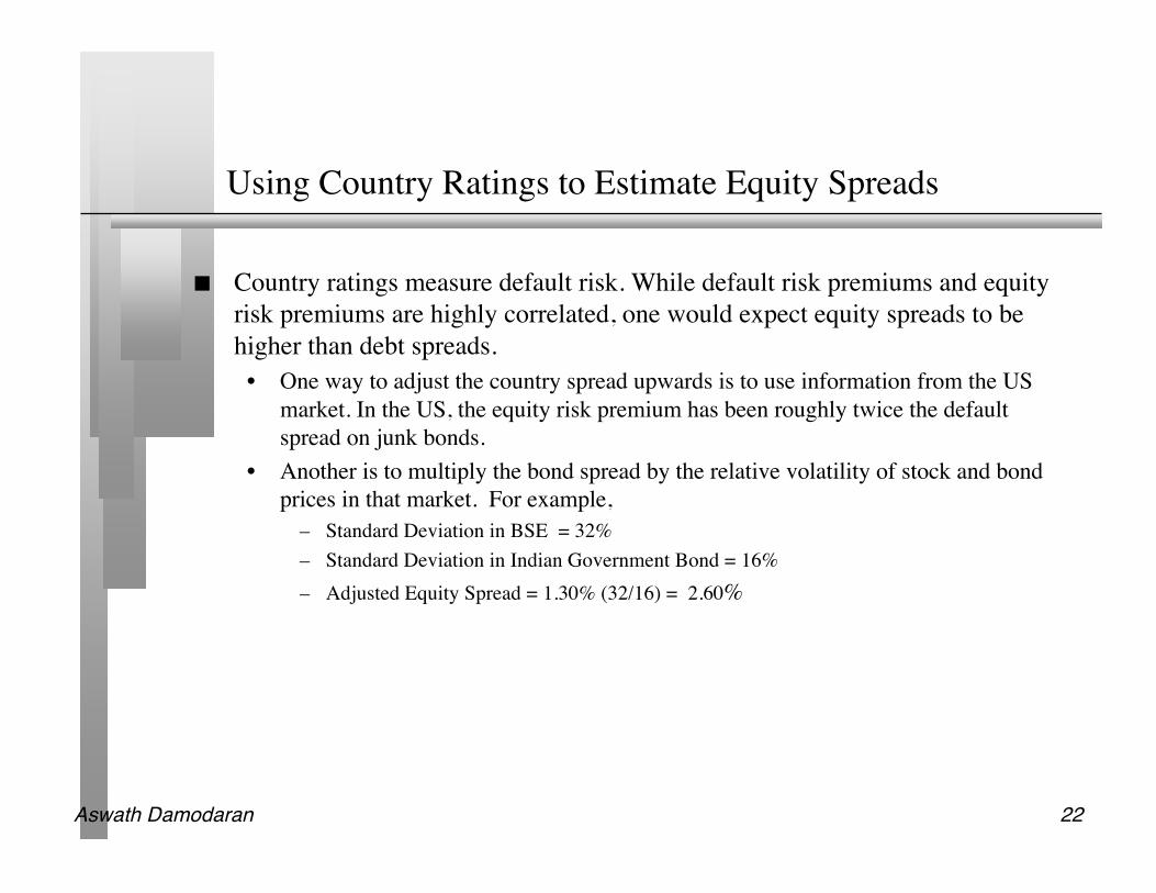
Using Country Ratings to Estimate Equity Spreads
Country ratings measure default risk. While default risk premiums and equityrisk premiums are highly correlated, one would expect equity spreads to behigher than debt spreads.
• One way to adjust the country spread upwards is to use information from the USmarket. In the US, the equity risk premium has been roughly twice the defaultspread on junk bonds.
• Another is to multiply the bond spread by the relative volatility of stock and bondprices in that market. For example,
– Standard Deviation in BSE = 32%– Standard Deviation in Indian Government Bond = 16%– Adjusted Equity Spread = 1.30% (32/16) = 2.60%

Aswath Damodaran 23
Equity Risk Premiums in Asia
Country Rating Typical Default Spread Relative Equity Market volatility Equity Risk Premium
China A2 90 2.25 2.03%
Hong Kong A1 80 1.8 1.44%
India Baa2 130 2 2.60%
Indonesia B2 550 1.8 9.90%
Malaysia A3 95 2.5 2.38%
Pakistan B2 550 1.75 9.63%
Singapore Aaa 0 2.2 0.00%
Taiwan Aa3 70 2.5 1.75%
Thailand Baa1 120 2.2 2.64%
Vietnam B1 450 1.6 7.20%
2.50%Weighted average risk premium =
Aswath Damodaran 24
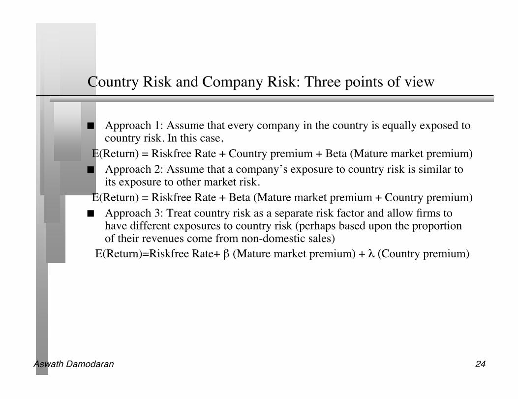
Country Risk and Company Risk: Three points of view
Approach 1: Assume that every company in the country is equally exposed tocountry risk. In this case,
E(Return) = Riskfree Rate + Country premium + Beta (Mature market premium) Approach 2: Assume that a company’s exposure to country risk is similar to
its exposure to other market risk.E(Return) = Riskfree Rate + Beta (Mature market premium + Country premium) Approach 3: Treat country risk as a separate risk factor and allow firms to
have different exposures to country risk (perhaps based upon the proportionof their revenues come from non-domestic sales)
E(Return)=Riskfree Rate+ β (Mature market premium) + λ (Country premium)
Aswath Damodaran 25
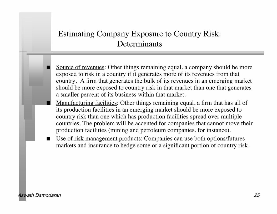
Estimating Company Exposure to Country Risk:Determinants
Source of revenues: Other things remaining equal, a company should be moreexposed to risk in a country if it generates more of its revenues from thatcountry. A firm that generates the bulk of its revenues in an emerging marketshould be more exposed to country risk in that market than one that generatesa smaller percent of its business within that market.
Manufacturing facilities: Other things remaining equal, a firm that has all ofits production facilities in an emerging market should be more exposed tocountry risk than one which has production facilities spread over multiplecountries. The problem will be accented for companies that cannot move theirproduction facilities (mining and petroleum companies, for instance).
Use of risk management products: Companies can use both options/futuresmarkets and insurance to hedge some or a significant portion of country risk.

Aswath Damodaran 26
Estimating Lambdas: The Revenue Approach
The easiest and most accessible data is on revenues. Most companies breaktheir revenues down by region. One simplistic solution would be to do thefollowing:λ = % of revenues domesticallyfirm/ % of revenues domesticallyavg firm
Consider, for instance, the fact that BMW got about 12% of its revenues fromAsia, Africa and Oceania (?). Assuming that 6% of the revenues are fromJapan and Australia, we would estimate that the remaining 6% are in“Emerging Asia”, we can estimate a lambda for BMW for Asia (using theassumption that the typical Asian firm gets about 75% of its revenues in Asia)• LambdaBMW, Asia = 6%/ 75% = .08
There are two implications• A company’s risk exposure is determined by where it does business and
not by where it is located• Firms might be able to actively manage their country risk exposures

Aswath Damodaran 27
BMW’s Cost of Equity
BMW is a German company with substantial multinational corporation and isexposed to emerging market risk.
The beta measures exposure to mature market risk and should have themature market equity risk premium attached to it.
The lambda measures exposure to emerging market risk. Cost of equity = Riskfree Rate + Beta * Mature Market Equity Risk Premium
+ Lambda * Emerging Market Risk PremioumBMW’s Cost of Equity = 3.95% + 1.14 (3.83%) + 0.08 (2.50%) = 8.52%

Aswath Damodaran 28
Estimating Beta
The standard procedure for estimating betas is to regress stock returns (Rj)against market returns (Rm) -
Rj = a + b Rm• where a is the intercept and b is the slope of the regression.
The slope of the regression corresponds to the beta of the stock, and measuresthe riskiness of the stock.
This beta has three problems:• It has high standard error• It reflects the firm’s business mix over the period of the regression, not the current
mix• It reflects the firm’s average financial leverage over the period rather than the
current leverage.

Aswath Damodaran 29
Beta Estimation: Amazon

Aswath Damodaran 30
Beta Estimation for BMW: The Index Effect

Aswath Damodaran 31
Who is the marginal investor in BMW?

Aswath Damodaran 32
A more reasonable assessment of market risk?

Aswath Damodaran 33
Determinants of Betas
Beta of Firm
Beta of Equity
Nature of product or service offered by company:Other things remaining equal, the more discretionary the product or service, the higher the beta.
Operating Leverage (Fixed Costs as percent of total costs):Other things remaining equal the greater the proportion of the costs that are fixed, the higher the beta of the company.
Financial Leverage:Other things remaining equal, the greater the proportion of capital that a firm raises from debt,the higher its equity beta will be
Implications1. Cyclical companies should have higher betas than non-cyclical companies.2. Luxury goods firms should have higher betas than basic goods.3. High priced goods/service firms should have higher betas than low prices goods/services firms.4. Growth firms should have higher betas.
Implications1. Firms with high infrastructure needs and rigid cost structures shoudl have higher betas than firms with flexible cost structures.2. Smaller firms should have higher betas than larger firms.3. Young firms should have
ImplciationsHighly levered firms should have highe betas than firms with less debt.

Aswath Damodaran 34
In a perfect world… we would estimate the beta of a firm bydoing the following
Start with the beta of the business that the firm is in
Adjust the business beta for the operating leverage of the firm to arrive at the unlevered beta for the firm.
Use the financial leverage of the firm to estimate the equity beta for the firmLevered Beta = Unlevered Beta ( 1 + (1- tax rate) (Debt/Equity))
Aswath Damodaran 35
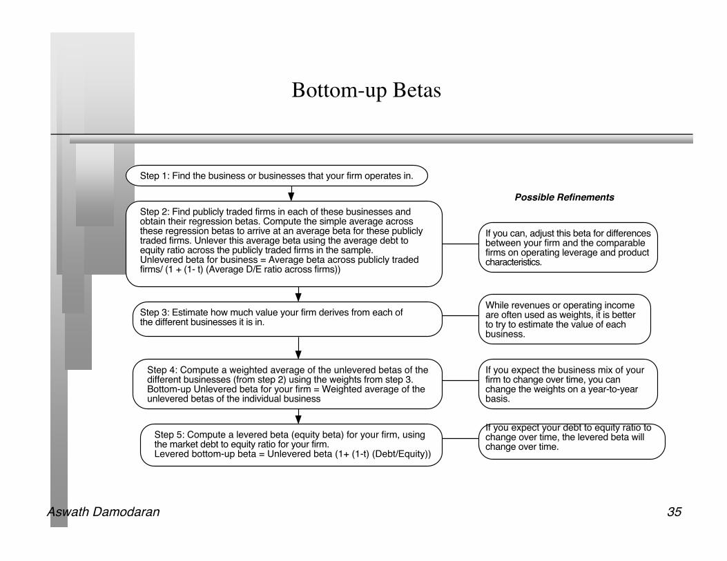
Bottom-up Betas
Step 1: Find the business or businesses that your firm operates in.
Step 2: Find publicly traded firms in each of these businesses and obtain their regression betas. Compute the simple average across these regression betas to arrive at an average beta for these publicly traded firms. Unlever this average beta using the average debt to equity ratio across the publicly traded firms in the sample.Unlevered beta for business = Average beta across publicly traded firms/ (1 + (1- t) (Average D/E ratio across firms))
If you can, adjust this beta for differencesbetween your firm and the comparablefirms on operating leverage and product characteristics.
Step 3: Estimate how much value your firm derives from each of the different businesses it is in.
While revenues or operating income are often used as weights, it is better to try to estimate the value of each business.
Step 4: Compute a weighted average of the unlevered betas of the different businesses (from step 2) using the weights from step 3.Bottom-up Unlevered beta for your firm = Weighted average of the unlevered betas of the individual business
Step 5: Compute a levered beta (equity beta) for your firm, using the market debt to equity ratio for your firm. Levered bottom-up beta = Unlevered beta (1+ (1-t) (Debt/Equity))
If you expect the business mix of your firm to change over time, you can change the weights on a year-to-year basis.
If you expect your debt to equity ratio to change over time, the levered beta will change over time.
Possible Refinements

Aswath Damodaran 36
BMW’s Bottom-up Beta
Business EBIT Value/EBIT Unlevered beta Value WeightAutomobiles 3052 7.15 1.02 21,822 88%Financing 569 5.25 0.81 2,987 12%Firm 0.99Levered Beta = Unlevered Beta ( 1 + (1- tax rate) (D/E Ratio)
= 0.99 ( 1 + (1-.4021) (.2531)) = 1.14

Aswath Damodaran 37
Amazon’s Bottom-up Beta
Unlevered beta for firms in internet retailing = 1.60Unlevered beta for firms in specialty retailing = 1.00
Amazon is a specialty retailer, but its risk currently seems to be determined by the factthat it is an online retailer. Hence we will use the beta of internet companies to beginthe valuation
By the fifth year, we are estimating substantial revenues for Amazon and we move thebeta towards to beta of the retailing business.
Aswath Damodaran 38
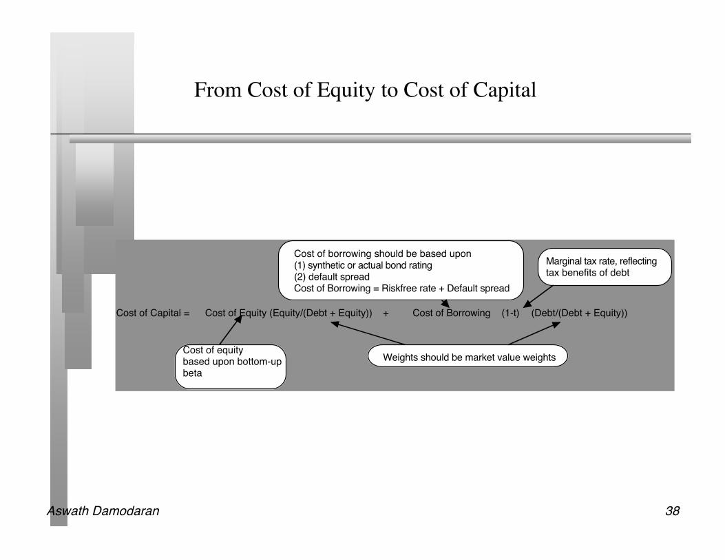
From Cost of Equity to Cost of Capital
Cost of Capital = Cost of Equity (Equity/(Debt + Equity)) + Cost of Borrowing (1-t) (Debt/(Debt + Equity))
Cost of borrowing should be based upon(1) synthetic or actual bond rating(2) default spreadCost of Borrowing = Riskfree rate + Default spread
Marginal tax rate, reflectingtax benefits of debt
Weights should be market value weightsCost of equitybased upon bottom-upbeta

Aswath Damodaran 39
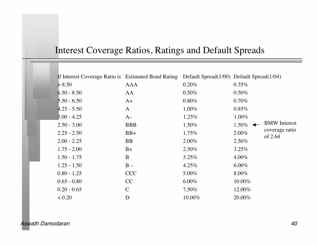
Bond Rating: Synthetic versus Actual
If a firm is rated, its bond rating represents the ratings agency’s judgment ofthe default risk of a firm. BMW is rated A+ by S&P.
The rating for a firm can be estimated using the financial characteristics of thefirm. In its simplest form, the rating can be estimated from the interestcoverage ratio
Interest Coverage Ratio = EBIT / Interest Expenses For BMW’s interest coverage ratio, we used the interest expenses and EBIT
from 2003.Interest Coverage Ratio = 3353/ 811 = 2.64
Amazon.com has negative operating income; this yields a negative interestcoverage ratio, which should suggest a low rating. We computed an averageinterest coverage ratio of 2.82 over the next 5 years.
Aswath Damodaran 40
Interest Coverage Ratios, Ratings and Default Spreads
If Interest Coverage Ratio is Estimated Bond Rating Default Spread(1/00) Default Spread(1/04)> 8.50 AAA 0.20% 0.35%6.50 - 8.50 AA 0.50% 0.50%5.50 - 6.50 A+ 0.80% 0.70%4.25 - 5.50 A 1.00% 0.85%3.00 - 4.25 A– 1.25% 1.00%2.50 - 3.00 BBB 1.50% 1.50%2.25 - 2.50 BB+ 1.75% 2.00%2.00 - 2.25 BB 2.00% 2.50%1.75 - 2.00 B+ 2.50% 3.25%1.50 - 1.75 B 3.25% 4.00%1.25 - 1.50 B – 4.25% 6.00%0.80 - 1.25 CCC 5.00% 8.00%0.65 - 0.80 CC 6.00% 10.00%0.20 - 0.65 C 7.50% 12.00%< 0.20 D 10.00% 20.00%
BMW Interestcoverage ratioof 2.64
Aswath Damodaran 41
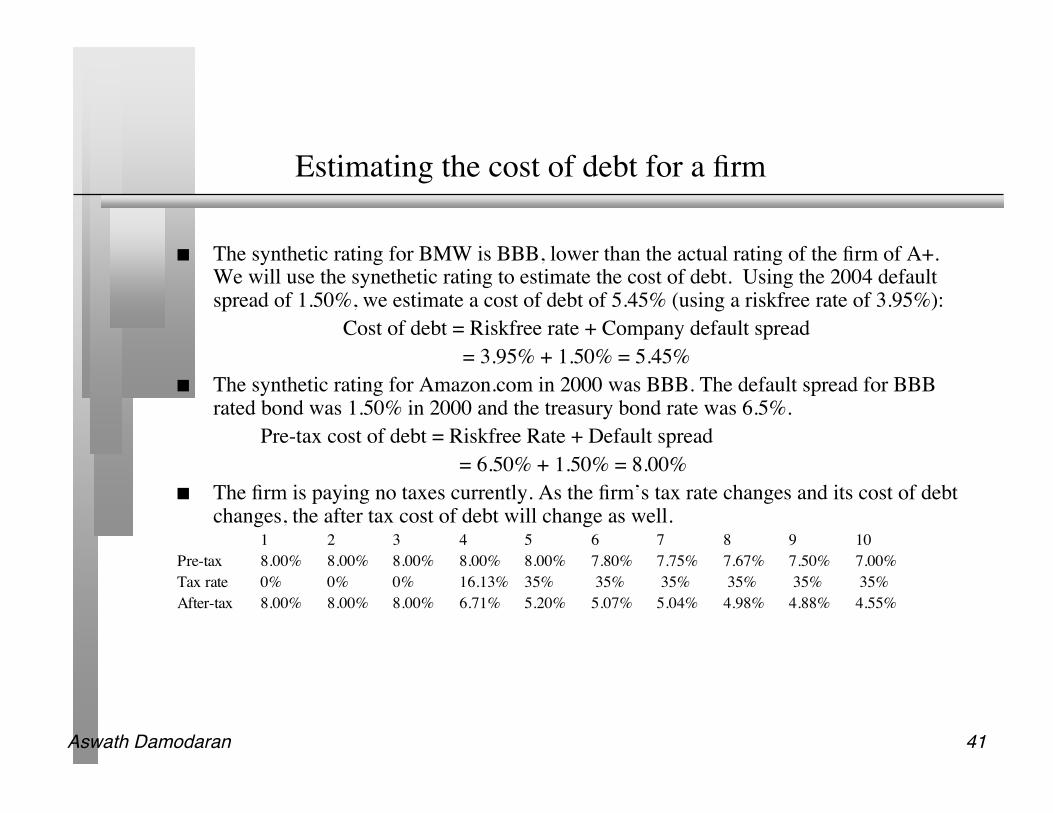
Estimating the cost of debt for a firm
The synthetic rating for BMW is BBB, lower than the actual rating of the firm of A+.We will use the synethetic rating to estimate the cost of debt. Using the 2004 defaultspread of 1.50%, we estimate a cost of debt of 5.45% (using a riskfree rate of 3.95%):
Cost of debt = Riskfree rate + Company default spread = 3.95% + 1.50% = 5.45%
The synthetic rating for Amazon.com in 2000 was BBB. The default spread for BBBrated bond was 1.50% in 2000 and the treasury bond rate was 6.5%.
Pre-tax cost of debt = Riskfree Rate + Default spread= 6.50% + 1.50% = 8.00%
The firm is paying no taxes currently. As the firm’s tax rate changes and its cost of debtchanges, the after tax cost of debt will change as well.
1 2 3 4 5 6 7 8 9 10Pre-tax 8.00% 8.00% 8.00% 8.00% 8.00% 7.80% 7.75% 7.67% 7.50% 7.00%Tax rate 0% 0% 0% 16.13% 35% 35% 35% 35% 35% 35%After-tax 8.00% 8.00% 8.00% 6.71% 5.20% 5.07% 5.04% 4.98% 4.88% 4.55%
Aswath Damodaran 42
Weights for the Cost of Capital Computation
The weights used to compute the cost of capital should be the market valueweights for debt and equity.
There is an element of circularity that is introduced into every valuation bydoing this, since the values that we attach to the firm and equity at the end ofthe analysis are different from the values we gave them at the beginning.
As a general rule, the debt that you should subtract from firm value to arriveat the value of equity should be the same debt that you used to compute thecost of capital.
Aswath Damodaran 43
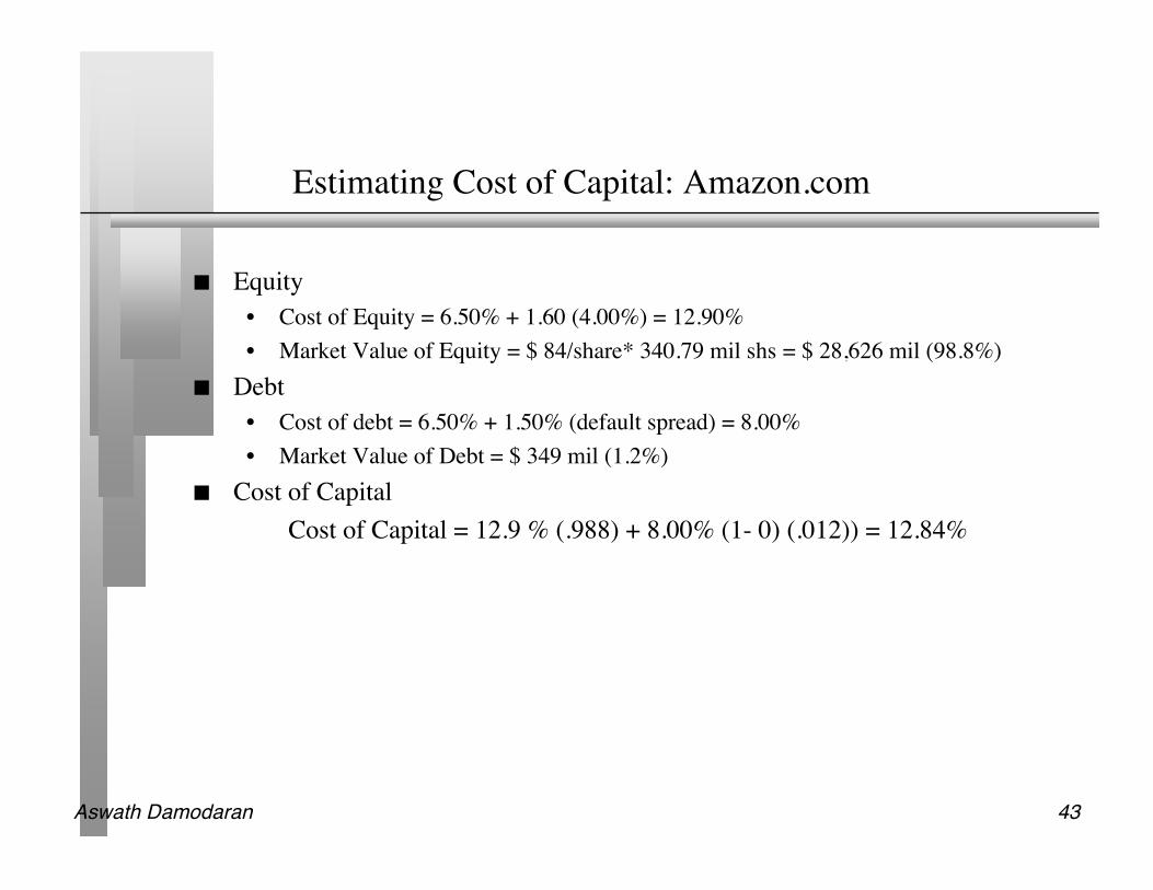
Estimating Cost of Capital: Amazon.com
Equity• Cost of Equity = 6.50% + 1.60 (4.00%) = 12.90%• Market Value of Equity = $ 84/share* 340.79 mil shs = $ 28,626 mil (98.8%)
Debt• Cost of debt = 6.50% + 1.50% (default spread) = 8.00%• Market Value of Debt = $ 349 mil (1.2%)
Cost of CapitalCost of Capital = 12.9 % (.988) + 8.00% (1- 0) (.012)) = 12.84%

Aswath Damodaran 44
Estimating Cost of Capital: BMW
Equity• Cost of Equity = 3.95% + 1.14 (3.83%) + 0.08 (2.50%) = 8.52%• Market Value of Equity =22,596 million Euros (80.15%)
Debt• Cost of debt = 3.95%+1.50%= 5.45%• Market Value of Debt = 5,597 million Euros (19.85%)
Cost of CapitalCost of Capital = 8.52 % (.8015) + 5.45% (1- .4021) (0.1985)) = 7.47%
The book value of equity at BMW is 16,150 million EurosThe book value of debt at BMW is 5,499 million; Interest expense is 336 mil; Average
maturity of debt = 3 yearsEstimated market value of debt = 336 million (PV of annuity, 3 years, 5.45%) + 5,499
million/1.05453 = 5,597 million Euros

Aswath Damodaran 45
II. Estimating Cash Flows to Firm
Earnings before interest and taxes
- Tax rate * EBIT
= EBIT ( 1- tax rate)
- (Capital Expenditures - Depreciation)
- Change in non-cash working capital
= Free Cash flow to the firm (FCFF)
Update- Trailing Earnings- Unofficial numbers
Normalize- History- Industry
Cleanse operating items of- Financial Expenses- Capital Expenses- Non-recurring expenses
Operating leases- Convert into debt- Adjust operating income
R&D Expenses- Convert into asset- Adjust operating income
Tax rate- can be effective for near future, but move to marginal- reflect net operating losses
Include- R&D- Acquisitions
Defined asNon-cash CA- Non-debt CL

Aswath Damodaran 46
The Importance of Updating
The operating income and revenue that we use in valuation should be updatednumbers. One of the problems with using financial statements is that they aredated.
As a general rule, it is better to use 12-month trailing estimates for earningsand revenues than numbers for the most recent financial year. This rulebecomes even more critical when valuing companies that are evolving andgrowing rapidly.
Last 10-K Trailing 12-monthRevenues $ 610 million $1,117 millionEBIT - $125 million - $ 410 million
Aswath Damodaran 47
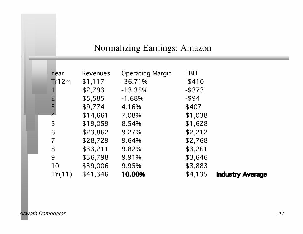
Normalizing Earnings: Amazon
Year Revenues Operating Margin EBITTr12m $1,117 -36.71% -$4101 $2,793 -13.35% -$3732 $5,585 -1.68% -$943 $9,774 4.16% $4074 $14,661 7.08% $1,0385 $19,059 8.54% $1,6286 $23,862 9.27% $2,2127 $28,729 9.64% $2,7688 $33,211 9.82% $3,2619 $36,798 9.91% $3,64610 $39,006 9.95% $3,883TY(11) $41,346 10.00% $4,135 Industry Average

Aswath Damodaran 48
Operating Leases at The Home Depot in 1998
The pre-tax cost of debt at the Home Depot is 6.25%Yr Operating Lease Expense Present Value 1 $ 294 $ 277 2 $ 291 $ 258 3 $ 264 $ 220 4 $ 245 $ 192 5 $ 236 $ 174 6-15 $ 270 $ 1,450 (PV of 10-yr annuity)
Present Value of Operating Leases =$ 2,571 Debt outstanding at the Home Depot = $1,205 + $2,571 = $3,776 mil
(The Home Depot has other debt outstanding of $1,205 million) Adjusted Operating Income = $2,016 + 2,571 (.0625) = $2,177 mil
Aswath Damodaran 49
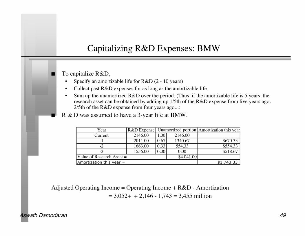
Capitalizing R&D Expenses: BMW
To capitalize R&D,• Specify an amortizable life for R&D (2 - 10 years)• Collect past R&D expenses for as long as the amortizable life• Sum up the unamortized R&D over the period. (Thus, if the amortizable life is 5 years, the
research asset can be obtained by adding up 1/5th of the R&D expense from five years ago,2/5th of the R&D expense from four years ago...:
R & D was assumed to have a 3-year life at BMW.
Adjusted Operating Income = Operating Income + R&D - Amortization= 3,052+ + 2,146 - 1,743 = 3,455 million
Year R&D Expense Amortization this yearCurrent 2146.00 1.00 2146.00
-1 2011.00 0.67 1340.67 $670.33-2 1663.00 0.33 554.33 $554.33-3 1556.00 0.00 0.00 $518.67
$4,041.00$1,743.33
Value of Research Asset =Amortization this year =
Unamortized portion
Aswath Damodaran 50
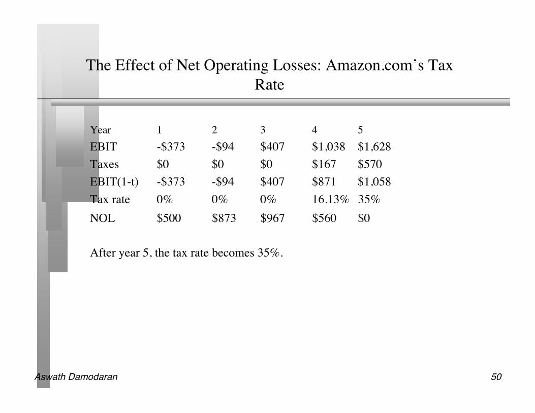
The Effect of Net Operating Losses: Amazon.com’s TaxRate
Year 1 2 3 4 5EBIT -$373 -$94 $407 $1,038 $1,628Taxes $0 $0 $0 $167 $570EBIT(1-t) -$373 -$94 $407 $871 $1,058Tax rate 0% 0% 0% 16.13% 35%NOL $500 $873 $967 $560 $0
After year 5, the tax rate becomes 35%.

Aswath Damodaran 51
Estimating Actual FCFF: BMW
EBIT = 3,455 million Euros Tax rate = 41.21% Net Capital expenditures = Cap Ex - Depreciation = 9,339 -8,652 = 687
million Change in Working Capital = + 583 million (Increase)Estimating FCFFCurrent EBIT * (1 - tax rate) = 3,455 (1-.4021) = 2,277 Million - (Capital Spending - Depreciation) 687 - Change in Working Capital 583Current FCFF 958 Million Euros

Aswath Damodaran 52
Estimating FCFF: Amazon.com
EBIT (Trailing 1999) = -$ 410 million Tax rate used = 0% (Assumed Effective = Marginal) Capital spending (Trailing 1999) = $ 243 million Depreciation (Trailing 1999) = $ 31 million Non-cash Working capital Change (1999) = - 80 million Estimating FCFF (1999)
Current EBIT * (1 - tax rate) = - 410 (1-0) = - $410 million - (Capital Spending - Depreciation) = $212 million - Change in Working Capital = -$ 80 millionCurrent FCFF = - $542 million

Aswath Damodaran 53
IV. Expected Growth in EBIT and Fundamentals
Reinvestment Rate and Return on CapitalgEBIT = (Net Capital Expenditures + Change in WC)/EBIT(1-t) * ROC
= Reinvestment Rate * ROC Proposition: No firm can expect its operating income to grow over time
without reinvesting some of the operating income in net capital expendituresand/or working capital.
Proposition: The net capital expenditure needs of a firm, for a given growthrate, should be inversely proportional to the quality of its investments.

Aswath Damodaran 54
Return on Capital Computation: BMW
After-tax Operating Income2,227 million Euros
Book Value of Equity13,871+4041 = 17,509 million Euros
Stated Book value of Equity13,871 million
Research Asset4,041 million
Book Value of Debt6,769 million Euros
Book value of debt and equity from end of prior year
/ Book Value of Capital from end of prior year17,509 + 6,769 = 24,278 million Euros
Return on Capital in 2003 = 9.17%
Aswath Damodaran 55
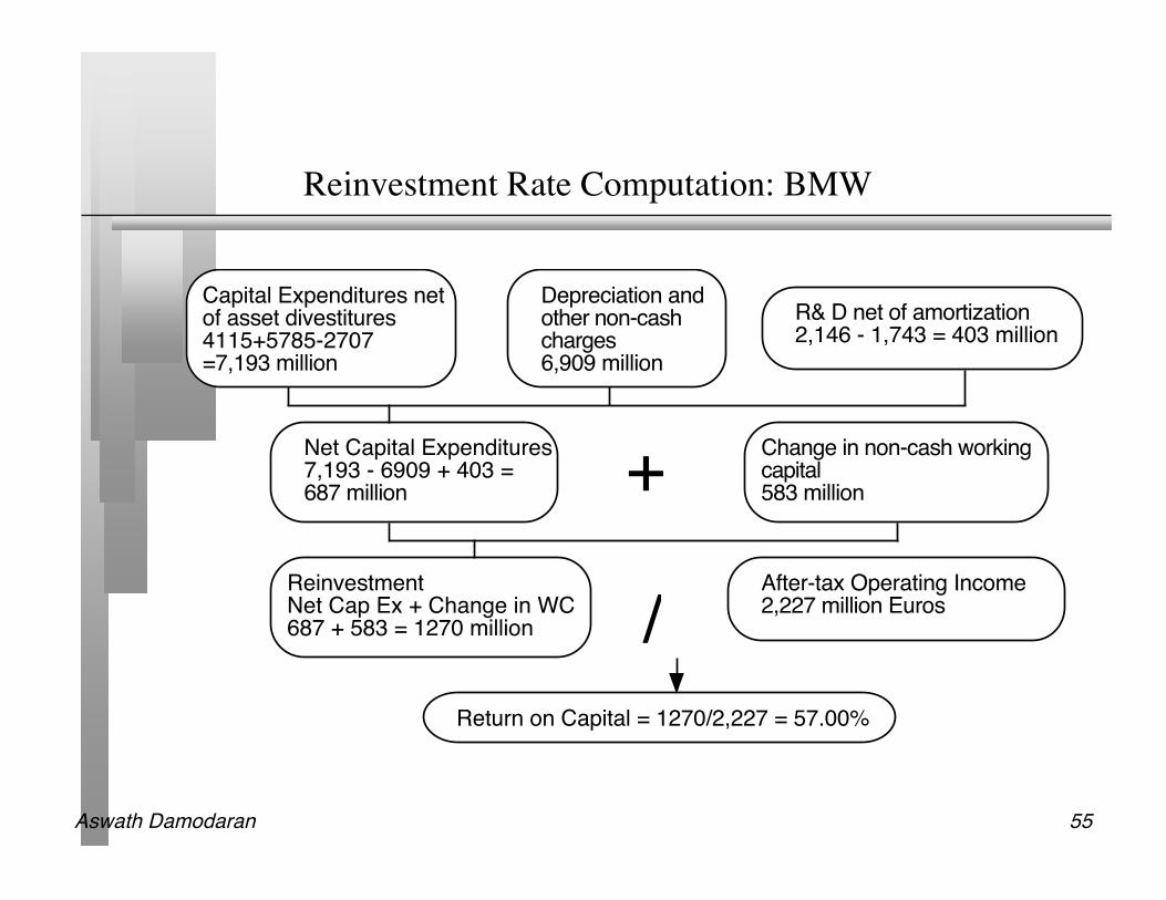
Reinvestment Rate Computation: BMW
Capital Expenditures net of asset divestitures4115+5785-2707 =7,193 million
Depreciation and other non-cash charges 6,909 million
Net Capital Expenditures7,193 - 6909 + 403 = 687 million
R& D net of amortization2,146 - 1,743 = 403 million
+Change in non-cash working capital583 million
Reinvestment Net Cap Ex + Change in WC687 + 583 = 1270 million /
After-tax Operating Income2,227 million Euros
Return on Capital = 1270/2,227 = 57.00%
Aswath Damodaran 56
Revenue Growth and Operating Margins
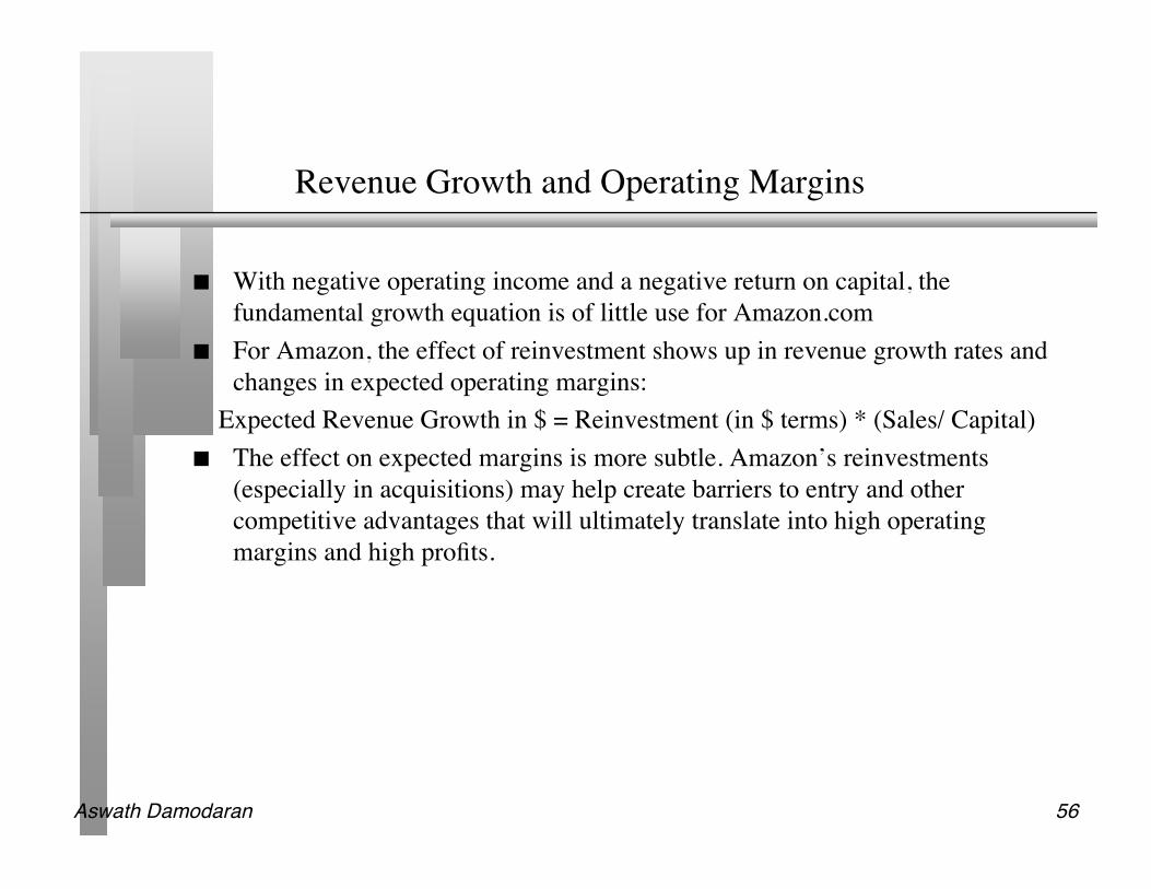
With negative operating income and a negative return on capital, thefundamental growth equation is of little use for Amazon.com
For Amazon, the effect of reinvestment shows up in revenue growth rates andchanges in expected operating margins:
Expected Revenue Growth in $ = Reinvestment (in $ terms) * (Sales/ Capital) The effect on expected margins is more subtle. Amazon’s reinvestments
(especially in acquisitions) may help create barriers to entry and othercompetitive advantages that will ultimately translate into high operatingmargins and high profits.

Aswath Damodaran 57
Growth in Revenues, Earnings and Reinvestment: Amazon
Year Revenue Chg in Reinvestment Chg Rev/ Chg Reinvestment ROCGrowth Revenue
1 150.00% $1,676 $559 3.00 -76.62%2 100.00% $2,793 $931 3.00 -8.96%3 75.00% $4,189 $1,396 3.00 20.59%4 50.00% $4,887 $1,629 3.00 25.82%5 30.00% $4,398 $1,466 3.00 21.16%6 25.20% $4,803 $1,601 3.00 22.23%7 20.40% $4,868 $1,623 3.00 22.30%8 15.60% $4,482 $1,494 3.00 21.87%9 10.80% $3,587 $1,196 3.00 21.19%10 6.00% $2,208 $736 3.00 20.39%Assume that firm can earn high returns because of established economies of scale.

Aswath Damodaran 58
V. Growth Patterns
A key assumption in all discounted cash flow models is the period of highgrowth, and the pattern of growth during that period. In general, we can makeone of three assumptions:
• there is no high growth, in which case the firm is already in stable growth• there will be high growth for a period, at the end of which the growth rate will
drop to the stable growth rate (2-stage)• there will be high growth for a period, at the end of which the growth rate will
decline gradually to a stable growth rate(3-stage)
Stable Growth 2-Stage Growth 3-Stage Growth

Aswath Damodaran 59
Determinants of Growth Patterns
Size of the firm• Success usually makes a firm larger. As firms become larger, it becomes much
more difficult for them to maintain high growth rates Current growth rate
• While past growth is not always a reliable indicator of future growth, there is acorrelation between current growth and future growth. Thus, a firm growing at30% currently probably has higher growth and a longer expected growth periodthan one growing 10% a year now.
Barriers to entry and differential advantages• Ultimately, high growth comes from high project returns, which, in turn, comes
from barriers to entry and differential advantages.• The question of how long growth will last and how high it will be can therefore be
framed as a question about what the barriers to entry are, how long they will stayup and how strong they will remain.
Aswath Damodaran 60
Stable Growth Characteristics
In stable growth, firms should have the characteristics of other stable growthfirms. In particular,
• The risk of the firm, as measured by beta and ratings, should reflect that of a stablegrowth firm.
– Beta should move towards one– The cost of debt should reflect the safety of stable firms (BBB or higher)
• The debt ratio of the firm might increase to reflect the larger and more stableearnings of these firms.
– The debt ratio of the firm might moved to the optimal or an industry average– If the managers of the firm are deeply averse to debt, this may never happen
• The reinvestment rate of the firm should reflect the expected growth rate and thefirm’s return on capital
– Reinvestment Rate = Expected Growth Rate / Return on Capital
Aswath Damodaran 61
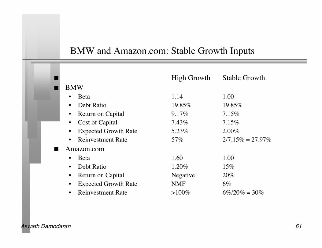
BMW and Amazon.com: Stable Growth Inputs
High Growth Stable Growth BMW
• Beta 1.14 1.00• Debt Ratio 19.85% 19.85%• Return on Capital 9.17% 7.15%• Cost of Capital 7.43% 7.15%• Expected Growth Rate 5.23% 2.00%• Reinvestment Rate 57% 2/7.15% = 27.97%
Amazon.com• Beta 1.60 1.00• Debt Ratio 1.20% 15%• Return on Capital Negative 20%• Expected Growth Rate NMF 6%• Reinvestment Rate >100% 6%/20% = 30%

Aswath Damodaran 62
Dealing with Cash and Marketable Securities
The simplest and most direct way of dealing with cash and marketablesecurities is to keep them out of the valuation - the cash flows should bebefore interest income from cash and securities, and the discount rate shouldnot be contaminated by the inclusion of cash. (Use betas of the operatingassets alone to estimate the cost of equity).
Once the firm has been valued, add back the value of cash and marketablesecurities.
• If you have a particularly incompetent management, with a history of overpayingon acquisitions, markets may discount the value of this cash.
Aswath Damodaran 63
Dealing with Cross Holdings
When the holding is a majority, active stake, the value that we obtain from thecash flows includes the share held by outsiders. While their holding ismeasured in the balance sheet as a minority interest, it is at book value. To getthe correct value, we need to subtract out the estimated market value of theminority interests from the firm value.
When the holding is a minority, passive interest, the problem is a differentone. The firm shows on its income statement only the share of dividends itreceives on the holding. Using only this income will understate the value ofthe holdings. In fact, we have to value the subsidiary as a separate entity toget a measure of the market value of this holding.
Proposition 1: It is almost impossible to correctly value firms with minority,passive interests in a large number of private subsidiaries.

Aswath Damodaran 64
Non-debt Obligations
Pension fund obligations: If pension fund assets are not intermingled withother assets, only the underfunded portion of pension fund liabilities shouldbe considered. If pension fund assets are intermingled, all of the pension fundobligations should be considered.
Lawsuit obligations: If lawsuits are pending against the firm, the expectedvalue (based on the likelihood of losing the lawsuits and the penalty if thatoccurs) of the lawsuits should be deducted.
Other obligations: Deferred tax liabilities, employee health care benefits andsocial cost obligations can also be deducted, though the rationale has to beclearly specified.

Aswath Damodaran 65
BMW: Towards the final value
Present Value of FCFF in high growth phase = $4,497.35Present Value of Terminal Value of Firm = $30,133.44Value of operating assets of the firm = $34,630.79Value of Cash, Marketable Securities & Non-operating assets = $4,123.00Value of Firm = $38,753.79Market Value of outstanding debt = $5,597.04Non-debt obligations and liabilities = $7,517.00Market Value of Equity = $25,639.75
Market Value of Equity/share = $38.07
Aswath Damodaran 66
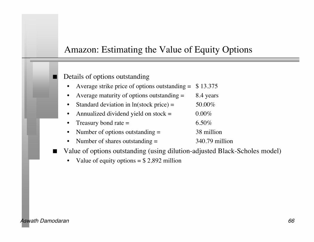
Amazon: Estimating the Value of Equity Options
Details of options outstanding• Average strike price of options outstanding = $ 13.375• Average maturity of options outstanding = 8.4 years• Standard deviation in ln(stock price) = 50.00%• Annualized dividend yield on stock = 0.00%• Treasury bond rate = 6.50%• Number of options outstanding = 38 million• Number of shares outstanding = 340.79 million
Value of options outstanding (using dilution-adjusted Black-Scholes model)• Value of equity options = $ 2,892 million
Aswath Damodaran 67
Forever
Terminal Value= 1881/(.0961-.06)=52,148
Cost of Equity12.90%
Cost of Debt6.5%+1.5%=8.0%Tax rate = 0% -> 35%
WeightsDebt= 1.2% -> 15%
Value of Op Assets $ 14,910+ Cash $ 26= Value of Firm $14,936- Value of Debt $ 349= Value of Equity $14,587- Equity Options $ 2,892Value per share $ 34.32
Riskfree Rate :T. Bond rate = 6.5%
+Beta1.60 -> 1.00 X
Risk Premium4%
Internet/Retail
Operating Leverage
Current D/E: 1.21%
Base EquityPremium
Country RiskPremium
CurrentRevenue$ 1,117
CurrentMargin:-36.71%
Reinvestment:Cap ex includes acquisitionsWorking capital is 3% of revenues
Sales TurnoverRatio: 3.00
CompetitiveAdvantages
Revenue Growth:42%
Expected Margin: -> 10.00%
Stable Growth
StableRevenueGrowth: 6%
StableOperatingMargin: 10.00%
Stable ROC=20%Reinvest 30% of EBIT(1-t)
EBIT-410m
NOL:500 m
$41,346
10.00%
35.00%
$2,688
$ 807
$1,881
Term. Year
2 431 5 6 8 9 107
Cost of Equity 12.90% 12.90% 12.90% 12.90% 12.90% 12.42% 12.30% 12.10% 11.70% 10.50%
Cost of Debt 8.00% 8.00% 8.00% 8.00% 8.00% 7.80% 7.75% 7.67% 7.50% 7.00%
AT cost of debt 8.00% 8.00% 8.00% 6.71% 5.20% 5.07% 5.04% 4.98% 4.88% 4.55%
Cost of Capital 12.84% 12.84% 12.84% 12.83% 12.81% 12.13% 11.96% 11.69% 11.15% 9.61%
Revenues $2,793 5,585 9,774 14,661 19,059 23,862 28,729 33,211 36,798 39,006
EBIT -$373 -$94 $407 $1,038 $1,628 $2,212 $2,768 $3,261 $3,646 $3,883
EBIT (1-t) -$373 -$94 $407 $871 $1,058 $1,438 $1,799 $2,119 $2,370 $2,524
- Reinvestment $559 $931 $1,396 $1,629 $1,466 $1,601 $1,623 $1,494 $1,196 $736
FCFF -$931 -$1,024 -$989 -$758 -$408 -$163 $177 $625 $1,174 $1,788
Amazon.comJanuary 2000Stock Price = $ 84

Aswath Damodaran 68
Amazon.com: Break Even at $84?
6% 8% 10% 12% 14%
30% (1.94)$ 2.95$ 7.84$ 12.71$ 17.57$
35% 1.41$ 8.37$ 15.33$ 22.27$ 29.21$
40% 6.10$ 15.93$ 25.74$ 35.54$ 45.34$
45% 12.59$ 26.34$ 40.05$ 53.77$ 67.48$
50% 21.47$ 40.50$ 59.52$ 78.53$ 97.54$
55% 33.47$ 59.60$ 85.72$ 111.84$ 137.95$
60% 49.53$ 85.10$ 120.66$ 156.22$ 191.77$

Aswath Damodaran 69
Forever
Terminal Value= 1064/(.0876-.05)=$ 28,310
Cost of Equity13.81%
Cost of Debt5.1%+4.75%= 9.85%Tax rate = 0% -> 35%
WeightsDebt= 27.38% -> 15%
Value of Op Assets $ 7,967+ Cash & Non-op $ 1,263= Value of Firm $ 9,230- Value of Debt $ 1,890= Value of Equity $ 7,340- Equity Options $ 748Value per share $ 18.74
Riskfree Rate :T. Bond rate = 5.1%
+Beta2.18-> 1.10 X
Risk Premium4%
Internet/Retail
Operating Leverage
Current D/E: 37.5%
Base EquityPremium
Country RiskPremium
CurrentRevenue$ 2,465
CurrentMargin:-34.60%
Reinvestment:Cap ex includes acquisitionsWorking capital is 3% of revenues
Sales TurnoverRatio: 3.02
CompetitiveAdvantages
Revenue Growth:25.41%
Expected Margin: -> 9.32%
Stable Growth
StableRevenueGrowth: 5%
StableOperatingMargin: 9.32%
Stable ROC=16.94%Reinvest 29.5% of EBIT(1-t)
EBIT-853m
NOL:1,289 m
$24,912
$2,322
$1,509
$ 445
$1,064
Term. Year
2 431 5 6 8 9 107
Debt Ratio 27.27% 27.27% 27.27% 27.27% 27.27% 24.81% 24.20% 23.18% 21.13% 15.00%
Beta 2.18 2.18 2.18 2.18 2.18 1.96 1.75 1.53 1.32 1.10
Cost of Equity 13.81% 13.81% 13.81% 13.81% 13.81% 12.95% 12.09% 11.22% 10.36% 9.50%
AT cost of debt 10.00% 10.00% 10.00% 10.00% 9.06% 6.11% 6.01% 5.85% 5.53% 4.55%
Cost of Capital 12.77% 12.77% 12.77% 12.77% 12.52% 11.25% 10.62% 9.98% 9.34% 8.76%
Amazon.comJanuary 2001Stock price = $14
Revenues $4,314 $6,471 $9,059 $11,777 $14,132 $16,534 $18,849 $20,922 $22,596 $23,726 $24,912EBIT -$703 -$364 $54 $499 $898 $1,255 $1,566 $1,827 $2,028 $2,164 $2,322EBIT(1-t) -$703 -$364 $54 $499 $898 $1,133 $1,018 $1,187 $1,318 $1,406 $1,509 - Reinvestment $612 $714 $857 $900 $780 $796 $766 $687 $554 $374 $445FCFF -$1,315 -$1,078 -$803 -$401 $118 $337 $252 $501 $764 $1,032 $1,064

Aswath Damodaran 70
Current Cashflow to FirmEBIT(1-t) : 2,227- Nt CpX 687 - Chg WC 583= FCFF ! 958Reinvestment Rate=(687+583)/2227
= 57%
Expected Growth in EBIT (1-t).57*.0917=.05235.23%
Stable Growthg = 2%; Beta = 1.00;Country Premium= 1.5%Cost of capital = 7.15% ROC= 7.15%; Tax rate=37%Reinvestment Rate=g/ROC
=2/ 7.15= 27.97%
Terminal Value5= 2225/(.0715-.02) = 43,205
Cost of Equity 8.52%
Cost of Debt(3.95%+1.50%)(1-.4021)= 3.26%
WeightsE = 80.15% D = 19.85%
Discount at $ Cost of Capital (WACC) = 8.52% (.8015) + 3.26% (0.1985) = 7.47%
Op. Assets! 34,631+ Cash: 4,123- Debt 5,597- Non-Debt 7,517=Equity 25,640
Value/Sh ! 38.07
Riskfree Rate:Euro Riskfree Rate= 3.95%
+Beta 1.14 X
Mature market premium 3.83 %
Unlevered Beta for Sectors: 0.99
Firm’s D/ERatio: 24.77%
BMW: Status Quo (Euros) Reinvestment Rate 57%
Return on Capital9.17%
Term Yr 3089 - 864= 2225
+ Lambda0.08
XEmerg Market Equity Risk Premium2.50%
On Sept 23, 2004BMW Common = 33.50 Eu
Euro Cashflows
Year 1 2 3 4 5EBIT (1-t) ! 2,344 ! 2,467 ! 2,596 ! 2,731 ! 2,874Reinvestment ! 1,336 ! 1,406 ! 1,479 ! 1,557 ! 1,638FCFF ! 1,008 ! 1,061 ! 1,116 ! 1,174 ! 1,236
g=2%Tax rate changes
Aswath Damodaran 71
Value Enhancement: Back to Basics
Aswath Damodaranhttp://www.damodaran.com

Aswath Damodaran 72
Price Enhancement versus Value Enhancement

Aswath Damodaran 73
The Paths to Value Creation
Using the DCF framework, there are four basic ways in which the value of afirm can be enhanced:
• The cash flows from existing assets to the firm can be increased, by either– increasing after-tax earnings from assets in place or– reducing reinvestment needs (net capital expenditures or working capital)
• The expected growth rate in these cash flows can be increased by either– Increasing the rate of reinvestment in the firm– Improving the return on capital on those reinvestments
• The length of the high growth period can be extended to allow for more years ofhigh growth.
• The cost of capital can be reduced by– Reducing the operating risk in investments/assets– Changing the financial mix– Changing the financing composition
Aswath Damodaran 74
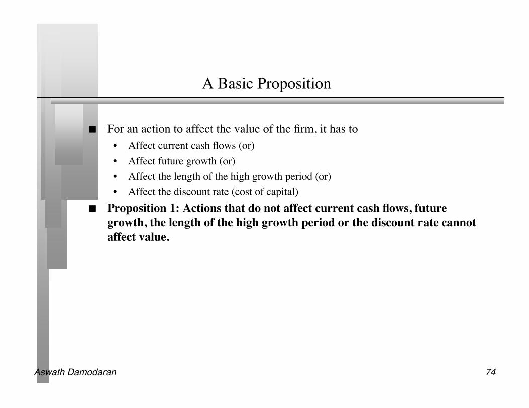
A Basic Proposition
For an action to affect the value of the firm, it has to• Affect current cash flows (or)• Affect future growth (or)• Affect the length of the high growth period (or)• Affect the discount rate (cost of capital)
Proposition 1: Actions that do not affect current cash flows, futuregrowth, the length of the high growth period or the discount rate cannotaffect value.

Aswath Damodaran 75
Value-Neutral Actions
Stock splits and stock dividends change the number of units of equity in a firm, butcannot affect firm value since they do not affect cash flows, growth or risk.
Accounting decisions that affect reported earnings but not cash flows should have noeffect on value.
• Changing inventory valuation methods from FIFO to LIFO or vice versa in financial reportsbut not for tax purposes
• Changing the depreciation method used in financial reports (but not the tax books) fromaccelerated to straight line depreciation
• Major non-cash restructuring charges that reduce reported earnings but are not tax deductible• Using pooling instead of purchase in acquisitions cannot change the value of a target firm.
Decisions that create new securities on the existing assets of the firm (without alteringthe financial mix) such as tracking stock cannot create value, though they might affectperceptions and hence the price.

Aswath Damodaran 76
I. Ways of Increasing Cash Flows from Assets in Place
Revenues
* Operating Margin
= EBIT
- Tax Rate * EBIT
= EBIT (1-t)
+ Depreciation- Capital Expenditures- Chg in Working Capital= FCFF
Divest assets thathave negative EBIT
More efficient operations and cost cuttting: Higher Margins
Reduce tax rate- moving income to lower tax locales- transfer pricing- risk management
Live off past over- investment
Better inventory management and tighter credit policies
Aswath Damodaran 77
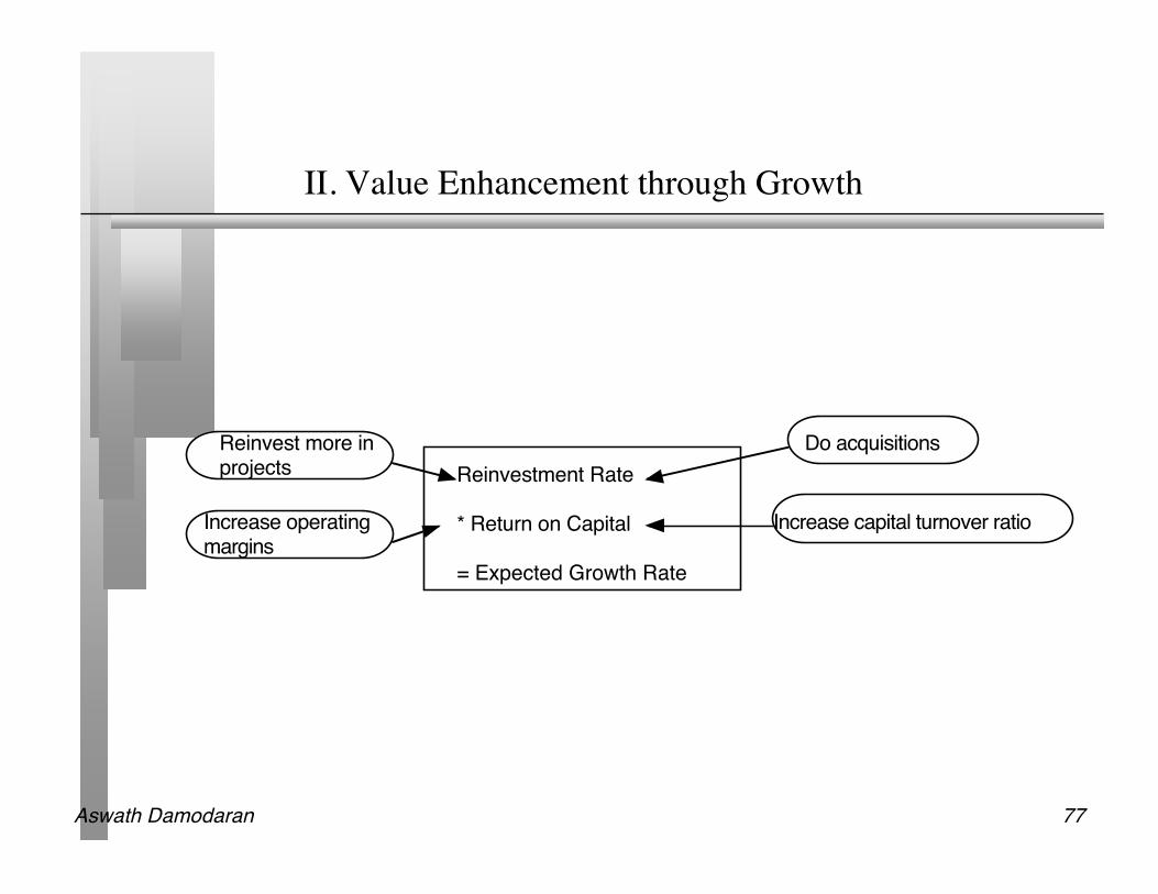
II. Value Enhancement through Growth
Reinvestment Rate
* Return on Capital
= Expected Growth Rate
Reinvest more inprojects
Do acquisitions
Increase operatingmargins
Increase capital turnover ratio

Aswath Damodaran 78
III. Building Competitive Advantages: Increase length of thegrowth period
Increase length of growth period
Build on existing competitive advantages
Find new competitive advantages
Brand name
Legal Protection
Switching Costs
Cost advantages

Aswath Damodaran 79
3.1: The Brand Name Advantage
Some firms are able to sustain above-normal returns and growth because theyhave well-recognized brand names that allow them to charge higher pricesthan their competitors and/or sell more than their competitors.
Firms that are able to improve their brand name value over time can increaseboth their growth rate and the period over which they can expect to grow atrates above the stable growth rate, thus increasing value.

Aswath Damodaran 80
Illustration: Valuing a brand name: Coca Cola
Coca Cola Generic Cola CompanyAT Operating Margin 18.56% 7.50%Sales/BV of Capital 1.67 1.67ROC 31.02% 12.53%Reinvestment Rate 65.00% (19.35%) 65.00% (47.90%)Expected Growth 20.16% 8.15%Length 10 years 10 yeaCost of Equity 12.33% 12.33%E/(D+E) 97.65% 97.65%AT Cost of Debt 4.16% 4.16%D/(D+E) 2.35% 2.35%Cost of Capital 12.13% 12.13%Value $115 $13

Aswath Damodaran 81
3.2: Patents and Legal Protection
The most complete protection that a firm can have from competitive pressureis to own a patent, copyright or some other kind of legal protection allowing itto be the sole producer for an extended period.
Note that patents only provide partial protection, since they cannot protect afirm against a competitive product that meets the same need but is not coveredby the patent protection.
Licenses and government-sanctioned monopolies also provide protectionagainst competition. They may, however, come with restrictions on excessreturns; utilities in the United States, for instance, are monopolies but areregulated when it comes to price increases and returns.
Aswath Damodaran 82
3.3: Switching Costs
Another potential barrier to entry is the cost associated with switching fromone firm’s products to another.
The greater the switching costs, the more difficult it is for competitors tocome in and compete away excess returns.
Firms that devise ways to increase the cost of switching from their products tocompetitors’ products, while reducing the costs of switching from competitorproducts to their own will be able to increase their expected length of growth.

Aswath Damodaran 83
3.4: Cost Advantages
There are a number of ways in which firms can establish a cost advantageover their competitors, and use this cost advantage as a barrier to entry:
• In businesses, where scale can be used to reduce costs, economies of scale can givebigger firms advantages over smaller firms
• Owning or having exclusive rights to a distribution system can provide firms witha cost advantage over its competitors.
• Owning or having the rights to extract a natural resource which is in restrictedsupply (The undeveloped reserves of an oil or mining company, for instance)
These cost advantages will show up in valuation in one of two ways:• The firm may charge the same price as its competitors, but have a much higher
operating margin.• The firm may charge lower prices than its competitors and have a much higher
capital turnover ratio.

Aswath Damodaran 84
Gauging Barriers to Entry
Which of the following barriers to entry are most likely to work for BMW? Brand Name Patents and Legal Protection Switching Costs Cost Advantages What about for Amazon.com? Brand Name Patents and Legal Protection Switching Costs Cost Advantages

Aswath Damodaran 85
Reducing Cost of Capital
Cost of Equity (E/(D+E) + Pre-tax Cost of Debt (D./(D+E)) = Cost of Capital
Change financing mix
Make product or service less discretionary to customers
Reduce operating leverage
Match debt to assets, reducing default risk
Changing product characteristics
More effective advertising
Outsourcing Flexible wage contracts &cost structure
Swaps Derivatives Hybrids
Aswath Damodaran 86
Amazon.com: Optimal Debt Ratio
Debt Ratio Beta Cost of Equity Bond Rating Interest rate on debt Tax Rate Cost of Debt (after-tax) WACC Firm Value (G)
0% 1.58 12.82% AAA 6.80% 0.00% 6.80% 12.82% $29,192
10% 1.76 13.53% D 18.50% 0.00% 18.50% 14.02% $24,566
20% 1.98 14.40% D 18.50% 0.00% 18.50% 15.22% $21,143
30% 2.26 15.53% D 18.50% 0.00% 18.50% 16.42% $18,509
40% 2.63 17.04% D 18.50% 0.00% 18.50% 17.62% $16,419
50% 3.16 19.15% D 18.50% 0.00% 18.50% 18.82% $14,719
60% 3.95 22.31% D 18.50% 0.00% 18.50% 20.02% $13,311
70% 5.27 27.58% D 18.50% 0.00% 18.50% 21.22% $12,125
80% 7.90 38.11% D 18.50% 0.00% 18.50% 22.42% $11,112
90% 15.81 69.73% D 18.50% 0.00% 18.50% 23.62% $10,237
Aswath Damodaran 87
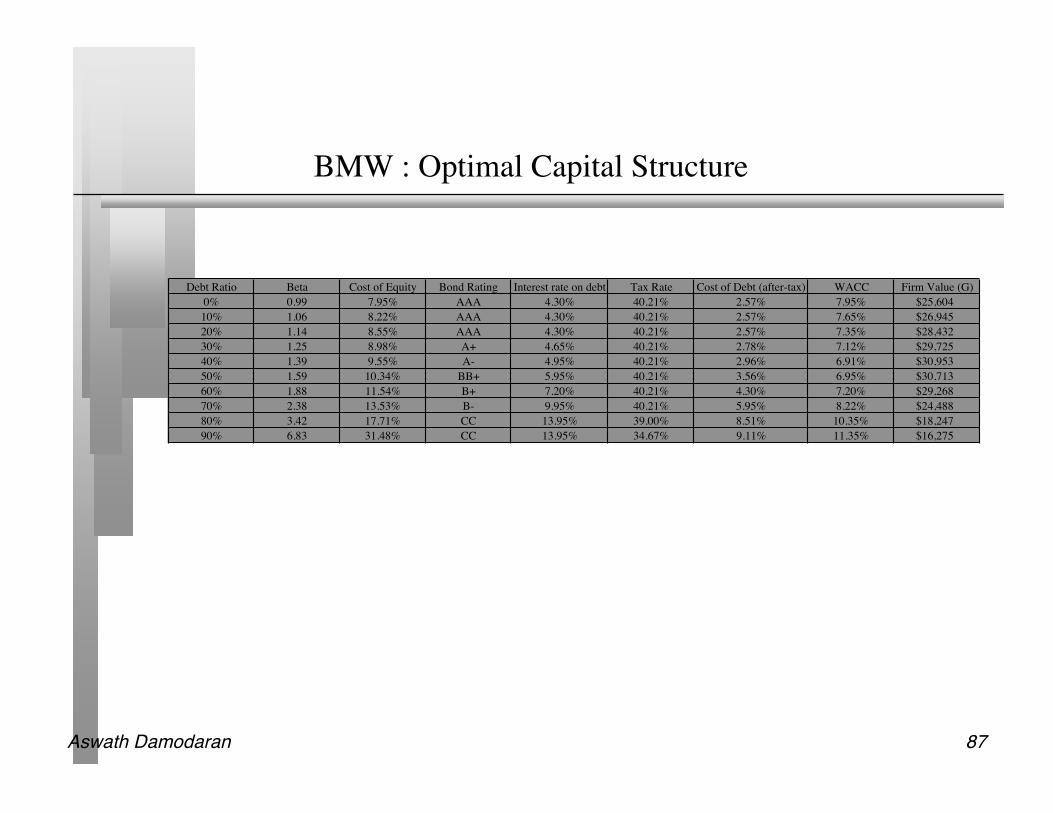
BMW : Optimal Capital Structure
Debt Ratio Beta Cost of Equity Bond Rating Interest rate on debt Tax Rate Cost of Debt (after-tax) WACC Firm Value (G)
0% 0.99 7.95% AAA 4.30% 40.21% 2.57% 7.95% $25,604
10% 1.06 8.22% AAA 4.30% 40.21% 2.57% 7.65% $26,945
20% 1.14 8.55% AAA 4.30% 40.21% 2.57% 7.35% $28,432
30% 1.25 8.98% A+ 4.65% 40.21% 2.78% 7.12% $29,725
40% 1.39 9.55% A- 4.95% 40.21% 2.96% 6.91% $30,953
50% 1.59 10.34% BB+ 5.95% 40.21% 3.56% 6.95% $30,713
60% 1.88 11.54% B+ 7.20% 40.21% 4.30% 7.20% $29,268
70% 2.38 13.53% B- 9.95% 40.21% 5.95% 8.22% $24,488
80% 3.42 17.71% CC 13.95% 39.00% 8.51% 10.35% $18,247
90% 6.83 31.48% CC 13.95% 34.67% 9.11% 11.35% $16,275
Aswath Damodaran 88
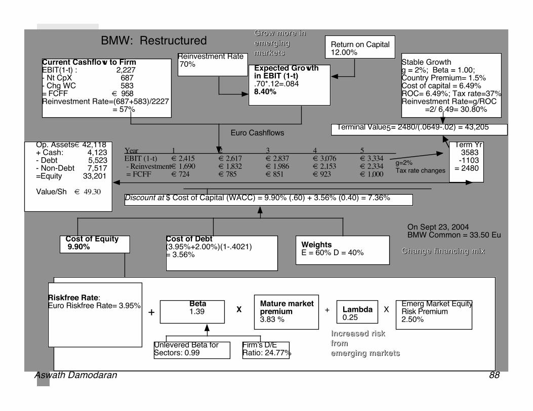
Current Cashflow to FirmEBIT(1-t) : 2,227- Nt CpX 687 - Chg WC 583= FCFF ! 958Reinvestment Rate=(687+583)/2227
= 57%
Expected Growth in EBIT (1-t).70*.12=.0848.40%
Stable Growthg = 2%; Beta = 1.00;Country Premium= 1.5%Cost of capital = 6.49% ROC= 6.49%; Tax rate=37%Reinvestment Rate=g/ROC
=2/ 6.49= 30.80%
Terminal Value5= 2480/(.0649-.02) = 43,205
Cost of Equity 9.90%
Cost of Debt(3.95%+2.00%)(1-.4021)= 3.56%
WeightsE = 60% D = 40%
Discount at $ Cost of Capital (WACC) = 9.90% (.60) + 3.56% (0.40) = 7.36%
Op. Assets! 42,118+ Cash: 4,123- Debt 5,523- Non-Debt 7,517=Equity 33,201
Value/Sh ! 49.30
Riskfree Rate:Euro Riskfree Rate= 3.95%
+Beta 1.39 X
Mature market premium 3.83 %
Unlevered Beta for Sectors: 0.99
Firm’s D/ERatio: 24.77%
BMW: Restructured Reinvestment Rate 70%
Return on Capital12.00%
Term Yr 3583 -1103= 2480
+ Lambda0.25
XEmerg Market Equity Risk Premium2.50%
On Sept 23, 2004BMW Common = 33.50 Eu
Euro Cashflows
g=2%Tax rate changes
Year 1 2 3 4 5EBIT (1-t) ! 2,415 ! 2,617 ! 2,837 ! 3,076 ! 3,334 - Reinvestment! 1,690 ! 1,832 ! 1,986 ! 2,153 ! 2,334 = FCFF ! 724 ! 785 ! 851 ! 923 ! 1,000
Grow more in Grow more in
emerging emerging
marketsmarkets
Increased risk Increased risk
fromfrom
emerging marketsemerging markets
Change financing mixChange financing mix
Aswath Damodaran 89
The Value of Control?
If the value of a firm run optimally is significantly higher than the value of thefirm with the status quo (or incumbent management), you can write the valuethat you should be willing to pay as:
Value of control = Value of firm optimally run - Value of firm with status quo Implications:
• The value of control is greatest at poorly run firms.• Voting shares in poorly run firms should trade at a premium on non-voting shares
if the votes associated with the shares will give you a chance to have a say in ahostile acquisition.
• When valuing private firms, your estimate of value will vary depending uponwhether you gain control of the firm. For example, 49% of a private firm may beworth less than 51% of the same firm.
49% stake = 49% of status quo value51% stake = 51% of optimal value
Aswath Damodaran 90
Relative Valuation
Aswath Damodaran
Aswath Damodaran 91
What is relative valuation?
In relative valuation, the value of an asset is compared to the values assessedby the market for similar or comparable assets.
To do relative valuation then,• we need to identify comparable assets and obtain market values for these assets• convert these market values into standardized values, since the absolute prices
cannot be compared This process of standardizing creates price multiples.• compare the standardized value or multiple for the asset being analyzed to the
standardized values for comparable asset, controlling for any differences betweenthe firms that might affect the multiple, to judge whether the asset is under or overvalued

Aswath Damodaran 92
Relative valuation is pervasive…
Most valuations on Wall Street are relative valuations.• Almost 85% of equity research reports are based upon a multiple and comparables.• More than 50% of all acquisition valuations are based upon multiples• Rules of thumb based on multiples are not only common but are often the basis for
final valuation judgments. While there are more discounted cashflow valuations in consulting and
corporate finance, they are often relative valuations masquerading asdiscounted cash flow valuations.
• The objective in many discounted cashflow valuations is to back into a number thathas been obtained by using a multiple.
• The terminal value in a significant number of discounted cashflow valuations isestimated using a multiple.
Aswath Damodaran 93
Why relative valuation?
“If you think I’m crazy, you should see the guy who lives across the hall”Jerry Seinfeld talking about Kramer in a Seinfeld episode
“ A little inaccuracy sometimes saves tons of explanation”H.H. Munro
“ If you are going to screw up, make sure that you have lots of company”Ex-portfolio manager

Aswath Damodaran 94
So, you believe only in intrinsic value? Here’s why youshould still care about relative value
Even if you are a true believer in discounted cashflow valuation, presentingyour findings on a relative valuation basis will make it more likely that yourfindings/recommendations will reach a receptive audience.
In some cases, relative valuation can help find weak spots in discounted cashflow valuations and fix them.
The problem with multiples is not in their use but in their abuse. If we canfind ways to frame multiples right, we should be able to use them better.
Aswath Damodaran 95
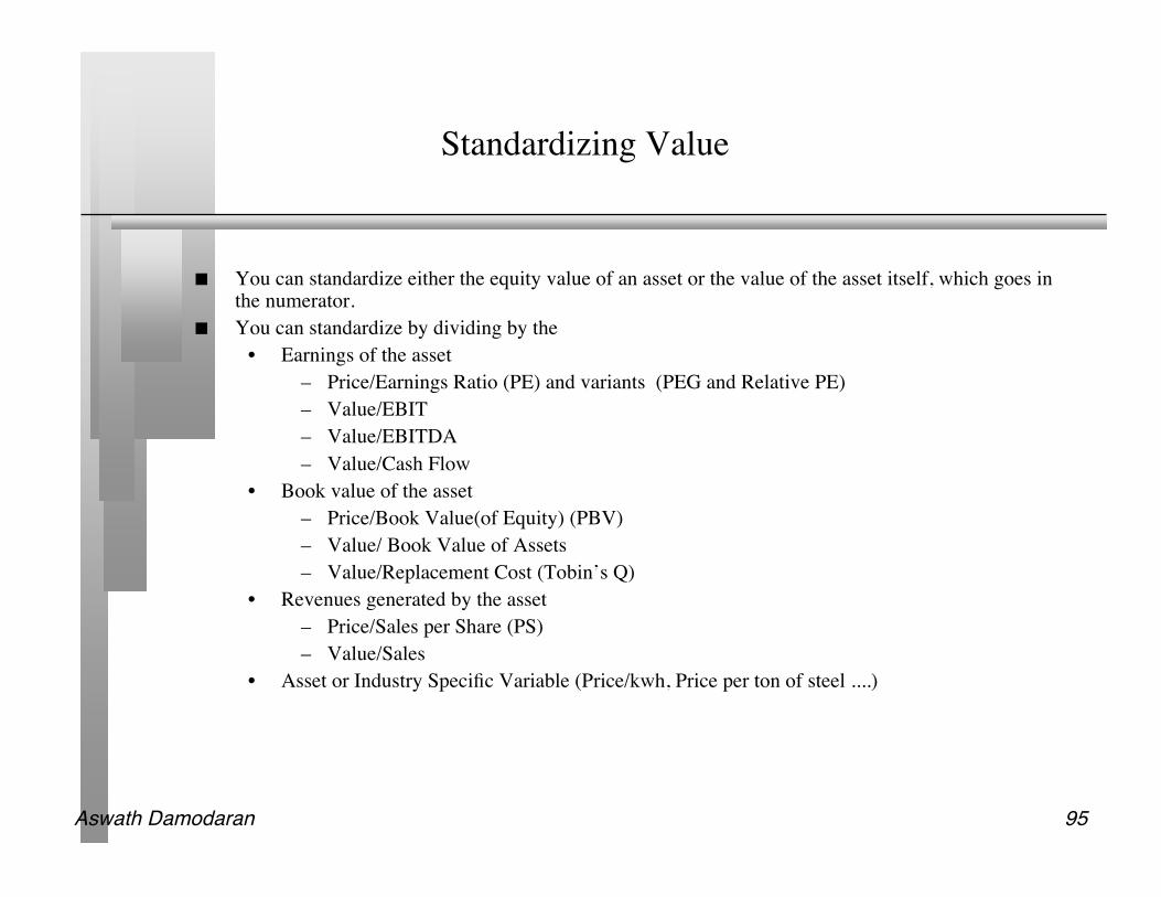
Standardizing Value
You can standardize either the equity value of an asset or the value of the asset itself, which goes inthe numerator.
You can standardize by dividing by the• Earnings of the asset
– Price/Earnings Ratio (PE) and variants (PEG and Relative PE)– Value/EBIT– Value/EBITDA– Value/Cash Flow
• Book value of the asset– Price/Book Value(of Equity) (PBV)– Value/ Book Value of Assets– Value/Replacement Cost (Tobin’s Q)
• Revenues generated by the asset– Price/Sales per Share (PS)– Value/Sales
• Asset or Industry Specific Variable (Price/kwh, Price per ton of steel ....)

Aswath Damodaran 96
The Four Steps to Understanding Multiples
Define the multiple• In use, the same multiple can be defined in different ways by different users. When
comparing and using multiples, estimated by someone else, it is critical that weunderstand how the multiples have been estimated
Describe the multiple• Too many people who use a multiple have no idea what its cross sectional
distribution is. If you do not know what the cross sectional distribution of amultiple is, it is difficult to look at a number and pass judgment on whether it is toohigh or low.
Analyze the multiple• It is critical that we understand the fundamentals that drive each multiple, and the
nature of the relationship between the multiple and each variable. Apply the multiple
• Defining the comparable universe and controlling for differences is far moredifficult in practice than it is in theory.
Aswath Damodaran 97
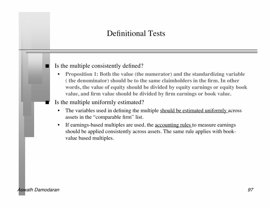
Definitional Tests
Is the multiple consistently defined?• Proposition 1: Both the value (the numerator) and the standardizing variable
( the denominator) should be to the same claimholders in the firm. In otherwords, the value of equity should be divided by equity earnings or equity bookvalue, and firm value should be divided by firm earnings or book value.
Is the multiple uniformly estimated?• The variables used in defining the multiple should be estimated uniformly across
assets in the “comparable firm” list.• If earnings-based multiples are used, the accounting rules to measure earnings
should be applied consistently across assets. The same rule applies with book-value based multiples.

Aswath Damodaran 98
Descriptive Tests
What is the average and standard deviation for this multiple, across theuniverse (market)?
What is the median for this multiple?• The median for this multiple is often a more reliable comparison point.
How large are the outliers to the distribution, and how do we deal with theoutliers?
• Throwing out the outliers may seem like an obvious solution, but if the outliers alllie on one side of the distribution (they usually are large positive numbers), thiscan lead to a biased estimate.
Are there cases where the multiple cannot be estimated? Will ignoring thesecases lead to a biased estimate of the multiple?
How has this multiple changed over time?
Aswath Damodaran 99
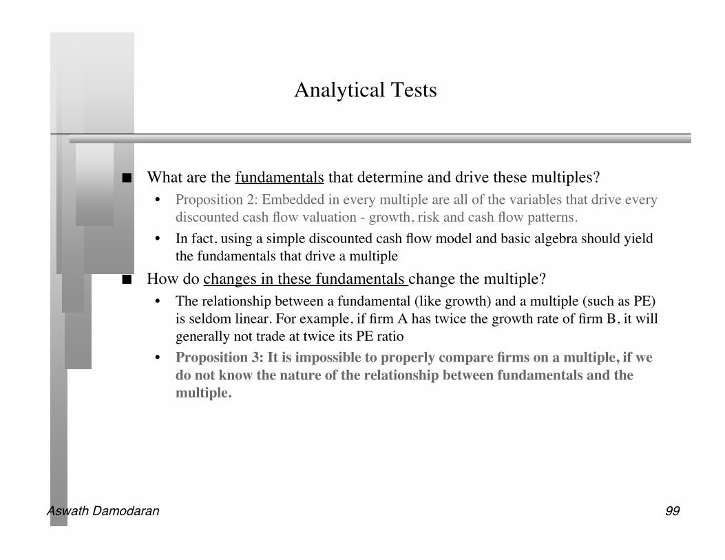
Analytical Tests
What are the fundamentals that determine and drive these multiples?• Proposition 2: Embedded in every multiple are all of the variables that drive every
discounted cash flow valuation - growth, risk and cash flow patterns.• In fact, using a simple discounted cash flow model and basic algebra should yield
the fundamentals that drive a multiple How do changes in these fundamentals change the multiple?
• The relationship between a fundamental (like growth) and a multiple (such as PE)is seldom linear. For example, if firm A has twice the growth rate of firm B, it willgenerally not trade at twice its PE ratio
• Proposition 3: It is impossible to properly compare firms on a multiple, if wedo not know the nature of the relationship between fundamentals and themultiple.

Aswath Damodaran 100
Application Tests
Given the firm that we are valuing, what is a “comparable” firm?• While traditional analysis is built on the premise that firms in the same sector are
comparable firms, valuation theory would suggest that a comparable firm is onewhich is similar to the one being analyzed in terms of fundamentals.
• Proposition 4: There is no reason why a firm cannot be compared withanother firm in a very different business, if the two firms have the same risk,growth and cash flow characteristics.
Given the comparable firms, how do we adjust for differences across firms onthe fundamentals?
• Proposition 5: It is impossible to find an exactly identical firm to the one youare valuing.
Aswath Damodaran 101
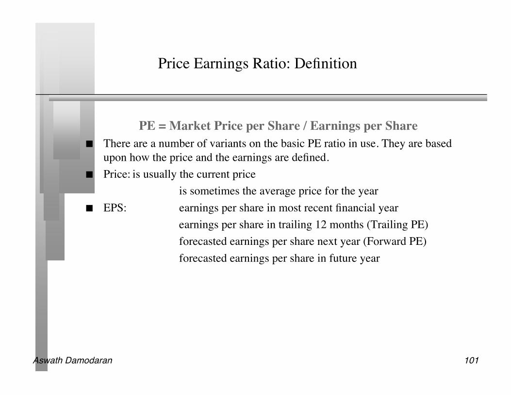
Price Earnings Ratio: Definition
PE = Market Price per Share / Earnings per Share There are a number of variants on the basic PE ratio in use. They are based
upon how the price and the earnings are defined. Price: is usually the current price
is sometimes the average price for the year EPS: earnings per share in most recent financial year
earnings per share in trailing 12 months (Trailing PE)forecasted earnings per share next year (Forward PE)forecasted earnings per share in future year
Aswath Damodaran 102
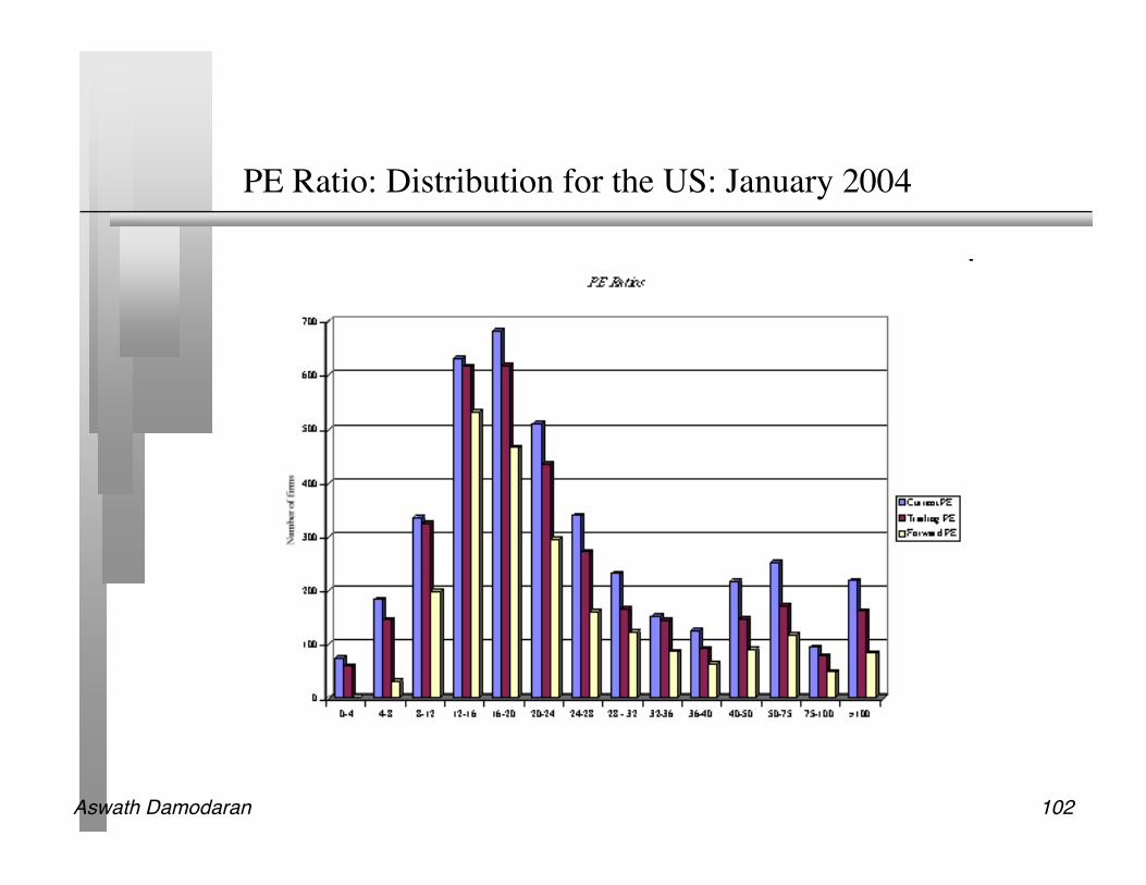
PE Ratio: Distribution for the US: January 2004

Aswath Damodaran 103
PE: Deciphering the Distribution
Current PE Trailing PE Forward PE
Mean 41.41 41.53 30.90
Standard Error 2.42 3.64 1.10
Median 20.76 19.39 19.21
Kurtosis 1062.81 700.63 252.62
Skewness 27.78 24.21 12.48
Minimum 0.40 1.22 2.57
Maximum 6841.25 7184.00 1430.00
Count 4032 3492 2281
500th largest 54.50 43.98 31.13
500th smallest 11.31 11.13 14.29

Aswath Damodaran 104
Comparing PE Ratios: Europe, Japan and Emerging Markets
Median PEJapan = 24.74
US = 20.76Em. Mkts = 18.87
Europe = 15.99

Aswath Damodaran 105
PE Ratio: Germany in September 2004

Aswath Damodaran 106
PE Ratio: Understanding the Fundamentals
To understand the fundamentals, start with a basic equity discounted cashflow model.
With the dividend discount model,
Dividing both sides by the earnings per share,
If this had been a FCFE Model,
P0 =DPS1
r ! gn
P0
EPS0
= PE = Payout Ratio * (1 + gn )
r-gn
P0 =FCFE1
r ! gn
P0
EPS0
= PE = (FCFE/Earnings)* (1 + gn )
r-gn

Aswath Damodaran 107
PE Ratio and Fundamentals
Proposition: Other things held equal, higher growth firms will havehigher PE ratios than lower growth firms.
Proposition: Other things held equal, higher risk firms will have lowerPE ratios than lower risk firms
Proposition: Other things held equal, firms with lower reinvestmentneeds will have higher PE ratios than firms with higher reinvestmentrates.
Of course, other things are difficult to hold equal since high growth firms,tend to have risk and high reinvestment rats.

Aswath Damodaran 108
Using the Fundamental Model to Estimate PE For a HighGrowth Firm
The price-earnings ratio for a high growth firm can also be related tofundamentals. In the special case of the two-stage dividend discount model,this relationship can be made explicit fairly simply:
• For a firm that does not pay what it can afford to in dividends, substituteFCFE/Earnings for the payout ratio.
Dividing both sides by the earnings per share:
P0 =
EPS0 * Payout Ratio *(1+ g)* 1 !(1+ g)
n
(1+ r)n
"
# $ %
&
r - g+
EPS0 * Payout Ration *(1+ g)n *(1+ gn )
(r -gn )(1+ r)n
P0
EPS0
=
Payout Ratio * (1 + g) * 1 !(1 + g)n
(1+ r)n
"
# $ %
& '
r - g+
Payout Ratio n *(1+ g)n * (1 + gn )
(r - gn )(1+ r)n

Aswath Damodaran 109
Expanding the Model
In this model, the PE ratio for a high growth firm is a function of growth, riskand payout, exactly the same variables that it was a function of for the stablegrowth firm.
The only difference is that these inputs have to be estimated for two phases -the high growth phase and the stable growth phase.
Expanding to more than two phases, say the three stage model, will mean thatrisk, growth and cash flow patterns in each stage.
Aswath Damodaran 110
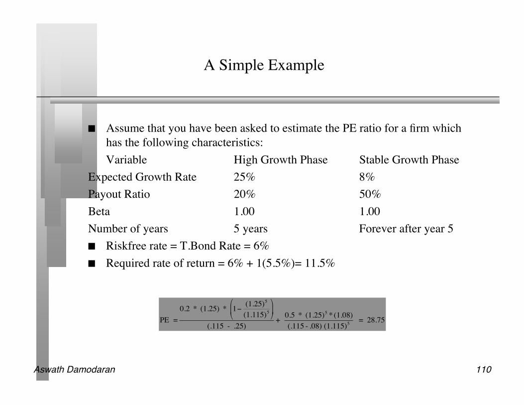
A Simple Example
Assume that you have been asked to estimate the PE ratio for a firm whichhas the following characteristics:Variable High Growth Phase Stable Growth Phase
Expected Growth Rate 25% 8%Payout Ratio 20% 50%Beta 1.00 1.00Number of years 5 years Forever after year 5 Riskfree rate = T.Bond Rate = 6% Required rate of return = 6% + 1(5.5%)= 11.5%
!
PE =
0.2 * (1.25) * 1"(1.25)
5
(1.115)5
#
$ %
&
' (
(.115 - .25)+
0.5 * (1.25)5* (1.08)
(.115 - .08) (1.115)5
= 28.75

Aswath Damodaran 111
PE and Growth: Firm grows at x% for 5 years, 8% thereafter
PE Ratios and Expected Growth: Interest Rate Scenarios
0
20
40
60
80
100
120
140
160
180
5% 10% 15% 20% 25% 30% 35% 40% 45% 50%
Expected Growth Rate
PE
Rati
o r=4%
r=6%
r=8%
r=10%

Aswath Damodaran 112
PE Ratios and Length of High Growth: 25% growth for nyears; 8% thereafter

Aswath Damodaran 113
PE and Risk: Effects of Changing Betas on PE Ratio: Firm with x% growth for 5 years; 8% thereafter
PE Ratios and Beta: Growth Scenarios
0
5
10
15
20
25
30
35
40
45
50
0.75 1.00 1.25 1.50 1.75 2.00
Beta
PE
Rati
o g=25%
g=20%
g=15%
g=8%

Aswath Damodaran 114
PE and Payout

Aswath Damodaran 115
I. Comparisons of PE across time: PE Ratio for the S&P 500

Aswath Damodaran 116
Is low (high) PE cheap (expensive)?
A market strategist argues that stocks are over priced because the PE ratiotoday is too high relative to the average PE ratio across time. Do you agree? Yes No
If you do not agree, what factors might explain the higher PE ratio today?

Aswath Damodaran 117
E/P Ratios , T.Bond Rates and Term Structure

Aswath Damodaran 118
Regression Results
There is a strong positive relationship between E/P ratios and T.Bond rates, asevidenced by the correlation of 0.69 between the two variables.,
In addition, there is evidence that the term structure also affects the PE ratio. In the following regression, using 1960-2003 data, we regress E/P ratios
against the level of T.Bond rates and a term structure variable (T.Bond -T.Bill rate)
E/P = 2.03% + 0.753 T.Bond Rate - 0.355 (T.Bond Rate-T.Bill Rate) (2.19) (6.38) (-1.38)
R squared = 50.85%
Aswath Damodaran 119
II. Comparing PE Ratios across a Sector
Company Name PE Growth
PT Indosat ADR 7.8 0.06
Telebras ADR 8.9 0.075
Telecom Corporation of New Zealand ADR 11.2 0.11
Telecom Argentina Stet - France Telecom SA ADR B 12.5 0.08
Hellenic Telecommunication Organization SA ADR 12.8 0.12
Telecomunicaciones de Chile ADR 16.6 0.08
Swisscom AG ADR 18.3 0.11
Asia Satellite Telecom Holdings ADR 19.6 0.16
Portugal Telecom SA ADR 20.8 0.13
Telefonos de Mexico ADR L 21.1 0.14
Matav RT ADR 21.5 0.22
Telstra ADR 21.7 0.12
Gilat Communications 22.7 0.31
Deutsche Telekom AG ADR 24.6 0.11
British Telecommunications PLC ADR 25.7 0.07
Tele Danmark AS ADR 27 0.09
Telekomunikasi Indonesia ADR 28.4 0.32
Cable & Wireless PLC ADR 29.8 0.14
APT Satellite Holdings ADR 31 0.33
Telefonica SA ADR 32.5 0.18
Royal KPN NV ADR 35.7 0.13
Telecom Italia SPA ADR 42.2 0.14
Nippon Telegraph & Telephone ADR 44.3 0.2
France Telecom SA ADR 45.2 0.19
Korea Telecom ADR 71.3 0.44

Aswath Damodaran 120
PE, Growth and Risk
Dependent variable is: PE
R squared = 66.2% R squared (adjusted) = 63.1%
Variable Coefficient SE t-ratio probConstant 13.1151 3.471 3.78 0.0010Growth rate 121.223 19.27 6.29 ≤ 0.0001Emerging Market -13.8531 3.606 -3.84 0.0009Emerging Market is a dummy: 1 if emerging market
0 if not

Aswath Damodaran 121
Is Telebras under valued?
Predicted PE = 13.12 + 121.22 (.075) - 13.85 (1) = 8.35 At an actual price to earnings ratio of 8.9, Telebras is slightly overvalued.
What about Deutsche Telecom?• If viewed as a developed market telecom13.12 + 121.22 (0.11) -13.85 (0) = 26.45It is slightly undervalued at 24.6 times earnings

Aswath Damodaran 122
Using the entire crosssection: A regression approach
In contrast to the 'comparable firm' approach, the information in the entirecross-section of firms can be used to predict PE ratios.
The simplest way of summarizing this information is with a multipleregression, with the PE ratio as the dependent variable, and proxies for risk,growth and payout forming the independent variables.
Aswath Damodaran 123
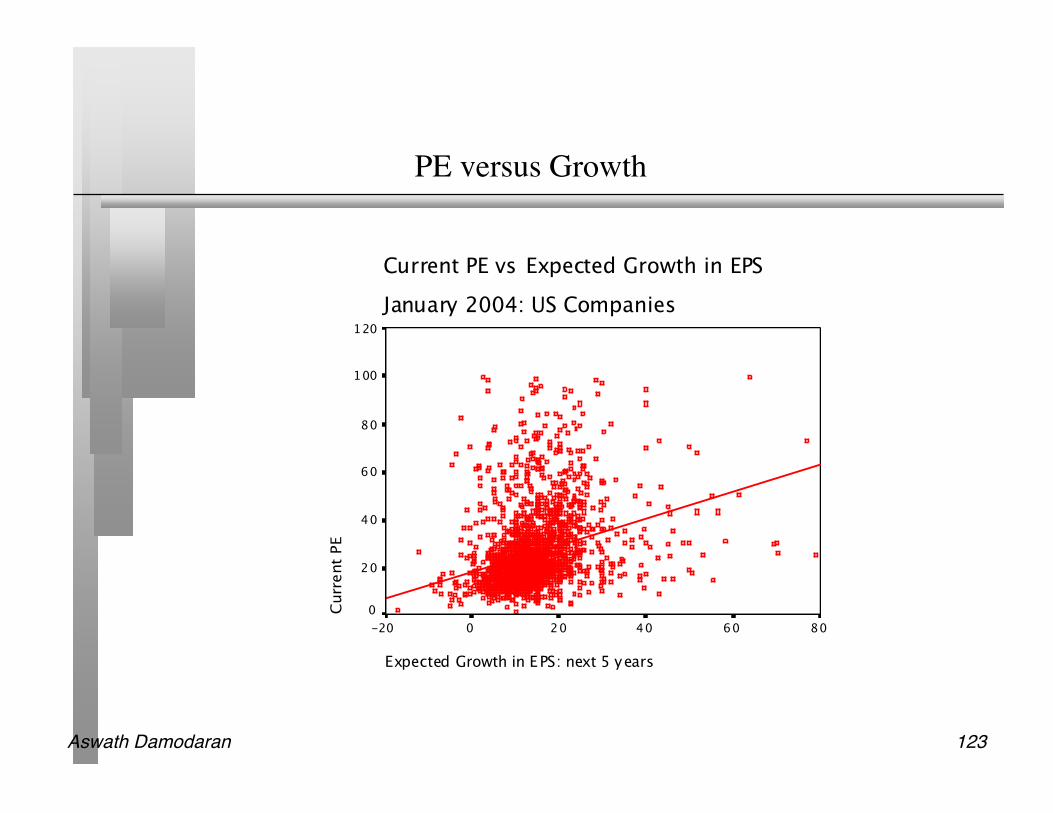
PE versus Growth
Current PE vs Expected Growth in EPS
January 2004: US Companies
Expected Growth in EPS: next 5 years
806040200-20
Curr
ent
PE
120
100
80
60
40
20
0

Aswath Damodaran 124
PE Ratio: Standard Regression for US stocks - January 2004
Model Summary
.467a .218 .217 1049.7506205340
Model
1
R R SquareAdjusted R
SquareStd. Error of the
Estimate
Predictor s: (Constant), PAYOUT, Regression Be ta, ExpectedGrowth in EPS: next 5 years
a.
Coeffici entsa,b
9.475 .961 9.862 .000
.814 .046 .375 17.558 .000
6.283 .437 .298 14.375 .000
6.E-02 .014 .092 4.161 .000
(Constant)
Expected G rowth inEPS: next 5 years
Regression Beta
PAYOUT
Model
1
B Std. Error
UnstandardizedCoefficients
Beta
StandardizedCoefficients
t Sig.
Dependent Variable: Current PEa.
Weighted Least Squares Regression - Weighted by Market Capb.

Aswath Damodaran 125
Problems with the regression methodology
The basic regression assumes a linear relationship between PE ratios and thefinancial proxies, and that might not be appropriate.
The basic relationship between PE ratios and financial variables itself mightnot be stable, and if it shifts from year to year, the predictions from the modelmay not be reliable.
The independent variables are correlated with each other. For example, highgrowth firms tend to have high risk. This multi-collinearity makes thecoefficients of the regressions unreliable and may explain the large changes inthese coefficients from period to period.

Aswath Damodaran 126
The Multicollinearity Problem
Correlations
1 .031 -.325**
. .228 .000
1472 1472 1185
.031 1 -.183**
.228 . .000
1472 6933 4187
-.325** -.183** 1
.000 .000 .
1185 4187 4187
Pearson Correlation
Sig. (2-tailed)
N
Pearson Correlation
Sig. (2-tailed)
N
Pearson Correlation
Sig. (2-tailed)
N
Expected G rowth inRevenues: next 5 year s
Regression Beta
PAYOUT
ExpectedGrowth inRevenues:
next 5 yearsRegression
Beta PAYOUT
Correlation is significant at the 0.01 level (2-tailed).**.
Aswath Damodaran 127
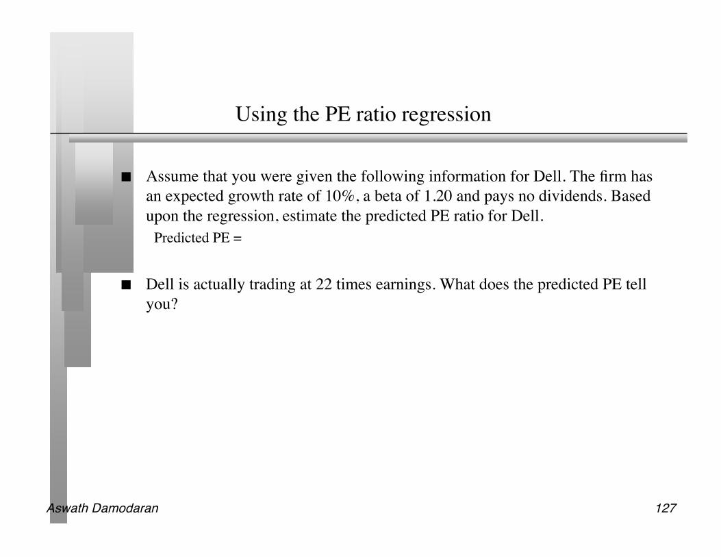
Using the PE ratio regression
Assume that you were given the following information for Dell. The firm hasan expected growth rate of 10%, a beta of 1.20 and pays no dividends. Basedupon the regression, estimate the predicted PE ratio for Dell.
Predicted PE =
Dell is actually trading at 22 times earnings. What does the predicted PE tellyou?
Aswath Damodaran 128
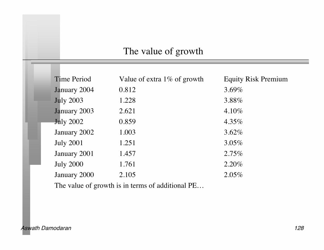
The value of growth
Time Period Value of extra 1% of growth Equity Risk PremiumJanuary 2004 0.812 3.69%July 2003 1.228 3.88%January 2003 2.621 4.10%July 2002 0.859 4.35%January 2002 1.003 3.62%July 2001 1.251 3.05%January 2001 1.457 2.75%July 2000 1.761 2.20%January 2000 2.105 2.05%The value of growth is in terms of additional PE…
Aswath Damodaran 129
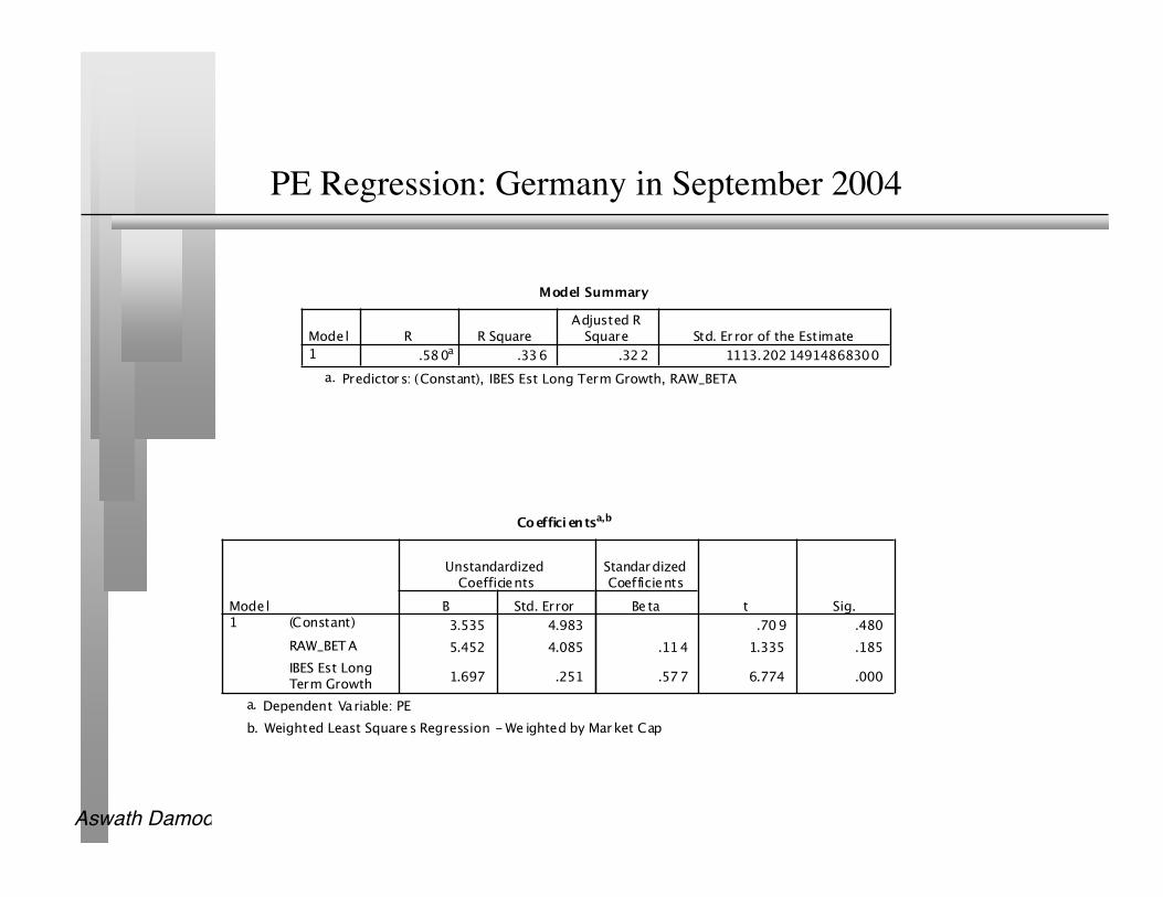
PE Regression: Germany in September 2004
Model Summary
.580a .336 .322 1113.20214914868300
Model
1
R R SquareAdjusted R
Square Std. Er ror of the Estimate
Predictor s: (Constant), IBES Est Long Term Growth, RAW_BETAa.
Coeffici entsa,b
3.535 4.983 .709 .480
5.452 4.085 .114 1.335 .185
1.697 .251 .577 6.774 .000
(Constant)
RAW_BETA
IBES Est LongTerm Growth
Model1
B Std. Error
UnstandardizedCoefficients
Be ta
StandardizedCoefficients
t Sig.
Dependent Variable: PEa.
Weighted Least Squares Regression - We ighted by Market Capb.

Aswath Damodaran 130
Value/Earnings and Value/Cashflow Ratios
While Price earnings ratios look at the market value of equity relative to earnings to equity investors,Value earnings ratios look at the market value of the firm relative to operating earnings. Value tocash flow ratios modify the earnings number to make it a cash flow number.
The form of value to cash flow ratios that has the closest parallels in DCF valuation is the value toFree Cash Flow to the Firm, which is defined as:
Value/FCFF = (Market Value of Equity + Market Value of Debt-Cash)EBIT (1-t) - (Cap Ex - Deprecn) - Chg in WC
Consistency Tests:• If the numerator is net of cash (or if net debt is used, then the interest income from the cash should not be in
denominator• The interest expenses added back to get to EBIT should correspond to the debt in the numerator. If only long
term debt is considered, only long term interest should be added back.

Aswath Damodaran 131
Value of Firm/FCFF: Determinants
Reverting back to a two-stage FCFF DCF model, we get:
• V0 = Value of the firm (today)• FCFF0 = Free Cashflow to the firm in current year• g = Expected growth rate in FCFF in extraordinary growth period (first n years)• WACC = Weighted average cost of capital• gn = Expected growth rate in FCFF in stable growth period (after n years)
V0
=
FCFF0
(1 + g) 1-(1 + g)
n
(1+ WACC)n
!
" #
$
% &
WACC - g +
FCFF0
(1+ g)n
(1+ gn
)
(WACC - gn
)(1 + WACC)n

Aswath Damodaran 132
Value Multiples
Dividing both sides by the FCFF yields,
The value/FCFF multiples is a function of• the cost of capital• the expected growth
V0
FCFF0
=
(1 + g) 1-(1 + g)n
(1 + WACC)n
!
" # $
%
WACC - g +
(1+ g)n (1+ gn )
(WACC - gn )(1 + WACC)n

Aswath Damodaran 133
Value/FCFF Multiples and the Alternatives
Assume that you have computed the value of a firm, using discounted cashflow models. Rank the following multiples in the order of magnitude fromlowest to highest?
Value/EBIT Value/EBIT(1-t) Value/FCFF Value/EBITDA What assumption(s) would you need to make for the Value/EBIT(1-t) ratio to
be equal to the Value/FCFF multiple?

Aswath Damodaran 134
Illustration: Using Value/FCFF Approaches to value a firm:MCI Communications
MCI Communications had earnings before interest and taxes of $3356 millionin 1994 (Its net income after taxes was $855 million).
It had capital expenditures of $2500 million in 1994 and depreciation of$1100 million; Working capital increased by $250 million.
It expects free cashflows to the firm to grow 15% a year for the next five yearsand 5% a year after that.
The cost of capital is 10.50% for the next five years and 10% after that. The company faces a tax rate of 36%.
V0
FCFF0=
(1.15) 1- (1.15)5
(1.105)5
æ
è ç ö
ø
.105 -.15 + (1.15)5(1.05)
(.10 - .05)(1.105)5 = 31.28
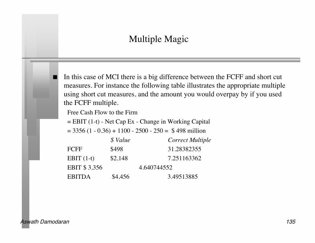
Aswath Damodaran 135
Multiple Magic
In this case of MCI there is a big difference between the FCFF and short cutmeasures. For instance the following table illustrates the appropriate multipleusing short cut measures, and the amount you would overpay by if you usedthe FCFF multiple.
Free Cash Flow to the Firm= EBIT (1-t) - Net Cap Ex - Change in Working Capital= 3356 (1 - 0.36) + 1100 - 2500 - 250 = $ 498 million
$ Value Correct MultipleFCFF $498 31.28382355EBIT (1-t) $2,148 7.251163362EBIT $ 3,356 4.640744552EBITDA $4,456 3.49513885

Aswath Damodaran 136
Reasons for Increased Use of Value/EBITDA
1. The multiple can be computed even for firms that are reporting net losses, since earnings beforeinterest, taxes and depreciation are usually positive.
2. For firms in certain industries, such as cellular, which require a substantial investment in infrastructureand long gestation periods, this multiple seems to be more appropriate than the price/earnings ratio.
3. In leveraged buyouts, where the key factor is cash generated by the firm prior to all discretionaryexpenditures, the EBITDA is the measure of cash flows from operations that can be used to supportdebt payment at least in the short term.
4. By looking at cashflows prior to capital expenditures, it may provide a better estimate of “optimalvalue”, especially if the capital expenditures are unwise or earn substandard returns.
5. By looking at the value of the firm and cashflows to the firm it allows for comparisons across firmswith different financial leverage.

Aswath Damodaran 137
Value/EBITDA Multiple
The Classic Definition
The No-Cash Version
When cash and marketable securities are netted out of value, none of theincome from the cash and securities should be reflected in the denominator.
Value
EBITDA=
Market Value of Equity + Market Value of Debt
Earnings before Interest, Taxes and Depreciation
!
Enterprise Value
EBITDA=
Market Value of Equity + Market Value of Debt - Cash
Earnings before Interest, Taxes and Depreciation
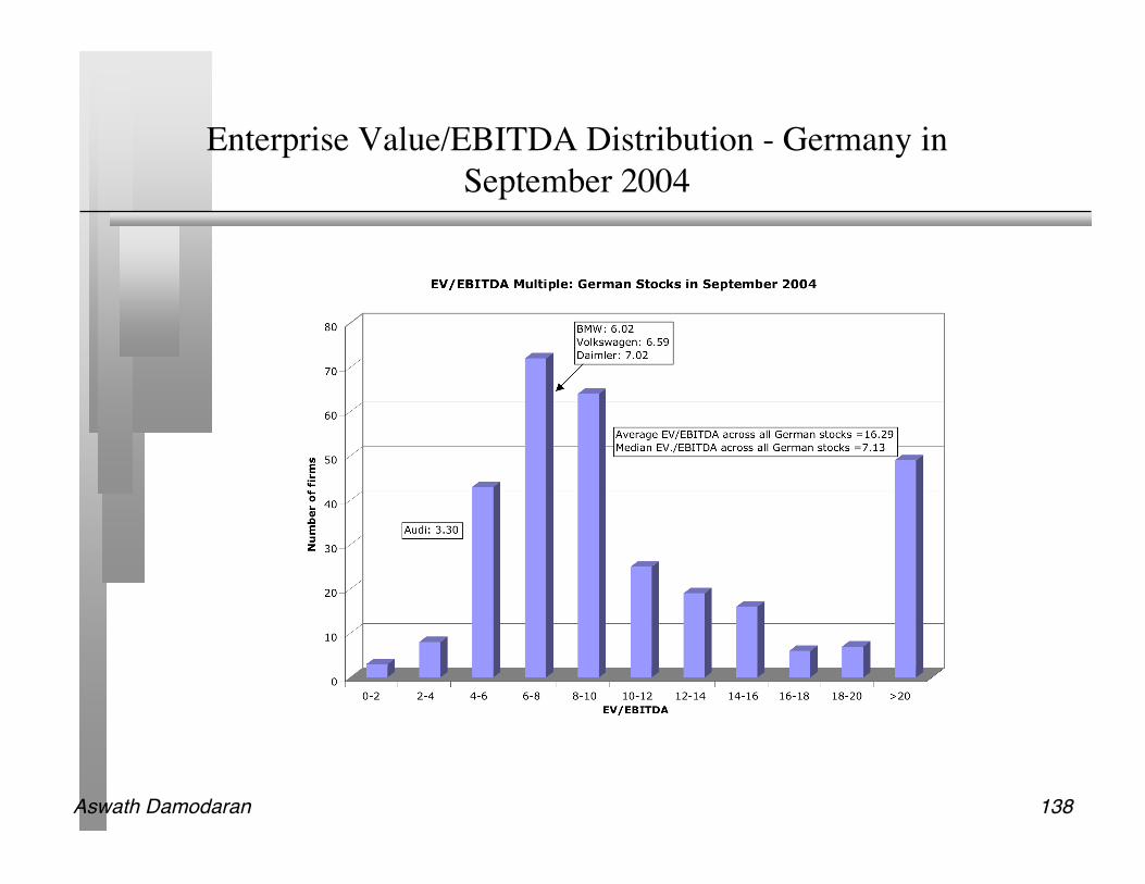
Aswath Damodaran 138
Enterprise Value/EBITDA Distribution - Germany inSeptember 2004

Aswath Damodaran 139
Value/EBITDA Distribution: Rest of the World
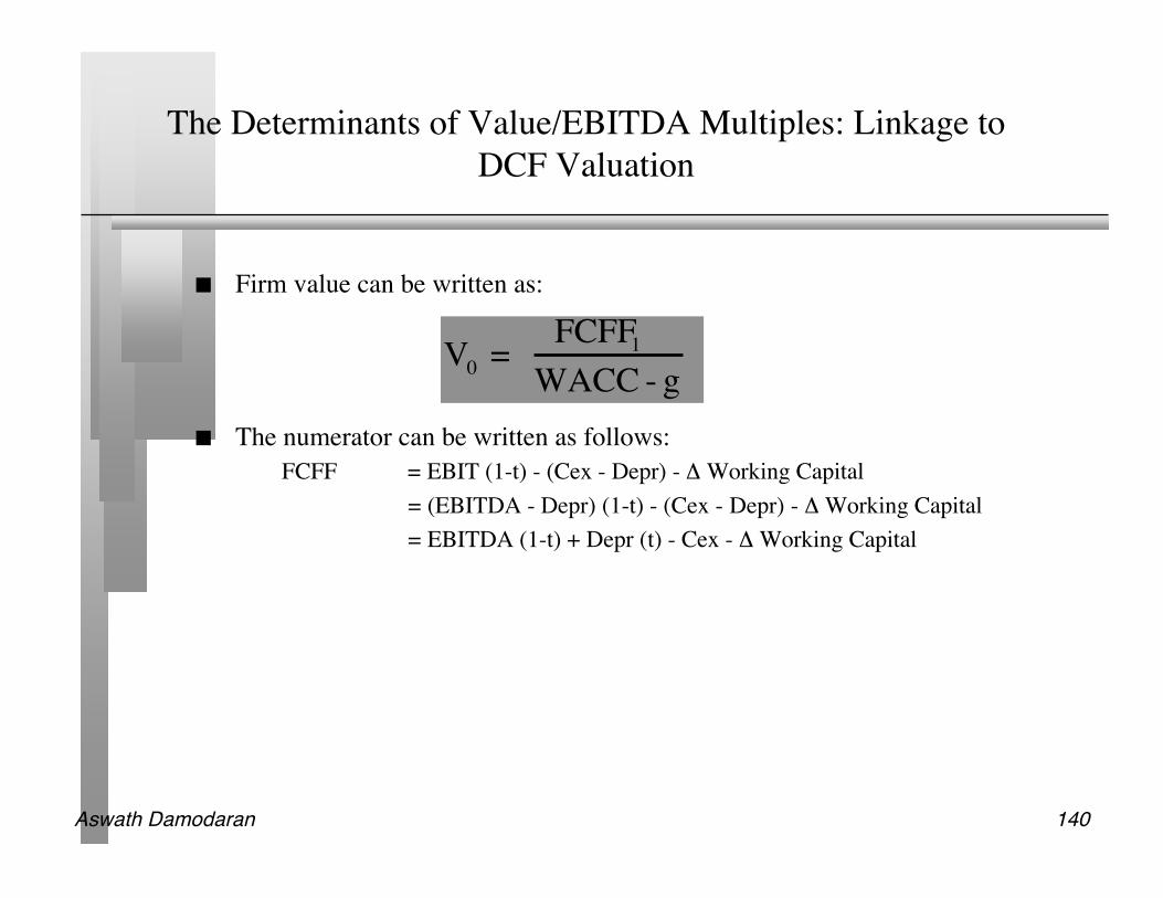
Aswath Damodaran 140
The Determinants of Value/EBITDA Multiples: Linkage toDCF Valuation
Firm value can be written as:
The numerator can be written as follows:FCFF = EBIT (1-t) - (Cex - Depr) - Δ Working Capital
= (EBITDA - Depr) (1-t) - (Cex - Depr) - Δ Working Capital= EBITDA (1-t) + Depr (t) - Cex - Δ Working Capital
V0 = FCFF1
WACC - g

Aswath Damodaran 141
From Firm Value to EBITDA Multiples
Now the Value of the firm can be rewritten as,
Dividing both sides of the equation by EBITDA,
Value = EBITDA (1- t) + Depr (t) - Cex - ! Working Capital
WACC - g
Value
EBITDA =
(1- t)
WACC- g +
Depr (t)/EBITDA
WACC -g -
CEx/EBITDA
WACC - g -
! Working Capital/EBITDA
WACC - g
Aswath Damodaran 142
A Simple Example
Consider a firm with the following characteristics:• Tax Rate = 36%• Capital Expenditures/EBITDA = 30%• Depreciation/EBITDA = 20%• Cost of Capital = 10%• The firm has no working capital requirements• The firm is in stable growth and is expected to grow 5% a year forever.

Aswath Damodaran 143
Calculating Value/EBITDA Multiple
In this case, the Value/EBITDA multiple for this firm can be estimated asfollows:
Value
EBITDA =
(1- .36)
.10 -.05 +
(0.2)(.36)
.10 -.05 -
0.3
.10 - .05 -
0
.10 - .05 = 8.24
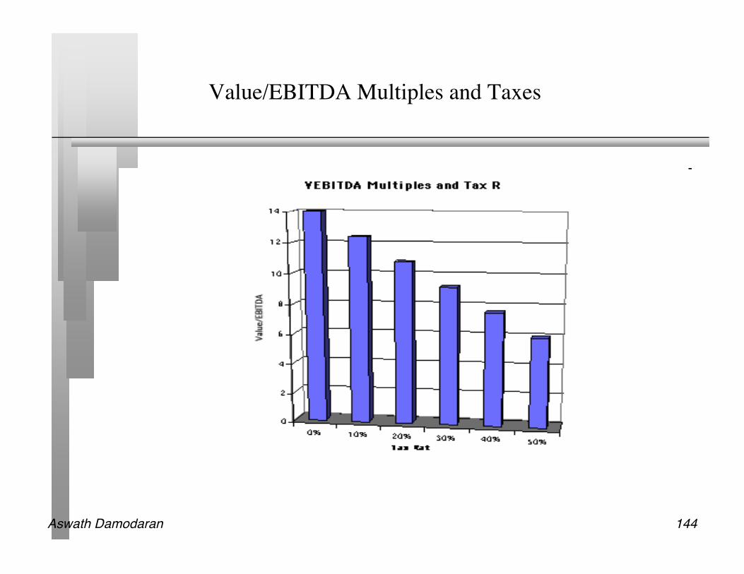
Aswath Damodaran 144
Value/EBITDA Multiples and Taxes
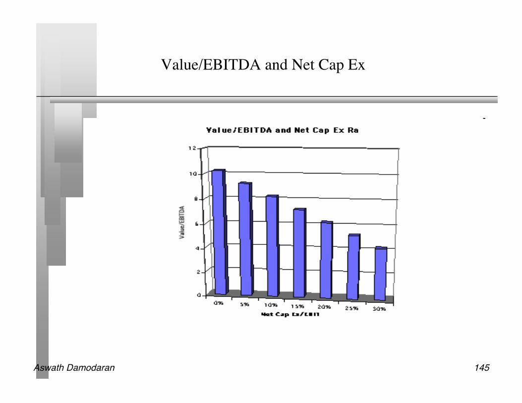
Aswath Damodaran 145
Value/EBITDA and Net Cap Ex

Aswath Damodaran 146
Value/EBITDA Multiples and Return on Capital
Value/EBITDA and Return on Capital
0
2
4
6
8
10
12
6% 7% 8% 9% 10% 11% 12% 13% 14% 15%
Return on Capital
Valu
e/EBIT
DA
WACC=10%
WACC=9%
WACC=8%

Aswath Damodaran 147
Value/EBITDA Multiple: Trucking Companies
Company Name Value EBITDA Value/EBITDAKLLM Trans. Svcs. 114.32$ 48.81$ 2.34Ryder System 5,158.04$ 1,838.26$ 2.81Rollins Truck Leasing 1,368.35$ 447.67$ 3.06Cannon Express Inc. 83.57$ 27.05$ 3.09Hunt (J.B.) 982.67$ 310.22$ 3.17Yellow Corp. 931.47$ 292.82$ 3.18Roadway Express 554.96$ 169.38$ 3.28Marten Transport Ltd. 116.93$ 35.62$ 3.28Kenan Transport Co. 67.66$ 19.44$ 3.48M.S. Carriers 344.93$ 97.85$ 3.53Old Dominion Freight 170.42$ 45.13$ 3.78Trimac Ltd 661.18$ 174.28$ 3.79Matlack Systems 112.42$ 28.94$ 3.88XTRA Corp. 1,708.57$ 427.30$ 4.00Covenant Transport Inc 259.16$ 64.35$ 4.03Builders Transport 221.09$ 51.44$ 4.30Werner Enterprises 844.39$ 196.15$ 4.30Landstar Sys. 422.79$ 95.20$ 4.44AMERCO 1,632.30$ 345.78$ 4.72USA Truck 141.77$ 29.93$ 4.74Frozen Food Express 164.17$ 34.10$ 4.81Arnold Inds. 472.27$ 96.88$ 4.87Greyhound Lines Inc. 437.71$ 89.61$ 4.88USFreightways 983.86$ 198.91$ 4.95Golden Eagle Group Inc. 12.50$ 2.33$ 5.37Arkansas Best 578.78$ 107.15$ 5.40Airlease Ltd. 73.64$ 13.48$ 5.46Celadon Group 182.30$ 32.72$ 5.57Amer. Freightways 716.15$ 120.94$ 5.92Transfinancial Holdings 56.92$ 8.79$ 6.47Vitran Corp. 'A' 140.68$ 21.51$ 6.54Interpool Inc. 1,002.20$ 151.18$ 6.63Intrenet Inc. 70.23$ 10.38$ 6.77Swift Transportation 835.58$ 121.34$ 6.89Landair Services 212.95$ 30.38$ 7.01CNF Transportation 2,700.69$ 366.99$ 7.36Budget Group Inc 1,247.30$ 166.71$ 7.48Caliber System 2,514.99$ 333.13$ 7.55Knight Transportation Inc 269.01$ 28.20$ 9.54Heartland Express 727.50$ 64.62$ 11.26Greyhound CDA Transn Corp 83.25$ 6.99$ 11.91Mark VII 160.45$ 12.96$ 12.38Coach USA Inc 678.38$ 51.76$ 13.11US 1 Inds Inc. 5.60$ (0.17)$ NA
Average 5 .61

Aswath Damodaran 148
A Test on EBITDA
Ryder System looks very cheap on a Value/EBITDA multiple basis, relativeto the rest of the sector. What explanation (other than misvaluation) mightthere be for this difference?

Aswath Damodaran 149
US Market: Cross Sectional RegressionJanuary 2004
Model Summary
.583a
.340 .338 653 .80185507239
Model
1
R R SquareAdjusted R
SquareStd. Er ror of the
Estimate
Predictor s: ( Constant), Reinvestment Rate, Expected Growth
in Revenues: next 5 years, Eff Tax Rat e
a.
Coef fici entsa,b
10.073 .768 13.121 .000
-.152 .022 -.174 -6.878 .000
.907 .039 .563 23.464 .000
-.015 .006 -.062 -2.420 .016
(Constant)
Eff Tax Rate
Expected G rowth inRevenues: next 5 years
Reinvestment Rate
Model
1
B Std. Er ror
UnstandardizedCoefficients
Be ta
StandardizedCoefficients
t Sig.
Dependent Variable: EV/EBITDAa.
Weighted Least Squares Regression - Weighted by Market Capb.
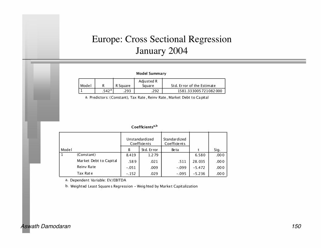
Aswath Damodaran 150
Europe: Cross Sectional RegressionJanuary 2004
Model Summary
.542a .293 .292 1581.333005721082000
Model
1
R R SquareAdjusted R
Square Std. Er ror of the Estimate
Predictors: (Constant), Tax Rate , Reinv Rate , Market Debt to Capitala.
Coefficientsa,b
8.419 1.279 6.580 .000
.589 .021 .511 28.035 .000
-.051 .009 -.099 -5.472 .000
-.152 .029 -.095 -5.236 .000
(Constant)
Market Debt to Capital
Reinv Rate
Tax Rat e
Model
1
B Std. Er ror
UnstandardizedCoefficients
Beta
StandardizedCoefficients
t Sig.
Dependent Variable: EV/EBITDAa.
Weighted Least Squares Regression - Weighted by Market Capitalizationb.

Aswath Damodaran 151
Price-Book Value Ratio: Definition
The price/book value ratio is the ratio of the market value of equity to thebook value of equity, i.e., the measure of shareholders’ equity in the balancesheet.
Price/Book Value = Market Value of EquityBook Value of Equity
Consistency Tests:• If the market value of equity refers to the market value of equity of common stock
outstanding, the book value of common equity should be used in the denominator.• If there is more that one class of common stock outstanding, the market values of
all classes (even the non-traded classes) needs to be factored in.

Aswath Damodaran 152
Price to Book Value: German Stocks in September 2004

Aswath Damodaran 153
Price to Book Value: Europe, Japan and Emerging Markets

Aswath Damodaran 154
Price Book Value Ratio: Stable Growth Firm
Going back to a simple dividend discount model,
Defining the return on equity (ROE) = EPS0 / Book Value of Equity, the valueof equity can be written as:
If the return on equity is based upon expected earnings in the next timeperiod, this can be simplified to,
P0 =DPS1
r ! gn
P 0 = BV0 * ROE * Payout Ratio * (1 + gn )
r-gn
P 0
BV 0
= PBV = ROE * Payout Ratio * (1 + gn )
r-gn
P 0
BV 0
= PBV = ROE * Payout Ratio
r-gn
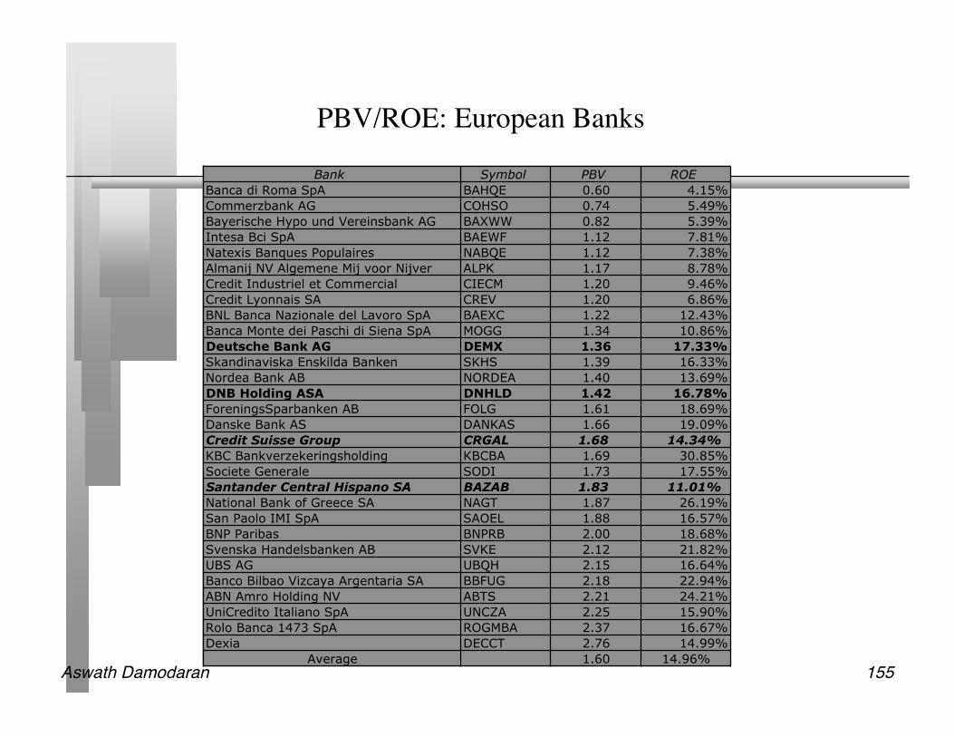
Aswath Damodaran 155
PBV/ROE: European Banks
Bank Symbol PBV ROE
Banca di Roma SpA BAHQE 0.60 4.15%
Commerzbank AG COHSO 0.74 5.49%
Bayerische Hypo und Vereinsbank AG BAXWW 0.82 5.39%
Intesa Bci SpA BAEWF 1.12 7.81%
Natexis Banques Populaires NABQE 1.12 7.38%
Almanij NV Algemene Mij voor Nijver ALPK 1.17 8.78%
Credit Industriel et Commercial CIECM 1.20 9.46%
Credit Lyonnais SA CREV 1.20 6.86%
BNL Banca Nazionale del Lavoro SpA BAEXC 1.22 12.43%
Banca Monte dei Paschi di Siena SpA MOGG 1.34 10.86%
Deutsche Bank AG DEMX 1.36 17.33%
Skandinaviska Enskilda Banken SKHS 1.39 16.33%
Nordea Bank AB NORDEA 1.40 13.69%
DNB Holding ASA DNHLD 1.42 16.78%
ForeningsSparbanken AB FOLG 1.61 18.69%
Danske Bank AS DANKAS 1.66 19.09%
Credit Suisse Group CRGAL 1.68 14.34%
KBC Bankverzekeringsholding KBCBA 1.69 30.85%
Societe Generale SODI 1.73 17.55%
Santander Central Hispano SA BAZAB 1.83 11.01%
National Bank of Greece SA NAGT 1.87 26.19%
San Paolo IMI SpA SAOEL 1.88 16.57%
BNP Paribas BNPRB 2.00 18.68%
Svenska Handelsbanken AB SVKE 2.12 21.82%
UBS AG UBQH 2.15 16.64%
Banco Bilbao Vizcaya Argentaria SA BBFUG 2.18 22.94%
ABN Amro Holding NV ABTS 2.21 24.21%
UniCredito Italiano SpA UNCZA 2.25 15.90%
Rolo Banca 1473 SpA ROGMBA 2.37 16.67%
Dexia DECCT 2.76 14.99%
Average 1.60 14.96%

Aswath Damodaran 156
PBV versus ROE regression
Regressing PBV ratios against ROE for banks yields the following regression:PBV = 0.81 + 5.32 (ROE) R2 = 46%
For every 1% increase in ROE, the PBV ratio should increase by 0.0532.

Aswath Damodaran 157
Under and Over Valued Banks?
Bank Actual Predicted Under or Over
Banca di Roma SpA 0.60 1.03 -41.33%
Commerzbank AG 0.74 1.10 -32.86%
Bayerische Hypo und Vereinsbank AG 0.82 1.09 -24.92%
Intesa Bci SpA 1.12 1.22 -8.51%
Natexis Banques Populaires 1.12 1.20 -6.30%
Almanij NV Algemene Mij voor Nijver 1.17 1.27 -7.82%
Credit Industriel et Commercial 1.20 1.31 -8.30%
Credit Lyonnais SA 1.20 1.17 2.61%
BNL Banca Nazionale del Lavoro SpA 1.22 1.47 -16.71%
Banca Monte dei Paschi di Siena SpA 1.34 1.39 -3.38%
Deutsche Bank AG 1.36 1.73 -21.40%
Skandinaviska Enskilda Banken 1.39 1.68 -17.32%
Nordea Bank AB 1.40 1.54 -9.02%
DNB Holding ASA 1.42 1.70 -16.72%
ForeningsSparbanken AB 1.61 1.80 -10.66%
Danske Bank AS 1.66 1.82 -9.01%
Credit Suisse Group 1.68 1.57 7.20%
KBC Bankverzekeringsholding 1.69 2.45 -30.89%
Societe Generale 1.73 1.74 -0.42%
Santander Central Hispano SA 1.83 1.39 31.37%
National Bank of Greece SA 1.87 2.20 -15.06%
San Paolo IMI SpA 1.88 1.69 11.15%
BNP Paribas 2.00 1.80 11.07%
Svenska Handelsbanken AB 2.12 1.97 7.70%
UBS AG 2.15 1.69 27.17%
Banco Bilbao Vizcaya Argentaria SA 2.18 2.03 7.66%
ABN Amro Holding NV 2.21 2.10 5.23%
UniCredito Italiano SpA 2.25 1.65 36.23%
Rolo Banca 1473 SpA 2.37 1.69 39.74%
Dexia 2.76 1.61 72.04%
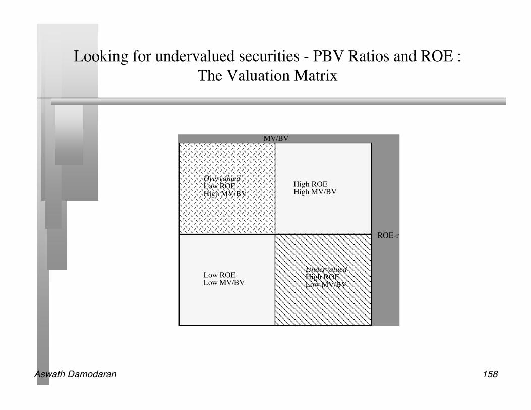
Aswath Damodaran 158
Looking for undervalued securities - PBV Ratios and ROE :The Valuation Matrix
MV/BV
ROE-r
High ROEHigh MV/BV
Low ROELow MV/BV
Overvalued
Low ROEHigh MV/BV
Undervalued
High ROELow MV/BV

Aswath Damodaran 159
Price to Book vs ROE: German Stocks in September 2004
ROE
120100806040200-20
PB
V
10
8
6
4
2
0 Rsq = 0.2355
WAD
US A
SGS
SAH
RAA
PUMLEC
LB R
KOT
KER
GAL
EUX
DEE
DC G
AX3
AQU
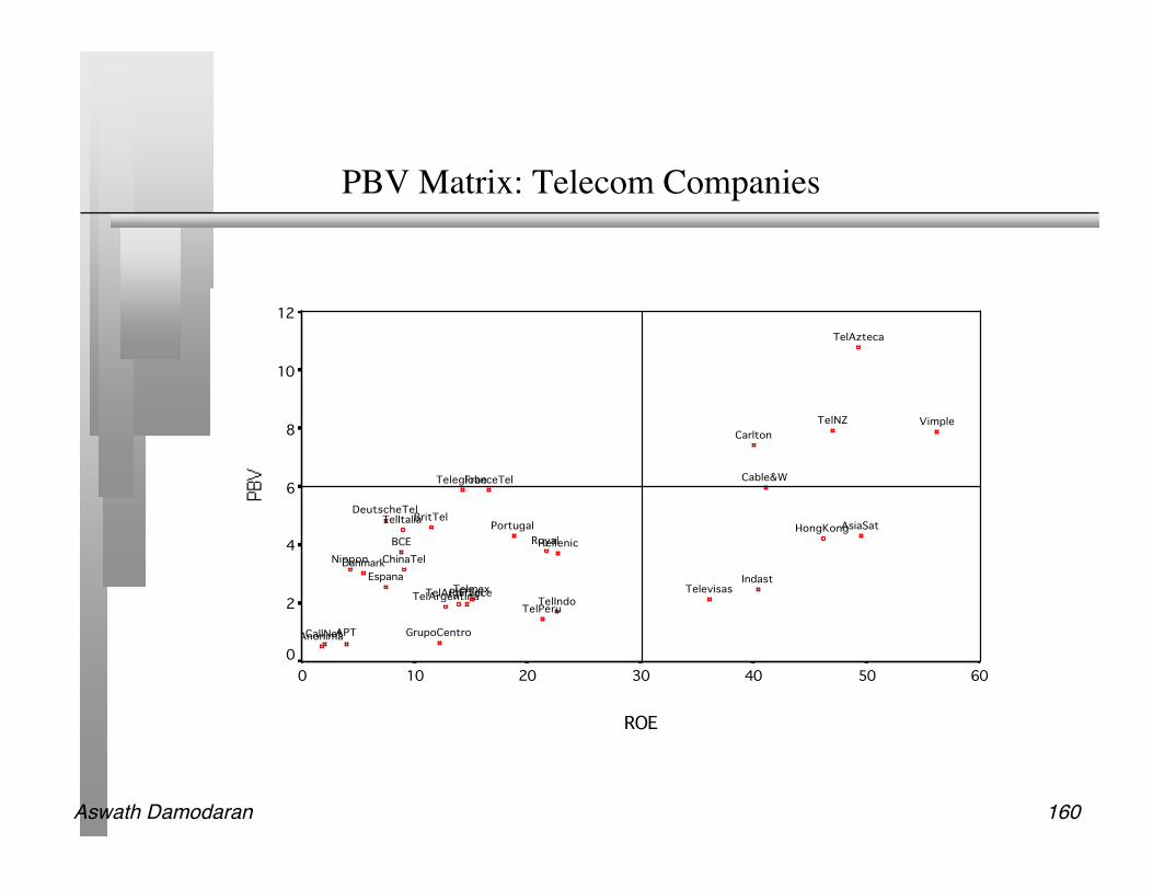
Aswath Damodaran 160
PBV Matrix: Telecom Companies
TelAzteca
TelNZ Vimple
Carlton
Cable&WTeleglobeFranceTel
DeutscheTelBritTelTelItalia
AsiaSatPortugal HongKongRoyalBCE Hellenic
ChinaTelNipponDanmark
Espana IndastTelevisasTelmexTelArgFrancePhilTelTelArgentina TelIndo
TelPeru
GrupoCentroAPTCallNetAnonima
ROE
6050403020100
12
10
8
6
4
2
0
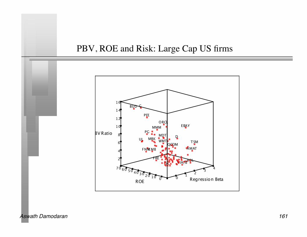
Aswath Damodaran 161
PBV, ROE and Risk: Large Cap US firms
470
PBV Ratio
2
4
TSM
60
6
FNM
ORCL
UL
8
3
BUD
10
AMAT
AOL
50
MRK
12PFE
14
G
PG
16
VIA/B
40
FRE
MMM
SC
2
EBAY
KMB
ROERegression Beta
QCOMWMT
MDT
30
D
120 10 00

Aswath Damodaran 162
IBM: The Rise and Fall and Rise Again
0.00
1.00
2.00
3.00
4.00
5.00
6.00
7.00
8.00
9.00
10.00
1983 1984 1985 1986 1987 1988 1989 1990 1991 1992 1993 1994 1995 1996 1997 1998 1999 2000
Year
Pri
ce t
o B
ook
-40.00%
-30.00%
-20.00%
-10.00%
0.00%
10.00%
20.00%
30.00%
40.00%
50.00%
Ret
urn
on
Eq
uit
y
PBV ROE

Aswath Damodaran 163
PBV Ratio Regression: USJanuary 2004
Model Summary
.943b .889 .889 117.0574933200291
Model
1
R R Squarea
Adjusted RSquare
Std. Er ror of theEstimate
For regression through the origin (the no-intercept model) , RSquare measures the proportion of the variability in thedependent variable about the origin explained by regression.This CANNOT be compared to R Squar e for models whichinclude an intercept.
a.
Predictors: ROE, Regression Beta, PAYOU T, Expected Growth
in EPS: next 5 years
b.
Coeffici entsa,b,c
8.E-02 .004 .256 21.935 .000
2.E-03 .001 .017 1.551 .121
.599 .042 .151 14.249 .000
.140 .003 .628 50.731 .000
Expected G rowth inEPS: next 5 years
PAYOUT
Regression Beta
ROE
Model
1
B Std. Error
UnstandardizedCoefficients
Beta
StandardizedCoefficients
t Sig.
Dependent Variable: PBV Ratioa.
Linear Regression through the Originb.
Weighted Least Squares Regression - Weighted by Market Capc.

Aswath Damodaran 164
PBV Ratio Regression- EuropeJanuary 2004
Model Summary
.830b .689 .689 154.44047748882220
Model
1
R R Squarea
Adjusted RSquare Std. Error of the Estimate
For regression through the origin (the no-intercept model) , R Squaremeasures the propor tion of the variability in the dependent variableabout the origin explained by regression. This CANNOT be comparedto R Square for models which include an inter cept.
a.
Predictors: ROE, Payout Ra tio, B ETAb.
Coefficientsa ,b,c
8.E-03 .002 .074 3.667 .000
1.399 .114 .291 12.279 .000
.104 .004 .537 28.148 .000
Payout Ratio
BETA
ROE
Model
1
B Std. Er ror
UnstandardizedCoefficients
Beta
StandardizedCoefficients
t Sig.
Dependent Variable: PBVa.
Linear Regression through the Originb.
Weighted Least Squares Regression - Weighted by Market Capitalizationc.

Aswath Damodaran 165
Price Sales Ratio: Definition
The price/sales ratio is the ratio of the market value of equity to the sales. Price/ Sales= Market Value of Equity
Total Revenues Consistency Tests
• The price/sales ratio is internally inconsistent, since the market value of equity isdivided by the total revenues of the firm.

Aswath Damodaran 166
Price/Sales Ratio: German Stocks in January 2004

Aswath Damodaran 167
Price to Sales: Europe, Japan and Emerging Markets

Aswath Damodaran 168
Price/Sales Ratio: Determinants
The price/sales ratio of a stable growth firm can be estimated beginning with a2-stage equity valuation model:
Dividing both sides by the sales per share:
P0 =DPS1
r ! gn
P0
Sales0
= PS = Net Profit Margin* Payout Ratio *(1+ gn )
r-gn

Aswath Damodaran 169
PS/Margins: European Retailers - September 2003

Aswath Damodaran 170
Regression Results: PS Ratios and Margins
Regressing PS ratios against net margins,PS = -.39 + 0.6548 (Net Margin) R2 = 43.5%
Thus, a 1% increase in the margin results in an increase of 0.6548 in the pricesales ratios.
The regression also allows us to get predicted PS ratios for these firms
Aswath Damodaran 171
Current versus Predicted Margins
One of the limitations of the analysis we did in these last few pages is thefocus on current margins. Stocks are priced based upon expected marginsrather than current margins.
For most firms, current margins and predicted margins are highly correlated,making the analysis still relevant.
For firms where current margins have little or no correlation with expectedmargins, regressions of price to sales ratios against current margins (or priceto book against current return on equity) will not provide much explanatorypower.
In these cases, it makes more sense to run the regression using eitherpredicted margins or some proxy for predicted margins.

Aswath Damodaran 172
A Case Study: The Internet Stocks
ROWEGSVIPPODTURF BUYX ELTXGEEKRMIIFATB TMNTONEM ABTL INFO ANETITRAIIXLBIZZ EGRPACOMALOYBIDSSPLN EDGRPSIX ATHY AMZN
CLKS PCLNAPNT SONENETO
CBIS NTPACSGPINTW RAMP
DCLKCNETATHMMQST FFIV
SCNT MMXIINTM
SPYGLCOS
PKSI
-0
10
20
30
-0.8 -0.6 -0.4 -0.2
AdjMargin
AdjPS
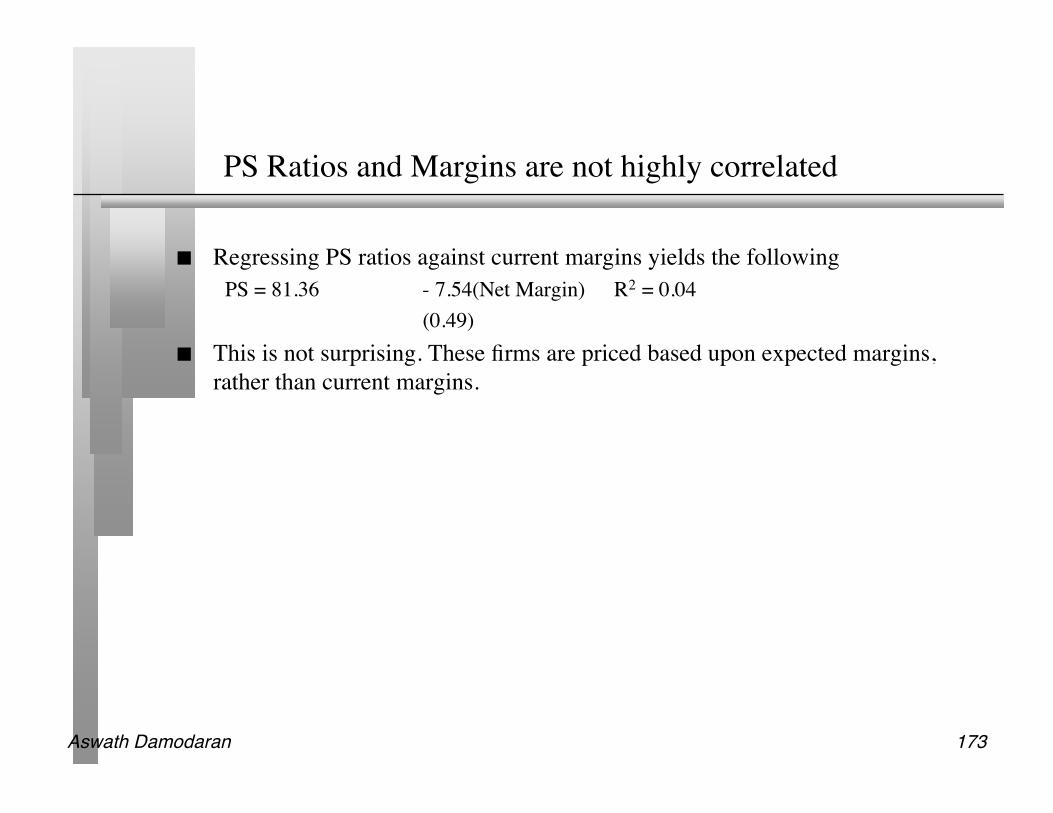
Aswath Damodaran 173
PS Ratios and Margins are not highly correlated
Regressing PS ratios against current margins yields the followingPS = 81.36 - 7.54(Net Margin) R2 = 0.04
(0.49) This is not surprising. These firms are priced based upon expected margins,
rather than current margins.
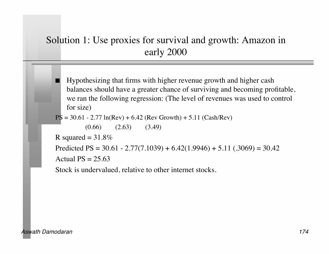
Aswath Damodaran 174
Solution 1: Use proxies for survival and growth: Amazon inearly 2000
Hypothesizing that firms with higher revenue growth and higher cashbalances should have a greater chance of surviving and becoming profitable,we ran the following regression: (The level of revenues was used to controlfor size)
PS = 30.61 - 2.77 ln(Rev) + 6.42 (Rev Growth) + 5.11 (Cash/Rev)(0.66) (2.63) (3.49)
R squared = 31.8%Predicted PS = 30.61 - 2.77(7.1039) + 6.42(1.9946) + 5.11 (.3069) = 30.42Actual PS = 25.63Stock is undervalued, relative to other internet stocks.

Aswath Damodaran 175
Solution 2: Use forward multiples
Global Crossing lost $1.9 billion in 2001 and is expected to continue to lose money forthe next 3 years. In a discounted cashflow valuation (see notes on DCF valuation) ofGlobal Crossing, we estimated an expected EBITDA for Global Crossing in five yearsof $ 1,371 million.
The average enterprise value/ EBITDA multiple for healthy telecomm firms is 7.2currently.
Applying this multiple to Global Crossing’s EBITDA in year 5, yields a value in year 5of
• Enterprise Value in year 5 = 1371 * 7.2 = $9,871 million• Enterprise Value today = $ 9,871 million/ 1.1385 = $5,172 million(The cost of capital for Global Crossing is 13.80%)• The probability that Global Crossing will not make it as a going concern is 77%.• Expected Enterprise value today = 0.23 (5172) = $1,190 million

Aswath Damodaran 176
PS Regression: United States - January 2004Model Summary
.932b .869 .868 114.30566982647230
Model
1
R R Squarea
Adjusted RSquare
Std. Error of theEstimate
For regression through the origin (the no-intercept model) , RSquare measures the proport ion of the variability in thedependent variable about the origin explained by regression.This CANNOT be compared to R Square for models whichinclude an intercept.
a.
Predictors: Net Margin, Regression Beta, PAYOUT, Expected
Growth in EPS: next 5 years
b.
Coeffici entsa,b,c
4.E-02 .004 .136 10.195 .000
-.011 .001 -.110 -9.425 .000
.549 .043 .156 12.658 .000
.234 .004 .799 59.926 .000
Expected G rowth inEPS: next 5 years
PAYOUT
Regression Beta
Net Margin
Model
1
B Std. Error
UnstandardizedCoefficients
Beta
StandardizedCoefficients
t Sig.
Dependent Variable: PS_RATIOa.
Linear Regression through the Originb.
Weighted Least Squares Regression - Weighted by Market Capc.

Aswath Damodaran 177
PS Regression: Europe in January 2004
Model Summary
.757b .574 .573 134.938678072015
Model
1
R R Squarea
Adjusted RSquare
Std. Error of theEstimate
For regression through the origin (the no-intercept model) ,R Square measures the proportion of the variab ility in thedependent variable about the origin explained byregression. This CANNOT be compar ed to R Square for
models which include an intercept.
a.
Predictors: Net Mar gin, Payout Ratio, BETAb.
Coefficientsa ,b,c
5.E-03 .002 .065 2.777 .006
.937 .095 .261 9.909 .000
.110 .004 .516 26.153 .000
Payout Ratio
BETA
Net Margin
Model
1
B Std. Er ror
UnstandardizedCoefficients
Beta
StandardizedCoefficients
t Sig.
Dependent Variable: PSa.
Linear Regression through the Originb.
Weighted Least Squares Regression - Weighted by Market Capitalizationc.

Aswath Damodaran 178
Choosing Between the Multiples
As presented in this section, there are dozens of multiples that can bepotentially used to value an individual firm.
In addition, relative valuation can be relative to a sector (or comparable firms)or to the entire market (using the regressions, for instance)
Since there can be only one final estimate of value, there are three choices atthis stage:
• Use a simple average of the valuations obtained using a number of differentmultiples
• Use a weighted average of the valuations obtained using a nmber of differentmultiples
• Choose one of the multiples and base your valuation on that multiple

Aswath Damodaran 179
Picking one Multiple
This is usually the best way to approach this issue. While a range of valuescan be obtained from a number of multiples, the “best estimate” value isobtained using one multiple.
The multiple that is used can be chosen in one of two ways:• Use the multiple that best fits your objective. Thus, if you want the company to be
undervalued, you pick the multiple that yields the highest value.• Use the multiple that has the highest R-squared in the sector when regressed
against fundamentals. Thus, if you have tried PE, PBV, PS, etc. and runregressions of these multiples against fundamentals, use the multiple that worksbest at explaining differences across firms in that sector.
• Use the multiple that seems to make the most sense for that sector, given howvalue is measured and created.
Aswath Damodaran 180
A More Intuitive Approach
Managers in every sector tend to focus on specific variables when analyzingstrategy and performance. The multiple used will generally reflect this focus.Consider three examples.
• In retailing: The focus is usually on same store sales (turnover) and profit margins.Not surprisingly, the revenue multiple is most common in this sector.
• In financial services: The emphasis is usually on return on equity. Book Equity isoften viewed as a scarce resource, since capital ratios are based upon it. Price tobook ratios dominate.
• In technology: Growth is usually the dominant theme. PEG ratios were invented inthis sector.

Aswath Damodaran 181
In Practice…
As a general rule of thumb, the following table provides a way of picking amultiple for a sector
Sector Multiple Used RationaleCyclical Manufacturing PE, Relative PE Often with normalized earningsHigh Tech, High Growth PEG Big differences in growth across
firmsHigh Growth/No Earnings PS, VS Assume future margins will be goodHeavy Infrastructure VEBITDA Firms in sector have losses in early
years and reported earnings can varydepending on depreciation method
REITa P/CF Generally no cap ex investments from equity earnings
Financial Services PBV Book value often marked to marketRetailing PS If leverage is similar across firms
VS If leverage is different

Aswath Damodaran 182
Reviewing: The Four Steps to Understanding Multiples
Define the multiple• Check for consistency• Make sure that they are estimated uniformly
Describe the multiple• Multiples have skewed distributions: The averages are seldom good indicators of
typical multiples• Check for bias, if the multiple cannot be estimated
Analyze the multiple• Identify the companion variable that drives the multiple• Examine the nature of the relationship
Apply the multiple

Aswath Damodaran 183
Real Options: Fact and Fantasy
Aswath Damodaran
Aswath Damodaran 184
Underlying Theme: Searching for an Elusive Premium
Traditional discounted cashflow models under estimate the value ofinvestments, where there are options embedded in the investments to
• Delay or defer making the investment (delay)• Adjust or alter production schedules as price changes (flexibility)• Expand into new markets or products at later stages in the process, based upon
observing favorable outcomes at the early stages (expansion)• Stop production or abandon investments if the outcomes are unfavorable at early
stages (abandonment) Put another way, real option advocates believe that you should be paying a
premium on discounted cashflow value estimates.

Aswath Damodaran 185
Three Basic Questions
When is there a real option embedded in a decision or an asset? When does that real option have significant economic value? Can that value be estimated using an option pricing model?

Aswath Damodaran 186
When is there an option embedded in an action?
An option provides the holder with the right to buy or sell a specifiedquantity of an underlying asset at a fixed price (called a strike price or anexercise price) at or before the expiration date of the option.
There has to be a clearly defined underlying asset whose value changes overtime in unpredictable ways.
The payoffs on this asset (real option) have to be contingent on an specifiedevent occurring within a finite period.

Aswath Damodaran 187
Payoff Diagram on a Call
Price of underlying asset
StrikePrice
Net Payoff on Call

Aswath Damodaran 188
Example 1: Product Patent as an Option
Present Value of Expected Cash Flows on Product
PV of Cash Flows from Project
Initial Investment in Project
Project has negativeNPV in this section
Project's NPV turns positive in this section

Aswath Damodaran 189
Example 2: Undeveloped Oil Reserve as an option
Value of estimated reserveof natural resource
Net Payoff onExtraction
Cost of Developing Reserve

Aswath Damodaran 190
Example 3: Expansion of existing project as an option
Present Value of Expected Cash Flows on Expansion
PV of Cash Flows from Expansion
Additional Investment to Expand
Firm will not expand inthis section
Expansion becomes attractive in this section
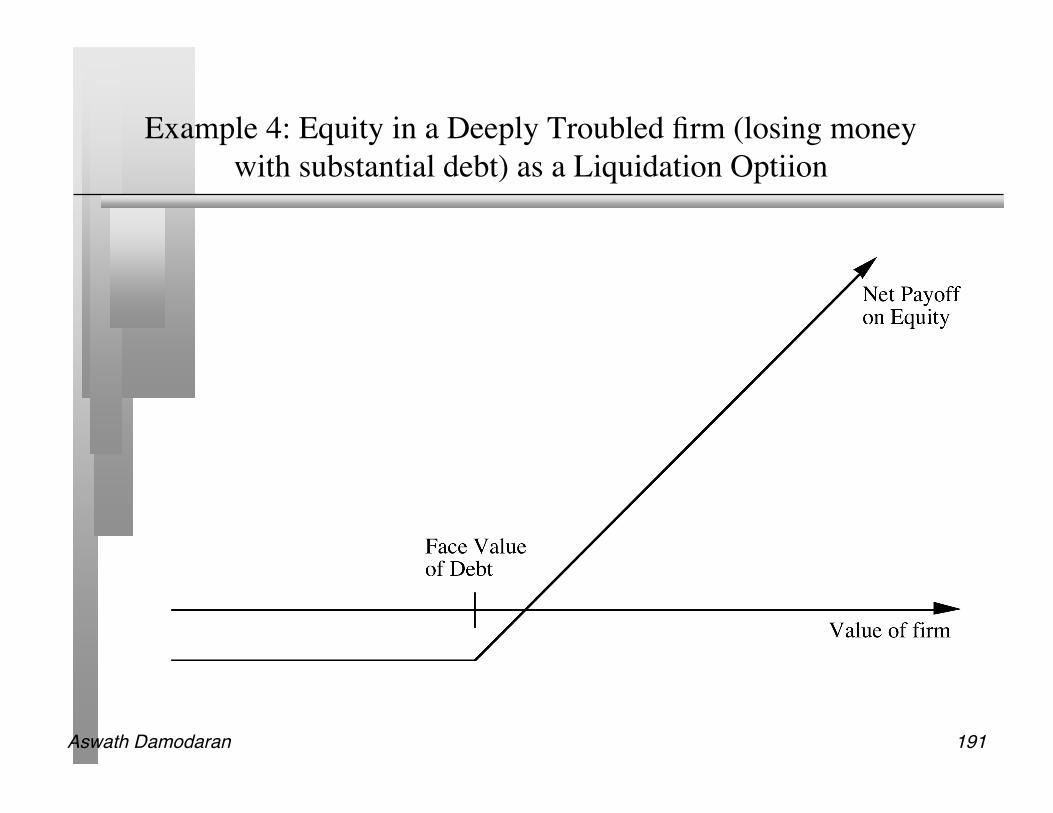
Aswath Damodaran 191
Example 4: Equity in a Deeply Troubled firm (losing moneywith substantial debt) as a Liquidation Optiion

Aswath Damodaran 192
When does the option have significant economic value?
For an option to have significant economic value, there has to be a restrictionon competition in the event of the contingency. In a perfectly competitiveproduct market, no contingency, no matter how positive, will generatepositive net present value.
At the limit, real options are most valuable when you have exclusivity - youand only you can take advantage of the contingency. They become lessvaluable as the barriers to competition become less steep.
Aswath Damodaran 193
Exclusivity: Putting Real Options to the Test
Product Options: Patent on a drug• Patents restrict competitors from developing similar products• Patents do not restrict competitors from developing other products to treat the
same disease. Natural Resource options: An undeveloped oil reserve or gold mine.
• Natural resource reserves are limited.• It takes time and resources to develop new reserves
Growth Options: Expansion into a new product or market• Barriers may range from strong (exclusive licenses granted by the government - as
in telecom businesses) to weaker (brand name, knowledge of the market) toweakest (first mover).
Equity in a Deeply Troubled Firm as a Liquidation Option• Option value greatest when equity investors have the exclusive power to decide on
whether to liquidate or not• Option value is reduced if lenders or the court get some or much of the power.
Aswath Damodaran 194
Determinants of option value
Variables Relating to Underlying Asset• Value of Underlying Asset; as this value increases, the right to buy at a fixed price (calls) will
become more valuable and the right to sell at a fixed price (puts) will become less valuable.• Variance in that value; as the variance increases, both calls and puts will become more
valuable because all options have limited downside and depend upon price volatility for upside.• Expected dividends on the asset, which are likely to reduce the price appreciation component
of the asset, reducing the value of calls and increasing the value of puts. Variables Relating to Option
• Strike Price of Options; the right to buy (sell) at a fixed price becomes more (less) valuable at alower price.
• Life of the Option; both calls and puts benefit from a longer life. Level of Interest Rates; as rates increase, the right to buy (sell) at a fixed price in the
future becomes more (less) valuable.

Aswath Damodaran 195
When can you use an option pricing model to value a realoption?
All option pricing models are built on the premise of replication and arbitrage. Replication: The objective in creating a replicating portfolio is to use a
combination of riskfree borrowing/lending and the underlying asset to createthe same cashflows as the option being valued.
• Call = Borrowing + Buying D of the Underlying Stock• Put = Selling Short D on Underlying Asset + Lending• The number of shares bought or sold is called the option delta.
Arbitrage: If two assets have the same cashflows, they cannot sell at differentprices. If they do, the principles of arbitrage then apply, and the value of theoption has to be equal to the value of the replicating portfolio.
Aswath Damodaran 196
The Black Scholes Model
Value of call = S N (d1) - K e-rt N(d2)where,
• d2 = d1 - σ √t The replicating portfolio is embedded in the Black-Scholes model. To
replicate this call, you would need to• Buy N(d1) shares of stock; N(d1) is called the option delta• Borrow K e-rt N(d2)
d1 =
lnS
K
! "
# $ + (r +
% 2
2) t
% t
Aswath Damodaran 197
The Normal Distributiond N(d) d N(d) d N(d)
-3.00 0.0013 -1.00 0.1587 1.05 0.8531
-2.95 0.0016 -0.95 0.1711 1.10 0.8643
-2.90 0.0019 -0.90 0.1841 1.15 0.8749
-2.85 0.0022 -0.85 0.1977 1.20 0.8849
-2.80 0.0026 -0.80 0.2119 1.25 0.8944
-2.75 0.0030 -0.75 0.2266 1.30 0.9032
-2.70 0.0035 -0.70 0.2420 1.35 0.9115
-2.65 0.0040 -0.65 0.2578 1.40 0.9192
-2.60 0.0047 -0.60 0.2743 1.45 0.9265
-2.55 0.0054 -0.55 0.2912 1.50 0.9332
-2.50 0.0062 -0.50 0.3085 1.55 0.9394
-2.45 0.0071 -0.45 0.3264 1.60 0.9452
-2.40 0.0082 -0.40 0.3446 1.65 0.9505
-2.35 0.0094 -0.35 0.3632 1.70 0.9554
-2.30 0.0107 -0.30 0.3821 1.75 0.9599
-2.25 0.0122 -0.25 0.4013 1.80 0.9641
-2.20 0.0139 -0.20 0.4207 1.85 0.9678
-2.15 0.0158 -0.15 0.4404 1.90 0.9713
-2.10 0.0179 -0.10 0.4602 1.95 0.9744
-2.05 0.0202 -0.05 0.4801 2.00 0.9772
-2.00 0.0228 0.00 0.5000 2.05 0.9798
-1.95 0.0256 0.05 0.5199 2.10 0.9821
-1.90 0.0287 0.10 0.5398 2.15 0.9842
-1.85 0.0322 0.15 0.5596 2.20 0.9861
-1.80 0.0359 0.20 0.5793 2.25 0.9878
-1.75 0.0401 0.25 0.5987 2.30 0.9893
-1.70 0.0446 0.30 0.6179 2.35 0.9906
-1.65 0.0495 0.35 0.6368 2.40 0.9918
-1.60 0.0548 0.40 0.6554 2.45 0.9929
-1.55 0.0606 0.45 0.6736 2.50 0.9938
-1.50 0.0668 0.50 0.6915 2.55 0.9946
-1.45 0.0735 0.55 0.7088 2.60 0.9953
-1.40 0.0808 0.60 0.7257 2.65 0.9960
-1.35 0.0885 0.65 0.7422 2.70 0.9965
-1.30 0.0968 0.70 0.7580 2.75 0.9970
-1.25 0.1056 0.75 0.7734 2.80 0.9974
-1.20 0.1151 0.80 0.7881 2.85 0.9978
-1.15 0.1251 0.85 0.8023 2.90 0.9981
-1.10 0.1357 0.90 0.8159 2.95 0.9984
-1.05 0.1469 0.95 0.8289 3.00 0.9987
-1.00 0.1587 1.00 0.8413
d1
N(d1)

Aswath Damodaran 198
Adjusting for Dividends
If the dividend yield (y = dividends/ Current value of the asset) of theunderlying asset is expected to remain unchanged during the life of theoption, the Black-Scholes model can be modified to take dividends intoaccount.C = S e-yt N(d1) - K e-rt N(d2)
where,
d2 = d1 - σ √t The value of a put can also be derived:
P = K e-rt (1-N(d2)) - S e-yt (1-N(d1))
d1 =
lnS
K
! "
# $ + (r - y +
%2
2) t
% t

Aswath Damodaran 199
Example 1: Valuing a Product Patent as an option: Avonex
Biogen, a bio-technology firm, has a patent on Avonex, a drug to treatmultiple sclerosis, for the next 17 years, and it plans to produce and sell thedrug by itself. The key inputs on the drug are as follows:
PV of Cash Flows from Introducing the Drug Now = S = $ 3.422 billionPV of Cost of Developing Drug for Commercial Use = K = $ 2.875 billionPatent Life = t = 17 years Riskless Rate = r = 6.7% (17-year T.Bond rate)Variance in Expected Present Values =s2 = 0.224 (Industry average firm variance for
bio-tech firms)Expected Cost of Delay = y = 1/17 = 5.89%d1 = 1.1362 N(d1) = 0.8720d2 = -0.8512 N(d2) = 0.2076
Call Value= 3,422 exp(-0.0589)(17) (0.8720) - 2,875 (exp(-0.067)(17) (0.2076)= $ 907million

Aswath Damodaran 200
Valuing a firm with patents
The value of a firm with a substantial number of patents can be derived usingthe option pricing model.
Value of Firm = Value of commercial products (using DCF value+ Value of existing patents (using option pricing)+ (Value of New patents that will be obtained in the future – Cost of obtaining these patents)
The last input measures the efficiency of the firm in converting its R&D intocommercial products. If we assume that a firm earns its cost of capital fromresearch, this term will become zero.
If we use this approach, we should be careful not to double count and allowfor a high growth rate in cash flows (in the DCF valuation).

Aswath Damodaran 201
Value of Biogen’s existing products
· Biogen had two commercial products (a drug to treat Hepatitis B and Intron)at the time of this valuation that it had licensed to other pharmaceutical firms.
· The license fees on these products were expected to generate $ 50 million inafter-tax cash flows each year for the next 12 years. To value these cashflows, which were guaranteed contractually, the pre-tax cost of debt of theguarantors (6.7%) was used:
Present Value of License Fees = $ 50 million (1 – (1.067)-12)/.067= $ 403.56 million
Aswath Damodaran 202
Value of Biogen’s Future R&D
· Biogen continued to fund research into new products, spending about $ 100million on R&D in the most recent year. These R&D expenses were expectedto grow 20% a year for the next 10 years, and 5% thereafter.
· It was assumed that every dollar invested in research would create $ 1.25 invalue in patents (valued using the option pricing model described above) forthe next 10 years, and break even after that (i.e., generate $ 1 in patent valuefor every $ 1 invested in R&D).
· There was a significant amount of risk associated with this component and thecost of capital was estimated to be 15%.
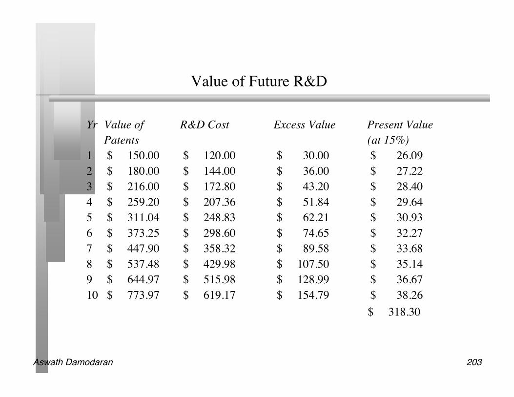
Aswath Damodaran 203
Value of Future R&D
Yr Value of R&D Cost Excess Value Present ValuePatents (at 15%)
1 $ 150.00 $ 120.00 $ 30.00 $ 26.09 2 $ 180.00 $ 144.00 $ 36.00 $ 27.22 3 $ 216.00 $ 172.80 $ 43.20 $ 28.40 4 $ 259.20 $ 207.36 $ 51.84 $ 29.64 5 $ 311.04 $ 248.83 $ 62.21 $ 30.93 6 $ 373.25 $ 298.60 $ 74.65 $ 32.27 7 $ 447.90 $ 358.32 $ 89.58 $ 33.68 8 $ 537.48 $ 429.98 $ 107.50 $ 35.14 9 $ 644.97 $ 515.98 $ 128.99 $ 36.67 10 $ 773.97 $ 619.17 $ 154.79 $ 38.26
$ 318.30

Aswath Damodaran 204
Value of Biogen
The value of Biogen as a firm is the sum of all three components – the presentvalue of cash flows from existing products, the value of Avonex (as anoption) and the value created by new research:
Value = Existing products + Existing Patents + Value: Future R&D= $ 403.56 million + $ 907 million + $ 318.30 million= $1628.86 million
Since Biogen had no debt outstanding, this value was divided by the numberof shares outstanding (35.50 million) to arrive at a value per share:
Value per share = $ 1,628.86 million / 35.5 = $ 45.88

Aswath Damodaran 205
Example 2: Valuing an Oil Reserve
Consider an offshore oil property with an estimated oil reserve of 50 millionbarrels of oil, where the present value of the development cost is $12 perbarrel and the development lag is two years.
The firm has the rights to exploit this reserve for the next twenty years and themarginal value per barrel of oil is $12 per barrel currently (Price per barrel -marginal cost per barrel).
Once developed, the net production revenue each year will be 5% of the valueof the reserves.
The riskless rate is 8% and the variance in ln(oil prices) is 0.03.

Aswath Damodaran 206
Valuing an oil reserve as a real option
Current Value of the asset = S = Value of the developed reserve discountedback the length of the development lag at the dividend yield = $12 * 50/(1.05)2 = $ 544.22
(If development is started today, the oil will not be available for sale until twoyears from now. The estimated opportunity cost of this delay is the lostproduction revenue over the delay period. Hence, the discounting of thereserve back at the dividend yield)
Exercise Price = Present Value of development cost = $12 * 50 = $600 million Time to expiration on the option = 20 years Variance in the value of the underlying asset = 0.03 Riskless rate =8% Dividend Yield = Net production revenue / Value of reserve = 5%

Aswath Damodaran 207
Valuing one oil reserve to valuing an oil company: ValuingGulf Oil in 1984
Gulf Oil was the target of a takeover in early 1984 at $70 per share (It had165.30 million shares outstanding, and total debt of $9.9 billion).
• It had estimated reserves of 3038 million barrels of oil and the average cost ofdeveloping these reserves was estimated to be $10 a barrel in present value dollars(The development lag is approximately two years).
• The average relinquishment life of the reserves is 12 years.• The price of oil was $22.38 per barrel, and the production cost, taxes and royalties
were estimated at $7 per barrel.• The bond rate at the time of the analysis was 9.00%.• Gulf was expected to have net production revenues each year of approximately 5%
of the value of the developed reserves. The variance in oil prices is 0.03.
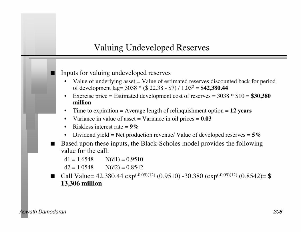
Aswath Damodaran 208
Valuing Undeveloped Reserves
Inputs for valuing undeveloped reserves• Value of underlying asset = Value of estimated reserves discounted back for period
of development lag= 3038 * ($ 22.38 - $7) / 1.052 = $42,380.44• Exercise price = Estimated development cost of reserves = 3038 * $10 = $30,380
million• Time to expiration = Average length of relinquishment option = 12 years• Variance in value of asset = Variance in oil prices = 0.03• Riskless interest rate = 9%• Dividend yield = Net production revenue/ Value of developed reserves = 5%
Based upon these inputs, the Black-Scholes model provides the followingvalue for the call:
d1 = 1.6548 N(d1) = 0.9510d2 = 1.0548 N(d2) = 0.8542
Call Value= 42,380.44 exp(-0.05)(12) (0.9510) -30,380 (exp(-0.09)(12) (0.8542)= $13,306 million

Aswath Damodaran 209
Valuing Gulf Oil
In addition, Gulf Oil had free cashflows to the firm from its oil and gasproduction of $915 million from already developed reserves and thesecashflows are likely to continue for ten years (the remaining lifetime ofdeveloped reserves).
The present value of these developed reserves, discounted at the weightedaverage cost of capital of 12.5%, yields:
• Value of already developed reserves = 915 (1 - 1.125-10)/.125 = $5065.83 Adding the value of the developed and undeveloped reserves
Value of undeveloped reserves = $ 13,306 millionValue of production in place = $ 5,066 millionTotal value of firm = $ 18,372 millionLess Outstanding Debt = $ 9,900 millionValue of Equity = $ 8,472 millionValue per share = $ 8,472/165.3 = $51.25

Aswath Damodaran 210
Example 3: Valuing an Expansion Option
Ambev is considering introducing a soft drink to the U.S. market. The drinkwill initially be introduced only in the metropolitan areas of the U.S. and thecost of this “limited introduction” is $ 500 million.
A financial analysis of the cash flows from this investment suggests that thepresent value of the cash flows from this investment to Ambev will be only $400 million. Thus, by itself, the new investment has a negative NPV of $ 100million.
If the initial introduction works out well, Ambev could go ahead with a full-scale introduction to the entire market with an additional investment of $1 billion any time over the next 5 years. While the current expectation is thatthe cash flows from having this investment is only $ 750 million, there isconsiderable uncertainty about both the potential for the drink, leading tosignificant variance in this estimate.
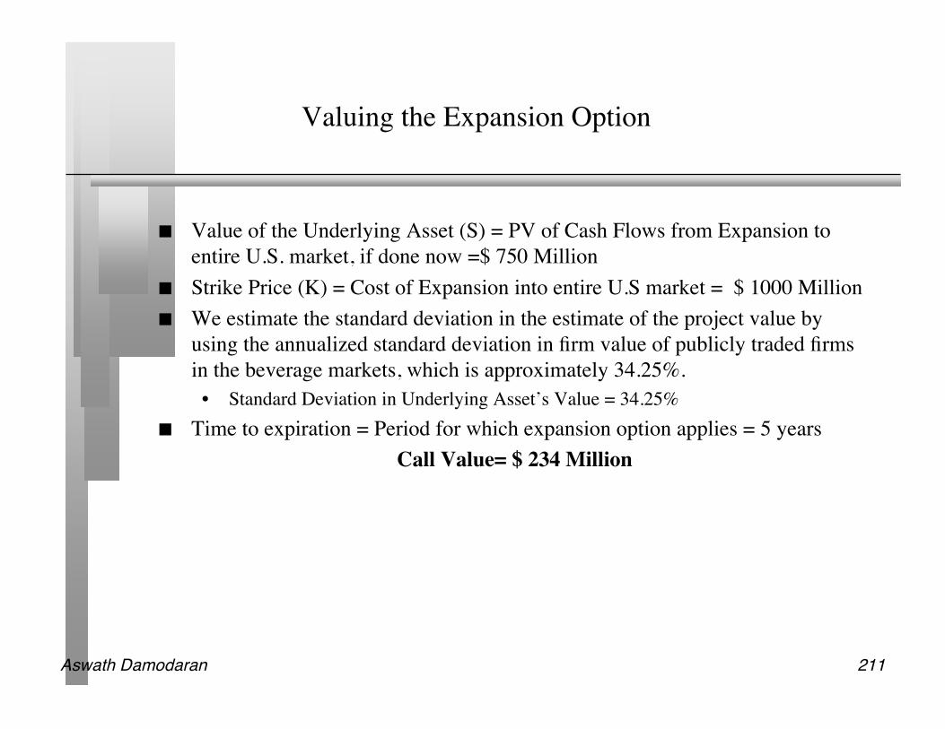
Aswath Damodaran 211
Valuing the Expansion Option
Value of the Underlying Asset (S) = PV of Cash Flows from Expansion toentire U.S. market, if done now =$ 750 Million
Strike Price (K) = Cost of Expansion into entire U.S market = $ 1000 Million We estimate the standard deviation in the estimate of the project value by
using the annualized standard deviation in firm value of publicly traded firmsin the beverage markets, which is approximately 34.25%.
• Standard Deviation in Underlying Asset’s Value = 34.25% Time to expiration = Period for which expansion option applies = 5 years
Call Value= $ 234 Million
Aswath Damodaran 212
Example 4: Valuing Equity in a Deeply Troubled Firm
Assume that you have a firm whose assets are currently valued at $100million and that the standard deviation in this asset value is 40%.
Further, assume that the face value of debt is $80 million (It is zero coupondebt with 10 years left to maturity).
If the ten-year treasury bond rate is 10%,• how much is the equity worth?• What should the interest rate on debt be?

Aswath Damodaran 213
Model Parameters
Value of the underlying asset = S = Value of the firm = $ 100 million Exercise price = K = Face Value of outstanding debt = $ 80 million Life of the option = t = Life of zero-coupon debt = 10 years Variance in the value of the underlying asset = σ2 = Variance in firm value =
0.16 Riskless rate = r = Treasury bond rate corresponding to option life = 10%

Aswath Damodaran 214
Valuing Equity as a Call Option
Based upon these inputs, the Black-Scholes model provides the followingvalue for the call:
• d1 = 1.5994 N(d1) = 0.9451• d2 = 0.3345 N(d2) = 0.6310
Value of the call = 100 (0.9451) - 80 exp(-0.10)(10) (0.6310) = $75.94 million Value of the outstanding debt = $100 - $75.94 = $24.06 million Interest rate on debt = ($ 80 / $24.06)1/10 -1 = 12.77%

Aswath Damodaran 215
The Effect of Catastrophic Drops in Value
Assume now that a catastrophe wipes out half the value of this firm (the valuedrops to $ 50 million), while the face value of the debt remains at $ 80million. What will happen to the equity value of this firm?
It will drop in value to $ 25.94 million [ $ 50 million - market value of debtfrom previous page]
It will be worth nothing since debt outstanding > Firm Value It will be worth more than $ 25.94 million

Aswath Damodaran 216
Valuing Equity in the Troubled Firm
Value of the underlying asset = S = Value of the firm = $ 50 million Exercise price = K = Face Value of outstanding debt = $ 80 million Life of the option = t = Life of zero-coupon debt = 10 years Variance in the value of the underlying asset = σ2 = Variance in firm value =
0.16 Riskless rate = r = Treasury bond rate corresponding to option life = 10%

Aswath Damodaran 217
The Value of Equity as an Option
Based upon these inputs, the Black-Scholes model provides the followingvalue for the call:
• d1 = 1.0515 N(d1) = 0.8534• d2 = -0.2135 N(d2) = 0.4155
Value of the call = 50 (0.8534) - 80 exp(-0.10)(10) (0.4155) = $30.44 million Value of the bond= $50 - $30.44 = $19.56 million The equity in this firm drops by, because of the option characteristics of
equity. This might explain why stock in firms, which are in Chapter 11 and
essentially bankrupt, still has value.

Aswath Damodaran 218
Equity value persists ..
Value of Equity as Firm Value Changes
0
10
20
30
40
50
60
70
80
100 90 80 70 60 50 40 30 20 10
Value of Firm ($ 80 Face Value of Debt)
Valu
e
of
Equit
y

Aswath Damodaran 219
Obtaining option pricing inputs - Some real world problems
The examples that have been used to illustrate the use of option pricing theoryto value equity have made some simplifying assumptions. Among them arethe following:
(1) There were only two claim holders in the firm - debt and equity.(2) There is only one issue of debt outstanding and it can be retired at face value.(3) The debt has a zero coupon and no special features (convertibility, put clauses etc.)(4) The value of the firm and the variance in that value can be estimated.

Aswath Damodaran 220
Real World Approaches to Getting inputs
Input Estimation Process
Value of the Firm • Cumulate market values of equity and debt (or)
• Value the assets in place using FCFF and WACC (or)
• Use cumulated market value of assets, if traded.
Variance in Firm Value • If stocks and bonds are traded,
!2firm = we2 !e2 + wd2 !d2 + 2 we wd "ed !e !d
where !e2 = variance in the stock price
we = MV weight of Equity
!d2 = the variance in the bond price w d = MV weight of debt
• If not traded, use variances of similarly rated bonds.
• Use average firm value variance from the industry in which
company operates.
Value of the Debt • If the debt is short term, you can use only the face or book value
of the debt.
• If the debt is long term and coupon bearing, add the cumulated
nominal value of these coupons to the face value of the debt.
Maturity of the Debt • Face value weighted duration of bonds outstanding (or)
• If not available, use weighted maturity
Aswath Damodaran 221
Valuing Equity as an option - Eurotunnel in early 1998
Eurotunnel has been a financial disaster since its opening• In 1997, Eurotunnel had earnings before interest and taxes of -£56 million and net
income of -£685 million• At the end of 1997, its book value of equity was -£117 million
It had £8,865 million in face value of debt outstanding• The weighted average duration of this debt was 10.93 years Debt Type Face Value Duration Short term 935 0.50
10 year 2435 6.720 year 3555 12.6Longer 1940 18.2
Total £8,865 mil 10.93 years

Aswath Damodaran 222
The Basic DCF Valuation
The value of the firm estimated using projected cashflows to the firm,discounted at the weighted average cost of capital was £2,312 million.
This was based upon the following assumptions –• Revenues will grow 5% a year in perpetuity.• The COGS which is currently 85% of revenues will drop to 65% of revenues in yr
5 and stay at that level.• Capital spending and depreciation will grow 5% a year in perpetuity.• There are no working capital requirements.• The debt ratio, which is currently 95.35%, will drop to 70% after year 5. The cost
of debt is 10% in high growth period and 8% after that.• The beta for the stock will be 1.10 for the next five years, and drop to 0.8 after the
next 5 years.• The long term bond rate is 6%.

Aswath Damodaran 223
Other Inputs
The stock has been traded on the London Exchange, and the annualized stddeviation based upon ln (prices) is 41%.
There are Eurotunnel bonds, that have been traded; the annualized stddeviation in ln(price) for the bonds is 17%.
• The correlation between stock price and bond price changes has been 0.5. Theproportion of debt in the capital structure during the period (1992-1996) was 85%.
• Annualized variance in firm value= (0.15)2 (0.41)2 + (0.85)2 (0.17)2 + 2 (0.15) (0.85)(0.5)(0.41)(0.17)= 0.0335
The 15-year bond rate is 6%. (I used a bond with a duration of roughly 11years to match the life of my option)

Aswath Damodaran 224
Valuing Eurotunnel Equity and Debt
Inputs to Model• Value of the underlying asset = S = Value of the firm = £2,312 million• Exercise price = K = Face Value of outstanding debt = £8,865 million• Life of the option = t = Weighted average duration of debt = 10.93 years• Variance in the value of the underlying asset = σ2 = Variance in firm value =
0.0335• Riskless rate = r = Treasury bond rate corresponding to option life = 6%
Based upon these inputs, the Black-Scholes model provides the followingvalue for the call:
d1 = -0.8337 N(d1) = 0.2023d2 = -1.4392 N(d2) = 0.0751
Value of the call = 2312 (0.2023) - 8,865 exp(-0.06)(10.93) (0.0751) = £122million
Appropriate interest rate on debt = (8865/2190)(1/10.93)-1= 13.65%
Aswath Damodaran 225
Key Tests for Real Options
Is there an option embedded in this asset/ decision?• Can you identify the underlying asset?• Can you specify the contigency under which you will get payoff?
Is there exclusivity?• If yes, there is option value.• If no, there is none.• If in between, you have to scale value.
Can you use an option pricing model to value the real option?• Is the underlying asset traded?• Can the option be bought and sold?• Is the cost of exercising the option known and clear?
Aswath Damodaran 226
In Closing…
There are real options everywhere. Most of them have no significant economic value because there is no
exclusivity associated with using them. When options have significant economic value, the inputs needed to value
them in a binomial model can be used in more traditional approaches(decision trees) to yield equivalent value.
The real value from real options lies in• Recognizing that building in flexibility and escape hatches into large decisions has
value• Insights we get on understanding how and why companies behave the way they do
in investment analysis and capital structure choices.

Aswath Damodaran 227
Back to Lemmings...