Valuation Multiples: A Primer Global Equity Research · Valuation Primer Series Issue 1 This is the...
47
Global Global Equity Research Peter Suozzo +852-2971 6121 [email protected] Stephen Cooper +44-20-7568 1962 [email protected] Gillian Sutherland +44-20-7568 8369 [email protected] Zhen Deng +1-212-713 9921 [email protected] Valuation Primer Series Issue 1 ■ This is the first in a series of primers on fundamental valuation topics such as discounted cash flow, valuation multiples and cost of capital. ■ This document explains how to calculate and use multiples commonly used in equity analysis. ■ We discuss the differences between equity and enterprise multiples, show how target or ‘fair’ multiples can be derived from underlying value drivers and discuss the ways multiples can be used in valuation. For each multiple, we show its derivation, discuss its strengths and weaknesses, and suggest appropriate use. Valuation & Accounting November 2001 www.ubswarburg.com/researchweb In addition to the UBS Warburg web site our research products are available over third-party systems provided or serviced by: Bloomberg, First Call, I/B/E/S, IFIS, Multex, QUICK and Reuters UBS Warburg is a business group of UBS AG Valuation Multiples: A Primer
Transcript of Valuation Multiples: A Primer Global Equity Research · Valuation Primer Series Issue 1 This is the...

Global
GlobalEquity
Research
Peter Suozzo+852-2971 6121
Stephen Cooper+44-20-7568 1962
Gillian Sutherland+44-20-7568 8369
Zhen Deng+1-212-713 [email protected]
Valuation Primer Series Issue 1
■■■■ This is the first in a series of primers on fundamental valuation topics such asdiscounted cash flow, valuation multiples and cost of capital.
■■■■ This document explains how to calculate and use multiples commonly used inequity analysis.
■■■■ We discuss the differences between equity and enterprise multiples, show howtarget or ‘fair’ multiples can be derived from underlying value drivers anddiscuss the ways multiples can be used in valuation. For each multiple, we showits derivation, discuss its strengths and weaknesses, and suggest appropriate use.
Valuation & Accounting November 2001
www.ubswarburg.com/researchweb
In addition to theUBS Warburg web site
our research products are availableover third-party systemsprovided or serviced by:
Bloomberg, First Call, I/B/E/S, IFIS,Multex, QUICK and Reuters
UBS Warburg is a businessgroup of UBS AG
Valuation Multiples: A Primer
Valuation Multiples: A Primer November 2001
2 UBS Warburg
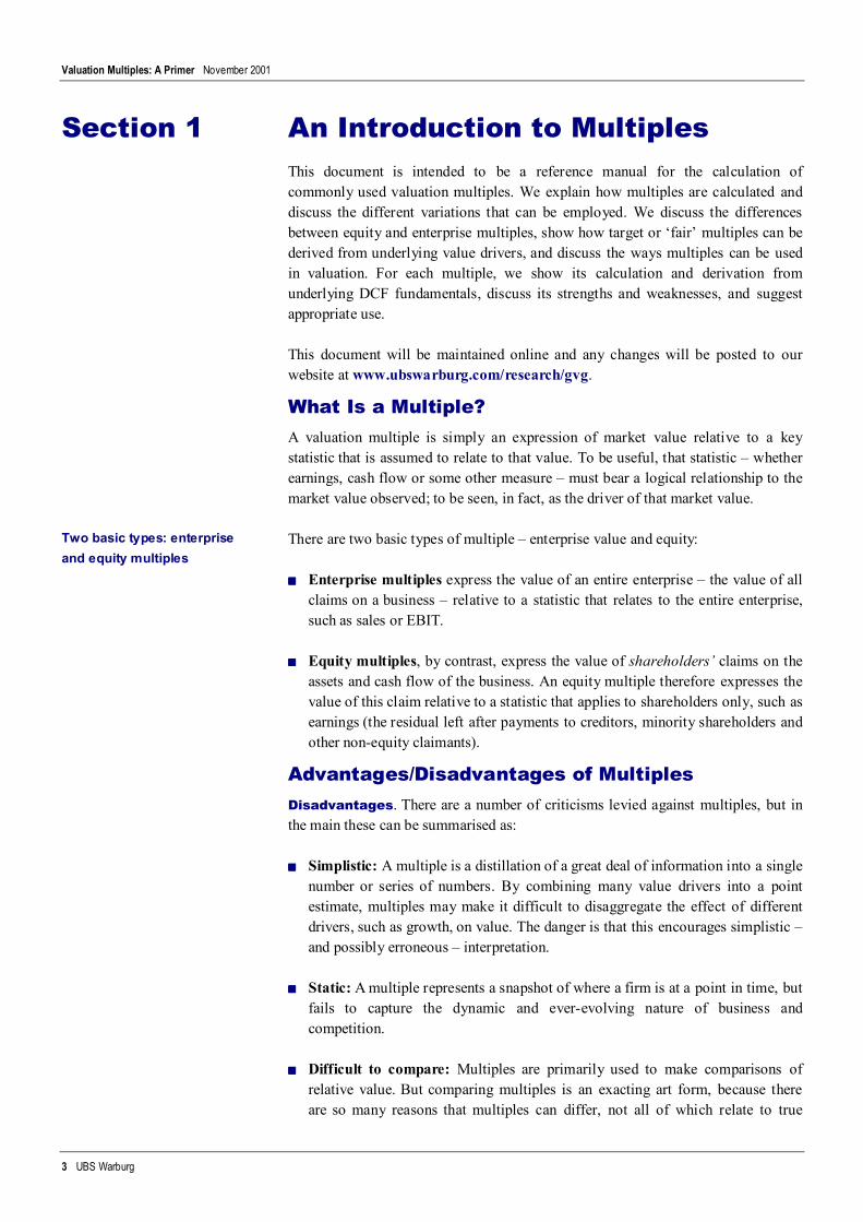
Contents page
An Introduction to Multiples ........................................................................... 3
— What Is a Multiple? ......................................................................... 3
— Advantages/Disadvantages of Multiples ........................................... 3
— Enterprise versus Equity Multiples ................................................... 5
— Why Multiples Vary......................................................................... 5
— Choosing the Pricing Date............................................................. 10
Target Valuation Multiples ........................................................................... 13
— What Is a Target Multiple?............................................................. 13
— Single-stage Target Multiples ........................................................ 14
— Two-stage Target Multiples ........................................................... 15
— Examples..................................................................................... 16
— Assumptions Used in Target Multiple Formulas .............................. 17
— The Effect of Growth on Value....................................................... 18
Using Valuation Multiples ............................................................................ 20
Enterprise Value Multiples........................................................................... 24
— What Is Enterprise Value?............................................................. 24
— Why Use Enterprise Value Multiples? ............................................ 25
— Potential Problems in Calculating EV ............................................. 26
— Enterprise Value Multiples............................................................. 28
Equity Multiples .......................................................................................... 37
— What Are Equity Multiples? ........................................................... 37
— Equity Multiples ............................................................................ 37
Appendix: Derivation of Target Multiple Formulas ......................................... 42
Peter Suozzo+852-2971 6121
Stephen Cooper+44-20-7568 1962
Gillian Sutherland+44-20-7568 8369
Zhen Deng+1-212-713 [email protected]
For research, valuation models and more on equity analysis go to the Global Valuation Group website...www.ubswarburg.com/research/gvg
Valuation Multiples: A Primer November 2001
3 UBS Warburg
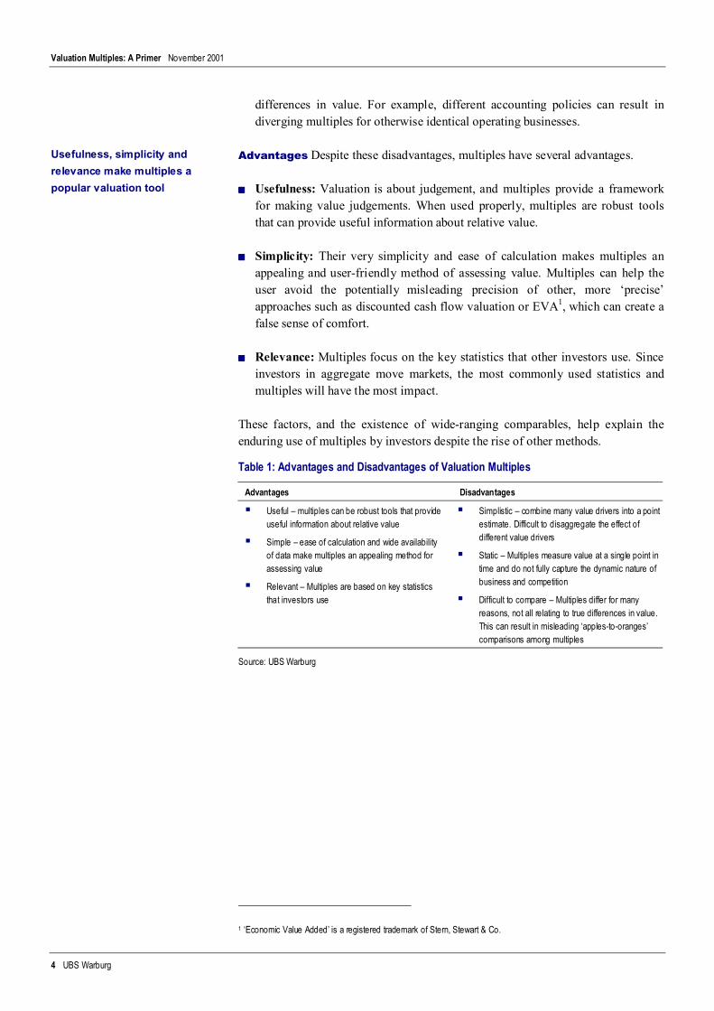
An Introduction to MultiplesThis document is intended to be a reference manual for the calculation ofcommonly used valuation multiples. We explain how multiples are calculated anddiscuss the different variations that can be employed. We discuss the differencesbetween equity and enterprise multiples, show how target or ‘fair’ multiples can bederived from underlying value drivers, and discuss the ways multiples can be usedin valuation. For each multiple, we show its calculation and derivation fromunderlying DCF fundamentals, discuss its strengths and weaknesses, and suggestappropriate use.
This document will be maintained online and any changes will be posted to ourwebsite at www.ubswarburg.com/research/gvg.
What Is a Multiple?A valuation multiple is simply an expression of market value relative to a keystatistic that is assumed to relate to that value. To be useful, that statistic – whetherearnings, cash flow or some other measure – must bear a logical relationship to themarket value observed; to be seen, in fact, as the driver of that market value.
There are two basic types of multiple – enterprise value and equity:
■■■■ Enterprise multiples express the value of an entire enterprise – the value of allclaims on a business – relative to a statistic that relates to the entire enterprise,such as sales or EBIT.
■■■■ Equity multiples, by contrast, express the value of shareholders’ claims on theassets and cash flow of the business. An equity multiple therefore expresses thevalue of this claim relative to a statistic that applies to shareholders only, such asearnings (the residual left after payments to creditors, minority shareholders andother non-equity claimants).
Advantages/Disadvantages of MultiplesDisadvantages. There are a number of criticisms levied against multiples, but inthe main these can be summarised as:
■■■■ Simplistic: A multiple is a distillation of a great deal of information into a singlenumber or series of numbers. By combining many value drivers into a pointestimate, multiples may make it difficult to disaggregate the effect of differentdrivers, such as growth, on value. The danger is that this encourages simplistic –and possibly erroneous – interpretation.
■■■■ Static: A multiple represents a snapshot of where a firm is at a point in time, butfails to capture the dynamic and ever-evolving nature of business andcompetition.
■■■■ Difficult to compare: Multiples are primarily used to make comparisons ofrelative value. But comparing multiples is an exacting art form, because thereare so many reasons that multiples can differ, not all of which relate to true
Section 1
Two basic types: enterpriseand equity multiples
Valuation Multiples: A Primer November 2001
4 UBS Warburg
differences in value. For example, different accounting policies can result indiverging multiples for otherwise identical operating businesses.
Advantages Despite these disadvantages, multiples have several advantages.
■■■■ Usefulness: Valuation is about judgement, and multiples provide a frameworkfor making value judgements. When used properly, multiples are robust toolsthat can provide useful information about relative value.
■■■■ Simplicity: Their very simplicity and ease of calculation makes multiples anappealing and user-friendly method of assessing value. Multiples can help theuser avoid the potentially misleading precision of other, more ‘precise’approaches such as discounted cash flow valuation or EVA1, which can create afalse sense of comfort.
■■■■ Relevance: Multiples focus on the key statistics that other investors use. Sinceinvestors in aggregate move markets, the most commonly used statistics andmultiples will have the most impact.
These factors, and the existence of wide-ranging comparables, help explain theenduring use of multiples by investors despite the rise of other methods.
Table 1: Advantages and Disadvantages of Valuation Multiples
Advantages Disadvantages
Useful – multiples can be robust tools that provideuseful information about relative value
Simple – ease of calculation and wide availabilityof data make multiples an appealing method forassessing value
Relevant – Multiples are based on key statisticsthat investors use
Simplistic – combine many value drivers into a pointestimate. Difficult to disaggregate the effect ofdifferent value drivers
Static – Multiples measure value at a single point intime and do not fully capture the dynamic nature ofbusiness and competition
Difficult to compare – Multiples differ for manyreasons, not all relating to true differences in value.This can result in misleading ‘apples-to-oranges’comparisons among multiples
Source: UBS Warburg
1 ‘Economic Value Added’ is a registered trademark of Stern, Stewart & Co.
Usefulness, simplicity andrelevance make multiples apopular valuation tool
Valuation Multiples: A Primer November 2001
5 UBS Warburg
Enterprise versus Equity MultiplesIn the table below we have summarised the relative advantages of using enterprisevalue (EV) versus equity multiples and vice versa. For more details please see page25 below.
Table 2: Enterprise Value versus Equity Multiples
Enterprise value multiples Equity multiples
Allow the user to focus on statistics whereaccounting policy differences can be minimised(EBITDA, OpFCF)
Avoid the influence of capital structure on equityvalue multiples
More comprehensive (apply to the entire enterprise)
Wider range of multiples possible
Easier to apply to cash flow
Enables the user to exclude non-core assets
More relevant to equity valuation
More reliable (estimating enterprise valueinvolves more subjectivity, especially in thevaluation of non-core assets)
More familiar to investors
Source: UBS Warburg
Why Multiples VaryThere are four primary reasons why multiples can vary:
■■■■ Differences in the quality of the business (ie differences in value drivers)
■■■■ Accounting differences
■■■■ Fluctuations in cash flow or profit (ie they are unrepresentative of the future)
■■■■ Mispricing
1. Differences in the Quality of the BusinessAll things equal, higher-quality businesses deserve higher valuation multiples. Thisis another way of saying that there are qualitative differences in the fundamentalunderlying drivers of valuation, such as quality of management, availableinvestment opportunities, strategy and branding. These can be distilled down to fourquantitative valuation drivers: return on capital, cost of capital, growth and durationof growth.
As investors, we are interested in how to allow for differences in these valuedrivers. How much is growth worth? What is the impact of a change in return oncapital? We consider these issues in Target Valuation Multiples, starting on page13.
2. Accounting DifferencesDifferences in accounting policies that do not affect cash flow do not affect value.But accounting policy differences do affect profit multiples and, as a result,differences in multiples can paint a misleading picture of relative valuation.
For example, consider two identical companies with 20 of goodwill on the balancesheet and 10 in pre-goodwill profit. Company A does not amortise goodwill whileCompany B amortises over 10 years (amortisation of 2 per year).
Differences in accountingpolicies that do not affectcash flow do not affectvalue
Valuation Multiples: A Primer November 2001
6 UBS Warburg
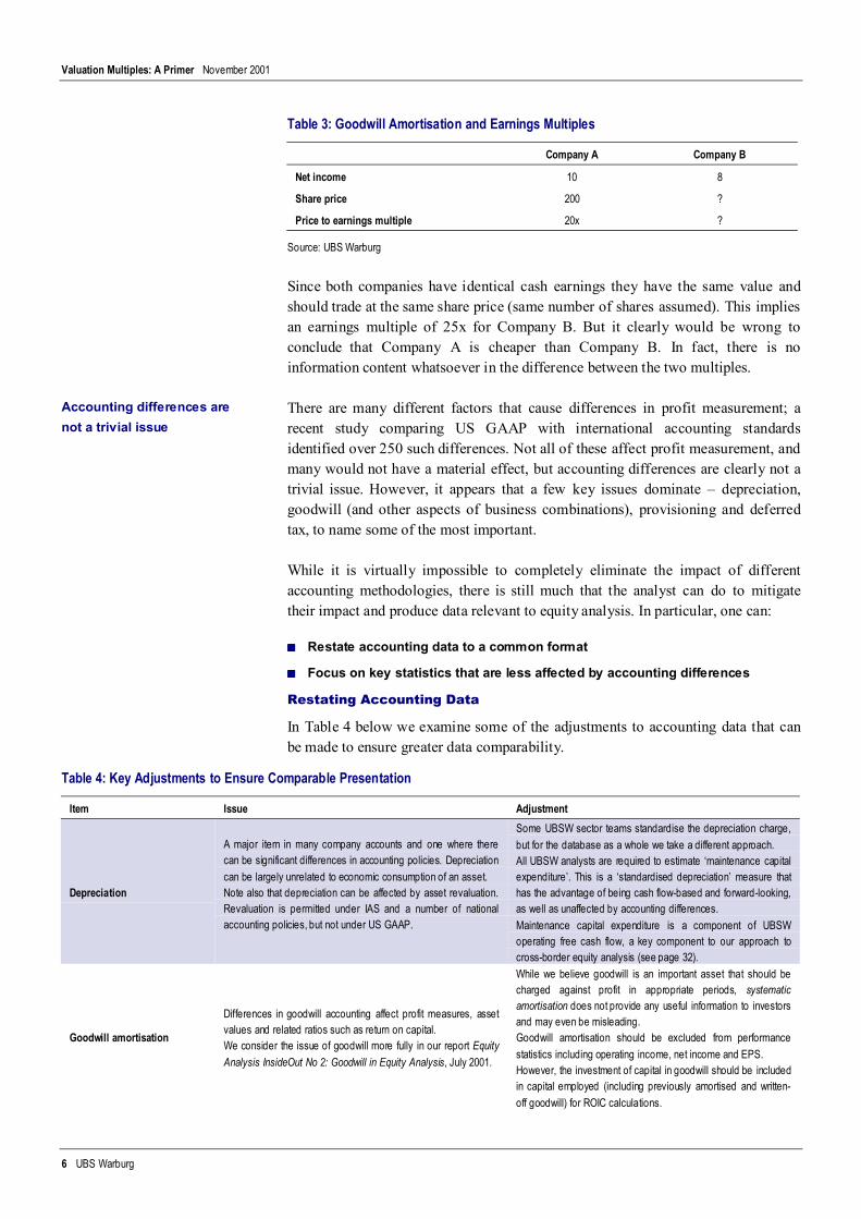
Table 3: Goodwill Amortisation and Earnings Multiples
Company A Company B
Net income 10 8
Share price 200 ?
Price to earnings multiple 20x ?
Source: UBS Warburg
Since both companies have identical cash earnings they have the same value andshould trade at the same share price (same number of shares assumed). This impliesan earnings multiple of 25x for Company B. But it clearly would be wrong toconclude that Company A is cheaper than Company B. In fact, there is noinformation content whatsoever in the difference between the two multiples.
There are many different factors that cause differences in profit measurement; arecent study comparing US GAAP with international accounting standardsidentified over 250 such differences. Not all of these affect profit measurement, andmany would not have a material effect, but accounting differences are clearly not atrivial issue. However, it appears that a few key issues dominate – depreciation,goodwill (and other aspects of business combinations), provisioning and deferredtax, to name some of the most important.
While it is virtually impossible to completely eliminate the impact of differentaccounting methodologies, there is still much that the analyst can do to mitigatetheir impact and produce data relevant to equity analysis. In particular, one can:
■■■■ Restate accounting data to a common format
■■■■ Focus on key statistics that are less affected by accounting differences
Restating Accounting Data
In Table 4 below we examine some of the adjustments to accounting data that canbe made to ensure greater data comparability.
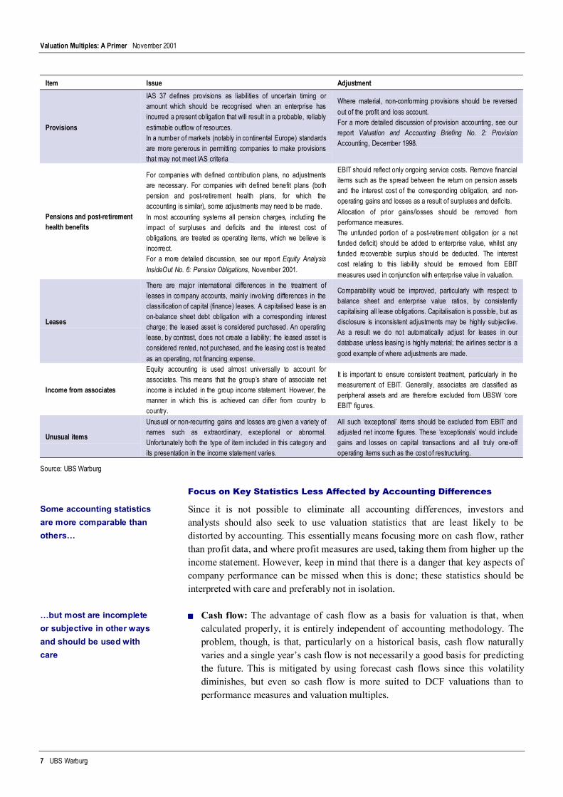
Table 4: Key Adjustments to Ensure Comparable Presentation
Item Issue Adjustment
Depreciation
A major item in many company accounts and one where therecan be significant differences in accounting policies. Depreciationcan be largely unrelated to economic consumption of an asset.Note also that depreciation can be affected by asset revaluation.Revaluation is permitted under IAS and a number of nationalaccounting policies, but not under US GAAP.
Some UBSW sector teams standardise the depreciation charge,but for the database as a whole we take a different approach.All UBSW analysts are required to estimate ‘maintenance capitalexpenditure’. This is a ‘standardised depreciation’ measure thathas the advantage of being cash flow-based and forward-looking,as well as unaffected by accounting differences.Maintenance capital expenditure is a component of UBSWoperating free cash flow, a key component to our approach tocross-border equity analysis (see page 32).
Goodwill amortisation
Differences in goodwill accounting affect profit measures, assetvalues and related ratios such as return on capital.We consider the issue of goodwill more fully in our report EquityAnalysis InsideOut No 2: Goodwill in Equity Analysis, July 2001.
While we believe goodwill is an important asset that should becharged against profit in appropriate periods, systematicamortisation does not provide any useful information to investorsand may even be misleading.Goodwill amortisation should be excluded from performancestatistics including operating income, net income and EPS.However, the investment of capital in goodwill should be includedin capital employed (including previously amortised and written-off goodwill) for ROIC calculations.
Accounting differences arenot a trivial issue
Valuation Multiples: A Primer November 2001
7 UBS Warburg
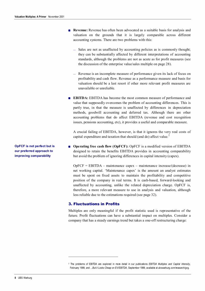
Item Issue Adjustment
Provisions
IAS 37 defines provisions as liabilities of uncertain timing oramount which should be recognised when an enterprise hasincurred a present obligation that will result in a probable, reliablyestimable outflow of resources.In a number of markets (notably in continental Europe) standardsare more generous in permitting companies to make provisionsthat may not meet IAS criteria
Where material, non-conforming provisions should be reversedout of the profit and loss account.For a more detailed discussion of provision accounting, see ourreport Valuation and Accounting Briefing No. 2: ProvisionAccounting, December 1998.
Pensions and post-retirementhealth benefits
For companies with defined contribution plans, no adjustmentsare necessary. For companies with defined benefit plans (bothpension and post-retirement health plans, for which theaccounting is similar), some adjustments may need to be made.In most accounting systems all pension charges, including theimpact of surpluses and deficits and the interest cost ofobligations, are treated as operating items, which we believe isincorrect.For a more detailed discussion, see our report Equity AnalysisInsideOut No. 6: Pension Obligations, November 2001.
EBIT should reflect only ongoing service costs. Remove financialitems such as the spread between the return on pension assetsand the interest cost of the corresponding obligation, and non-operating gains and losses as a result of surpluses and deficits.Allocation of prior gains/losses should be removed fromperformance measures.The unfunded portion of a post-retirement obligation (or a netfunded deficit) should be added to enterprise value, whilst anyfunded recoverable surplus should be deducted. The interestcost relating to this liability should be removed from EBITmeasures used in conjunction with enterprise value in valuation.
Leases
There are major international differences in the treatment ofleases in company accounts, mainly involving differences in theclassification of capital (finance) leases. A capitalised lease is anon-balance sheet debt obligation with a corresponding interestcharge; the leased asset is considered purchased. An operatinglease, by contrast, does not create a liability; the leased asset isconsidered rented, not purchased, and the leasing cost is treatedas an operating, not financing expense.
Comparability would be improved, particularly with respect tobalance sheet and enterprise value ratios, by consistentlycapitalising all lease obligations. Capitalisation is possible, but asdisclosure is inconsistent adjustments may be highly subjective.As a result we do not automatically adjust for leases in ourdatabase unless leasing is highly material; the airlines sector is agood example of where adjustments are made.
Income from associates
Equity accounting is used almost universally to account forassociates. This means that the group’s share of associate netincome is included in the group income statement. However, themanner in which this is achieved can differ from country tocountry.
It is important to ensure consistent treatment, particularly in themeasurement of EBIT. Generally, associates are classified asperipheral assets and are therefore excluded from UBSW ‘coreEBIT’ figures.
Unusual items
Unusual or non-recurring gains and losses are given a variety ofnames such as extraordinary, exceptional or abnormal.Unfortunately both the type of item included in this category andits presentation in the income statement varies.
All such ‘exceptional’ items should be excluded from EBIT andadjusted net income figures. These ‘exceptionals’ would includegains and losses on capital transactions and all truly one-offoperating items such as the cost of restructuring.
Source: UBS Warburg
Focus on Key Statistics Less Affected by Accounting Differences
Since it is not possible to eliminate all accounting differences, investors andanalysts should also seek to use valuation statistics that are least likely to bedistorted by accounting. This essentially means focusing more on cash flow, ratherthan profit data, and where profit measures are used, taking them from higher up theincome statement. However, keep in mind that there is a danger that key aspects ofcompany performance can be missed when this is done; these statistics should beinterpreted with care and preferably not in isolation.
■■■■ Cash flow: The advantage of cash flow as a basis for valuation is that, whencalculated properly, it is entirely independent of accounting methodology. Theproblem, though, is that, particularly on a historical basis, cash flow naturallyvaries and a single year’s cash flow is not necessarily a good basis for predictingthe future. This is mitigated by using forecast cash flows since this volatilitydiminishes, but even so cash flow is more suited to DCF valuations than toperformance measures and valuation multiples.
Some accounting statisticsare more comparable thanothers…
…but most are incompleteor subjective in other waysand should be used withcare
Valuation Multiples: A Primer November 2001
8 UBS Warburg
■■■■ Revenue: Revenue has often been advocated as a suitable basis for analysis andvaluation on the grounds that it is largely comparable across differentaccounting systems. There are two problems with this:
— Sales are not as unaffected by accounting policies as is commonly thought;they can be substantially affected by different interpretations of accountingstandards, although the problems are not as acute as for profit measures (seethe discussion of the enterprise value/sales multiple on page 28).
— Revenue is an incomplete measure of performance given its lack of focus onprofitability and cash flow. Revenue as a performance measure and basis forvaluation should be a last resort if other more relevant profit measures areunavailable or unreliable.
■■■■ EBITDA: EBITDA has become the most common measure of performance andvalue that supposedly overcomes the problem of accounting differences. This ispartly true, in that the measure is unaffected by differences in depreciationmethods, goodwill accounting and deferred tax. Although there are otheraccounting problems that do affect EBITDA (revenue and cost recognitionissues, pensions accounting, etc), it provides a useful and comparable measure.
A crucial failing of EBITDA, however, is that it ignores the very real costs ofcapital expenditure and taxation that should (and do) affect value.2
■■■■ Operating free cash flow (OpFCF): OpFCF is a modified version of EBITDAdesigned to retain the benefits EBITDA provides in accounting comparabilitybut avoid the problem of ignoring differences in capital intensity (capex).
OpFCF = EBITDA – maintenance capex – maintenance increase/(decrease) innet working capital. ‘Maintenance capex’ is the amount an analyst estimatesmust be spent on fixed assets to maintain the profitability and competitiveposition of the company in real terms. It is cash-based, forward-looking andunaffected by accounting, unlike the related depreciation charge. OpFCF is,therefore, a more relevant measure to use in analysis and valuation, althoughless reliable due to the estimations required (see page 32).
3. Fluctuations in ProfitsMultiples are only meaningful if the profit statistic used is representative of thefuture. Profit fluctuations can have a substantial impact on multiples. Consider acompany that has a steady earnings trend but takes a one-off restructuring charge:
2 The problems of EBITDA are explored in more detail in our publications EBITDA Multiples and Capital Intensity,February 1999, and ...But it Looks Cheap on EV/EBITDA, September 1999, available at ubswarburg.com/research/gvg.
OpFCF is not perfect but isour preferred approach toimproving comparability
Valuation Multiples: A Primer November 2001
9 UBS Warburg
Table 5: Fluctuating Earnings and the PE Multiple
1999 2000 2001 2002E 2003E
Earnings 10 12 14 3 17
Average price 200 220 260 ? ?
Historical priced PE multiple 20.0x 18.3x 18.6x ? ?
Source: UBS Warburg
Since earnings will recover in 2003, it is unlikely that the price will collapse in2002 simply because of a temporary drop in earnings; investors will ‘look through’2002 earnings and the earnings multiple for 2002 is therefore likely to be very high.A naive comparison of this multiple with that of peers or the sector will not beilluminating and is unlikely in itself to provide an opportunity to identifymispricing.
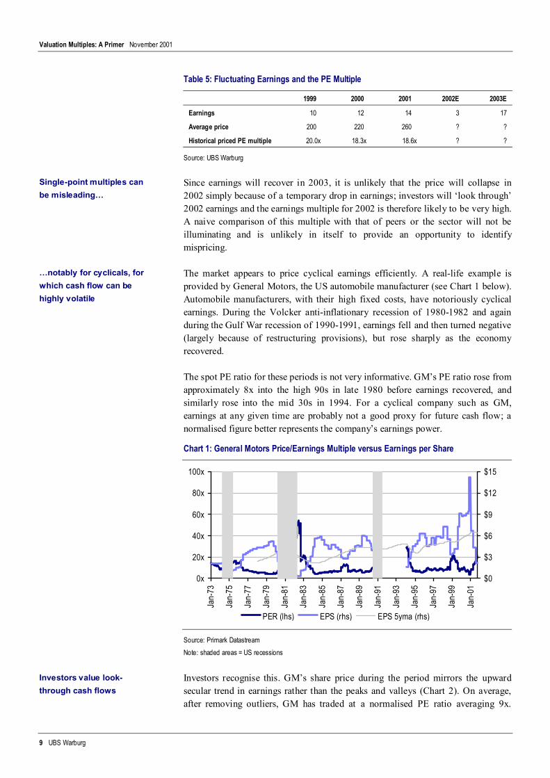
The market appears to price cyclical earnings efficiently. A real-life example isprovided by General Motors, the US automobile manufacturer (see Chart 1 below).Automobile manufacturers, with their high fixed costs, have notoriously cyclicalearnings. During the Volcker anti-inflationary recession of 1980-1982 and againduring the Gulf War recession of 1990-1991, earnings fell and then turned negative(largely because of restructuring provisions), but rose sharply as the economyrecovered.
The spot PE ratio for these periods is not very informative. GM’s PE ratio rose fromapproximately 8x into the high 90s in late 1980 before earnings recovered, andsimilarly rose into the mid 30s in 1994. For a cyclical company such as GM,earnings at any given time are probably not a good proxy for future cash flow; anormalised figure better represents the company’s earnings power.
Chart 1: General Motors Price/Earnings Multiple versus Earnings per Share
0x
20x
40x
60x
80x
100x
Jan-
73
Jan-
75
Jan-
77
Jan-
79
Jan-
81
Jan-
83
Jan-
85
Jan-
87
Jan-
89
Jan-
91
Jan-
93
Jan-
95
Jan-
97
Jan-
99
Jan-
01
$0
$3
$6
$9
$12
$15
PER (lhs) EPS (rhs) EPS 5yma (rhs)
Source: Primark DatastreamNote: shaded areas = US recessions
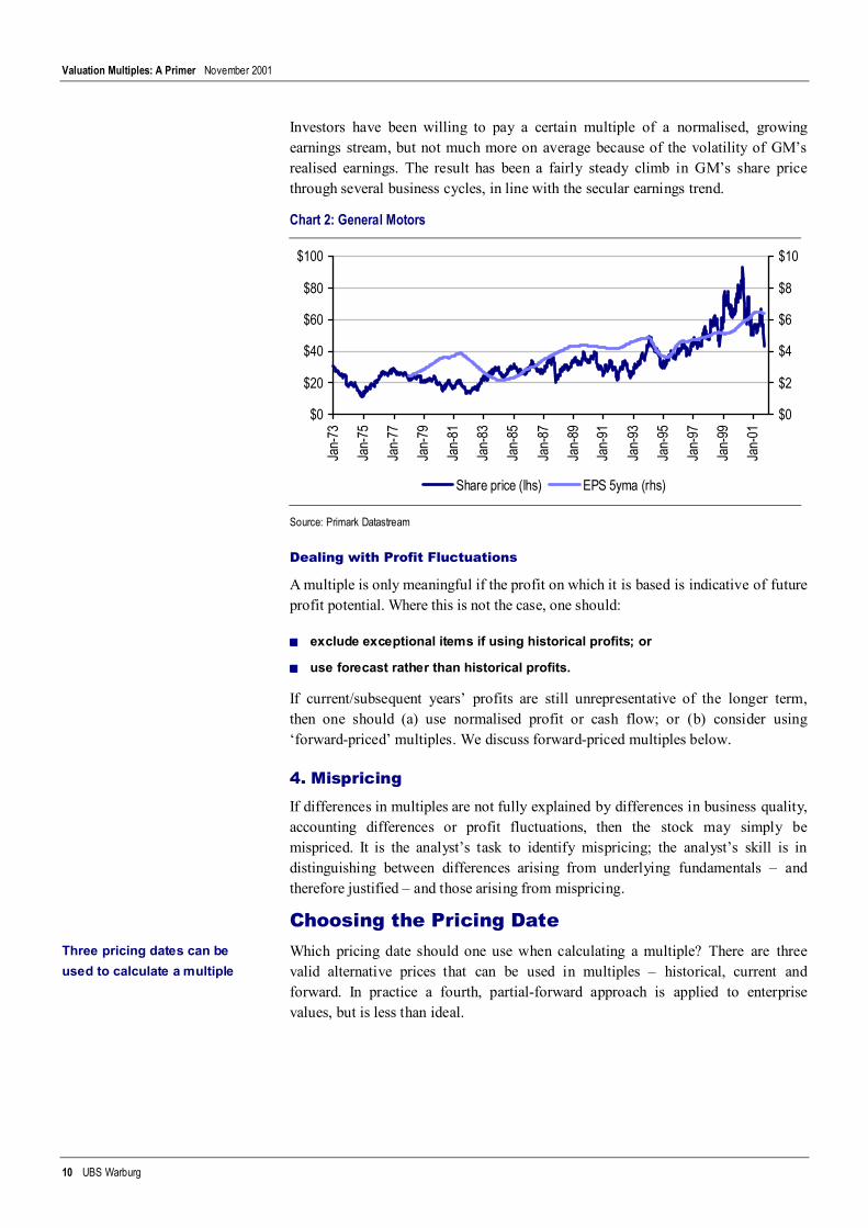
Investors recognise this. GM’s share price during the period mirrors the upwardsecular trend in earnings rather than the peaks and valleys (Chart 2). On average,after removing outliers, GM has traded at a normalised PE ratio averaging 9x.
Single-point multiples canbe misleading…
…notably for cyclicals, forwhich cash flow can behighly volatile
Investors value look-through cash flows
Valuation Multiples: A Primer November 2001
10 UBS Warburg
Investors have been willing to pay a certain multiple of a normalised, growingearnings stream, but not much more on average because of the volatility of GM’srealised earnings. The result has been a fairly steady climb in GM’s share pricethrough several business cycles, in line with the secular earnings trend.
Chart 2: General Motors
$0
$20
$40
$60
$80
$100
Jan-
73
Jan-
75
Jan-
77
Jan-
79
Jan-
81
Jan-
83
Jan-
85
Jan-
87
Jan-
89
Jan-
91
Jan-
93
Jan-
95
Jan-
97
Jan-
99
Jan-
01
$0
$2
$4
$6
$8
$10
Share price (lhs) EPS 5yma (rhs)
Source: Primark Datastream
Dealing with Profit Fluctuations
A multiple is only meaningful if the profit on which it is based is indicative of futureprofit potential. Where this is not the case, one should:
■■■■ exclude exceptional items if using historical profits; or
■■■■ use forecast rather than historical profits.
If current/subsequent years’ profits are still unrepresentative of the longer term,then one should (a) use normalised profit or cash flow; or (b) consider using‘forward-priced’ multiples. We discuss forward-priced multiples below.
4. MispricingIf differences in multiples are not fully explained by differences in business quality,accounting differences or profit fluctuations, then the stock may simply bemispriced. It is the analyst’s task to identify mispricing; the analyst’s skill is indistinguishing between differences arising from underlying fundamentals – andtherefore justified – and those arising from mispricing.
Choosing the Pricing DateWhich pricing date should one use when calculating a multiple? There are threevalid alternative prices that can be used in multiples – historical, current andforward. In practice a fourth, partial-forward approach is applied to enterprisevalues, but is less than ideal.
Three pricing dates can beused to calculate a multiple
Valuation Multiples: A Primer November 2001
11 UBS Warburg
Table 6: Alternative Pricing Bases for Multiples
Pricing basis Calculation Profit or cash flow used Use in valuation
Historical Average price or enterprisevalue for a period
Historical profit for thesame period
Establishes a historical tradingrange
Current Current price or enterprisevalue
Any historical or forecastprofit
Investigation of current value – bestto use current year forecast profit
Forward Forward price or enterprisevalue
Forecast profit for aperiod related to theforward price date
Investigation of current value –superior to current-priced multiplefor forecasts beyond one year
Partial-forward
Current market cap plusforecast net debt (appliesto enterprise value only)
Forecast profit for aperiod related to theforward price date
Investigation of current value but thepartial-forward price is inconsistentand difficult to interpret
Source: UBS Warburg
■■■■ Historical-priced multiples: Comparison of historical price or enterprise valuewith historical profits (cash flow, etc). ‘Historical’ price is generally the averagefor year. Historical-priced multiples are used to establish a trading range.
■■■■ Current-priced multiples: Comparison of current price or enterprise value withhistorical or forecast profits – generally one year of historical and two years offorecast profits. Current-priced multiples are used to investigate current value.Current-priced multiples based upon current-year earnings can be comparedwith historical- and forward-priced multiples.
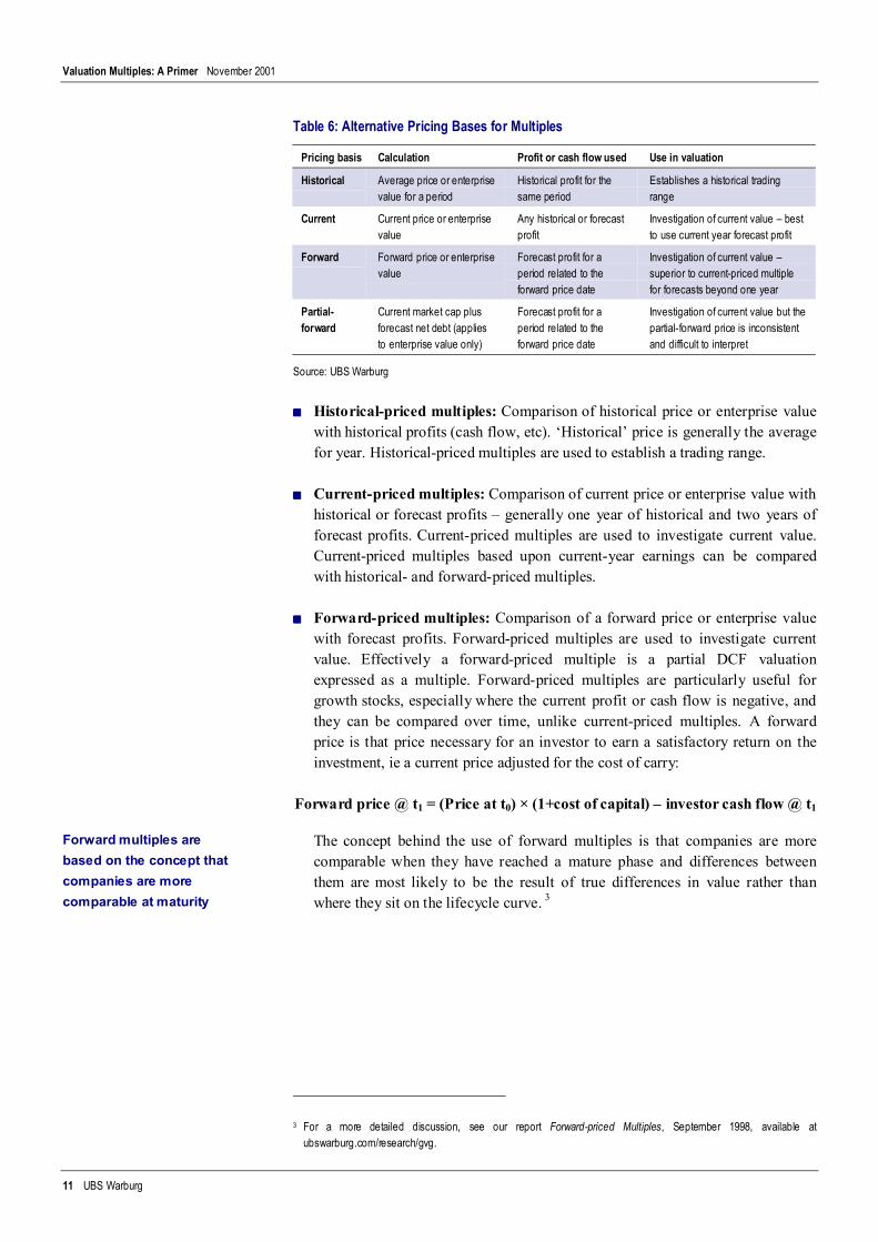
■■■■ Forward-priced multiples: Comparison of a forward price or enterprise valuewith forecast profits. Forward-priced multiples are used to investigate currentvalue. Effectively a forward-priced multiple is a partial DCF valuationexpressed as a multiple. Forward-priced multiples are particularly useful forgrowth stocks, especially where the current profit or cash flow is negative, andthey can be compared over time, unlike current-priced multiples. A forwardprice is that price necessary for an investor to earn a satisfactory return on theinvestment, ie a current price adjusted for the cost of carry:
Forward price @ t1 = (Price at t0) × (1+cost of capital) – investor cash flow @ t1
The concept behind the use of forward multiples is that companies are morecomparable when they have reached a mature phase and differences betweenthem are most likely to be the result of true differences in value rather thanwhere they sit on the lifecycle curve. 3
3 For a more detailed discussion, see our report Forward-priced Multiples, September 1998, available atubswarburg.com/research/gvg.
Forward multiples arebased on the concept thatcompanies are morecomparable at maturity
Valuation Multiples: A Primer November 2001
12 UBS Warburg
Chart 3: Multiple Comparisons and Lifecycles
Time
Growth rate
Multiples likely to be most comparable where
companies are at similar points in their lifecycles
Now Forward
Source: UBS Warburg
■■■■ Partial-forward multiples: In a partial-forward approach, a current equityvalue is combined with a forecast net debt figure in calculating enterprise valueto be compared with forecast profit and cash flow measures. Other componentsof enterprise value, such as minorities and pension provisions, may be includedat either forecast or current value. While this approach does not have theconsistency of the pure forward-priced method above, it does take account of atleast part of the future cash flow that affects value. For example, a company thatis forecast to have lower cash flow than another in the coming years would havea higher net debt and therefore a higher partial-forward EV. Poor cash flow iseffectively penalised by a higher multiple.
Note: Standard enterprise value multiples that appear in UBS Warburgresearch reports are historically priced for historical periods and partially-forward priced for forecast periods.
Valuation Multiples: A Primer November 2001
13 UBS Warburg
Target Valuation MultiplesMultiples are primarily used for relative comparisons: for a stock relative to itshistorical trend, relative to other companies, relative to its sector, and so forth. Butit is also possible to derive a ‘fair’ or target multiple.
What Is a Target Multiple?A target multiple is the maximum multiple (of earnings, EBITDA, etc) that youcould pay, given certain underlying value drivers,4 and receive a fair return on yourinvestment. ‘Fair return’ in this context means your required return on either equityor capital, depending on which measure you are applying.
A fair multiple is that multiple paid which results in the investment having a netpresent value of zero, ie, the reciprocal of the internal rate of return: 1/IRR.
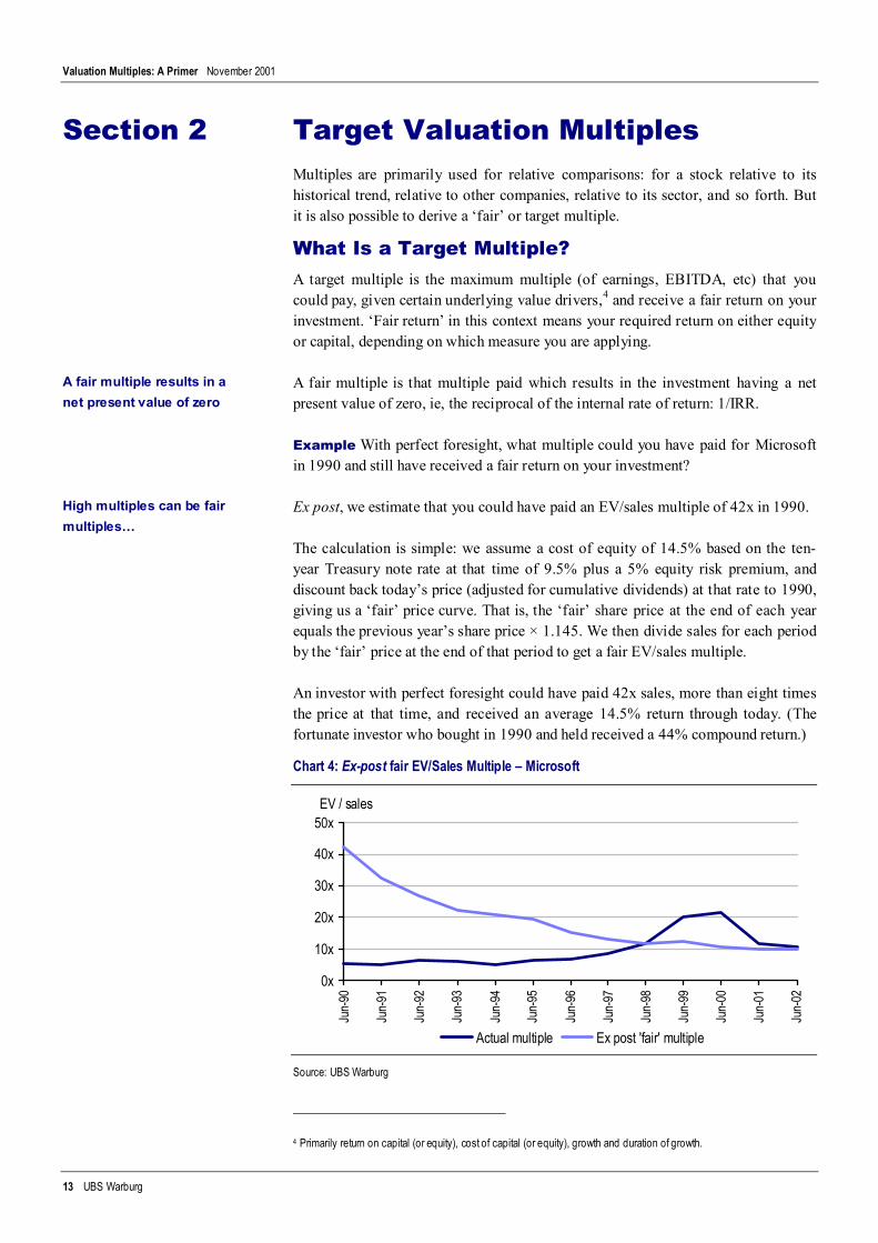
Example With perfect foresight, what multiple could you have paid for Microsoftin 1990 and still have received a fair return on your investment?
Ex post, we estimate that you could have paid an EV/sales multiple of 42x in 1990.
The calculation is simple: we assume a cost of equity of 14.5% based on the ten-year Treasury note rate at that time of 9.5% plus a 5% equity risk premium, anddiscount back today’s price (adjusted for cumulative dividends) at that rate to 1990,giving us a ‘fair’ price curve. That is, the ‘fair’ share price at the end of each yearequals the previous year’s share price × 1.145. We then divide sales for each periodby the ‘fair’ price at the end of that period to get a fair EV/sales multiple.
An investor with perfect foresight could have paid 42x sales, more than eight timesthe price at that time, and received an average 14.5% return through today. (Thefortunate investor who bought in 1990 and held received a 44% compound return.)
Chart 4: Ex-post fair EV/Sales Multiple – Microsoft
0x
10x
20x
30x
40x
50x
Jun-
90
Jun-
91
Jun-
92
Jun-
93
Jun-
94
Jun-
95
Jun-
96
Jun-
97
Jun-
98
Jun-
99
Jun-
00
Jun-
01
Jun-
02EV / sales
Actual multiple Ex post 'fair' multiple
Source: UBS Warburg
4 Primarily return on capital (or equity), cost of capital (or equity), growth and duration of growth.
Section 2
A fair multiple results in anet present value of zero
High multiples can be fairmultiples…
Valuation Multiples: A Primer November 2001
14 UBS Warburg
We do not need to know what the actual value drivers were in order to estimate aretrospective fair multiple, as we can work backward from a known share price.
But it is precisely those value drivers – particularly Microsoft’s high return oncapital and high growth rate requiring minimal reinvestment – that drove the shareprice. In 1990 Microsoft’s future success was neither apparent nor impounded in theshare price. But an investor who did see Microsoft’s potential and translated thatpotential into value driver estimates would have been willing to pay a much highermultiple.
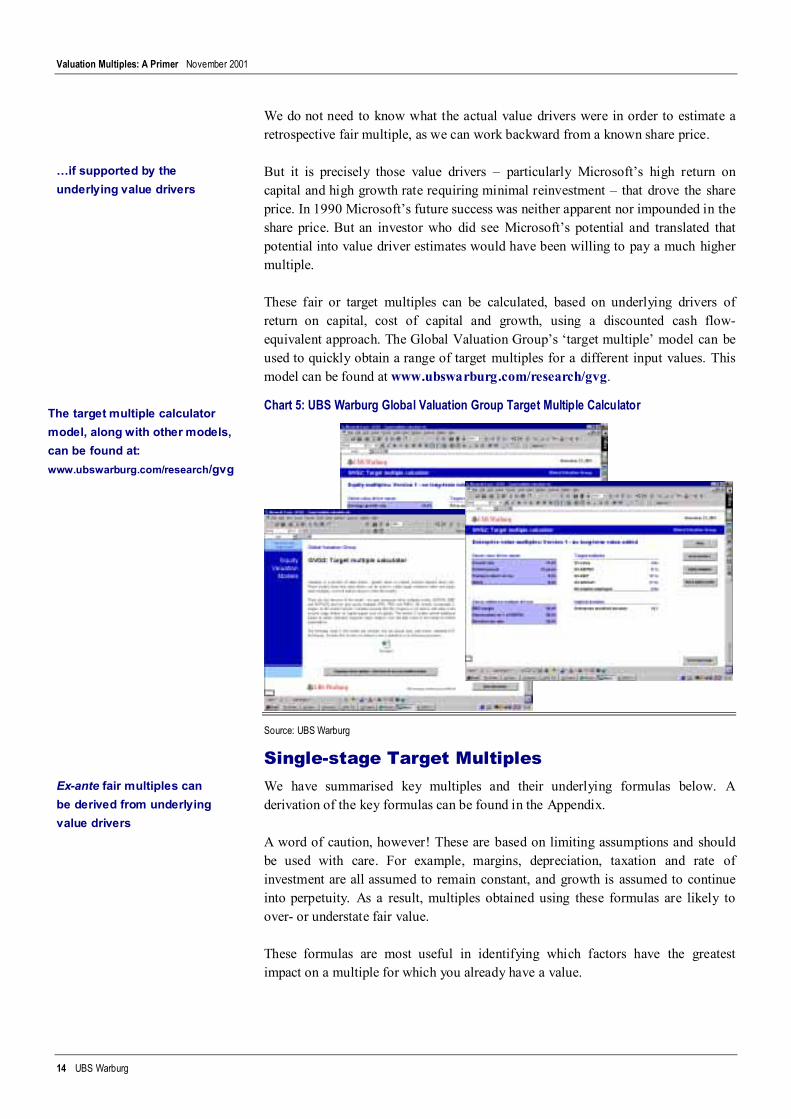
These fair or target multiples can be calculated, based on underlying drivers ofreturn on capital, cost of capital and growth, using a discounted cash flow-equivalent approach. The Global Valuation Group’s ‘target multiple’ model can beused to quickly obtain a range of target multiples for a different input values. Thismodel can be found at www.ubswarburg.com/research/gvg.
Chart 5: UBS Warburg Global Valuation Group Target Multiple Calculator
Source: UBS Warburg
Single-stage Target MultiplesWe have summarised key multiples and their underlying formulas below. Aderivation of the key formulas can be found in the Appendix.
A word of caution, however! These are based on limiting assumptions and shouldbe used with care. For example, margins, depreciation, taxation and rate ofinvestment are all assumed to remain constant, and growth is assumed to continueinto perpetuity. As a result, multiples obtained using these formulas are likely toover- or understate fair value.
These formulas are most useful in identifying which factors have the greatestimpact on a multiple for which you already have a value.
…if supported by theunderlying value drivers
The target multiple calculatormodel, along with other models,can be found at:www.ubswarburg.com/research/gvg
Ex-ante fair multiples canbe derived from underlyingvalue drivers
Valuation Multiples: A Primer November 2001
15 UBS Warburg
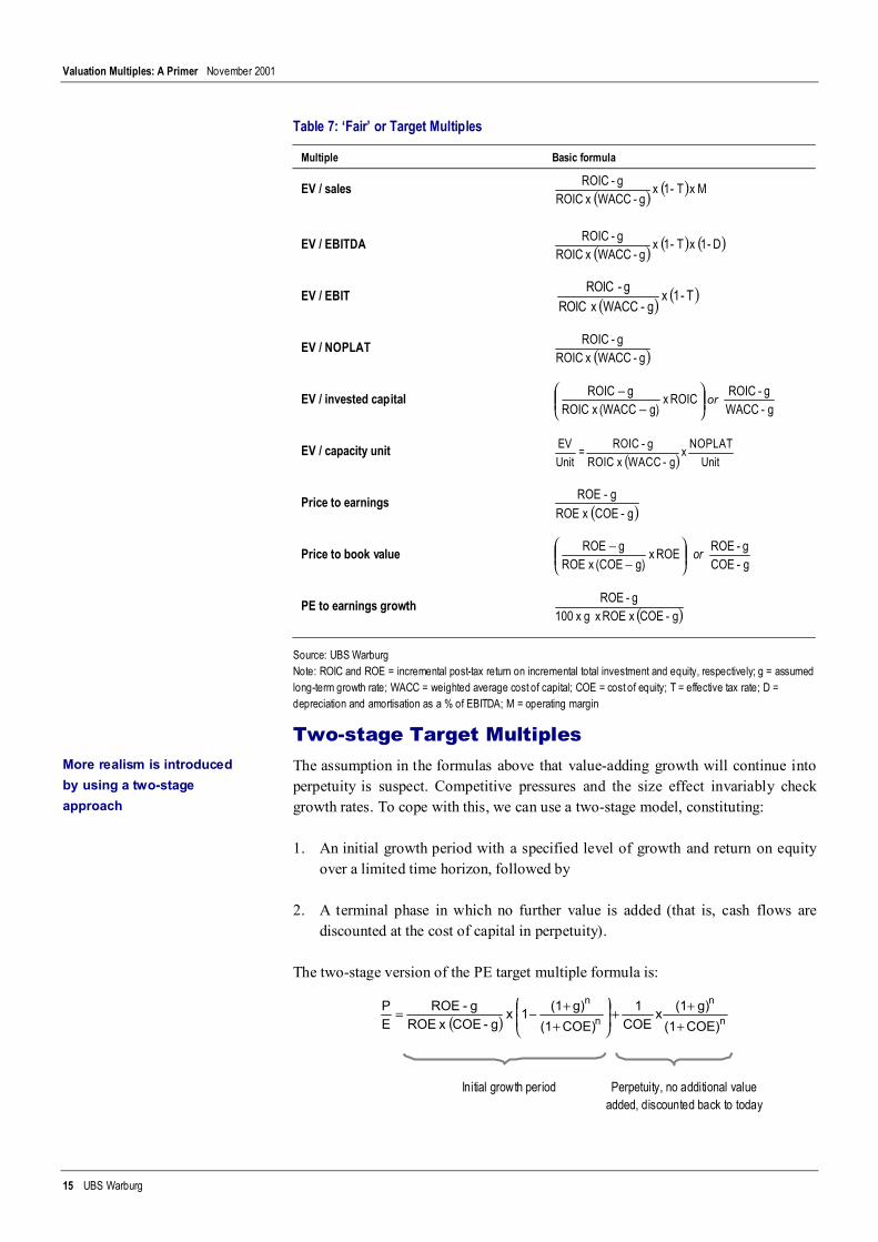
Table 7: ‘Fair’ or Target Multiples
Multiple Basic formula
EV / sales ( ) ( ) M xT - 1 xg - WACC xROIC
g - ROIC
EV / EBITDA ( ) ( ) ( )D - 1 xT - 1 xg - WACC xROIC
g - ROIC
EV / EBIT ( ) ( )T - 1 xg - WACC xROIC
g - ROIC
EV / NOPLAT ( )g - WACC xROICg - ROIC
EV / invested capital
−
− ROIC xg)(WACC xROIC
gROICor
g- WACCg - ROIC
EV / capacity unit ( ) UnitNOPLATx
g - WACC xROICg - ROIC =
UnitEV
Price to earnings ( )g -COE xROEg - ROE
Price to book value
−
− ROE xg)(COE xROE
gROE or g- COEg - ROE
PE to earnings growth ( ) g -COE xROE xg x100g - ROE
Source: UBS WarburgNote: ROIC and ROE = incremental post-tax return on incremental total investment and equity, respectively; g = assumedlong-term growth rate; WACC = weighted average cost of capital; COE = cost of equity; T = effective tax rate; D =depreciation and amortisation as a % of EBITDA; M = operating margin
Two-stage Target MultiplesThe assumption in the formulas above that value-adding growth will continue intoperpetuity is suspect. Competitive pressures and the size effect invariably checkgrowth rates. To cope with this, we can use a two-stage model, constituting:
1. An initial growth period with a specified level of growth and return on equityover a limited time horizon, followed by
2. A terminal phase in which no further value is added (that is, cash flows arediscounted at the cost of capital in perpetuity).
The two-stage version of the PE target multiple formula is:
( ) n
n
n
n
COE)(1g)(1x
COE1
COE)(1g)(11 x
g -COE x ROEg - ROE
EP
+++
++−=
More realism is introducedby using a two-stageapproach
Initial growth period Perpetuity, no additional valueadded, discounted back to today
Valuation Multiples: A Primer November 2001
16 UBS Warburg
Two-stage formulas are used in the Global Valuation Group (GVG) target multiplemodel. The derivation of the two-stage formula can be found in the Appendix.
Examples■■■■ Simple model, no value added: Suppose you are in investor with a required
return on equity (cost of equity) of 10%, contemplating investing in a companywith a return on equity of 10% and a growth rate of 5% into perpetuity. There isno value added (that is, the company does not generate any surplus return aboveyour cost of equity), and therefore the rate of growth is irrelevant. Thisinvestment is identical to a bond paying 10% in perpetuity, and the maximumyou would pay is (1/.10) or 10x the coupon. The fair PE multiple is 10xregardless of the company’s growth rate.
■■■■ Simple model, value added: Now consider a company with a return on equityof 12% and a growth rate of 5% to perpetuity. Because the company generates areturn above your cost of equity, you will pay a higher PE ratio; the higher thegrowth rate, the more value added and the higher the PE you will pay. The fairPE ratio in this instance is:
12x.05) - (.10 .12
.05 - .12EP ==
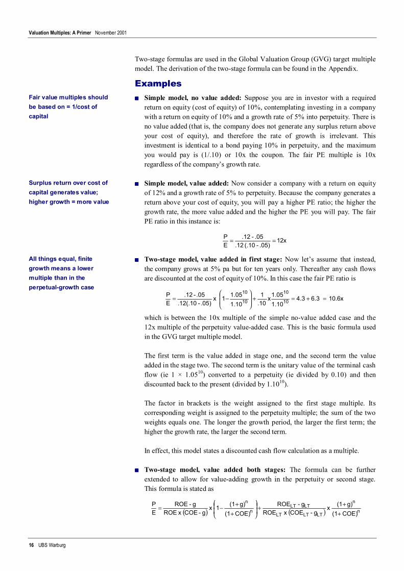
■■■■ Two-stage model, value added in first stage: Now let’s assume that instead,the company grows at 5% pa but for ten years only. Thereafter any cash flowsare discounted at the cost of equity of 10%. In this case the fair PE ratio is
10.6x 6.3 4.31.101.05x
.101
1.101.051 x
.05)-.12(.10.05-.12
EP
10
10
10
10=+=+
−=
which is between the 10x multiple of the simple no-value added case and the12x multiple of the perpetuity value-added case. This is the basic formula usedin the GVG target multiple model.
The first term is the value added in stage one, and the second term the valueadded in the stage two. The second term is the unitary value of the terminal cashflow (ie 1 × 1.0510) converted to a perpetuity (ie divided by 0.10) and thendiscounted back to the present (divided by 1.1010).
The factor in brackets is the weight assigned to the first stage multiple. Itscorresponding weight is assigned to the perpetuity multiple; the sum of the twoweights equals one. The longer the growth period, the larger the first term; thehigher the growth rate, the larger the second term.
In effect, this model states a discounted cash flow calculation as a multiple.
■■■■ Two-stage model, value added both stages: The formula can be furtherextended to allow for value-adding growth in the perpetuity or second stage.This formula is stated as
( ) ( ) COE)(1
g)(1 x g -COE x ROE
g - ROE COE)(1
g)(11 x g -COE x ROE
g - ROEEP
n
n
LTLTLT
LTLTn
n
+++
++−=
Fair value multiples shouldbe based on = 1/cost ofcapital
Surplus return over cost ofcapital generates value;higher growth = more value
All things equal, finitegrowth means a lowermultiple than in theperpetual-growth case
Valuation Multiples: A Primer November 2001
17 UBS Warburg
where ROELT = the long-term return on equity, COELT = the investor’s long-termrequired return on equity and gLT = the long-term (steady state) growth rate.
Note that the discount factor in the final term is based on the first-stage growthrate and cost of equity. The numerator grosses up the current unitary cash flow(that is, 1) to a terminal cash flow at the end of the initial growth period, usingthe initial-period growth rate. This is then multiplied by a cash flow exitmultiple (the PE formula using long-term value drivers) to give us the terminalvalue at the end of the first stage. This terminal value is then discounted back totoday using the current cost of equity.
In other words, the two terms of the equation are equivalent to the explicitforecast period and terminal value in a discounted cash flow calculation.
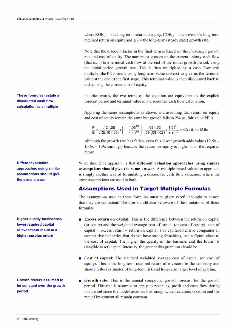
Applying the same assumptions as above, and assuming that return on equityand cost of equity remain the same but growth falls to 2% pa, fair value PE is:
( ) 12.5x8.14.3 1.101.05 x
.02-.08 .09.02- .09
1.101.051 x
.05)-.12(.10.05-.12
EP
10
10
10
10=+=+
−=
Although the growth rate has fallen, even this lower growth adds value (12.5x –10.6x = 1.9x earnings) because the return on equity is higher than the requiredreturn.
What should be apparent is that different valuation approaches using similarassumptions should give the same answer. A multiple-based valuation approachis simply another way of formulating a discounted cash flow valuation, where thesame assumptions are used in both.
Assumptions Used in Target Multiple FormulasThe assumptions used in these formulas must be given careful thought to ensurethat they are consistent. The user should also be aware of the limitations of theseformulas.
■■■■ Excess return on capital: This is the difference between the return on capital(or equity) and the weighted average cost of capital (or cost of equity): cost ofcapital + excess return = return on capital. For capital-intensive companies incompetitive industries that do not have strong franchises, use a figure close tothe cost of capital. The higher the quality of the business and the lower its(tangible asset) capital intensity, the greater this premium should be.
■■■■ Cost of capital: The standard weighted average cost of capital (or cost ofequity). This is the long-term required return of investors in the company andshould reflect estimates of long-term risk and long-term target level of gearing.
■■■■ Growth rate: This is the annual compound growth forecast for the growthperiod. This rate is assumed to apply to revenues, profit and cash flow duringthis period since the model assumes that margins, depreciation, taxation and therate of investment all remain constant.
These formulas restate adiscounted cash flowcalculation as a multiple
Different valuationapproaches using similarassumptions should givethe same answer
Higher quality businesses/lower required capitalreinvestment result in ahigher surplus return
Growth drivers assumed tobe constant over the growthperiod
Valuation Multiples: A Primer November 2001
18 UBS Warburg
■■■■ Growth period: The estimated period over which the initial growth rate and theexcess return on capital are expected to persist. In the simpler version of themodel, it is assumed that at the end of the initial growth period the excess returnon capital changes to zero (in the GVG target multiple model this can bemodified in the two-stage model for which value is added in both stages).
The Effect of Growth on ValueIf asked which value driver has the greatest impact on multiples, analysts andinvestors are likely to answer ‘growth’. This is broadly true, but the impact ofgrowth depends on its source and nature. There are several different sources ofgrowth and each will have a different effect on value creation and thus share prices.
The four primary sources of growth are:
■■■■ Growth due to reinvestment at the cost of capital
■■■■ Growth due to reinvestment at a premium to the cost of capital
■■■■ Growth due to inflation
■■■■ Growth due to efficiency gains5
Reinvestment at the cost of capital Growth as a result of reinvestment at thecost of capital does not add value, and neither the share price nor the PE ratio isaffected. In this case the PE formula reduces to:
COE1
Reinvestment at a premium to the cost of capital Growth as a result ofreinvestment at an incremental return higher than the cost of capital will producevalue-adding growth. (Conversely, if the company reinvests at an incrementalreturn that is below the cost of capital, value is destroyed.) The formula is the sameas that for the single-stage PE target multiple discussed above:
( )g -COE x ROEg - ROE
Inflationary growth Growth resulting from a general increase in the price level(which produces higher earnings) results in a lower multiple (although notnecessarily lower value, because of the higher nominal value of earnings). This isbecause the replacement value of fixed assets and working capital rises, requiringmore investment to fund that increase in value.
( )rrr
rrg -COE x ) (ROE
g - ROE∏+
The subscript ‘r’ denotes real rather than nominal. П = inflation
Efficiency gains Productivity gains not requiring additional investment, such asthose resulting from cost control or higher market share, are a valuable source ofgrowth. Even small gains can produce large increases in the PE ratio.
5 For a more detailed discussion of the impact of growth on multiples, see our report Price Earnings Growth: A PEG forYour Valuations, November 1997, available at ubswarburg.com/research/gvg.
Growth is seen to have thegreatest impact on value…
…but this depends on thesource of growth
Reinvestment may or maynot add value depending onexcess return on capital
Inflation-driven growthresults in a lower multiple
Efficiency gains can be avaluable source of growth

Valuation Multiples: A Primer November 2001
19 UBS Warburg
( ) g -COE x ROEg - (g - ROE eff )
g = total forecast growth; geff = growth achieved from efficiency gains
Implicit in the above formula is the assumption that efficiency gains are achieved inperpetuity. Because efficiency gains are likely to be eroded fairly quickly, a morerealistic multiple would lie between this multiple and the fair value PE ratio underan assumption of normal reinvestment.
The chart shows sensitivity of multiples to growth rates for different growth types.
Chart 6: Effect of Different Sources of Growth on the PE Ratio
0x
10x
20x
30x
40x
50x
0% 1% 2% 3% 4% 5%Earnings growth rate
PE ratio
(1) Efficiency gains (2) ROE > COE (3) ROE = COE(4) Inflation only (5) ROE < COE
Source: UBS WarburgNote: Assumes perpetual growth arising from: (1) perpetual efficiency gains = the long-term growth rate; (2) and (5)reinvestment at a 3% premium/discount to COE; (3) reinvestment at COE; (4) inflationary growth only
In reality efficiency gainsare likely to be erodedquickly
Valuation Multiples: A Primer November 2001
20 UBS Warburg
Using Valuation MultiplesRelative Valuation – Observed Multiple versus ComparableThere are several ways one can apply multiples in valuation. The common approachis to compare the current multiple to a historical multiple measured at a comparablepoint in the business cycle and macroeconomic environment. An alternate approachis to compare current multiples to those of other companies, a sector or a market,and compare the current spread between them to a historical spread.
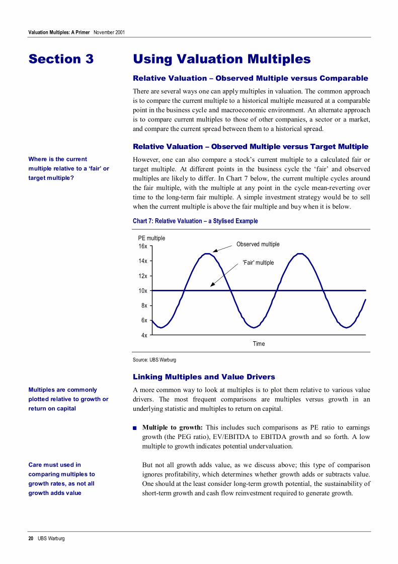
Relative Valuation – Observed Multiple versus Target MultipleHowever, one can also compare a stock’s current multiple to a calculated fair ortarget multiple. At different points in the business cycle the ‘fair’ and observedmultiples are likely to differ. In Chart 7 below, the current multiple cycles aroundthe fair multiple, with the multiple at any point in the cycle mean-reverting overtime to the long-term fair multiple. A simple investment strategy would be to sellwhen the current multiple is above the fair multiple and buy when it is below.
Chart 7: Relative Valuation – a Stylised Example
4x
6x
8x
10x
12x
14x
16x
Time
PE multipleObserved multiple
'Fair' multiple
Source: UBS Warburg
Linking Multiples and Value DriversA more common way to look at multiples is to plot them relative to various valuedrivers. The most frequent comparisons are multiples versus growth in anunderlying statistic and multiples to return on capital.
■■■■ Multiple to growth: This includes such comparisons as PE ratio to earningsgrowth (the PEG ratio), EV/EBITDA to EBITDA growth and so forth. A lowmultiple to growth indicates potential undervaluation.
But not all growth adds value, as we discuss above; this type of comparisonignores profitability, which determines whether growth adds or subtracts value.One should at the least consider long-term growth potential, the sustainability ofshort-term growth and cash flow reinvestment required to generate growth.
Section 3
Where is the currentmultiple relative to a ‘fair’ ortarget multiple?
Multiples are commonlyplotted relative to growth orreturn on capital
Care must used incomparing multiples togrowth rates, as not allgrowth adds value
Valuation Multiples: A Primer November 2001
21 UBS Warburg
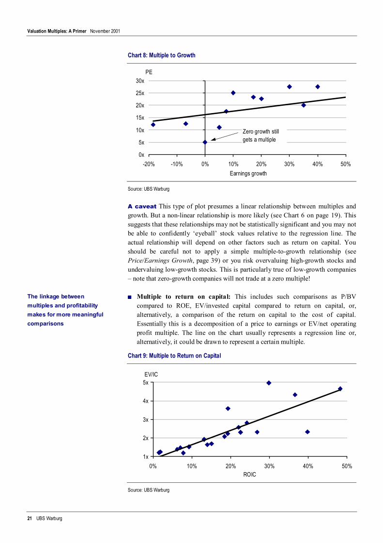
Chart 8: Multiple to Growth
0x
5x
10x
15x
20x
25x
30x
-20% -10% 0% 10% 20% 30% 40% 50%Earnings growth
PE
Zero growth still gets a multiple
Source: UBS Warburg
A caveat This type of plot presumes a linear relationship between multiples andgrowth. But a non-linear relationship is more likely (see Chart 6 on page 19). Thissuggests that these relationships may not be statistically significant and you may notbe able to confidently ‘eyeball’ stock values relative to the regression line. Theactual relationship will depend on other factors such as return on capital. Youshould be careful not to apply a simple multiple-to-growth relationship (seePrice/Earnings Growth, page 39) or you risk overvaluing high-growth stocks andundervaluing low-growth stocks. This is particularly true of low-growth companies– note that zero-growth companies will not trade at a zero multiple!
■■■■ Multiple to return on capital: This includes such comparisons as P/BVcompared to ROE, EV/invested capital compared to return on capital, or,alternatively, a comparison of the return on capital to the cost of capital.Essentially this is a decomposition of a price to earnings or EV/net operatingprofit multiple. The line on the chart usually represents a regression line or,alternatively, it could be drawn to represent a certain multiple.
Chart 9: Multiple to Return on Capital
1x
2x
3x
4x
5x
0% 10% 20% 30% 40% 50%ROIC
EV/IC
Source: UBS Warburg
The linkage betweenmultiples and profitabilitymakes for more meaningfulcomparisons
Valuation Multiples: A Primer November 2001
22 UBS Warburg
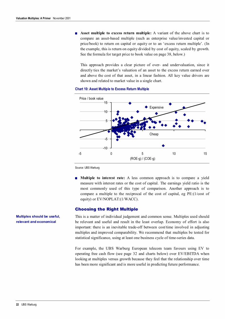
■■■■ Asset multiple to excess return multiple: A variant of the above chart is tocompare an asset-based multiple (such as enterprise value/invested capital orprice/book) to return on capital or equity or to an ‘excess return multiple’. (Inthe example, this is return on equity divided by cost of equity, scaled by growth.See the formula for target price to book value on page 38, below.)
This approach provides a clear picture of over- and undervaluation, since itdirectly ties the market’s valuation of an asset to the excess return earned overand above the cost of that asset, in a linear fashion. All key value drivers areshown and related to market value in a single chart.
Chart 10: Asset Multiple to Excess Return Multiple
-10
-5
-
5
10
15
-5 0 5 10 15(ROE-g) / (COE-g)
Price / book value
Expensive
Cheap
Source: UBS Warburg
■■■■ Multiple to interest rate: A less common approach is to compare a yieldmeasure with interest rates or the cost of capital. The earnings yield ratio is themost commonly used of this type of comparison. Another approach is tocompare a multiple to the reciprocal of the cost of capital, eg PE:(1/cost ofequity) or EV/NOPLAT:(1/WACC).
Choosing the Right MultipleThis is a matter of individual judgement and common sense. Multiples used shouldbe relevant and useful and result in the least overlap. Economy of effort is alsoimportant: there is an inevitable trade-off between cost/time involved in adjustingmultiples and improved comparability. We recommend that multiples be tested forstatistical significance, using at least one business cycle of time-series data.
For example, the UBS Warburg European telecom team favours using EV tooperating free cash flow (see page 32 and charts below) over EV/EBITDA whenlooking at multiples versus growth because they feel that the relationship over timehas been more significant and is more useful in predicting future performance.
Multiples should be useful,relevant and economical

Valuation Multiples: A Primer November 2001
23 UBS Warburg
Chart 11: European Telecom Sector – ‘babycoms’ – EV/EBITDA Chart 12: European Telecom Sector – ‘babycoms’ – EV/OpFCF
R2 = 0.069
0x
5x
10x
15x
20x
0% 5% 10% 15% 20% 25% 30% 35% 40%EBITDA CAGR 01E-04E
EV / EBITDA R2 = 0.7235
0x
25x
50x
75x
100x
0% 20% 40% 60% 80% 100% 120% 140% 160% 180% 200%OpFCF CAGR 01E-04E
EV / OpFCF
Source: UBS Warburg Source: UBS Warburg
Valuation Multiples: A Primer November 2001
24 UBS Warburg
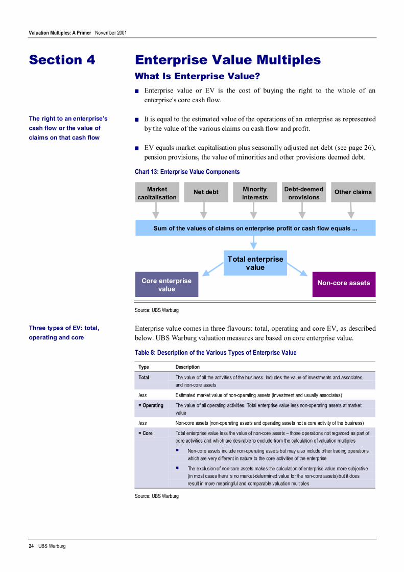
Enterprise Value MultiplesWhat Is Enterprise Value?■■■■ Enterprise value or EV is the cost of buying the right to the whole of an
enterprise's core cash flow.
■■■■ It is equal to the estimated value of the operations of an enterprise as representedby the value of the various claims on cash flow and profit.
■■■■ EV equals market capitalisation plus seasonally adjusted net debt (see page 26),pension provisions, the value of minorities and other provisions deemed debt.
Chart 13: Enterprise Value Components
Source: UBS Warburg
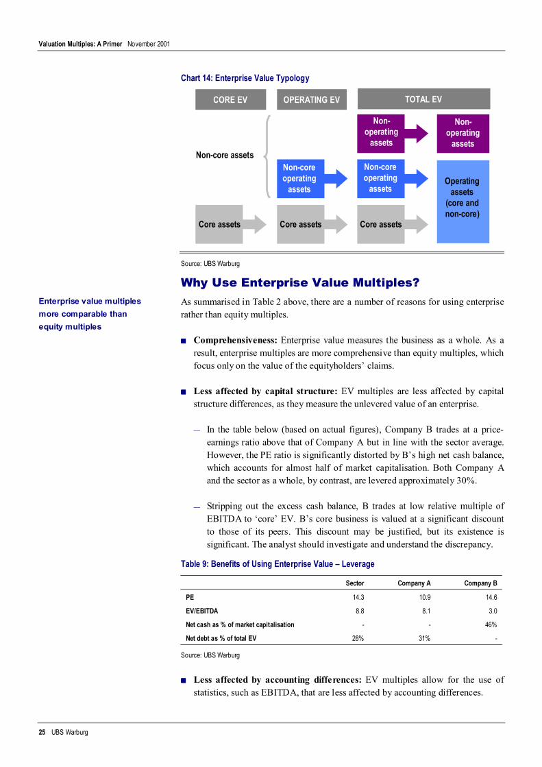
Enterprise value comes in three flavours: total, operating and core EV, as describedbelow. UBS Warburg valuation measures are based on core enterprise value.
Table 8: Description of the Various Types of Enterprise Value
Type Description
Total The value of all the activities of the business. Includes the value of investments and associates,and non-core assets
less Estimated market value of non-operating assets (investment and usually associates)
= Operating The value of all operating activities. Total enterprise value less non-operating assets at marketvalue
less Non-core assets (non-operating assets and operating assets not a core activity of the business)
= Core Total enterprise value less the value of non-core assets – those operations not regarded as part ofcore activities and which are desirable to exclude from the calculation of valuation multiples
Non-core assets include non-operating assets but may also include other trading operationswhich are very different in nature to the core activities of the enterprise
The exclusion of non-core assets makes the calculation of enterprise value more subjective(in most cases there is no market-determined value for the non-core assets) but it doesresult in more meaningful and comparable valuation multiples
Source: UBS Warburg
Section 4
The right to an enterprise'scash flow or the value ofclaims on that cash flow
Three types of EV: total,operating and core
Marketcapitalisation
Minorityinterests
Other claimsNet debt Debt-deemedprovisions
Sum of the values of claims on enterprise profit or cash flow equals ...
Total enterprisevalue
Core enterprisevalue
Non-core assets
Valuation Multiples: A Primer November 2001
25 UBS Warburg
Chart 14: Enterprise Value Typology
Source: UBS Warburg
Why Use Enterprise Value Multiples?As summarised in Table 2 above, there are a number of reasons for using enterpriserather than equity multiples.
■■■■ Comprehensiveness: Enterprise value measures the business as a whole. As aresult, enterprise multiples are more comprehensive than equity multiples, whichfocus only on the value of the equityholders’ claims.
■■■■ Less affected by capital structure: EV multiples are less affected by capitalstructure differences, as they measure the unlevered value of an enterprise.
— In the table below (based on actual figures), Company B trades at a price-earnings ratio above that of Company A but in line with the sector average.However, the PE ratio is significantly distorted by B’s high net cash balance,which accounts for almost half of market capitalisation. Both Company Aand the sector as a whole, by contrast, are levered approximately 30%.
— Stripping out the excess cash balance, B trades at low relative multiple ofEBITDA to ‘core’ EV. B’s core business is valued at a significant discountto those of its peers. This discount may be justified, but its existence issignificant. The analyst should investigate and understand the discrepancy.
Table 9: Benefits of Using Enterprise Value – Leverage
Sector Company A Company B
PE 14.3 10.9 14.6
EV/EBITDA 8.8 8.1 3.0
Net cash as % of market capitalisation - - 46%
Net debt as % of total EV 28% 31% -
Source: UBS Warburg
■■■■ Less affected by accounting differences: EV multiples allow for the use ofstatistics, such as EBITDA, that are less affected by accounting differences.
Enterprise value multiplesmore comparable thanequity multiples
Non-operating
assets
Operatingassets
(core andnon-core)
Core assets Core assets
Non-coreoperating
assets
Non-coreoperating
assets
Core assets
Non-operating
assets
CORE EV OPERATING EV TOTAL EV
Non-core assets

Valuation Multiples: A Primer November 2001
26 UBS Warburg
■■■■ Less distorted by non-core assets: EV multiples allow the exclusion of non-core assets, whereas the statistics used in equity multiples incorporate the netassets and earnings attributable to non-core assets.
As a result, enterprise value multiples are more comparable among companies thanequity multiples.
Potential Problems in Calculating EVA number of potential problems arise in the calculation of enterprise value.6
■■■■ Is enterprise value complete?
■■■■ Is enterprise value measured at market values?
■■■■ Does net debt reflect seasonal variations and changes in group composition?
■■■■ Have non-operating and non-core assets been treated correctly?
1. CompletenessEnterprise value should include all claims on the company, not just marketcapitalisation and net debt. This includes claims relating to deemed debt (provisionshaving the characteristics of interest-bearing debt, such as unfunded pensionliabilities), options, preferred shareholdings and minority interests.
2. Use of Market ValuesEnterprise value should include the value of claims at market, not book values. Debtshould be adjusted to reflect market value. Minority shares in a subsidiary should bequoted at market value; otherwise a valuation multiple should be applied toearnings or net assets. Quoted options should be valued at market and, whereunquoted, at fair value ideally, or as a minimum at intrinsic value.
3. SeasonalityEV should reflect an average level of debt which is adjusted to reflect seasonalvariations and for changes in the composition of the group. This is important, as netdebt is usually the largest component of EV after market capitalisation, and usingthe stated balance sheet amount can result in large errors.
4. Treatment of Non-operating and Non-core AssetsNon-operating assets are investments and other activities that do not form part ofthe firm’s trading (day-to-day business) operations. Non-core assets include non-operating and any other trading activities that are so different in nature that failureto exclude them from core EV would seriously distort multiples. Income producedby non-core assets is not part of core EBIT.
Non-operating assets typically include net cash balances, other investments and,usually, associates. Non-operating associates should be deducted from total
6 For a more detailed discussion of issues involved in calculating enterprise value, see our report Valuation andAccounting Briefing No. 1: Enterprise Value, December 1998 (reprinted November 2000), available atubswarburg.com/research/gvg.
EV calculations have pitfallsfor the unwary
EV should include all claimson the company, not justmarket cap and net debt
EV should reflect anaverage level of net debt
Valuation Multiples: A Primer November 2001
27 UBS Warburg
enterprise value at market value (if necessary, estimated by applying a groupearnings multiple to the group’s share of associate income).
But associates may straddle the operating/non-operating line. Where associates areconsidered part of operating activities, this can lead to problems with multiples:
■■■■ If the post-interest profit of the associate is included in EBIT then the result is amixed multiple, with both pre- and post-interest earnings combined in thedenominator.
■■■■ But if the associate profit included in EBIT is pre-interest – this is not oftenavailable in accounts – then the parent share of associate net debt should beincluded in the parent’s enterprise value.
■■■■ In calculating EBITDA multiples, the group’s share of associate depreciationand amortisation must be added back to EBITDA.
It is generally best to treat associates as non-operating assets (effectivelyinvestments) in calculating operating and core enterprise value. This meansexcluding the associate share of profit from core and operating EBIT (thus therespective multiples are core EV/core EBIT and operating EV/operating EBIT).
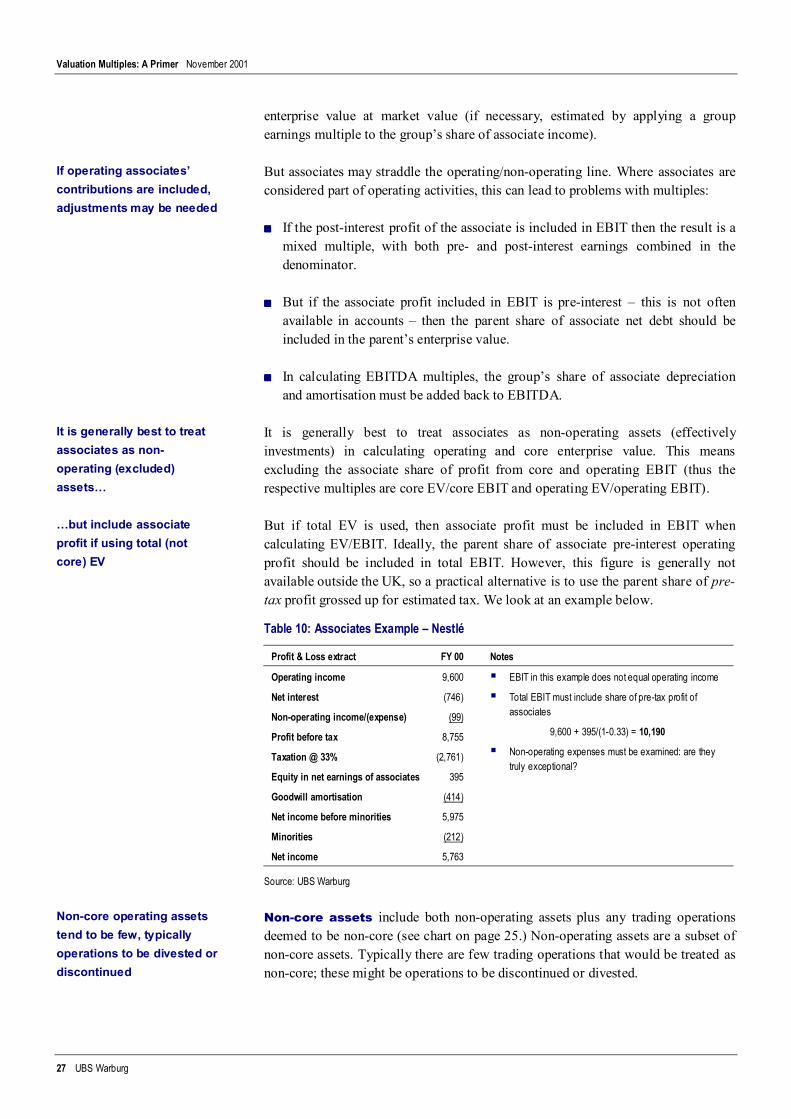
But if total EV is used, then associate profit must be included in EBIT whencalculating EV/EBIT. Ideally, the parent share of associate pre-interest operatingprofit should be included in total EBIT. However, this figure is generally notavailable outside the UK, so a practical alternative is to use the parent share of pre-tax profit grossed up for estimated tax. We look at an example below.
Table 10: Associates Example – Nestlé
Profit & Loss extract FY 00 Notes
Operating income
Net interest
Non-operating income/(expense)
Profit before tax
Taxation @ 33%
Equity in net earnings of associates
Goodwill amortisation
Net income before minorities
Minorities
Net income
9,600
(746)
(99)
8,755
(2,761)
395
(414)
5,975
(212)
5,763
EBIT in this example does not equal operating income
Total EBIT must include share of pre-tax profit ofassociates
9,600 + 395/(1-0.33) = 10,190
Non-operating expenses must be examined: are theytruly exceptional?
Source: UBS Warburg
Non-core assets include both non-operating assets plus any trading operationsdeemed to be non-core (see chart on page 25.) Non-operating assets are a subset ofnon-core assets. Typically there are few trading operations that would be treated asnon-core; these might be operations to be discontinued or divested.
If operating associates’contributions are included,adjustments may be needed
It is generally best to treatassociates as non-operating (excluded)assets…
…but include associateprofit if using total (notcore) EV
Non-core operating assetstend to be few, typicallyoperations to be divested ordiscontinued
Valuation Multiples: A Primer November 2001
28 UBS Warburg
Enterprise Value MultiplesThere are many different enterprise value multiples that can be calculated,depending on the circumstances. What is most important is that the denominatorrepresent a flow to all claimants on enterprise cash flow.
Adjustments should be made to both enterprise value and the denominator wherenecessary (and possible) to ensure that apples are being compared with apples.
EV/SalesDefinition: Core EV/sales.
Formula: ( ) ( ) M x T - 1 x g - WACC x ROIC
g - ROIC = SalesEV
When to use it
■■■■ EV/sales is a crude measure, but least susceptible to accounting differences; it isequivalent to its equity counterpart, price to sales, where a company has no debt.
■■■■ EV/sales is useful when accounting differences among comparables are extreme,or where profit or cash flow figures are unrepresentative or negative. It isfrequently used for unprofitable or cyclical firms where there are problems inmeasuring profit or cash flow further down the P&L. As a proxy for cash flow,sales has the virtue of being stable and relatively unaffected by accountingpolicies.
■■■■ EV/sales is also useful in identifying restructuring potential. Net margin is a keydriver of this measure; low profitability (low net margin) would result in a lowvalue for a given level of sales.
■■■■ Be careful that the sales figure is representative; generally EV/sales should notbe used for companies with variable, periodic sales, such as property developers.
Caveats There are three caveats in using this multiple:
■■■■ Sales volatility: EV/sales is frequently applied to technology firms, which arelikely to have negative cash flow and/or earnings while they are in their initialgrowth phase. But these companies frequently have highly volatile sales as well.
■■■■ Revenue recognition policies: Sales are not unaffected by accounting policies.Sales can be substantially affected by different interpretations of accountingstandards in such areas as:
— Use of gross versus net revenue in recording sales on agency transactions
— Treatment of sales where a customer has the right of return
— Long-term contracts accounted for under percentage of completion orcompleted contract methods
The multiple denominatormust represent a flow to allclaimants
Crude but least susceptibleto accounting differences
Useful in identifyingrestructuring potential
Sales can be affected byaccounting policies
Valuation Multiples: A Primer November 2001
29 UBS Warburg
Care must be taken in ensuring that, when making comparisons using thismultiple, sales are determined on a consistent basis.
■■■■ Margin differences. Sales multiples cannot be directly compared acrossbusinesses where operating margins differ. Rough comparability can be obtainby adjusting the sales multiple to
margin operatingcompany Benchmarkmultiple) salescompany (target multiple) salescompany (Benchmark x
where the target company is the one being valued.
EV/EBITDADefinition: Core EV/earnings before associates, interest, tax, depreciation,amortisation, non-cash changes in provisions and before reported exceptional items.
Formula: ( ) ( ) ( )D - 1 x T - 1 x g - WACC x ROIC
g - ROIC = EBITDA
EV
When to use it
■■■■ EBITDA is a proxy for operating cash flow, and EV/EBITDA – probably themost popular EV multiple – is a price to cash flow multiple. Its popularity stemsfrom the fact that it is unaffected by differences in depreciation policy andappears unaffected by differences in capital structure.
■■■■ However, while EBITDA is closer to cash flow than other profit measures it isnot a true cash flow, as it does not incorporate either asset depreciation or capitalexpenditure. Also, EBITDA is a pretax measure, whereas management canpotentially add value through skilled tax management.
■■■■ EV/EBITDA is affected by a firm’s level of capital intensity (measured asdepreciation as a percentage of EBITDA). All things being equal, higher capitalintensity results in a lower EV/EBITDA multiple.7
7 For further discussion, see our report Valuation and Accounting Briefing No. 3: EBITDA Multiples and Capital Intensity,February 1999, available at ubswarburg.com/research/gvg.
Sales multiples cannot becompared where operatingmargins differ
EBITDA does not includethe cost of replacing capital
Valuation Multiples: A Primer November 2001
30 UBS Warburg
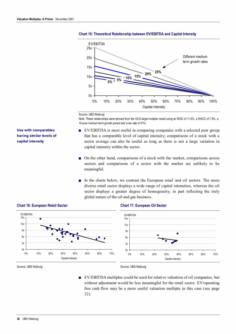
Chart 15: Theoretical Relationship between EV/EBITDA and Capital Intensity
0x
5x
10x
15x
20x
25x
0% 10% 20% 30% 40% 50% 60% 70% 80% 90% 100%Capital intensity
EV/EBITDA
0% 5% 10% 15% 20% 25%
Different medium term growth rates
Source: UBS WarburgNote: These relationships were derived from the GVG target multiple model using an ROIC of 11.5%, a WACC of 7.5%, a10-year medium-term growth period and a tax rate of 31%.
■■■■ EV/EBITDA is most useful in comparing companies with a selected peer groupthat has a comparable level of capital intensity; comparisons of a stock with asector average can also be useful as long as there is not a large variation incapital intensity within the sector.
■■■■ On the other hand, comparisons of a stock with the market, comparisons acrosssectors and comparisons of a sector with the market are unlikely to bemeaningful.
■■■■ In the charts below, we contrast the European retail and oil sectors. The morediverse retail sector displays a wide range of capital intensities, whereas the oilsector displays a greater degree of homogeneity, in part reflecting the trulyglobal nature of the oil and gas business.
Chart 16: European Retail Sector Chart 17: European Oil Sector
0x
3x
6x
9x
12x
15x
0% 10% 20% 30% 40% 50% 60% 70%Capital intensity
EV/EBITDA
0x
3x
6x
9x
12x
15x
0% 10% 20% 30% 40% 50% 60% 70%Capital intensity
EV/EBITDA
Source: UBS Warburg Source: UBS Warburg
■■■■ EV/EBITDA multiples could be used for relative valuation of oil companies, butwithout adjustment would be less meaningful for the retail sector. EV/operatingfree cash flow may be a more useful valuation multiple in this case (see page32).
Use with comparableshaving similar levels ofcapital intensity
Valuation Multiples: A Primer November 2001
31 UBS Warburg
■■■■ EV/EBITDA cannot be used when current cash flow is negative. Use normalisedEBITDA, or a forward multiple, instead.
EV/EBITDefinition: Core EV/core earnings before goodwill amortisation (but afteramortisation of other intangibles), associates, interest and taxes. It is stated prereported exceptional or extraordinary items.
Alternatively, this multiple may be defined as total EV/total EBIT (instead of coreEV/core EBIT).
Formula: ( ) ( )T - 1 x g - WACC x ROIC
g - ROIC = EBITEV
When to use it
■■■■ EBIT is a post-goodwill figure. However, we believe that goodwill amortisationis not an economic charge and should properly be added back to operatingprofit.
■■■■ EBIT is a better measure of ‘free’ (post-maintenance capital spending) cash flowthan EBITDA, and is more comparable where capital intensities differ.
■■■■ EBIT is, however, affected by accounting policy differences for depreciation.EV/EBIT is most useful where there are relatively small differences inaccounting treatment of depreciation among comparables.
■■■■ Alternatively, you can normalise depreciation. The example below demonstrateshow a simple depreciation adjustment would work.
Table 11: Adjusting EBIT for Differing Depreciation Policies
Gross fixed assets 300 Unadjusted posttax EBIT 32
Depreciable life 10 Add back: excess depreciation 10
Actual depreciation (no salvage) -30 Adjusted posttax EBIT 42
Normal depreciable life 15
Normalised depreciation -20
Excess depreciation -10
Source: UBS WarburgNote: We have not adjusted net profit for the ‘additional’ tax that theoretically would be paid as a result of lowerdepreciation expense. First, depreciation for tax purposes is typically calculated separately from book depreciation.Second, tax is a real expense that cannot be affected by analytical adjustments.
■■■■ Note that the goodwill adjustment does not apply to financial statementsreported under US GAAP. Recently-published Financial Accounting Statement142, Goodwill and Other Intangible Assets, stipulates that effective 1 January2002 (for calendar year companies), goodwill is no longer to be amortised. 8
8 For a detailed discussion of goodwill and its treatment in equity valuation, as well as recent developments in accountingfor goodwill under US GAAP, see our report Equity Analysis InsideOut No. 3: Goodwill in Equity Analysis, July 2001,available at ubswarburg.com/research/gvg.
Most useful wherecomparables’ depreciationpolicies are similar
Valuation Multiples: A Primer November 2001
32 UBS Warburg
EV/NOPLATDefinition: Core EV/normal operating profit less adjusted tax.
NOPLAT is post-tax EBIT. However, as commonly used, NOPLAT (or NOPAT)refers to EBI after adjustments to accounting profit to better reflect economic profit.
Some adjustments include adding back goodwill amortisation, LIFO reserveincrease, implied interest expense on operating leases, increases in bad debt andcapitalised R&D, and the adjustment of reported tax to a cash basis.9
Formula: ( )g - WACC x ROICg - ROIC =
NOPLATEV
When to use it
■■■■ NOPLAT is a more sophisticated and complete form of EBIT that allows fordifferences in tax efficiency and effective tax rates. If the company were allequity-financed, NOPLAT would equal earnings.
■■■■ However, the calculation of NOPLAT introduces a measure of subjectivity. Thismakes it harder to compare to other parties’ calculations of NOPLAT.
■■■■ The NOPLAT multiple is effectively a degeared PE and is a perfectly reasonablestatistic to use provided it is measured on a consistent basis across companies.EV/NOPLAT can be used as a substitute for EV/EBIT.
EV/OpFCFDefinition: Core EV/operating free cash flow (OpFCF). ROIC is calculated usingOpFCF in the numerator.
OpFCF is core EBITDA less charges for capital usage and for the effect of inflationon working capital needs. OpFCF should be measured before goodwillamortisation. A calculation of operating free cash flow is shown below.
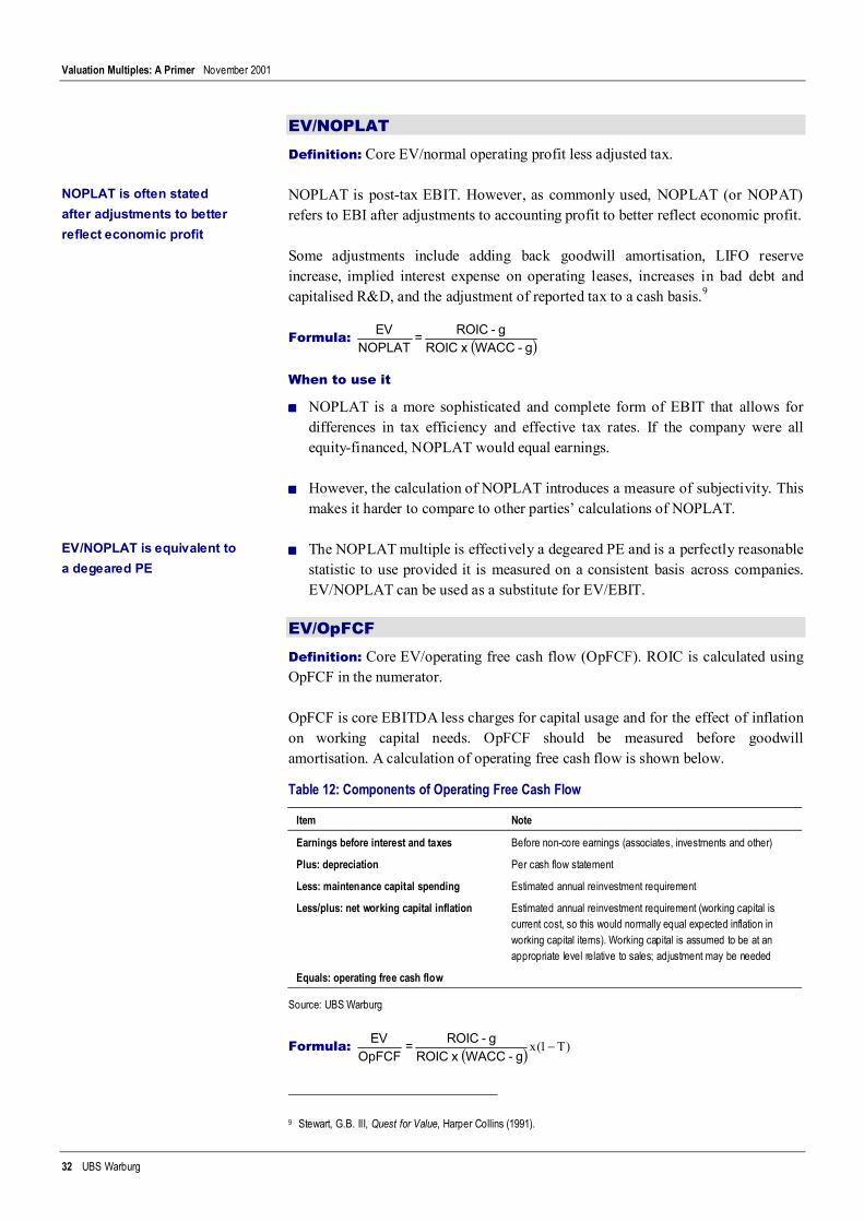
Table 12: Components of Operating Free Cash Flow
Item Note
Earnings before interest and taxes Before non-core earnings (associates, investments and other)
Plus: depreciation Per cash flow statement
Less: maintenance capital spending Estimated annual reinvestment requirement
Less/plus: net working capital inflation Estimated annual reinvestment requirement (working capital iscurrent cost, so this would normally equal expected inflation inworking capital items). Working capital is assumed to be at anappropriate level relative to sales; adjustment may be needed
Equals: operating free cash flow
Source: UBS Warburg
Formula: ( ) )T1(x −g - WACC x ROIC
g - ROIC = OpFCF
EV
9 Stewart, G.B. III, Quest for Value, Harper Collins (1991).
NOPLAT is often statedafter adjustments to betterreflect economic profit
EV/NOPLAT is equivalent toa degeared PE
Valuation Multiples: A Primer November 2001
33 UBS Warburg
When to use it
■■■■ EV/OpFCF is a price to cash flow measure similar to EV/EBIT. OpFCF is not atrue cash flow, however, as it does not include actual capital expenditure orchange in working capital; it is a normalised EBIT or a smoothed cash flow.
■■■■ OpFCF is more comparable than EBITDA and less susceptible to accountingdistortions than EBIT, and is therefore a more suitable basis for valuationmultiples. OpFCF does, however, add another layer of subjectivity via thecalculation of maintenance capital spending and net working capital inflation.
■■■■ EV/OpFCF is preferable to EV/EBITDA for comparing companies within asector, or for comparing companies across sectors or markets where companieshave widely varying degrees of capital intensity.
■■■■ Operating free cash flow is a smoothed measure of free cash flow to the firm, forwhich historical figures can be highly volatile. Because of this, multiples usingOpFCF can be easier to interpret than those using free cash flow.
■■■■ This multiple cannot be used when current cash flow is negative. Usenormalised OpFCF or a forward-priced multiple instead.
EV/Enterprise Free Cash FlowDefinition: Core EV/normalised after-tax core enterprise free cash flow (or FCF,also known as free cash flow to the firm). ROIC is calculated using after-tax FCF inthe numerator.
Formula: ( )g - WACC 1 =
FCFEV
Enterprise Free Cash Flow
Enterprise free cash flow is the cash available to the providers of finance. FCF =debt cash flow + equity cash flow. It may be used:
■■■■ To pay interest or repay debt
■■■■ To build cash balances or other investments
■■■■ To pay dividends or buy back shares
Free cash flow must be after tax and all investment expenditure needed to supportthe future cash flow forecast.
OpFCF is a suitable basisfor valuation than eitherEBITDA or EBIT
Multiples using OpFCFeasier to interpret thanthose using free cash flow
FCF is the cash available toall providers of finance
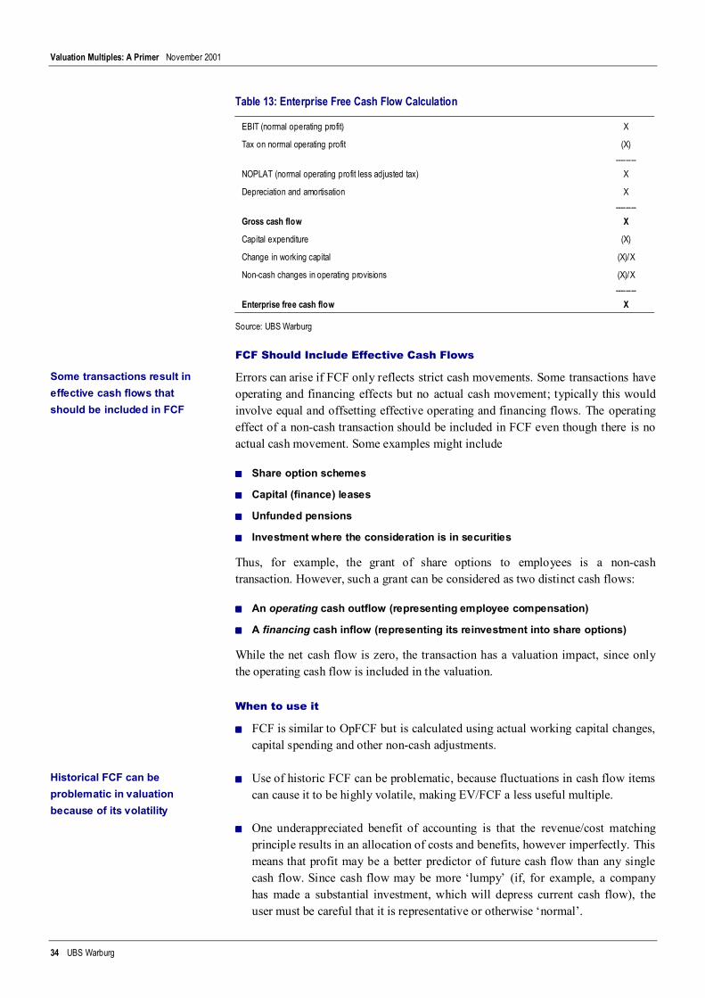
Valuation Multiples: A Primer November 2001
34 UBS Warburg
Table 13: Enterprise Free Cash Flow Calculation
EBIT (normal operating profit) X
Tax on normal operating profit (X)--------
NOPLAT (normal operating profit less adjusted tax) X
Depreciation and amortisation X--------
Gross cash flow X
Capital expenditure (X)
Change in working capital (X)/X
Non-cash changes in operating provisions (X)/X--------
Enterprise free cash flow X
Source: UBS Warburg
FCF Should Include Effective Cash Flows
Errors can arise if FCF only reflects strict cash movements. Some transactions haveoperating and financing effects but no actual cash movement; typically this wouldinvolve equal and offsetting effective operating and financing flows. The operatingeffect of a non-cash transaction should be included in FCF even though there is noactual cash movement. Some examples might include
■■■■ Share option schemes
■■■■ Capital (finance) leases
■■■■ Unfunded pensions
■■■■ Investment where the consideration is in securities
Thus, for example, the grant of share options to employees is a non-cashtransaction. However, such a grant can be considered as two distinct cash flows:
■■■■ An operating cash outflow (representing employee compensation)
■■■■ A financing cash inflow (representing its reinvestment into share options)
While the net cash flow is zero, the transaction has a valuation impact, since onlythe operating cash flow is included in the valuation.
When to use it
■■■■ FCF is similar to OpFCF but is calculated using actual working capital changes,capital spending and other non-cash adjustments.
■■■■ Use of historic FCF can be problematic, because fluctuations in cash flow itemscan cause it to be highly volatile, making EV/FCF a less useful multiple.
■■■■ One underappreciated benefit of accounting is that the revenue/cost matchingprinciple results in an allocation of costs and benefits, however imperfectly. Thismeans that profit may be a better predictor of future cash flow than any singlecash flow. Since cash flow may be more ‘lumpy’ (if, for example, a companyhas made a substantial investment, which will depress current cash flow), theuser must be careful that it is representative or otherwise ‘normal’.
Some transactions result ineffective cash flows thatshould be included in FCF
Historical FCF can beproblematic in valuationbecause of its volatility
Valuation Multiples: A Primer November 2001
35 UBS Warburg
■■■■ Cash flow is better used – in fact is essential – in a discounted cash flowvaluation because multi-period cash flow is used instead of a point estimate. Weprefer the use of a smoothed cash flow figure such as OpFCF, provided theassumptions underlying the calculation are sensible.
EV/Invested CapitalDefinition: core EV/invested capital.
Invested capital, measured from the asset side of the balance sheet, is the sum of nettangible and intangible assets and net working capital. Invested capital excludesnon-core investments and other assets, and to ensure comparability these must alsobe excluded from enterprise value.
Alternative calculations are possible:
■■■■ Total capital employed: Total capital employed is invested capital plusinvestments and associates. Return on total capital employed differs from returnon invested capital in that the numerator for return on total capital employedincludes income from non-core operating investments and other assets. Toensure comparability, enterprise value must also include the value of theseassets.
■■■■ Adjusted capital employed: This is total capital employed adjusted to bringbook capital closer to economic capital. These adjustments (to assets; fromStern, Stewart) include adding back accumulated goodwill amortisation, LIFOreserve and cumulative write-offs of special items, among others.
■■■■ Replacement capital employed: Capital employed at replacement value,intended to better approximate the cost of replacing the capital base at currentprices and therefore the return on assets at market value. This can be roughlyapproximated by adding back accumulated depreciation in addition to makingthe other adjustments noted above.
Formula: g - WACC
g - ROIC or ROIC x g) - (WACC x ROIC
g - ROIC = capital Invested
EV
When to use it
■■■■ The enterprise equivalent of price to book value, EV/invested capital is equal toEV/NOPLAT × ROIC (whereas price to book is equal to PE × ROE).
■■■■ Note that invested capital measures only operating assets whereas net bookvalue includes the value of the firm’s cash holdings. Net income includes returnon cash, but NOPLAT does not. NOPLAT is in this respect a better indication ofcore profitability than net income.
■■■■ This is a useful measure for sectors where tangible assets are key. Because of itsclose linkage to return on capital, it is useful to view this measure together withreturn on capital.
Items included in EV andcapital must be consistent
Invested capital, unlikebook value, excludes non-operating cash
Valuation Multiples: A Primer November 2001
36 UBS Warburg
■■■■ Items included in invested capital or total capital employed must be consistentwith items included in enterprise value.
EV/Capacity MeasureDefinition: Core EV/units of capacity (such as tonnes of cement capacity) oranother revenue-generating unit (such as subscribers).
Formula: ( ) UnitNOPLATx
g - WACC x ROICg - ROIC =
UnitEV
When to use it
■■■■ Enterprise value multiples are often used to compare the implied value ofproductive assets (eg tonnes of cement capacity, fixed telephone lines) to enablecomparison across firms operating within the same industry.
■■■■ This value can be compared to the cost of replacing the asset on a gross basis orafter factoring in depreciation to adjust for the remaining life of the asset in use.
■■■■ A common variant is to look at the implied market value of each revenue-generating unit such as subscribers. Thus the value per, say, customer that themarket ascribes to the firm can then be compared to the amount of revenue orprofit the customer generates.
■■■■ These measures tell us nothing about the relative underlying profitability of theassets nor do they give any other clues about the drivers behind differences invalue. They do not tell us why the (unit of capacity, customer, etc) is valued as itis, nor what the appropriate value should be.
■■■■ Ultimately, the market value of a firm is determined not by the amount ofcapacity it has but by the economic value it creates. There may be wide relativedifferences in EV per widget between companies – and these may be deserved.
■■■■ The way to gauge these differences is to estimate a fair EV per unit multiple bydetermining the sustainable NOPLAT per unit.
■■■■ Consider, for example, a cement firm with a return on capital of 12% growing at3% pa. It if earns US$10 per tonne in operating profit than an investor with arequired return on capital of 10% will be willing to pay up to US$107 per tonneof capacity:
tonne per US$107 US$10 x 10.7 US$10 x .03)-.12(.10
.03-.12 = Tonne
EV ==
EV multiples can be used tocompare crossborderimplied market values ofrevenue-generating units
Differences in per-unitprofitability will determinedifferences in valuation
Valuation Multiples: A Primer November 2001
37 UBS Warburg
Equity MultiplesWhat Are Equity Multiples?An equity multiple, as the name suggests, is the expression of the market value ofequityholders’ stake in an enterprise, relative to a key statistic relating to that value.
As we have noted earlier, the statistic must relate to the value being measured.Since shareholders are subordinate to all other claimants of the cash flow and assetsof a business, any statistic used in an equity multiple must be one that representsresidual profit, cash flow, assets or another residual measure. All senior claims musthave been deducted first.
Equity MultiplesPrice/EarningsDefinition: Current market capitalisation/net income attributable to commonshareholders or alternatively, price per share/attributable earnings per share.
Formula: ( )g -COE x ROEg - ROE
= income Net
cap Market
When to use it
■■■■ The PE ratio is the most commonly used equity multiple (it was first introducedin the 1930s). Data availability is one reason why: earnings, both historical andforecast, are easily available.
■■■■ Earnings are, however, subject to different accounting policies. We recommendusing adjusted earnings in calculating the ratio; UBS Warburg defines ‘adjusted’earnings as earnings before exceptional items and goodwill amortisation.
■■■■ Price to earnings multiples cannot be used when earnings are negative. As analternative, use normalised earnings or calculate a forward-priced multiple (seepage 10).
■■■■ Use this multiple when earnings are representative of future earnings and thetrend in those earnings. For example, if there are significant write-offs in a year,earnings are unlikely to be representative. Use pre-exceptional or pre-extraordinary earnings instead.
■■■■ As far as possible, use for comparisons of companies, sectors and markets thathave similar accounting policies. Alternatives are to adjust earnings to acommon basis across sectors and markets; or to use earnings before the mostmaterial distorting items such as depreciation and goodwill amortisation.
■■■■ Different capital structures will affect multiples because of the gearing effect onearnings; two companies with identical operating profit may have widelydifferent earnings. One alternative approach is to use NOPLAT or tax-adjustedearnings before interest.
Section 5
Equity multiples reflectresidual claims
Use earnings beforeexceptional items andgoodwill amortisation
Gearing will affect the PEmultiple
Valuation Multiples: A Primer November 2001
38 UBS Warburg
■■■■ An important weakness of the PE ratio is that it does not explicitly take intoaccount balance sheet risk (although it is implicitly incorporated into theunderlying cost of equity10).
■■■■ Furthermore, the PE ratio does not explicitly take into account the amount ofinvestment required to support future growth. You can, however, take this intoaccount indirectly (see The Effect of Growth on Value, page 18).
Price/Cash EarningsDefinition: Market capitalisation/net income attributable to common shareholdersplus depreciation, amortisation and changes in non-cash provisions.
Formula: ( ) gsCashearninEarningsx
g -COE x ROE g - ROE =
earnings Cashcap Market
When to use it
■■■■ Cash earnings are usually defined as simply net profit plus depreciation &amortisation. This is a rough and frequently misleading measure of cash flow, asit ignores the many other factors that affect cash flow, including changes in netdebt, changes in working capital and so forth.
■■■■ This problem is magnified when using prospective cash earnings, because of theadditional complications involved in forecasting changes in net debt; theestimated capital structure can have a large impact on forecast earnings.Furthermore, historical cash flow can be a very volatile.
■■■■ As a result, price to cash earnings is difficult to use as a base valuation measure.
■■■■ Price to cash earnings should be used as a supplement to other measures,particularly in conjunction with multiples that are unadjusted for accountingdifferences between comparables, where those differences are material.
Price/Book ValueDefinition: Market capitalisation/book value (alternatively price per share/bookvalue per share).
Formula: g - COEg- ROE or ROE x
g) - (COE x ROEg - ROE =
value Bookcap Market
When to use it
■■■■ Price to book value is a useful measure where tangible assets are the source ofvalue generation. Because of its close linkage to return on equity (price to bookis PE multiplied by ROE), it is useful to view price to book value together withROE.
10 The cost of equity is related to the degree of financial leverage through the equity beta:
( )βdebtβassetED
βassetβequity −+=
Best used as a supplementto other measures
A useful measure wheretangible assets are key
Valuation Multiples: A Primer November 2001
39 UBS Warburg
■■■■ Using this measure with industrial companies requires care because net assetsare based on historical cost book value, an unreliable indicator of economicvalue.
■■■■ Book values are not directly comparable where accounting policies cause themto deviate markedly from economic substance, nor are they directly comparableamong companies with differing accounting policies. For example, book valuewould not be comparable between a company that revalues its assets (permittedunder international accounting standards) and one that does not (revaluation isnot permitted under US GAAP).
■■■■ Ideally, book value should be adjusted for these differences. Some adjustmentsthat might be made include:
— Stripping out revaluation surpluses on the basis that it is more practical thanattempting to revalue all comparables
— Restoring excess depreciation (or deducting inadequate depreciation)
— Restoring accumulated goodwill amortisation and written-off goodwill
— Restoring the LIFO reserve, etc
■■■■ This ratio is most widely used in valuing financials, especially banks, whichsqueeze a small spread from a large base of assets (loans) and multiply thatspread by utilising high levels of leverage (deposits). Return on equity istherefore an important criteria in valuing bank stocks.
Price/Earnings GrowthDefinition: The ‘PEG’ ratio is the prospective PE divided by average forecastearnings growth. It is most widely used to value growth companies where it isassumed that growth opportunities arise from reinvesting at a premium rate ofreturn or from efficiency gains.11
Formula: ( ) g -COE x ROE x g x 100g - ROE =
GrowthPE
When to use it
The PEG is based on the assumption that a PE ratio is positively linearly correlatedto the expected growth rate in earnings, ie PEG is constant. Unfortunately, however,there is no linear relationship between the PE ratio and earnings growth.Nevertheless, PEGs can be used for relative valuation in certain circumstances:
■■■■ Notably, at higher rates of growth PEG ratios are stable and less sensitive tochanges in growth than PE ratios (see chart below), which makes PEG ratiosmore suitable for valuing high-growth companies – for which they are typically
11 For a more detailed discussion of PEG ratios, see our report Price Earnings Growth: A PEG for Your Valuations,November 1997.
Book value should beadjusted to removeaccounting distortions
PEGs most suitable forvaluing high-growthcompanies…
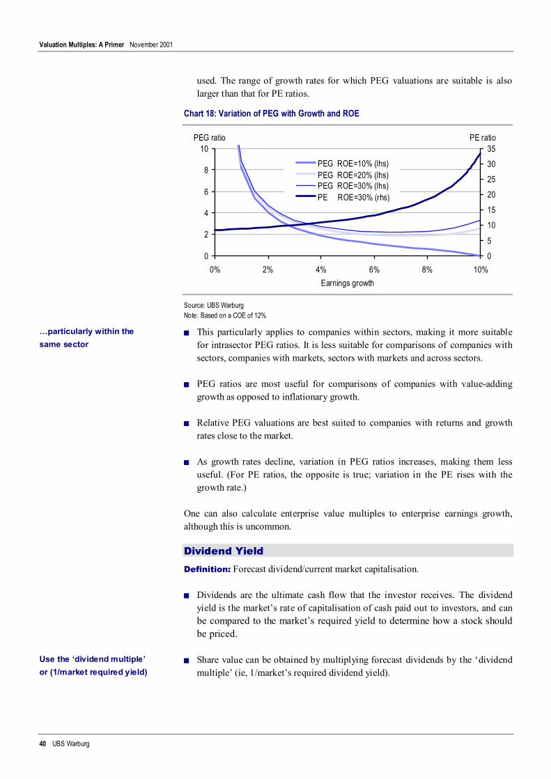
Valuation Multiples: A Primer November 2001
40 UBS Warburg
used. The range of growth rates for which PEG valuations are suitable is alsolarger than that for PE ratios.
Chart 18: Variation of PEG with Growth and ROE
0
2
4
6
8
10
0% 2% 4% 6% 8% 10%Earnings growth
PEG ratio
05
101520253035
PE ratio
PEG ROE=10% (lhs)PEG ROE=20% (lhs)PEG ROE=30% (lhs)PE ROE=30% (rhs)
Source: UBS WarburgNote: Based on a COE of 12%
■■■■ This particularly applies to companies within sectors, making it more suitablefor intrasector PEG ratios. It is less suitable for comparisons of companies withsectors, companies with markets, sectors with markets and across sectors.
■■■■ PEG ratios are most useful for comparisons of companies with value-addinggrowth as opposed to inflationary growth.
■■■■ Relative PEG valuations are best suited to companies with returns and growthrates close to the market.
■■■■ As growth rates decline, variation in PEG ratios increases, making them lessuseful. (For PE ratios, the opposite is true; variation in the PE rises with thegrowth rate.)
One can also calculate enterprise value multiples to enterprise earnings growth,although this is uncommon.
Dividend YieldDefinition: Forecast dividend/current market capitalisation.
■■■■ Dividends are the ultimate cash flow that the investor receives. The dividendyield is the market’s rate of capitalisation of cash paid out to investors, and canbe compared to the market’s required yield to determine how a stock shouldbe priced.
■■■■ Share value can be obtained by multiplying forecast dividends by the ‘dividendmultiple’ (ie, 1/market’s required dividend yield).
…particularly within thesame sector
Use the ‘dividend multiple’or (1/market required yield)

Valuation Multiples: A Primer November 2001
41 UBS Warburg
■■■■ Corporate financiers frequently use market dividend yield as a benchmark forcapitalising dividends in order to estimate the appropriate value for a stock in aninitial public offering.
When to use it
■■■■ Dividends are the ultimate ‘in pocket’ cash flow to investors. They are useful forestimating a floor value for a stock, since both dividends and market yields canbe observed.
■■■■ Keep in mind, however, that actual dividends are subject to corporate dividendpolicy as well as withholding and franking tax policies. Thus nominal dividendyields are not comparable across different tax jurisdictions. When valuing astock, the sustainability of the dividend cash flow must also be considered.
Useful for estimating a floorvalue for a stock
But dividend yields are notcomparable across differenttax regimes
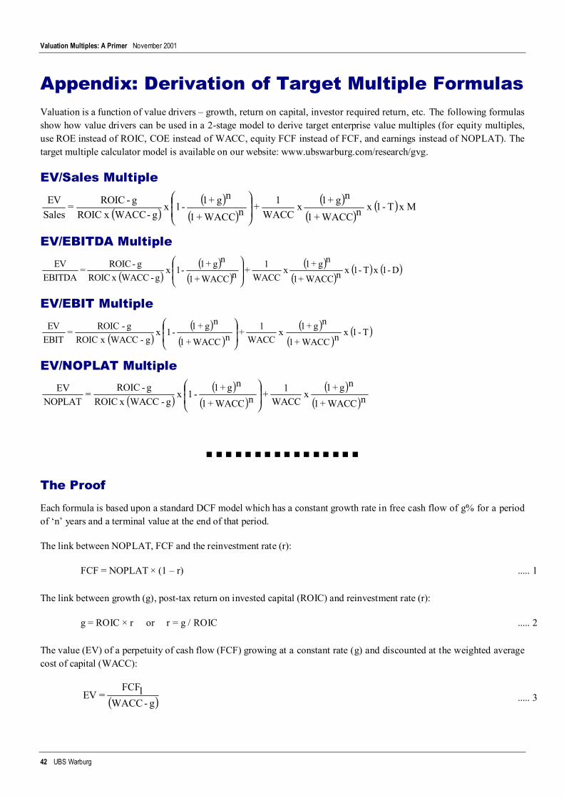
Valuation Multiples: A Primer November 2001
42 UBS Warburg
Appendix: Derivation of Target Multiple FormulasValuation is a function of value drivers – growth, return on capital, investor required return, etc. The following formulasshow how value drivers can be used in a 2-stage model to derive target enterprise value multiples (for equity multiples,use ROE instead of ROIC, COE instead of WACC, equity FCF instead of FCF, and earnings instead of NOPLAT). Thetarget multiple calculator model is available on our website: www.ubswarburg.com/research/gvg.
EV/Sales Multiple
( )( )
( )( )
( )( ) M x T - 1 x n WACC+ 1
ng + 1 x WACC
1 + n WACC+ 1
ng + 1 - 1 x g - WACC x ROIC
g - ROIC = SalesEV
EV/EBITDA Multiple
( )( )
( )( )
( )( ) ( )D - 1 x T - 1 x n WACC+ 1
ng + 1 x WACC
1 + n WACC+ 1
ng + 1 - 1 x g - WACC x ROIC
g - ROIC = EBITDA
EV
EV/EBIT Multiple
( )( )
( )( )
( )( )T - 1 x n WACC+ 1
ng + 1 x WACC
1 + n WACC+ 1
ng + 1 - 1 x g - WACC x ROIC
g - ROIC = EBITEV
EV/NOPLAT Multiple
( )( )
( )( )
( )n WACC+ 1
ng + 1 x
WACC1 + n WACC+ 1
ng + 1 - 1 x
g - WACC x ROICg - ROIC
= NOPLAT
EV
■ ■ ■ ■ ■ ■ ■ ■ ■ ■ ■ ■ ■ ■ ■ ■
The Proof
Each formula is based upon a standard DCF model which has a constant growth rate in free cash flow of g% for a periodof ‘n’ years and a terminal value at the end of that period.
The link between NOPLAT, FCF and the reinvestment rate (r):
FCF = NOPLAT × (1 – r) ..... 1
The link between growth (g), post-tax return on invested capital (ROIC) and reinvestment rate (r):
g = ROIC × r or r = g / ROIC ..... 2
The value (EV) of a perpetuity of cash flow (FCF) growing at a constant rate (g) and discounted at the weighted averagecost of capital (WACC):
( )g - WACC1FCF
= EV ..... 3

Valuation Multiples: A Primer November 2001
43 UBS Warburg
Formula 3 above can be modified to apply to a growing annuity of cash flows which stops after n years:
( )( )
( )
n WACC+ 1
ng + 1 - 1 x
g - WACC1FCF
= EV ..... 4
Substituting equations 1 and 2 into 3 gives:
( )g - WACCROIC
g - 1 x 1NOPLAT
= EV
..... 5
and rearranging:
( )( )g - WACC x ROIC
g - ROIC x 1NOPLAT = EV ..... 6
In calculating a terminal value at the end of the growth period, it is assumed that ROIC equals WACC (ie conditions ofzero value-adding growth). Therefore equation 6 becomes:
WACC 1NOPLAT
= EV ..... 7
Formulae 1 and 2 can also be substituted into equation 4. Following rearrangement this becomes:
( )( )
( )( )
n
n1
WACC+ 1g + 1 - 1 x
g - WACC x ROICg - ROIC x NOPLAT = EV ..... 8
Putting it Together
Equation 8 represents the value of cash flows in the growth period. Equation 7 can be used to value subsequent cashflows, although NOPLAT1 needs to be replaced by NOPLAT(n+1) and this ‘terminal value’ must be discounted to apresent value. The overall value then becomes:
( )( )
( )( )
( )( )n
n1
n
n1
WACC+ 11
x WACC
g + 1 x NOPLAT +
WACC+ 1g + 1
- 1 x g - WACC x ROIC
g - ROIC x NOPLAT = EV
..... 9
Dividing by NOPLAT1 gives the formula for the EV/NOPLAT multiple:
( )( )
( )( )
( )( )n
n
n
n
1 WACC+ 1
g + 1 x
WACC1
+ WACC+ 1
g + 1 - 1 x
g - WACC x ROICg - ROIC
= NOPLAT
EV
..... 10
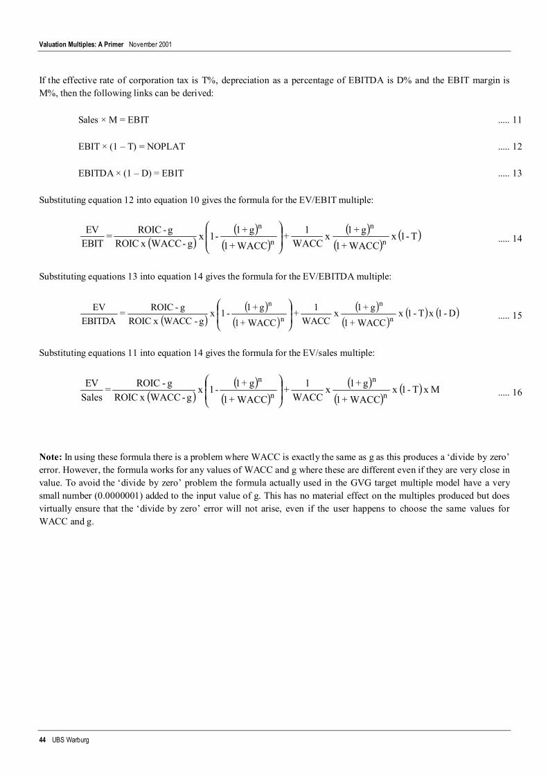
Valuation Multiples: A Primer November 2001
44 UBS Warburg
If the effective rate of corporation tax is T%, depreciation as a percentage of EBITDA is D% and the EBIT margin isM%, then the following links can be derived:
Sales × M = EBIT ..... 11
EBIT × (1 – T) = NOPLAT ..... 12
EBITDA × (1 – D) = EBIT ..... 13
Substituting equation 12 into equation 10 gives the formula for the EV/EBIT multiple:
( )( )
( )( )
( )( )T - 1 x
WACC+ 1g + 1 x
WACC1 +
WACC+ 1g + 1 - 1 x
g - WACC x ROICg - ROIC =
EBITEV
n
n
n
n
..... 14
Substituting equations 13 into equation 14 gives the formula for the EV/EBITDA multiple:
( )( )
( )( )
( )( ) ( )D - 1 x T - 1 x
WACC+ 1g + 1 x
WACC1 +
WACC+ 1g + 1 - 1 x
g - WACC x ROICg - ROIC =
EBITDAEV
n
n
n
n
..... 15
Substituting equations 11 into equation 14 gives the formula for the EV/sales multiple:
( )( )
( )( )
( )( ) M x T - 1 x
WACC+ 1g + 1 x
WACC1 +
WACC+ 1g + 1 - 1 x
g - WACC x ROICg - ROIC =
SalesEV
n
n
n
n
..... 16
Note: In using these formula there is a problem where WACC is exactly the same as g as this produces a ‘divide by zero’error. However, the formula works for any values of WACC and g where these are different even if they are very close invalue. To avoid the ‘divide by zero’ problem the formula actually used in the GVG target multiple model have a verysmall number (0.0000001) added to the input value of g. This has no material effect on the multiples produced but doesvirtually ensure that the ‘divide by zero’ error will not arise, even if the user happens to choose the same values forWACC and g.

Valuation Multiples: A Primer November 2001
45 UBS Warburg

Valuation Multiples: A Primer November 2001
46 UBS Warburg
This report was produced by:UBS Warburg
+44-20-7567 8000
Head office:1 Finsbury AvenueLondonEC2M 2PPUK
UBS Warburg, 1 Finsbury Avenue, London, EC2M 2PP, UK Phone: +44-20-7567 8000
This report has been prepared by the division, group, subsidiary or affiliate of UBS AG (“UBS”) identified herein. In certain countries UBS AG is referred to as UBS SA, which is atranslation of UBS AG, its registered legal name. UBS Warburg is a business group of UBS AG. This report is for distribution only under such circumstances as may bepermitted by applicable law, including the following:This report has no regard to the specific investment objectives, financial situation or particular needs of any specific recipient. The report is published solely for informationalpurposes and is not to be construed as a solicitation or an offer to buy or sell any securities or related financial instruments. The securities described herein may not be eligiblefor sale in all jurisdictions or to certain categories of investors. The report is based on information obtained from sources believed to be reliable but is not guaranteed as beingaccurate, nor is it a complete statement or summary of the securities, markets or developments referred to in the report. The report should not be regarded by recipients as asubstitute for the exercise of their own judgement. Any opinions expressed in this report are subject to change without notice and UBS is not under any obligation to update orkeep current the information contained herein. UBS and/or its directors, officers and employees may have or have had interests or long or short positions in, and may at any timemake purchases and/or sales as principal or agent, or UBS may act or have acted as market-maker in the relevant securities or related financial instruments discussed in thisreport. Furthermore, UBS may have or have had a relationship with or may provide or has provided corporate finance, capital markets and/or other financial services to therelevant companies. Employees of UBS may serve or have served as officers or directors of the relevant companies. UBS may rely on information barriers, such as “ChineseWalls,” to control the flow of information contained in one or more areas within UBS, into other areas, units, divisions, groups, or affiliates of UBS.Options, derivative products and futures are not suitable for all investors, and trading in these instruments is considered risky. Past performance is not necessarily indicative offuture results. Foreign currency rates of exchange may adversely affect the value, price or income of any security or related instrument mentioned in this report. Clients wishingto effect transactions should contact their local sales representative. UBS accepts no liability whatsoever for any loss or damage of any kind arising out of the use of all or anypart of this report. Additional information will be made available upon request.EEA: This report has been issued by UBS Warburg Ltd., regulated in the UK by the Securities and Futures Authority. In the UK this report is for distribution to persons who arenot UK private customers. Customers should approach the analyst(s) named on the cover regarding the contents of this report. For investment advice, trade execution or anyother queries, customers should contact their London representative. Switzerland: This report is being distributed in Switzerland by UBS AG. Italy: Should persons receivingthis research in Italy require additional information or wish to effect transactions in the relevant securities, they should contact either Giubergia UBS Warburg SIM SpA, anassociate of UBS SA, in Milan or UBS Warburg (Italia) SIM SpA, a subsidiary of UBS SA, in Milan or its London or Lugano Branch. South Africa: UBS Warburg Securities(South Africa) (Pty) Ltd. (incorporating J.D. Anderson & Co.) is a member of the JSE Securities Exchange SA. United States: This report is being distributed to US persons byeither UBS Warburg LLC or by UBS PaineWebber Inc., subsidiaries of UBS AG; or (ii) by a division, group, subsidiary or affiliate of UBS AG, that is not registered as a USbroker-dealer (a “non-US affiliate”), to major US institutional investors only. UBS Warburg LLC or UBS PaineWebber Inc. accepts responsibility for the content of a reportprepared by another non-US affiliate when distributed to US persons by UBS Warburg LLC or UBS PaineWebber Inc. All transactions by a US person in the securitiesmentioned in this report must be effected through UBS Warburg LLC or UBS PaineWebber Inc., and not through a non-US affiliate. Canada: This report is being distributed byUBS Bunting Warburg Inc., a subsidiary of UBS AG and a member of the principal Canadian stock exchanges & CIPF. A statement of its financial condition and a list of itsdirectors and senior officers will be provided upon request. Singapore: This report is being distributed in Singapore by UBS Warburg Pte. Ltd. Hong Kong: This report is beingdistributed in Hong Kong to investors who fall within section 3(1) of the Securities Ordinance (Cap 333) by UBS Warburg Asia Limited. Japan: This report is being distributed inJapan by UBS Warburg (Japan) Limited to institutional investors only. Australia: This report is being distributed in Australia by UBS Warburg Australia Limited in relation to fixedincome securities, and UBS Warburg Australia Equities Limited in relation to equity securities. New Zealand: This report is being distributed in New Zealand by UBS WarburgNew Zealand Ltd in relation to fixed income securities and UBS Warburg New Zealand Equities Ltd in relation to equity securities.© 2001. All rights reserved. No part of this report may be reproduced or distributed in any manner without the written permission of UBS. UBS specifically prohibits the re-distribution of this report, via the Internet or otherwise, and accepts no liability whatsoever for the actions of third parties in this respect.
VAD0215C