VALLIAMMAI ENGINEERING COLLEGE

SRM Nagar, Kattankulathur – 603 203

DEPARTMENT OF

MECHANICAL ENGINEERING

QUESTION BANK

VI SEMESTER

ME 6603 Finite Element Analysis

Regulation – 2013

Academic Year 2017 – 18

Prepared by

Mr. S.Senthil Babu, Assistant Professor/MECHANICAL ENGINEERING Mr. R. Ramkumar, Assistant Professor/MECHANICAL ENGINEERING

Mr.J.Arunraj, Assistant Professor/MECHANICAL ENGINEERING

VALLIAMMAI ENGINEERING COLLEGE

SRM Nagar, Kattankulathur – 603 203.

DEPARTMENT OF MECHANICAL ENGINEERING

QUESTION BANK

UNIT I: INTRODUCTION

Historical Background – Mathematical Modeling of field problems in Engineering – Governing

Equations – Discrete and continuous models – Boundary, Initial and Eigen Value problems–

Weighted Residual Methods – Variational Formulation of Boundary Value Problems – Ritz

Technique – Basic concepts of the Finite Element Method.

PART A

1 llustrate the methods generally associated with the finite element

analysis. BT2 Understanding

2 If a displacement field in x direction is given by u=2x2+4y

2+6xy.

Determine the strain in x direction BT3 Applying

3 Point out any four advantages of finite element method BT3 Applying

4 Explain polynomial type interpolation function mostly preferred BT4 Analyzing

5 State the advantages of Rayleigh Ritz method. BT2 Understanding

6 Compare the Ritz technique with the nodal approximation method. BT4 Analyzing

7 How to develop the equilibrium equation for a finite element? BT6 Creating

8 Summarize discretization. BT2 Understanding

9 List the various method of solving boundary value problems. BT1 Remembering

10 Formulate the boundary conditions of a cantilever beam AB of span L

fixed at A and free at B subjected to a uniformly distributed load of P

throughout the span

BT6 Creating

11 Name the weighted residual methods BT1 Remembering

12 How will you identify types of Eigen Value Problems? BT1 Remembering

13 Explain weak formulation of FEA BT4 Analyzing

14 Distinguish between Error and Residual BT2 Understanding

15 Discuss Ritz method. BT5 Evaluating

16 How will you develop total potential energy of a structural system? BT6 Creating

17 Explain the principle of minimum potential energy. BT4 Analyzing

18 Differentiate between initial value problem and boundary value

problem. BT2 Understanding

19 List out the advantages of finite element method over other numerical

analysis method. BT1 Remembering

20 List the various weighted residual methods BT1 Remembering

PART B

1 Using any one of the weighted residue method, find the displacement of

given governing equation 𝑑

𝑑𝑥 𝑥

𝑑𝑢

𝑑𝑥 -

2

𝑥2 = 0, 1 < 𝑥 < 2 BT3 Applying

2 Using collocation method, find the solution of given governing equation 𝑑2Φ

𝑑𝑋2 + Φ + X = 0, 0 ≤ X ≤ 1 subject to the boundary conditions

Φ 0 = Φ 1 = 0. Use X=14 and 1 2 as the collocation points.

BT3 Applying

3 A uniform rod subjected to a uniform axial load is illustrated in figure,

the deformation of the bar is governed by the differential equation given

below. Determine the displacement by applying Weighted Residual

Method (WRM).

BT3 Applying

4 Describe the step by step procedure of solving FEA. BT4 Analyzing

5 Explain the process of discretization of a structure in finite element

method in detail, with suitable illustration for each aspect being and

discussed.

BT1 Remembering

6 (i)Enumerate the advantages & disadvantages of FEM. BT3 Applying

(ii) Discuss the factors to be considered in discretization of a domain. BT2 Understanding

7 Find the approximate deflection of a simply supported beam under a

uniformly distributed load ‘P’ throughout its span. By applying Galerkin

and Least Square Residual Method

BT3 Applying

8 Solve the differential equation for a physical problem expressed as

d2y/dx

2 + 100 = 0, 0≤x≤10

with boundary conditions as y(0)=0 and y(10)=0 using (i) Point

collocation method (ii) Sub domain collocation method (iii) Least

square method and (iv) Galerkin method

BT2 Understanding

9 A physical phenomenon is governed by the differential equation the

boundary conditions are given by assuming a trial solution

w(x)=a0+a1x+a2x2+a3x

3

determine using Galerkin method.The variation of ,’w’, with respect to x

BT5 Evaluating

10 (i) Find the solution of the initial value problem.

𝑦′ + 𝑦 = 0 ; 𝑦 3 = 2 BT6 Creating

(ii) Find a solution of the initial value problem 02

2

2

ydx

dy

dx

yd,

boundary conditions y(0) = 2, 𝑦′ (0)=5.

BT6 Creating

11 The following differential equation is available for a physical

phenomenon, d2y/dx

2 – 10x

2 =5, 0≤x≤1 with boundary conditions as y

(0) = 0 and y (1) = 0. Find an approximate solution of the above

differential equation by using Galerkin’s method of weighted residuals

and also compare with exact solution.

BT4 Analyzing

12 Solve the ordinary differential equation d2y/dx

2 + 10 x

2 = 0, 0≤x≤1 with

boundary conditions as y (0) = 0 and y (1) = 0 using the Galerkin’s

method with the trial function No(x) = 0; N1(x) = x (1-x2).

BT3 Applying

13 Solve the differential equation for a physical problem expressed as

d2y/dx

2 + 50 = 0, 0≤x≤10 with boundary conditions as y (0) = 0 and y

(10) = 0 using the trial function y = a1x (10-x) find the value of the

parameters a1 by the following methods listed below.

(i) Point collocation method (ii) Sub domain collocation method

(iii) Least squares method and (iv) Galerkin method

BT3 Applying

14 Find the solution of the boundary value problem 𝑦′′ + 4𝑦 = 0 with

y 𝜋

8 =0, y

𝜋

6

BT6 Creating

PART C (15 Marks)

1 Find the eigen value and eigen function of 𝑦′′ − 4𝜆𝑦′+4𝜆2𝑦 = 0; with

the boundary conditions are 𝑦′ 1 = 0, 𝑦 2 + 2𝑦′ 2 = 0. BT6 Creating

2 A beam AB of span ‘l’ simply supported at the ends and carrying a

concentrated load ‘W’ at the centre ‘C’ as shown in figure .Determine

the deflection at the mid span by using Rayleigh-Ritz method and

compare with exact solution.

BT6 Creating

3 Determine the expression for deflection and bending moment in a

simply supported beam subjected to uniformly distributed load over

entire span. Find the deflection and moment at mid span and compare

with exact solution Rayleigh-Ritz method. Use

BT5 Evaluating

4 Calculate the value of central deflection in the figure below by assuming

Y = a sin πx/L the beam is uniform throughout and carries and central

point load P.

BT3 Applying

. UNIT 2 ONE-DIMENSIONAL PROBLEMS

One Dimensional Second Order Equations – Discretization – Element types- Linear and Higher order

Elements – Derivation of Shape functions and Stiffness matrices and force vectors- Assembly of

Matrices - Solution of problems from solid mechanics and heat transfer. Longitudinal vibration

frequencies and mode shapes. Fourth Order Beam Equation –Transverse deflections and Natural

frequencies of beams

PART A

1 Identify the types of problems consider as one dimensional problem. BT1 Remembering

2 Define shape function. BT1 Remembering

3 Illustrate shape function of a two node line element BT3 Applying

4 List out the stiffness matrix properties. BT1 Remembering

5 Describe the characteristics of shape functions BT2 Understanding

6 Differentiate global and local coordinate. BT2 Understanding

7 Express the element stiffness matrix of a truss element BT2 Understanding

8 Illustrate a typical truss element shown local global transformation BT3 Applying

9 Define natural coordinate system BT1 Remembering

10 Give the shape function equation for a 1D quadratic bar element. BT2 Understanding

11 List the types of dynamic analysis problems BT1 Remembering

12 Define mode superposition technique. BT1 Remembering

13 Express the mass matrix for a 1D linear bar element. BT2 Understanding

14 List out the expression of governing equation for free axial vibration of

rod and transverse vibration of beam. BT1 Remembering

15 Determine the element mass matrix for one-dimensional dynamic

structural analysis problems. Assume the two-node, linear element. BT4 Analyzing

16 Write down the Governing equation and for 1D longitudinal vibration of

a bar fixed at one end and create the boundary conditions BT6 Creating

17 Explain the transverse vibration. BT4 Analyzing

18 Deduce the stiffness matrix for a 1D two noded linear element. BT5 Evaluating

19 Show that in what way the global stiffness matrix differs from element stiffness matrix? BT3 Applying

20 Illustrate the expression of longitudinal vibration of the bar element. BT3 Applying

PART B

1 Formulate the shape function for One-Dimensional Quadratic bar

element. BT6 Creating

2 A steel bar of length 800mm is subjected to an axial load of 3kN as

shown in fig. estimate the nodal displacement of the bar and load

vectors

BT2 Understanding

3 For the bar element as shown in the figure. Calculate the nodal

displacements and elemental stresses

BT3 Applying

4 Determine the Eigen values for the stepped bar shown in figure

BT5 Evaluating

5 Consider a bar as shown in figure an axial load of 200kN is applied at a

point P. Take A1=2400 mm2 , E1=70x10

9 N/mm

2 A2=600 mm

2 and E2 =

200x109 N/mm

2 . Calculate the following (i) the nodal displacement at

point,P (ii) Stress in each element (iii) Reaction force.

BT4 Analyzing

6 For a tapered bar of uniform thickness t=10mm as shown in figure.

Predict the displacements at the nodes by forming into two element

model. The bar has a mass density ρ = 7800 kg/m3, the young’s

modulus E = 2x105 MN/m

2. In addition to self-weight, the bar is

subjected to a point load P= 1 kN at its centre.Also determine the

reaction forces at the support.

BT2 Understanding

7 Consider a bar as shown in fig Young’s Modulus E=2 x 105 N/mm

2 A1=

2 cm2;A2 = 1cm

2 and force of 100N. Calculate the nodal displacement.

BT3 Applying

8 A metallic fin 20 mm wide and 4 mm thick is attached to a furnace

whose wall temperature is 180 °C. The length of the fin is 120 mm. if

the thermal conductivity of the material of the fin is 350 W/m °C and

convection coefficient is 9 W/m2 °C, determine the temperature

distribution assuming that the tip of the fin is open to the atmosphere

and that the ambient temperature is 25 °C.

BT5 Evaluating

9 Calculate the temperature distribution in the stainless steel fin shown in

the figure. The region can be discretized in three elements of equal sizes

BT2 Understanding

10 Determine the maximum deflection for the beam loaded as shown in

Fig. Young's modulus 200 GPa and density 0.78×104kg/m3. The beam

is of ‘T’ cross section shown in Fig.

BT4 Analyzing

11 Examine the natural frequencies of transverse vibrations of the cantilever beam shown in figure by applying one 1D beam element.

BT1 Remembering

12 A two noded truss element is shown in figure. The nodal displacements

are u1=5mm and u2= 8mm. calculate the displacement at x=L/4, L/3 and

L/2

BT3 Applying

13 For the two bar truss shown in the fig, Estimate the displacements of

node 1 and the stress in element 1-3.Take E=70GPa A=200 mm2

BT4 Analyzing

14 Calculate the displacements and slopes at the nodes for the beam shown in

figure.Find the moment at the midpoint of element 1

BT3 Applying

PART C

1 Develop the Shape function, Stiffness matrix and force vector for

one dimensional linear element. BT6 Creating

2 Consider the bar shown in figure axial force P = 30kN is applied as

shown. Determine the nodal displacement, stresses in each element and

reaction forces

BT5 Evaluating

3 For the beam and loading as shown in figure. Calculate the slopes at

nodes 2 and 3 and the vertical deflection at the mid-point of the

distributed load. Take E=200 GPa and I=4x10-6

m4

BT3 Applying

4 Calculate the force in the members of the truss as shown in fig. Take

E=200 GPa

BT3 Applying

UNIT 3 TWO DIMENSIONAL SCALAR VARIABLE PROBLEMS

Second Order 2D Equations involving Scalar Variable Functions – Variational formulation –Finite

Element formulation – Triangular elements – Shape functions and element matrices and vectors.

Application to Field Problems - Thermal problems – Torsion of Non circular shafts –Quadrilateral

elements – Higher Order Elements.

PART A

1 Show the displacement function equation for CST element. BT3 Applying

2 How will you modify a three-dimensional problem to a Two-

dimensional problem? BT6 Creating

3 List out the application of two-dimensional problems. BT1 Remembering

4 Express the shape functions associated with the three noded linear

triangular element and plot the variation of the same. BT2 Understanding

5 Define two-dimensional scalar variable problem BT1 Remembering

6 How do you define two dimensional elements? BT1 Remembering

7 Explain QST (Quadratic strain Triangle) element. BT4 Analyzing

8 Relate path line with streamline. BT3 Applying

9 Formulate the (B) matrix for CST element. BT6 Creating

10 Express the interpolation function of a field variable for three-node

triangular element BT2 Understanding

11 List out the CST and LST elements. BT1 Remembering

12 Illustrate the shape function of a CST element. BT3 Applying

13 Define LST element. BT1 Remembering

14 Express the nodal displacement equation for a two dimensional

triangular elasticity element BT2 Understanding

15 Show the transformation for mapping x-coordinate system into a natural

coordinate system for a linear spar element and for a quadratic spar

element. BT3 Applying

16 What do you understand by area coordinates? BT2 Understanding

17 Define Isoparametric elements with suitable examples BT1 Remembering

18 Explain shape function of four node quadrilateral elements. BT4 Analyzing

19 Explain geometric Isotropy. BT5 Evaluating

20 Write the Lagrange shape functions for a 1D, 2noded elements. BT5 Evaluating

PART B

1 Develop the element strain displacement matrix and element stiffness

matrix of a CST element BT6 Creating

2 Determine the shape functions for a constant strain triangular (CST)

element BT5 Evaluating

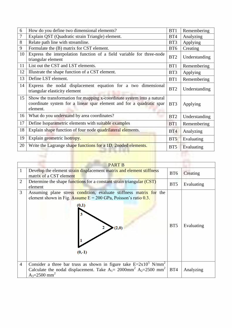
3 Assuming plane stress condition, evaluate stiffness matrix for the

element shown in Fig. Assume E = 200 GPa, Poisson’s ratio 0.3.

BT5 Evaluating

4 Consider a three bar truss as shown in figure take E=2x105 N/mm

2

Calculate the nodal displacement. Take A1= 2000mm2 A2=2500 mm

2

A3=2500 mm2

BT4 Analyzing

5 Determine the stiffness matrix for the CST element shown in figure. The

coordinates are given in mm. Assume plane strain conditions.

E=210GPa v=0.25 and t=10 mm

BT5 Evaluating

6 Derive the expression for shape function for heat transfer in 2D element. BT2 Understanding

7 Calculate the value of pressure at the point A which is inside the 3

noded triangular element as shown in fig. The nodal values are Φ1 = 40

MPa, Φ2 = 34 MPa and Φ3 = 46 MPa. point A is located at (2, 1.5).

Assume the pressure is linearly varying in the element. Also determine

the location of 42 MPa contour line.

BT3 Applying

8 For a 4-noded rectangular element shown in fig. Infer the temperature at

the point (2.5, 2.5). The nodal values of the temperatures are T1= 100°C,

T2= 60°C and T3= 50°C and T4= 90°C. Also determine the 80°C

isotherm.

BT4 Analyzing

9 Calculate the element stiffness matrix and temperature force vector for

the plane stress element shown in fig. The element experiences a 20ºC

increase in temperature. Assume α= 6x10-6

C. Take E=2x105 N/mm

2,

BT3 Applying

v= 0.25, t= 5mm.

10 For a 4-noded rectangular element shown in fig. Estimate the

temperature point (7,4). The nodal values of the temperatures are T1 =

42˚C, T2 = 54˚C and T3 = 56˚Cand T4 = 46˚C. Also determine 3 point on

the 50˚C contour line.

BT2 Understanding

11 The figure below shows a shaft having rectangular cross section with 8

cm x 4 cm sides. The material has shear modulus 80 x 105

N/mm2

. Shaft

length is 100 cm. the shaft is fixed at one end and subjected to torque T

at the other end. Determine the total angle of twist if the applied torque

is 10 x 103 N-cm

BT5 Evaluating

12 Determine the pressure at the location (7, 4) in a rectangular plate with

the data shown in Fig and also draw 50 MPa contour line.

BT4 Analyzing

13 Develop the shape function derivation for a two-dimensional quadratic

element BT6 Creating

14 Estimate the stiffness matrix for the triangular element with the (x,y)

coordinates of the nodes are (0,-4), (8,0) and (0,4) at nodes i, j, k. Assume

plane stress condition E= 200 GPa, Poisson’s ratio = 0.35

BT5 Evaluating

PART C

1 The x,y coordinates of nodes i,j and k of a triangular element are given

by (0,0) (3,0) and (1.5,4) mm respectively. Evaluate the shape functions

N1,N2 and N3 at an interior point P(2,2.5)mm of the element. Evaluate

the strain displacement relation matrix B for the above same triangular

element and explain how stiffness matrix is obtained assuming scalar

variable problem.

BT5 Evaluating

2 For the triangular element shown in the figure determine the strain-

displacement matrix [B] and constitutive matrix [D]. Assume plane

stress conditions. Take µ=0.3 , E=30 x 106

N/m2 and thickness t= 0.1 m.

And also calculate the element stiffness matrix for the triangular

element

BT4 Analyzing

3 Determine the temperature distribution in the rectangular fin shown in

Fig. The upper half can be meshed taking into account symmetry using

triangular elements.

BT4 Analyzing

4 For the square shaft of cross section 1 cm × 1 cm as shown in Fig. It

was decided to determine the stress distribution using FEM by solving

for the stress function values. Considering geometric and boundary

condition symmetry 1/8th

of the cross section was modeled using two

triangular elements and one bilinear rectangular element as shown. The

element matrices are given below. Carry out the assembly and solve for

the unknown stress function values.

For triangular K = 1 2 1 −1 0

−1 2 −10 −1 1

r = 29.129.129.1

BT3 Applying

For rectangle K = 1 6

4121

1412

2141

1214

r =

6.43

6.43

6.43

6.43

UNIT 4 TWO DIMENSIONAL VECTOR VARIABLE PROBLEMS

Equations of elasticity – Plane stress, plane strain and axisymmetric problems – Body forces and

temperature effects – Stress calculations - Plate and shell elements

PART A

1 Illustrate the Stress-Strain relationship matrix for an axisymmetric

triangular element. BT3 Applying

2 Classify the types of shell element. BT4 Analyzing

3 Define 2D vector variable problems BT1 Remembering

4 List out the various elasticity equations. BT1 Remembering

5 Define plane stress and plane strain. BT1 Remembering

6 Discuss ‘Principal stresses”. BT2 Understanding

7 Discuss the difference between the use of linear triangular elements and

bilinear rectangular elements for a 2D domain. BT2 Understanding

8 Define axisymmetric solid. BT1 Remembering

9 Distinguish between plane stress, plane strain and axisymmetric analysis in solid mechanics.

BT2 Understanding

10 Show the machine component related with axisymmetric concept. BT3 Applying

11 Discuss axisymmetric formulation. BT2 Understanding

12 Develop the Shape functions for axisymmetric triangular elements BT6 Creating

13 Explain about finite element modeling for axisymmetric solid. BT4 Analyzing

14 Develop the Strain-Displacement matrix for axisymmetric solid BT6 Creating

15 Show the Stress-Strain displacement matrix for axisymmetric solid BT3 Applying

16 Deduce the Stiffness matrix for axisymmetric solid BT5 Evaluating

17 Assess the requried conditions for a problem assumed to be

axisymmetric.. BT5 Evaluating

18 State whether plane stress or plane strain elements can be used to model

the following structures. Explain your answer.

A wall subjected to wind load

A wrench subjected to a force in the plane of the wrench.

BT4 Analyzing

19 Define a plane strain with suitable example. BT1 Remembering

20 Define a plane stress problem with a suitable example. BT1 Remembering

PART B

1 Determine the stiffness matrix for the axisymmetric element shown in

figure. Take E=2.1 x 105 N/mm

2, v=0.25 The coordinates are in mm.

BT3 Applying

2 Develop shape function for axisymmetric triangular elements BT6 Creating

3 Triangular element are used for the stress analysis of plate subjected to

inplane loads. The (x,y) coordinates of nodes i, j, and k of an element

are given by (2,3), (4,1), and (4,5) mm respectively. The nodal

displacement are given as :

u1=2.0 mm, u2=0.5 mm, u3= 3.0 mm v1=1.0 mm, v2= 0.0 mm, v3= 0.5

mm Examine element stress. Let E=160GPa, poisson's ratio = 0.25 and

thickness of the element t=10 mm

BT1 Remembering

4 The nodal coordinates for an axisymmetric triangular element are given

in figure. Evaluate the strain-displacement matrix

BT5 Evaluating

5 The nodal coordinates for an axisymmetric triangular element shown in

fig are givenbelow. Examine the strain-displacement matrix for that

element

BT1 Remembering

6 Calculate the element stiffness matrix for the axisymmetric triangular

element shown in fig. The element experiences a 15ºC increase in

temperature. The coordinate are in mm. Take α=10x10-6

/ºC, E=2x105

N/mm2, v=0.25.

BT3 Applying

7 The nodal coordinates for an axisymmetric triangular element shown in

fig are given below. Evaluate the strain-displacement matrix for that

element

BT4 Analyzing

8 Calculate the element strains for an axisymmetric triangular element

shown in fig the nodal displacement are. u1= 0.001, u2 = 0.002, u3 = -

0.003, w1 = 0.002, w2 = 0.001 and w3 = 0.004 all dimensions are in mm.

BT3 Applying

9 Estimate the global stiffness matrix for the plate shown in fig. Taking

two triangular elements. Assume plane stress conditions

BT2 Understanding

10 Explain the classification of the shell elements and also brief the

assumptions used in Finite element Analysis of Shell element. BT4 Analyzing

11 (i) Explain the assumptions made in the thin plate and thick plate theory BT4 Analyzing

(ii) List the advantages of using shell elements. BT1 Remembering

12 Evaluate the Stress-Strain relationship matrix for axisymmetric

triangular element BT5 Evaluating

13 Develop Strain-Displacement matrix for axisymmetric triangular

element BT6 Creating

14 Derive the Finite element equation for triangular plate bending element

with 9 degrees of freedom. BT4 Analyzing

PART C

1 Develop the four basic sets of elasticity equation BT6 Creating

2 A long hollow cylinder of inside diameter 100mm and outside diameter

120mm isfirmly fitted in a hole of another rigid cylinder over its full

length as shown in fig.The cylinder is then subjected to an internal

pressure of 2 MPa. By using two element on the 10mm length shown

calculate the displacements at the inner radius tame E = 210 GPa. μ =

0.3

BT3 Applying

3 Triangular element are used for the stress analysis of plate subjected to

inplane loads. The (x,y) coordinates of nodes 1, 2, and 3 of an element

are given by (5,5), (25,5), and (15,15) mm respectively. The nodal

displacement are given as : u1=0.005 mm, u2=0.002 mm, u3= 0.0 mm,

u4=0.0 mm, u5= 0.005 mm, u6= 0.0 mm.Evaluate element stress. Let

E= 200 GPa, poisson's ratio = 0.3 and use unit thickness of the element

BT5 Evaluating

4 For an axisymmetric triangular elements as shown in fig. Evaluate the

stiffness matrix. Take modulus of elasticity E = 210 GPa. Poisson’s

ratio = 0.25. the coordinates are given in millimeters

BT5 Evaluating

UNIT 5 ISOPARAMETRIC FORMULATION

Equations of elasticity – Plane stress, plane strain and axisymmetric problems – Body forces and temperature

effects – Stress calculations - Plate and shell elements.

PART A

1 Illustrate the purpose of Isoparameteric element. BT4 Analyzing

2 Differentiate between Isoparametric, super parametric and sub-

parametric elements. BT1 Remembering

3 Define Isoparametric formulation BT5 Evaluating

4 Explain the Jacobian transformation BT2 Understanding

5 Give the shape functions for a four-noded linear quadrilateral element in

natural coordinates. BT2

Understanding

6 Describe the Jacobian of transformation for two-noded Isoparametric

element. BT1 Remembering

7 List out the advantages of Gauss quadrature numerical integration for

Isoparametric element BT1 Remembering

8 Define Isoparametric element BT2 Understanding

9 Discuss about Numerical integration BT2 Understanding

10 Discuss about Gauss-quadrature method. BT4 Analyzing

11 Differentiate between implicitly and explicitly methods of numerical

integration BT4

Analyzing

12 Differentiate between geometric and material non-linearity. BT1 Remembering

13 List out the significance of Jacobian transformation BT1 Remembering

14 Define Isoparametric element with suitable examples. BT6 Creating

15 Develop Stress- displacement matrix for Four noded quadrilateral

element using natural coordinates. BT6

Creating

16 Develop Stiffness matrix for Isoparametric quadrilateral element BT1 Remembering

17 Define Newton cotes quadrature method BT2 Understanding

18 Distinguish between trapezoidal rule and Simpson’s rule BT2 Understanding

19 Distinguish between trapezoidal rule and Gauss quadrature. BT5 Evaluating

20 Explain the transformation for mapping x-coordinate system into a

natural coordinate system for a linear spar element and for a quadratic

spar element

BT4 Analyzing

PART B

1 Examine the shape function for 4 noded rectangular element by using

natural coordinate system. BT1 Remembering

2 Evaluate the Jacobian matrix for the isoparametric quadrilateral element

shown in the figure

BT3 Applying

3 Develop the shape function for 4 noded isoparametric quadrilateral element BT6 Creating

4 Develop the strain displacement matrix, stress-strain matrix and

stiffness matrix for an isoparametric quadrilateral element BT6 Creating

5 Evaluate the Jacobian matrix at the local coordinates ε=η= 0.5 for

the linear quadrilateral element with its global coordinates as shown in

fig. Also evaluate the strain-displacement matrix

BT5 Evaluating

6 For the four noded quadrilateral element shown in fig analysis the

Jacobian and evaluate its value at the point (1/2, 1/2)

BT4 Analyzing

7 Calculate the Cartesian coordinates of the point P which has local BT3 Applying

coordinates ε = 0.8 and η = 0.6 as shown in figure

8

Evaluate

1

1

24 dxxx by applying 3 point Gaussian quadrature. BT5 Evaluating

9 Evaluate dxe x

1

1

by applying 3 point Gaussian quadrature. BT5 Evaluating

10 Evaluate the integral, I =

1

12

dxx

Cos

by applying 3 point Gaussian

quadrature and compare with exact solution.

BT4 Analyzing

11 For a four noded rectangular element shown in fig. Estimate the

following a. Jacobian matrix b. Strain-Displacement matrix c. Element strain

and d. Element stress

BT2 Understanding

12 For the element shown in the figure. Calculate the Jacobian matrix.

BT3 Applying

13 Consider the isoparametric quadrilateral element with nodes 1 to 4 at

(5,5), (11,7),(12,15), and (4,10) respectively. Estimate the jacobian

matrix and its determinant at the element centroid

BT2 Understanding

14 Tabulate the element characteristics of a four node quadrilateral element BT1 Remembering

PART C (15 MARKS)

1 Evaluate the integral by two point Gaussian Quadrature, I= BT3 Applying

dxdyyxyx )432( 2

1

1

1

1

2

.Gauss points are +0.57735 and -0.57735

each of weight 1.0000

2 i) Derive the shape function for all the corner nodes of a nine noded

quadrilateral element.

ii) Using Gauss quadrature evaluate the following integral using 1,2 and

3 point integration.

𝐒𝐢𝐧 𝐒

𝐒 (𝟏−𝐒𝟐)

𝟏

−𝟏 𝐝𝐬

BT6 Creating

3 For the four noded element shown in Fig,

(i) determine the Jacobian and evaluate its value at the point 1 3, 1 3

(ii) Using energy approach derive the stiffness matrix for a 1D linear

isoparametric element.

BT5 Evaluating

4 For the isoparametric quadrilateral element shown in figure, the

Cartesian coordinates of point ‘P’, are (6,4). The loads 10 kN and 12 kN

are acting in x and y direction on that point P. Evaluate the nodal forces.

BT4 Analyzing