1

Validation of numerical prediction of dynamic derivatives: two test cases

B. Mialon*1, Alex. Khrabrov2, Saloua Ben Khelil3, Andreas Huebner4, Andrea Da Ronch5, Ken Badcock5, Luca Cavagna6, Peter Eliasson6, Mengmeng Zhang7, Sergio Ricci8, Jean-Christophe Jouhaud9, Gilbert Rogé10, Stephan Hitzel11, Martin Lahuta12 (1) ONERA, 5 Boulevard Paul Painlevé, F-59045, Lille, France (2) TsAGI, Zhukovsky, Russia, 140180 (3) ONERA, 8 rue des Vertugadins, 92190, Meudon, France (4) DLR, Braunschweig, Germany (5) University of Liverpool, Liverpool, UK L69 3BX, United Kingdom (6) Swedish Defence Research Agency (FOI), SE-164 90 Stockholm, Sweden (7) Royal Institute of Technology (KTH), Stockholm, Sweden (8) Politecnico di Milano, Milano, 20156, Italy (9) CERFACS, Toulouse, France (10) Dassault-Aviation, Saint-Cloud, France (11) EADS MAS, Manching, Germany (12) VZLU, Prague, Czech Republic

Abstract

The dynamic derivatives are widely used in linear aerodynamic models in order to determine the flying qualities of an aircraft: the ability to predict them reliably, quickly and sufficiently early in the design process is vital in order to avoid late and costly component redesigns. This paper describes experimental and computational research dealing with the determination of dynamic derivatives carried out within the FP6 European project SimSAC. Numerical and experimental results are compared for two aircraft configurations: a generic civil transport aircraft, wing-fuselage-tail configuration called the DLR-F12 and a generic Transonic CRuiser (TCR), which is a canard configuration. Static and dynamic wind tunnel tests have been carried out for both configurations and are briefly described within this paper. The data generated for both the DLR-F12 and TCR configurations includes force and pressure coefficients obtained during small amplitude pitch, roll and yaw oscillations whilst the data for the TCR configuration also includes large amplitude oscillations, in order to investigate the dynamic effects on nonlinear aerodynamic characteristics. In addition, dynamic derivatives havebeen determined for both configurations with a large panel of tools, from linear aerodynamic (Vortex Lattice Methods) to CFD (unsteady Reynolds-Averaged Navier-Stokes solvers). This work confirms that an increase in fidelity level enables the dynamic derivatives to be calculated more accurately. Linear aerodynamics (VLM) tools are shown to give satisfactory results but are very sensitive to the geometry/mesh input data. Although all the quasi-steady CFD approaches give comparable results (robustness) for steady dynamic derivatives, they do not allow the prediction of unsteady components for the dynamic derivatives (angular derivatives w.r.t. time): this can be done with either a fully unsteady approach (with a time-marching scheme) or with Frequency Domain solvers, both of which provide comparable results for the DLR-F12 test case. As far as the canard configuration is concerned; strong limitations for the linear aerodynamic tools are observed. A key aspect of this work are the acceleration techniques developed for CFD methods, which allow the computational time to be dramatically reduced while providing comparable results.

* Corresponding author. Tel.: +33 3 20 49 69 07; fax: +33 3 20 49 69 53. E-mail address: Bruno.Mialon@onera.fr

2

Key Words Dynamic Derivatives – Acceleration Techniques – Conceptual Design – Wind Tunnel – Computational Fluid

Dynamics

Content

Validation of numerical prediction of dynamic derivatives: two test cases..............................................................1 Abstract ....................................................................................................................................................................1 Key Words................................................................................................................................................................2 Content .....................................................................................................................................................................2 Nomenclature ...........................................................................................................................................................2 I. Introduction ......................................................................................................................................................3 II. Computational tools ...................................................................................................................................4

A. CEASIOM..................................................................................................................................................4 B. Linear tools ................................................................................................................................................6 C. CFD tools ...................................................................................................................................................6

III. The DLR-F12 test case...............................................................................................................................7 A. Experimental data base ..............................................................................................................................8 B. Selection of conditions for computations...................................................................................................9 C. Numerical approaches and tools ................................................................................................................9 D. Analysis of results – Aerodynamic Coefficients/Derivatives...................................................................11 E. Pitch Motion.............................................................................................................................................12 F. Roll Motion ..............................................................................................................................................17 G. Yaw Motion .............................................................................................................................................17

IV. The Transcruiser test case: TCR ..............................................................................................................18 A. From virtual shape to wind-tunnel model ................................................................................................18 B. Wind tunnel tests......................................................................................................................................19 C. Benchmark comparisons with CFD results ..............................................................................................25

V. Conclusion ...............................................................................................................................................28 Acknowledgments ..................................................................................................................................................28 References ..............................................................................................................................................................28

Nomenclature H = altitude MD = design cruise Mach number S = reference area b = wing span c = mean aerodynamic chord xCG = position of the center of gravity from the fuselage apex V∞ = upstream flow velocity Re = Reynolds number α = angle of attack αA = amplitude = angle of sideslip φc = canard deflection CL = lift force coefficient (aerodynamic fixed frame) CN = normal force coefficient (model fixed frame) CY = side force coefficient (model fixed frame) Cl = rolling moment coefficient (model fixed frame) Cm = pitching moment coefficient (aerodynamic/model fixed frame) Cn = yawing moment coefficient (model fixed frame) f = frequency

3

p, q, r = roll, pitch, yaw rate

k = reduced frequency ( Vfck / )

I. Introduction HE design process of a new aircraft classically begins with a sizing of the main components using very simple models or rules. At this early stage, the aerodynamic characteristics are in general estimated from

tabulated data and the flying qualities from simple stability and control criteria applied to the longitudinal short period or the lateral Dutch roll mode, which are established using analytical formula. Once a first viable configuration has been created, a process of refinement is undertaken through the use of higher fidelity models. For the aerodynamics, this can consist of linear tools such as Vortex Lattice Methods, because their use is relatively straightforward and does not require the time consuming generation of smooth CAD shapes and the volumic grids required by CFD. The next step in the design process is typically the wind tunnel testing of the proposed configuration, possibly in addition to CFD computations. The flight control system (FCS) design arrives late in this process, and generally uses a model which can be created using multiple sources of aerodynamic data. This type of model is generally based on the conventional aerodynamic derivatives approach, introduced by Bryan1 one century ago, with a linear relationship between the forces,moments and flight states. For instance, the model for an increment in lift and pitching moment can be expressed as follows:

CiV

lqCi

V

lCiCi q

where i denoted L (lift) or m (pitching moment) (1)

(A) (B) (C) The first part of the equation, (A), represents the purely static effects. The term denoted (B) is related to the

steady dynamic effects while the term (C) describes the unsteady dynamic effects. Similar equations can be written for the lateral coefficients undergoing pitch and yaw rotary motions. In this model, nonlinear, high-order, frequency-dependent, or time-dependent terms are assumed to be negligible along with other simplifying assumptions. However, this linear model is considered suitable for the determination of aircraft flying qualities in most representative aerodynamic conditions.

During an harmonic motion in pitch, of amplitude A and frequency f, one can write:

)2sin( fA (2)

)2cos(2 ffq A

Eq. (1) becomes:

)2cos()(2

)2sin( fCiCiV

flfCiCi qAA

(3)

where Ci represents the in-phase component and CiCiq represents the out-of-phase component of Ci .

The dynamic derivatives can be computed considering the first Fourier coefficients of the time history of Ci . An alternative way to derive the derivatives is the linear regression technique2.

The experimental determination of dynamic derivatives requires specific rigs to simulate harmonic motions

with small amplitudes in wind tunnels. The most common rigs perform pitch, roll or yaw oscillations, which allow steady dynamic derivatives to be determined. The unsteady dynamic derivatives with respect to pitch ( ) can be determined directly through harmonic plunge motions at fixed angle of attack (q=0). The derivatives with

respect to yaw angle ( ) can similarly be deduced experimentally e.g. from several kinematic combinations

using rotary balances3. Most of the existing dynamic rigs are implemented in low speed wind tunnels and usually require specific models (light weight, constraints on first structural eigenfrequency, etc.). These experimental activities can also be time-consuming and expensive. In addition, the experimental results can suffer from the effects of model support interaction, wall interference and imperfect aerodynamic similitude: corrections exist for some of these, but in general not for all.

The dynamic derivatives can also be obtained through numerical simulation. Pure rotary motions can be

simulated through quasi steady approaches, with linear tools like vortex-lattice methods (VLM) as well as with

T

4

CFD tools solving Euler or Navier-Stokes equations; the rotation of the computational domain results from the composition of a translation (mean flow velocity) and an additional rotation velocity. This allows steady dynamic derivatives to be computed. The determination of unsteady dynamic derivatives requires time-marching solvers, which compute the time history of aerodynamic forces during harmonic variations of the state variable of interest (pitch angle, sideslip, etc.). From this, the unsteady dynamic derivatives can then be derived using for example, a Fourier transformation of the aerodynamic forces. The unsteady computations remain time-consuming but acceleration methods exist, which take advantage of the periodic nature of the motion to decrease the computational cost of fully unsteady simulations4.

This paper deals with the benchmarking of dynamic derivatives prediction tools. For this purpose, two test

cases have been considered: - the DLR-F12 test case, a generic civil wing fuselage tail configuration; - the Transonic CRuiser (TCR), a generic transonic passenger aircraft specifically designed within the

SimSAC project. Experimental data bases have been generated for both configurations and been used within this work to

benchmark a range of computational tools employed in virtual aircraft designto calculate dynamic derivatives, from linear methods through to full CFD. CFD results obtained using acceleration techniques are also developed and considered. The next section gives a brief overview of computational tools employed, with subsequent sections providing the results for both the DLR-F12 and TCR test cases respectfully. All the results presented in this paper have been obtained in the framework of the SimSAC project, a FP6 European Project*.

II. Computational tools This section provides a brief overview of each of the tools used to within this paper, separated into three

sections. The first one deals with CEASIOM, the framework tool developed in the SimSAC project and which includes aerodynamic codes evoked in sections III and IV. The second one deals with linear tools (the so-called “TIER1” category in the SimSAC project) and the third one with CFD tools (the so-called “TIER1+” and “TIER2” category in the SimSAC project).

A. CEASIOM CEASIOM5 is a framework tool that integrates discipline-specific tools such as: CAD & mesh generation,

CFD and stability & control analysis ,all designed for the purpose of aircraft conceptual design. Figure 1 presents an overview of the CEASIOM software, showing aspects of its functionality, process and dataflow. * http://www.simsacdesign.eu

5

Figure 1. SimSAC generated CEASIOM Software (with reference?) Significant features developed and integrated in CEASIOM as modules are the following: 1) Geometry module Geo-SUMO A customized geometry construction system coupled to surface and volume grid generators; Port to CAD via

IGES. 2) Aerodynamic module AMB-CFD A replacement of and complement to current handbook aerodynamic methods with new adaptable fidelity

modules referred to as Tier I (a.), Tier I + (b.), and Tier II (c.): a. Steady and unsteady TORNADO vortex-lattice code (VLM) for low-speed aerodynamics and aero-

elasticity b. Inviscid Edge CFD code for high-speed aerodynamics and aero-elasticity c. RANS (Reynolds Averaged Navier-Stokes) flow simulator for high-fidelity analysis of extreme flight

conditions 3) Stability and Control module S&C A simulation and dynamic stability and control analyzer and flying-quality assessor. Six Degrees of Freedom

test flight simulation, performance prediction, including human pilot model, Stability Augmentation System (SAS), and a LQR based flight control system (FCS) package are among the major functionalities of this module.

4) Aero-elastic module NeoCASS Quasi-analytical structural sizing, FE model generation, linear aeroelastic analysis (static aeroelasticity,

flutter assessment) and structural optimization. Low fidelity panel methods usually adopted; interface with Edge flow solver for medium fidelity analysis.

5) Flight Control System design module FCSDT A designer toolkit for flight control-law formulation, simulation and technical decision support, permitting

flight control system design philosophy and architecture to be coupled in early in the conceptual design phase. 6) Decision Support System module DSS An explicit DSS functionality, including issues such as fault tolerance and failure tree analysis. In this paper, dynamic derivatives obtained with TORNADO, Inviscid Edge and NeoCASS are presented, in

addition to results obtained with alternative tools from outside of the CEASIOM environment.

6

B. Linear tools The linear tools considered within SimSAC are vortex and doublet lattice methods and panel methods. The

meshes used were constructed from the three-view drawing of the configurations along with the camber distribution of the wing and horizontal tail plane. In addition to the Athena Vortex Lattice program (AVL), developed at MIT6,7, and the TAGAZOU software, developed at ONERA for inhouse usa only, the following software has been employed:

1. SMARTCAD8,9

SMARTCAD is the numerical kernel within NeoCASS devoted to aeroelastic analysis. Different kinds of results can be generated using the classical linear approach: trim solution for the free flying aircraft, aerodynamic derivative corrections for the aeroelastic effects, flutter assessment and structural optimization to satisfy aeroelastic and structural constraints. A linear stick model is usually adopted to represent structural deformability. Two low-fidelity aerodynamic methods are available in SMARTCAD, depending on whether steady or unsteady analysis is to be carried out:

• irrotational, isoentropic and inviscid flow via a Vortex Lattice Method (VLM) with camber contribution when the airfoil description is provided;

• Doublet Lattice Method (DLM) for the prediction of the generalized forces due to harmonic motion in the subsonic regime.

Both methods are based on potential flow theory leading, under the hypothesis of irrotational, isoentropic and inviscid flow, to a Laplace’s equation respectively for the linearized velocity or acceleration potential.

2. Native UNST10,11

The UNST code has been developed at TsAGI and employs a classical VLM formulation. The aircraft surface is approximated using horse-shoe vortices and the circulation of each vortex is time dependent in order to take into account unsteady motion. and The code allows the full out-of-phase dynamic derivatives (i.e. including

and derivatives) to be determined.

3. TORNADO/CEASIOM12

The TORNADO code was originally developed at KTH and within the SimSAC project, has been substantially upgraded. One of the tasks required was to integrate the unsteady part of the native UNST code (from TsAGI) within TORNADO. The updated code is called TORNADO/CEASIOM, and is fully embedded within the CEASIOM framework.

C. CFD tools The tools used within this work are Euler and RANS solvers, employing different numerical approaches.

These tools enable the steady and/or the unsteady dynamic derivatives to be computed, depending on the assumptions and numerical features used: all the non linear tools allow the computations of steady dynamic derivatives, through the so-called “quasi-steady” approache: the addition of a rotary motion to the geometry leads to a modified steady state problem for the flow solution. The computation of the unsteady dynamic derivatives requires numerical methods with a time-marching scheme.

1. TAU

TAU is the unstructured code developed at DLR13. In this “Linearized Frequency Domain Method”, the input consists of an initial steady flow field on the mesh and a specification of a harmonic motion of the geometry (amplitude and frequency). The motion of the geometry can be simulated through an ALE formulation. The output consists of complex Fourier coefficients at each point of the mesh which describe the amplitude and phase of the resulting flow perturbation. These coefficients can then be integrated over the surface of the geometry in order to obtain amplitude and phase information for the force coefficients.

2. EUGENIE

This code is developed by Dassault-Aviation14,15 and is used for aerodynamic as well as aeroelastic simulations, solving the RANS equations in the time domain on unstructured grids. As with the TAU code, a

7

Linearized Frequency Domain Method has been introduced in order to efficiently approximate the effect of small, periodically unsteady perturbations of the configuration geometry on the associated flow field. The geometry motion can be considered through an ALE formulation or a transpiration technique.

3. elsA

The elsA software is the multi-block structured solver developed at ONERA, which is applied to a wide variety of aerodynamics flows16. As far as dynamic derivatives predictions are concerned, the user can compute steady dynamic derivatives using an ALE formulation applied to a finite-difference approach, and unsteady dynamic derivatives using ALE with a time-marching scheme.

4. EDGE+ROM EDGE is a Navier-Stokes solver originating from FOI17,18 and solves the Euler and RANS equations on

unstructured grids. The Euler version of the code has been embedded in the CEASIOM framework. In order to determine the dynamic derivatives, a Reduced Order Model process has been implemented19,

which consists of a linear transfer matrix in the frequency domain taken from numerical experiments in the time domain. A step input is given in terms of boundary motion (rigid or deformable), then the responses are computed (body forces or generalized forces) and Fast Fourier Transformed (FFT). The ROM is constructed considering the ratio of output over input for a range of frequency values of interest.

Once the ROM is available, dynamic aerodynamic derivatives for different values of reduced frequency can be calculated and used for flight mechanic applications20. Following the classical approach in linear aeroelasticity, quasi-steady corrections due to structural deformability can also be taken into account. This allows the aero-elastic effects on the maneuver and handling qualities to be considered from the very start of the design process.

5. PMB

The PMB (Parallel Multi-Block) solver has been developed at the University of Liverpool. The Euler and RANS equations are discretised on curvilinear multi-block body conforming grids using a cell-centred finite volume method which converts the partial differential equations (PDE’s) into a set of ordinary differential equations (ODE’s). The equations are solved on block structured grids using an implicit solver. A wide variety of unsteady flow problems, including aeroelasticity, cavity flows, aerospike flows, delta wing aerodynamics, rotorcraft problems and transonic buffet have been studied by means of this code. The main features of the CFD solver are detailed in Badcock et al.21. The PMB code also allows unsteady (time-domain) aerodynamic solutions to be computed. This can be applied to the determination of dynamic derivatives. In order to save computational time, and to take advantage of the periodic nature of the motion, a Harmonic Balance method has recently been implemented in the PMB solver4,22 and some results from the application of this method are presented in this paper.

6. NSMB23

The Navier Stokes Multi Block solver (NSMB) was developed from 1992 until 2003 in a consortium which included Airbus France and SAAB Military Aircraft. Since 2004 NSMB has been further developed in a new consortium lead by CFS Engineering and composed of RUAG Aviation (Emmen), Astrium Space Technologies (France), EPFL (Lausanne), EHTZ (Zürich), IMFT (Toulouse), IMFS (Strasbourg), the Technical University of München and the University of the Army in München. NSMB employs the cell-centred Finite Volume method using multi block structured grids to discretize the Navier Stokes equations. Various space discretization schemes are available to approximate the inviscid fluxes. The time integration is carried out using either the explicit Runge Kutta scheme or the semi-implicit LU-SGS scheme. Various convergence acceleration methods are available, among them local time-stepping, preconditioning, grid sequencing and multigrid. Well tested turbulence models in NSMB include the Spalart-Allmaras 1 equation model and different variants of the k-ω models including the Menter Shear Stress variant.

III. The DLR-F12 test case The DLR-F12 configuration is a conventional wing-fuselage-tail configuration for civil passenger transport.

It was selected in the SimSAC project as the reference benchmark configuration for comparison of the dynamic derivatives prediction methods..

8

A. Experimental data base The DLR-F12 model used was constructed specifically for the dynamic tests, and as such, must meet different design criteria to conventional wind tunnel models. The mass of a dynamic wind-tunnel model as well as the moments of inertia must be as low as possible to achieve a favorable ratio between the aerodynamic forces of interest and the additional inertial forces. In addition, the elastic deformation has to be as small as possible. Furthermore, the first Eigenfrequency of the model should be one order of magnitude above the excitation frequency, i.e. at least 15 Hz, in order to avoid the excitation of the model's higher harmonics. The best material to meet all these requirements proves to be carbon fibre reinforced plastic (CFRP). Using a CFRP-Sandwich structure, the resulting DLR-F12 model had a mass of 12 kg and was manufactured by the DLR plastics workshop in Braunschweig. In order to evaluate the influence of individual components of the tested aircraft configurations, such as winglets, vertical or horizontal stabilizers, nacelles, on the dynamic derivatives, the models are designed in a modular way. The DLR-F12 model does not only allow the measurement of unsteady forces and moments but also unsteady pressure distributions using pressure taps at specific chordwise stations on the wing and horizontal and vertical stabilizers. In the SimSAC project, static and dynamic force measurements as well as steady and unsteady pressure distribution measurements in three sections distributed on the wing, the horizontal and the vertical tail planes, have been performed on the DLR-F12 configuration in the 3m Low Speed Wind Tunnel of the foundation German-Dutch Wind Tunnels (DNW-NWB) in Braunschweig, Germany. For the experimental determination of the dynamic wind tunnel data a new combined motion test capability was developed by DNW and DLR as an improved successor to the previous test set-ups, using a unique six degree-of-freedom test rig called ‘Model Positioning Mechanism’ (MPM) as shown in Figure 2

The static tests included - and -sweeps and in the dynamic tests the model performed forced sinusoidal oscillations in roll, pitch and yaw. Two different configurations which comprise a fuselage-wing geometry with and without a vertical and a horizontal tail plane were also considered. Details of the experimental work can be found in 24.

Figure 2. DLR-F12 model on the MPM. Figure 3. Axis-system for force

coefficients. The calculation of the derivatives is based on the assumption that the wind tunnel model is ideally rigid. It is

also assumed that the aerodynamic forces and moments are linear functions of the model position and the angular speed. As a consequence, the derivatives with respect to drag can be calculated but don’t meet the assumptions. The dynamic derivatives derived from the wind tunnel test are summarized in Table 1.

Table 1. Dynamic Derivatives derived from the DNW-NWB wind tunnel.

Steady Unsteady Dynamic Derivatives Force Moments Force Moments

9

Pitch motion (q) CLCLq CmCmq

Roll motion (p) CYp

Clp

Cnp

Yaw motion (r) CYCYr ClClr

CnCnr

B. Selection of conditions for computations Some static and forced-motion test conditions have been selected from the experimental data base for

comparison with computation results. The objective of the selection is to establish the ability as well as the productivity of different tools to predict stability and control derivatives. The rationale behind this selection was to include, as far as possible, non linear behaviors as well as dependency on parameters (frequency, amplitude). The speed for all computations is V=70m/s, which corresponds to a Reynolds number based on reference chord lμ of Re1.2 millions. Although the transition was triggered in the experiment (fuselage nose, wing, empennage), all computations considered fully turbulent flows. Static test conditions

Numerical simulations were first conducted on static test conditions in order to check the ability of tools to match forces and pressures. Angles of attack from -5 to 8.2° for longitudinal flows (=0º) and sideslips from -5 to +5° at =6.15°, were considered. Forced-motion test conditions

The numerical computations on the forced-motion cases concerned a single motion around each axis of the model-axis system (Fig. 3), with a frequency of 3 Hz and amplitudes of approximately 4.5°:

Table 2. Selection of forced-motion tests conditions.

Motion Amplitude Frequency f0 Reduced Frequency*

Mean angle of attack

Mean sideslip

Required approach

q 4.52° 3Hz 0,068 0=0º 0=0º Quasi-steady (q) q 4.52° 3Hz 0,068 0=0º 0=0º Unsteady (q + ) p 4.86° 3Hz 0,068 0=6º 0=0º Quasi-steady (p) r 4.32° 3Hz 0,068 0=6º 0=0º Quasi-steady (r)

The roll and yaw motions required computation using the complete configurations whilst the pitch motion

was computed considering the half configuration only. One can note that FOI computed the three motion cases

using an unsteady (time-dependent) approach, so for the yaw motion “r”, the derivatives with respect to are

also included in their results.

C. Numerical approaches and tools Table 3 indicates the tools that have been used by each partner.

Table 3. Tools employed by each SimSAC partner. Linear Simulations

Partner Tool Type of theory/equations ONERA TAGAZOU Vortex Lattice Method TSAGI Time Dependent VLM Vortex Lattice Method VZLU AVL Vortex Lattice Method

Reduced Order Models Partner CFD code Type of approach

DASSAULT EUGENIE Linearized frequency Euler code DLR TAU Linear Frequency Domain solver

Non Linear Simulations

10

Partner CFD code Type of mesh CERFACS elsA Structured DASSAULT EUGENIE Unstructured (tetrahedra) DLR TAU Unstructured/hybrid EADS MAS TAU Unstructured/hybrid FOI EDGE Unstructured/hybrid LIVERPOOL PMB Structured ONERA elsA Structured

1. Structured and Unstructured Meshes

The CFD computations were conducted on the basis of two sets of meshes generated by CERFACS/ONERA (structured) and DLR (unstructured). For both approaches, meshes suited for Euler and RANS equations were created, for the half model as well as the complete wing-fuselage-tail configurations. In addition, a specific mesh suited for wall functions was derived from the structured RANS mesh. The geometric and aerodynamic quality of these grids was carefully checked and compared, with a specific attention to the first cell size (y+), before being delivered to the partners (Figure 4). The next table summarizes the size of each mesh:

Table 4. Size of the CFD meshes

Half configuration Full config. Half configuration Full config. Structured Unstructured

Euler 1.7 106 cells 3.4 106 cells 1.92 106 nodes 3.84 106 nodes RANS 11.1 106 cells 22.2 106 cells 8.6 106 nodes 17.2 106 nodes RANS+wall functions 8.9 106 cells 17.8 106 cells - -

The grids used for “linear methods” were produced by each individual SimSAC partner, based on a three-view drawing of the aircraft. The grid densities are the following:

Table 5. Size of the meshes used with linear tools VLM Number of vortices for the

geometric model ONERA 1920 TsAGI 1 442 TsAGI 2 1348 VZLU 1560

Figure 4. Comparison of structured and unstructured grids

2. Computational Efficiency It is difficult to compare the computational efficiency of different tools used by different partners on different

computers, given the distributed nature of the work. However, one can consider some rough estimates based on the available information and giving the approximate time required for each fidelity level. The figures indicated in the next table are expressed in hours and correspond to a moderately parallelized solver (typically 12 processors).

11

Table 6. Typical elapsed time for computations of the DLR-F12 configuration Configuration Fidelity Steady Quasi-steady Unsteady Frequency Domain

Solver Full VLM 0,02 h 0,04 h

Euler 0,5 h 1 h 30 h 1 h Half (unstructured solver) RANS 10 h 20 h 300 h

The order of magnitude for one run of VLM tools is the minute. A quasi steady computation requires

approximately the time for two steady computations, while an unsteady computation requires 15 to 20 times the computational cost of a quasi steady computation. The Frequency Domain Solver is in the class of a quasi-steady computation.

D. Results for steady computations The computed aerodynamic coefficients are compared with the experimental data in Figure 5 (coefficientvalue versus angle of attack, aerodynamic axis system) and figure 6 (coefficient value versus sideslip, model axis system). The lift coefficient is well predicted by the CFD tools with a lift overestimation by Euler methods for the highest angles of attack. A shift in the pitching moment of about 0.03 exists between experimental and computational data and is likely to come from the model support effect (ventral sting), not taken into account in the computations. As far as the VLM tools are concerned, the discrepancy of the results is large, possibly arising from differences in the geometries and/or meshes employed.

[°]

CM

-5 -4 -3 -2 -1 0 1 2 3 4 5 6 7 8 9 10

-0.30

-0.20

-0.10

0.00

0.10

0.20

0.30

[°]

CL

-6 -5 -4 -3 -2 -1 0 1 2 3 4 5 6 7 8 9 10

-0.6

-0.4

-0.2

0.0

0.2

0.4

0.6

0.8

1.0

TN 2320, rn 1002, FWVH, U=70 m/sDLR, EulerDLR, NSONERA, NS Spalart AllmarasCERFACS, NS Spalart Allmaras with Wall LawDASSAULT, EulerDASSAULT, NS, k-epsEADS, EULEREADS, NS SAEEADS, NS WILCOXFOI, EulerFOI, NSVZLUUniv. Liverpool, EulerUniv. Liverpool, NSTsAGIAleniaONERA - TAGAZOU

Figure 5. Lift and Pitching Moment coefficients versus Angle of Attack

The lateral coefficients shown in Figure 6 are relatively well predicted using all the methods employed.

12

/ °

Cn

-5 -4 -3 -2 -1 0 1 2 3 4 5

-0.04

-0.02

0.00

0.02

0.04

/ °

Cl

-5 -4 -3 -2 -1 0 1 2 3 4 5

-0.04

-0.02

0.00

0.02

0.04

/ °

CY

-5 -4 -3 -2 -1 0 1 2 3 4 5-0.10

-0.08

-0.06

-0.04

-0.02

0.00

0.02

0.04

0.06

0.08

0.10

TN2320, rn 1006, FWVH, = 6° CYDLR, EulerDLR, NSONERA, NS Spalart AllmarasCERFACS, NS Spalart Allmaras with Wall LawDASSAULT, EulerDASSAULT, NS k-epsEADS, EULEREADS, NS SAEEADS, NS WILCOXFOI, NSTsAGI, VLMVZLU, VLMAleniaONERA, VLM

Figure 6. Side force, Rolling and Yawing Moment Coefficients versus Sideslip Angle

When comparing Euler and Navier-Stokes results, it can be seen that the viscous effects are moderate for this

configuration. Although not shown here, the calculated pressure coefficient distributions in all three sections are in an excellent agreement with the experimental data.

E. Pitch Motion 1. Quasi-steady computations The steady dynamic derivatives are plotted in Figure 7 for the lift and pitching moment coefficients. The experimental data exhibit a non significant dependency on the angle of attack. The plots include results obtained with linear inviscid tools as well as Euler and Navier-Stokes solvers. The experimental data includes the contribution for derivatives and the scattering for the static derivatives establishes in the region of 15/20% of the absolute values of the q derivatives, which is relatively small if one considers the large differences in the flow models. The viscous effects are slightly higher for the pitching moment derivative (10% of the absolute value) than for the lift (5%).

13

/ °C

Lq

-1 0 1 2 3 4 5 6 72

3

4

5

6

7

8

9

10

11

12

TN2320, wfvh, U=70, f = 3, = 4.5CERFACS, NS with Wall LawDLR, EulerDLR, NSONERA, NSTSAGI, VLMTSAGIVZLU, VLMDASSAULT, EulerEADS, NS

.

.

.

.

.

.

/ °

Cm

q

-1 0 1 2 3 4 5 6 7-26

-25

-24

-23

-22

-21

-20

-19

-18

-17

Figure 7. Pitch motion (q), Ampl. = 4.52°, f=3Hz, =0°, V=70m/s – Steady Dynamic Derivatives obtained

with Quasi-Steady Tools 2. Unsteady Computations The unsteady dynamic derivatives obtained with unsteady solvers as well as frequency-domain tools are plotted in Figure 8. These results include the contribution and thus are directly comparable to the experimental data. As far as the lift derivative is concerned, the agreement with the experimental data is slightly worse than for

the quasi-steady data. On the other hand, the agreement is better for the pitching moment. The CL (resp. Cm )

contribution computed with the CFD tools is negative and in the region of 5/10% (resp. 25%) of the qCL (resp.

qCm ) value. This confirms that it is important to take these components into account in the aircraft aerodynamic

model because they can lead to significant errors in longitudinal flight dynamics criteria (e.g. short period mode).

/ °

Cm

q+

Cm

-1 0 1 2 3 4 5 6 7-26

-25

-24

-23

-22

-21

-20

-19

-18

-17 ExperimentDASSAULT, Euler LEEDLR, Euler, unsteadyDLR, NS, unsteadyEADS, NS, unsteadyFOI, Euler, unsteadyFOI, NS, unsteadyONERA, NS, unsteadyUniv. LIV, NS, unsteadyDLR, Euler Freq. domainTsAGI, VLM, unsteady..

/ °

CL

q+

CL

-1 0 1 2 3 4 5 6 72

3

4

5

6

7

8

9

10

11

12

.

.

Figure 8. Pitch motion (q), Ampl. = 4.52°, f=3Hz, =0°, V=70m/s – Unsteady and Frequency Domain Tools

In the DLR-F12 configuration, the contribution is essentially attributable to the forced-motion frequency,

the higher harmonics being practically non significant. Thus, the frequency domain solvers can constitute a very interesting solution in place of RANS solvers which require high computational times. In the benchmark25, two partners have implemented a “Linearized Frequency Domain Method” in their unstructured codes (EUGENIE code and TAU code respectively) in order to efficiently approximate the effect of small, periodically unsteady

14

perturbations of the geometry of a configuration on the associated flow field. In this method, input consists of an initial steady flow field on the mesh and a specification of a harmonic motion of the geometry (amplitude and frequency). Output is then complex Fourier coefficients at each point of the mesh which describe the amplitude and phase of the resulting flow perturbation. These coefficients can then be integrated over the surface of the geometry to obtain amplitude and phase information for force coefficients. The results for a pitch case were very close to the ones obtained with time domain simulations, as shown in Figure 8. The time history of the lift force and pitching moment have been plotted in Figures 9 and 10. The plotted signals have been obtained by subtracting the mean value of the computed signal on one period, then divided by the experimental amplitude in order to focus on the unsteady effects. One can observe a shift of around 1/10th of the period between the lift and pitching moment curves. The results obtained with unsteady tools are compared in Figure 9. The prediction on the lift coefficient is shown to be relatively acurate. As already mentioned for the dynamic derivatives, the viscous effects are not significant. For the pitching moment, FOI and ONERA results slightly underestimate the maximum values while DLR results slightly overestimate them; the viscous effects are higher than for the lift coefficient, which is in agreement with the differences observed in the dynamic derivatives. The phase difference between both signals (lift and pitching moment) is very well predicted.

number of periods

[°

]

FZ

[N]/

Am

pl(

Exp

)[N

]

My

[Nm

]/A

mpl

(Exp

)[N

m]

0.0 0.1 0.2 0.3 0.4 0.5 0.6 0.7 0.8 0.9 1.0-5

-4

-3

-2

-1

0

1

2

3

4

5

-1.2

-1.0

-0.8

-0.6

-0.4

-0.2

0.0

0.2

0.4

0.6

0.8

1.0

1.2

-1.2

-1.0

-0.8

-0.6

-0.4

-0.2

0.0

0.2

0.4

0.6

0.8

1.0

1.2

FZ, Exp.My, Exp.FZ, Euler, DLRMy, Euler, DLRFZ, Na-St., DLRMy, Na-St., DLRFZ, Na-St, ONERAMy, Na-St, ONERAFz, Na-St, FOIMy, Na-St, FOI

DLR-F12, pitching oscillation, = 0°, U = 70 m/s, f = 3 Hz

Experiment: = 4.52°; FZ min = -480,641 N ;FZ max = 699,373 N(RN 1116) My min = -94,578 Nm; My max = 54,949 Nm

Figure 9. Time History of lift force and pitching moment – Unsteady Tools

Figure 10 presents a comparison of the time history of the nondimensional lift force and pitching moment

obtained with the DLR-TAU code, the EUGENIE code and the UNST code. For the latter, the signals obtained with the unsteady tool are given and the unsteady pitching moment is compared with the steady data. The comparison with steady results enables the purely unsteady effects to be quantified: one can notice a significant effect on the pitching moment value (for a given time) as well as a slight shift in time. These differences are much smaller (not significant) on the lift force, not plotted here. The time evolution reconstructed from quasi-steady VLM results (not plotted here) are positioned in between the steady and the unsteady results.It can be concluded that the implementation of unsteady terms in the VLM tools increases the accuracy of the time evolution of the forces and thus the dynamic derivatives. In the case given however, the purely unsteady effects are very small.

With regards to the CFD, the Frequency Domain solver gives the same results as the fully unsteady solver. This is because the aerodynamics are driven by the forced-motion frequency, with a very small effect from other harmonics. In other words, the unsteady tools are not needed here to predict accurate dynamic derivatives; this conclusion could be different with more severe aerodynamic conditions, for example when a higher angle of attack leads to separated flows. It can also be observed that the Frequency domain solution (labeled “Euler LEE” in Fig. 10) gives a result that is very close to the fully unsteady Euler solution.

The same observation can be seen in Figure 11, where the first harmonic of the local static pressures considered locally on the wing (upper surface, X/C=30.4%) are compared.

15

number of periods

[°

]

FZ

[N]/

Am

pl(

Exp

)[N

]

My

[Nm

]/A

mpl

(Exp

)[N

m]

0.0 0.1 0.2 0.3 0.4 0.5 0.6 0.7 0.8 0.9 1.0-5

-4

-3

-2

-1

0

1

2

3

4

5

-1.2

-1.0

-0.8

-0.6

-0.4

-0.2

0.0

0.2

0.4

0.6

0.8

1.0

1.2

-1.2

-1.0

-0.8

-0.6

-0.4

-0.2

0.0

0.2

0.4

0.6

0.8

1.0

1.2

FZ, Exp.My, Exp.FZ, Euler, DLRMy, Euler, DLRFZ, Na-St., DLRMy, Na-St., DLRFz, Euler LEE, DASSAULTMy, Euler LEE, DASSAULTFz, unsteady, TsAGIMy, unsteady, TsAGIMy, steady, TsAGI

DLR-F12, pitching oscillation, = 0°, U = 70 m/s, f = 3 Hz

Experiment: = 4.52°; FZ min = -480,641 N ;FZ max = 699,373 N(RN 1116) My min = -94,578 Nm; My max = 54,949 Nm

Figure 10. Time history of lift force and pitching moment – Pitch motion (q), Ampl. = 4.52°, f=3Hz, α=0°,

V=70m/s – Unsteady, Frequency Domain and VLM Tools

number of periods

Cp

[]

[°

]

0 0.2 0.4 0.6 0.8 1-1.2

-1.0

-0.8

-0.6

-0.4

-0.2

0.0

0.2

0.4

0.6

0.8

1.0

1.2

-5

-4

-3

-2

-1

0

1

2

3

4

5

Pos Kulite, wing2PSI m1r25DLR, TAU, Na-StONERA, Na-StDASSAULT, Linearized Euler

Experiment: = 4.52°; reference signal Kulite; Cp min = -0.559759; Cp max = 0.02081(RN 1116) mean average value: Cp = -0.290285; Ampl.: Cp = 0.269475

DLR-F12, pitching oscillation, = 0°, U = 70 m/s, f = 3 Hz, wing

x/l = 30,407 %, upper side

determination of the 1st. harmonic

Figure 11. Comparison of local Cp evolution vs time – wing (x/c=30,4%).

These results indicate that for the DLR-F12 configuration, the aerodynamic flow unsteadiness is primarily driven by the frequency of the forced motion. Acceleration techniques have also been investigated by University of Liverpool, using the Harmonic Balance (HB) method recently implemented in the PMB solver4,22. The pitch motion test cases have been considered and Euler computations have been carried out considering successively 1, 2 and 3 modes. Results for the case (V∞=56m/s, αA=4.5º, f=4.5Hz) are compared in Figure 12 with experiment measurements and with the time domain solution. At the higher end of the angle of attack range, aerodynamic modes are excited at higher frequencies than the prescribed frequency of motion and the solution retaining only 1 harmonic shows the largest discrepancy in the results. The small offset between the WT data and the time marching solution can be attributed to the absence of the viscous terms and WT interference effects.

The comparison for the dynamic derivatives shows that the HB - 1 mode overpredicts the magnitude,

however the solution using 2 harmonics is convergent to the 3 harmonics and to the time domain solution. It has been demonstrated4 that the HB solution using 2 modes is adequate in order to predict the dynamic derivatives in

16

cases with vortex dynamics and strong and highly dynamic shock waves. The predictive capabilities of the HB solver for increasing number of harmonics is shown in Figure 13 for a mean angle of attack α0=6º.

Figure 12. Normal force and pitching moment coefficient dynamic derivatives for V∞=56m/s, αA=4.5º,

frequency f=4.5Hz. The time marching solution was obtained simulating 3 cycles with 100 time steps per cycle. At each pseudo step iteration, the unsteady convergence was achieved in the majority of the cases and the solution is considered time accurate. The speed up, defined as the restitution time of the time domain solution including the steady state divided by the restitution time for the HB method, for the same test case above is illustrated in Figure 14. These values are not absolute because they depend on the choice of solver parameters, however they are indicative of relative performance of the HB method with respect to the time domain method. In the case of viscous computations, the speed up would be greater because of longer initial transitory required to reach periodicity.

Figure 13. Convergence of the normal force and pitching moment dynamic derivatives for increasing number of harmonics (V∞=56m/s, αA=4.5º, frequency f=4.5Hz).

Figure 14. Ratio (restitution time of the time domain solution including the steady state) divided by (the

restitution time for the HB method).

17

F. Rolling Motion The dynamic derivatives with respect to a rotary motion around the X axis are needed to assess the classical lateral flight dynamic criteria, such as the Spiral mode or the time to reach 30° bank angle. For the F12

configuration, the pCl and pCn steady dynamic derivatives are the most important ones compared to the other

lateral derivatives. A comparison of computed pCl and pCn with experimental data is given in Figure 15. All

the numerical results are obtained with quasi-steady approaches except for FOI data, which were obtained with a

fully unsteady computation. A very good prediction of pCl is obtained with all the codes, including the VLM

tools. The scattering on the pCn derivative is not so good and reaches about 100% of the small absolute value;

one VLM tool does not predict the right sign: owever the impact of pCn on the flight dynamic criteria is likely

to be smaller than that of the rolling moment coefficient. It’s worth noticing that another VLM tool predicts the the derivatives very well. The viscous effects are very small on these coefficients.

/ °

Cn

p

-1 0 1 2 3 4 5 6 7-6

-5

-4

-3

-2

-1

0

1

2

3

/ °

Clp

-1 0 1 2 3 4 5 6 7-18

-16

-14

-12

-10

-8

TN2320, fwvh, U=70 m/s, f=3.0 Hz

CERFACS, NS, quasi-steadyDASSAULT, Euler, quasi-steady

DLR, Euler, quasi-steadyDLR, NS, quasi-steady

EADS, NS, quasi-steadyFOI, Euler, unsteady

FOI, NS, unsteady

ONERA, NS, quasi-steadyTSAGI, VLM

VZLU, VLMONERA VLM

Figure 15. Roll motion (p), Ampl. = 4.86°, f=3Hz, =6°, V=70m/s – Dynamic Derivatives

G. Yawing Motion The derivatives with respect to yawing motions can affect some lateral flight dynamic criteria such as the

spiral mode. Figure 16 presents the comparison of experimental data (ClClr , CnCnr ) with numerical

results. The prediction of the roll and yawing moment derivatives is accurate for the CFD tools. The viscous

effects are not significant, as well as the contribution of derivatives with respect to , which are only taken into

account in the FOI results. The results obtained with VLM tools are less accurate, and quite large differences are observed among the results of the three individual tools.

18

0 / °

Clr

-1 0 1 2 3 4 5 6 71

2

3

4

5

6

7

8

CERFACS, NS with Wall Law

DASSAULT, Euler

DLR, Euler

DLR, NS

EADS, NS

FOI, Euler, Unsteady

FOI, NS, Unsteady

ONERA, NS

VZLU, VLM

TN2320, fwvh, U=70 m/s, f=3.0 Hz

TSAGI, VLM

ONERA VLM

0 / °

Cnr

-1 0 1 2 3 4 5 6 7-10

-9

-8

-7

-6

Figure 16. Yaw motion (r), Ampl. = 4.32°, f=3Hz, =6°, V=70m/s – Dynamic Derivatives

IV. The Transcruiser test case: TCR The Transcruiser aircraft was one of the test cases created within the SimSAC project, and the baseline for this high-speed transonic transport configuration was proposed by SAAB. The TCR is designed to show some of the difficulties in using handbook methodology when designing aircraft in the transonic speed region. The design specifications are as follows: - Payload: Nominal design for 200 PAX in economy class, pitch 36”, 22,000 kg max payload. Baggage and freight in LD3-46W containers. Possibility to divide into three classes:

• 20 first class, pitch 44”, width 19” (2+2 seats) • 70 business class, pitch 38”, width 19” (3+2 seats) • 80 economy class, pitch 36”, width 19” (3+3 seats)

- Cabin and crew: Six lavatories and two galleys with a total of 40 full size trolleys. Two pilots and six cabin attendants.

- Range: 5,500 nm, followed by 250 nm flight to alternate and 0.5 hour loiter at an altitude of 1,500 ft. Additional 5% of block fuel.

- Design cruise speed: MD = 0.97 at greater or equal altitude to 37,000 ft. - Climb: Direct climb to FL370 at max WTO. - Take-off and landing: Take-off distance of 2,700 m at an altitude of 2,000 ft, ISA+15 and maximum take-

off weight. Landing distance of 2,000 m at an altitude of 2,000 ft, ISA and maximum landing weight with maximum payload and normal reserves.

- Powerplants: Two turbofans. - Pressurization: According to EASA. - Noise requirement: According to ICAO. - Certification base: JAR25. The Mission Profile: is shown in Figure 17.

A. From virtual shape to wind-tunnel model The original configuration consisted of a conventional “mid-to-low”-winged T-tail configuration with two

wing mounted engines. Ailerons and rudder are used together with an all-moving horizontal tail for control and flaps and slats are used as high-lift devices. The landing gear is a conventional tri-cycle configuration with the main gear mounted in the wing.

19

The configuration has been used as a Design and Evaluation Exercice (DSE) in the project such that the baseline has been analysed and improved using the CEASIOM software26,27,28. Poor trim characteristics as well as a T-tail subject to flutter were identified on the original configuration which led to a redesign, resulting in the all moving canard configuration shown in Figure 18.

Figure 17. Mission Profile for the TCR. A wind tunnel TCR model was designed and built by Politecnico di Milano with the model specifications

defined in accordance with requirements for dynamic testing in the T-103 wind tunnel at TsAGI 26: scale (1:40), ability to receive an internal balance, light weight.. The main geometrical parameters of the TCR model is as given in Table (ref).

- Reference area: S=0.3056m2 - Wing span: b=1.12m - Mean Aerodynamic chord: c=0.2943m - Position of the referential Center of Gravity from the fuselage apex: xCG=0.87475m (35m scale 1)

Figure 18. Original (left) and improved all moving canard (right) Transcruiser configuration. The T-103 wind tunnel is usually used for unsteady aerodynamic investigations at low subsonic velocity and

is a continuous open jet test section. The dimensions of the elliptical cross section are 4.0 x 2.33 m.

B. Wind tunnel tests The major objective of this experimental work was the generation of stability and control aerodynamic data

for comparison with data created using the virtual design process mentioned above. For this purpose, a test matrix was definedwhich is given in Table (ref).

- a static investigation Variation of pitch angle from -10 to 40° with step of 2°

Loiter 0.5 H

Cruise @ H>=37,000 ft, M=0.97

Climb to FL370

Landing, Taxi, Shutdown

Decent

Startup, Taxi, Take-off

Fly to alternate 250 nm

20

Variation of sideslip angle from -16 to 16° with step of 2° for some angles of attack.

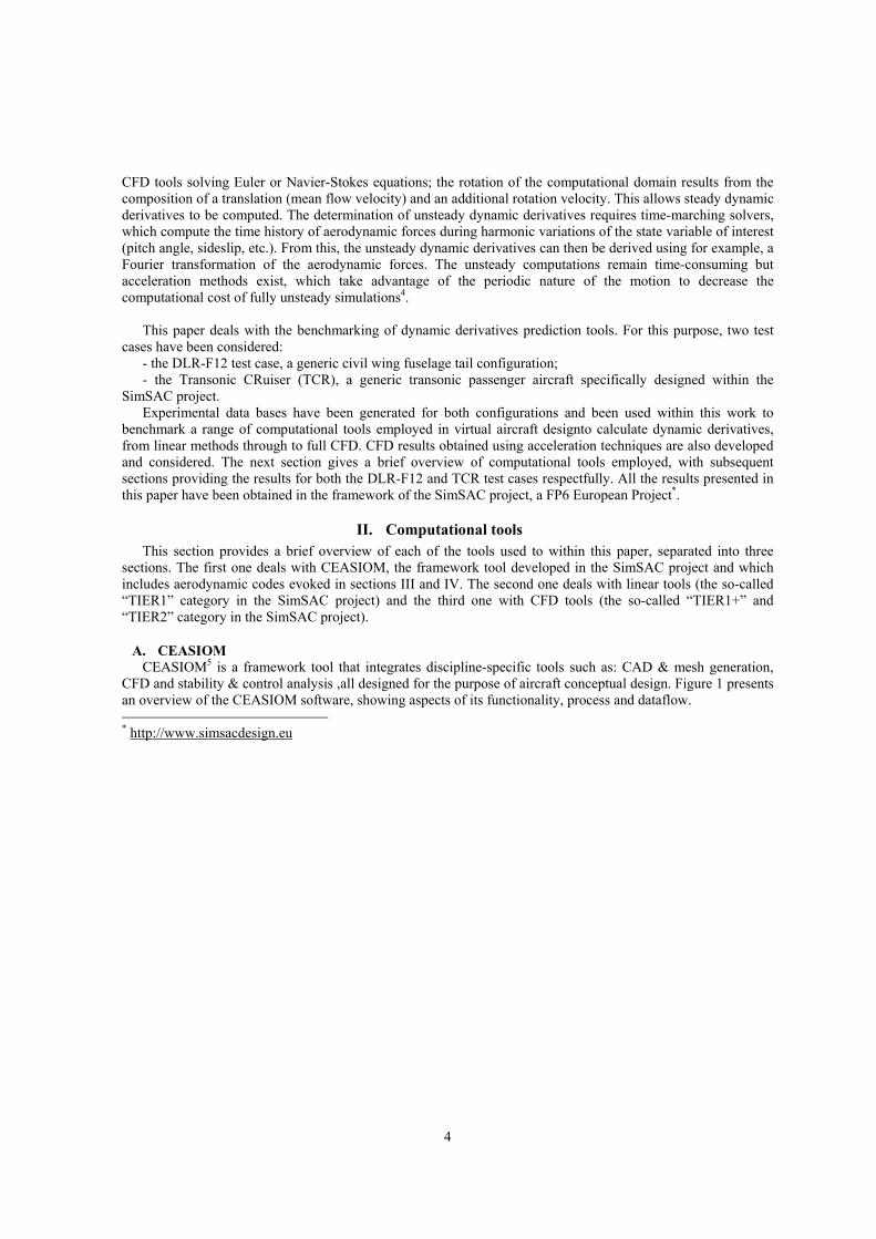
Figure 19. Components of the TCR model.

The static experiments were executed for various configurations of the model: Canard = On/Off, Vertical Tail

= On/Off. In the case of Canard=On variation of its deflection angle φc from -30 to +10° with step of 5° was investigated.

- a dynamic, small amplitude investigation of dynamic derivatives Pitch, Roll and Yaw: ± 3°, at frequency 0.5, 0.75, 1.0, 1.25 and 1.5 Hz for angles of attack varying from -10

to 40° with step of 2°. These experiments were performed on the forced angular oscillations dynamic rig OVP-102B – Fig. 20 and 21.

Heave oscillations: 0.10m at frequency 1.25, 1.5, 1.75 and 2.0 Hz for angles of attack varying from -10 to 40°

with step of 5°. These experiments were aimed to measure CN and Cm derivatives and were executed in the

PPK-103 dynamic rig. - a dynamic, large amplitude investigation of total nonlinear aerodynamic characteristics Pitch, amplitude 10, 20°, at frequency 0.5, 1.0, and 1.5 Hz for mean angles of attack 8 and 18°. Yaw, amplitude 15°, at frequency 0.5, 1.0, and 1.5 Hz for mean angles of attack 6, 10, 14, 20 and 24°. All the tests were carried out at a wind tunnel flow velocity V∞=40 m/s, corresponding to a Reynolds number

Re=0.78x106, without any transition triggering on the lifting surfaces of the model. The balance allowed five components to be measured (the drag was not measured). The reference point of the balance corresponded to the model center of gravity.

1. Static Aerodynamics Characteristics

The canard significantly contributes to the total lift force for incidences higher than 10°. For the undeflected canard case, the pitching moment versus angle of attack (Figure 22) shows a negative slope (nose down when α increases) up to α=6º, then a first break after which the slope sign changes, due to the continuously increasing lift of the canard, upstream of the reference point (nose up). Then a second break takes place, with a loss of efficiency at approximately α=20º which suggests massive flow separation. The locations of these two breaks depends on the canard deflection. The lateral stability derivative Cn indicates a loss of directional stability at angles of attack α>25º.

21

Figure 20. Forced angular oscillations dynamic rig OVP-102B used in the TsAGI T103 wind tunnel during the TCR model tests.

Figure 21. TCR model on the small amplitude roll motion mechanism.

−10 0 10 20 30 40−0.5

0

0.5

1

1.5

2Aerodynamic model: TCR

α (deg)

CN

, Cm

Canard= − 30o

Canard= − 15o

Canard= − 10o

Canard= − 5o

Canard= 0o

Canard= +5o

Canard= +10o

−10 0 10 20 30 40

−0.5

−0.4

−0.3

−0.2

−0.1

0

0.1

0.2Aerodynamic model: TCR

α (deg)

Cm

Canard= − 30o

Canard= − 15o

Canard= − 10o

Canard= − 5o

Canard= 0o

Canard= +5o

Canard= +10o

Canard= Off

Figure 22. Influence of canard and canard deflection φc on TCR model normal force and pitching

moment.

2. Small amplitude forced oscillations characteristics The small amplitude oscillations are dedicated to the determination of dynamic derivatives , given in Table 7.

Table 7. Static and dynamic derivatives measured during small amplitude oscillations. Pitch

CN CNCNq Cm CmCmq

Yaw cosCY cosCYCYr cosCl cosClClr cosCn cosCnCnr

Roll sinCY sinCYCYp sinCl sinClCl p sinCn sinCnCnp

Pitch oscillations were performed for reduced frequencies k=0.012, 0.023 and 0.035. The influence of the

canard on the pitch damping is very small, except at incidences α=20º where massive flow separation is thought to take place and leads to a positive damping (“anti damping”) (Fig. 23). The influence of the canard deflection φc was investigated: positive canard deflection moved the positive damping region to lower incidences, and increased the effect. The influence of the motion frequency was found to be small for mean angles of attack up to

2nd break

1st break

22

12/15° depending on the canard deflection. For higher angles of attack, the normal force dynamic derivative exhibits a stronger dependency on the motion frequency than the pitching moment derivative.

−20 −10 0 10 20 30 40 50−2

−1

0

1TCR: VT=On, f=1.0 Hz

Cm

α

−20 −10 0 10 20 30 40 50−30

−20

−10

0

10

20

Cm

q + C

mα’

α (deg)

Canard=Off

Canard=0o

Figure 23. Influence of the canard on the pitching moment static and dynamic derivatives (f=1.0Hz). The dynamic derivatives corresponding to rolling motion are relatively constant for angles of attack lower

than α=20º, whatever the configuration employed, as shown in Figure 24.. For higher incidences, a nonlinear behaviour appears, strongly influenced by the motion frequency. A nonlinear increase of roll damping is observed for incidences α>20º.

−10 0 10 20 30 40−0.4

−0.2

0

0.2

0.4TCR Model

CY

β sin

α

−10 0 10 20 30 40−4

−2

0

2

CY

p+C

Yβ’

sinα

α (deg)

Canard=Off, VT=OffCanard=Off, VT=On

Canard=0o, VT=On

−10 0 10 20 30 40−0.2

−0.1

0

0.1

0.2TCR Model

Clβ

sin

α

−10 0 10 20 30 40−3

−2

−1

0

1

2

Clp

+C

lβ’si

nα

α (deg)

Canard=Off, VT=OffCanard=Off, VT=On

Canard=0o, VT=On

−10 0 10 20 30 40−0.2

−0.1

0

0.1

0.2TCR Model

Cnβ

sin

α

−10 0 10 20 30 40−0.1

0

0.1

0.2

0.3

Cnp

+C

nβ’si

nα

α (deg)

Canard=Off, VT=OffCanard=Off, VT=On

Canard=0o, VT=On

Figure 24. Influence of canard and vertical tail on static and dynamic derivatives for a roll motion –

f=1.0Hz.

23

Yaw oscillations were conducted for three geometric configurations of the TCR, with and without canard and

vertical tail. For the wing+fuselage configuration, the yaw damping derivative ( cosCnCnr ) was

identified as being close to zero for incidences up to α=20°; then a strong damping effect was observed up to α=35° and finally ‘anti’ damping for higher incidences as shown in Figure 25.. The addition of the vertical tail resulted in negative damping at low angles of attack. The situation is aggravated in the anti damping region (very high incidences), which could be due to interactions between the fuselage nose vortices and the tail. The influence of the canard improves the yaw damping performance at high angles of attack. As with the pitch and rolling motions, a strong influence of the yaw motion frequency was observed for α>20º, especially for the canard-on configurations.

3. Plunge forced oscillations

Plunge forced oscillations allow the pure derivatives to be measured directly. Different configurations (without and with vertical tail, without and with canard at different deflections) were tested. The addition of the

undeflected canard to the TCR model increases the CN (from negative -8.5 to positive +2.2 at zero incidence,

f=1.5 Hz) and the Cm (from negative +6.6 to positive +18.0 at zero incidence, f=1.5 Hz) as shown in Figure

26. The influence of the motion frequency on the dynamic derivatives is small.

−20 −10 0 10 20 30 40 50−1

−0.5

0

0.5TCR: f=1.0 Hz

CY

β cos

α

−20 −10 0 10 20 30 40 50

−2

0

2

4

6

CY

r−C

Yβ’

cosα

α (deg)

Canard=Off VT=OffCanard=Off VT=On

Canard=0o VT=On

−20 −10 0 10 20 30 40 50−0.2

−0.1

0

0.1

0.2TCR: f=1.0 Hz

Clβ

cos

α

−20 −10 0 10 20 30 40 50−2

0

2

4

Clr−

Clβ

’cosα

α (deg)

Canard=Off VT=OffCanard=Off VT=On

Canard=0o VT=On

−20 −10 0 10 20 30 40 50−0.3

−0.2

−0.1

0

0.1

0.2TCR: f=1.0 Hz

Cnβ

cos

α

−20 −10 0 10 20 30 40 50−1.5

−1

−0.5

0

0.5

1

Cnr

−C

nβ’co

sα

α (deg)

Canard=Off VT=OffCanard=Off VT=On

Canard=0o VT=On

Figure 25. Influence of canard and vertical tail on static and dynamic derivatives for a yaw motion –

f=1.0Hz

24

−10 0 10 20 30 400

1

2

3

4PPK−103 rig. TCR model, Canard=Off/On, f=1.50 Hz

CN

α

−10 0 10 20 30 40−20

0

20

40

α (deg)

CN

α’

Canard=Off

Canard=0o

−10 0 10 20 30 40−2

−1

0

1PPK−103 rig. TCR model, Canard=Off/On, f=1.50 Hz

Cm

α

−10 0 10 20 30 40−10

0

10

20

30

40

α (deg)

Cm

α’

Canard=Off

Canard=0o

Figure 26. Influence of canard on static and dynamic derivatives for a plunge motion – f=1.5Hz

Comparisons between the out-of-phase derivatives obtained during plunge motion and the small amplitude

pitch oscillations are depicted in Figure 27. The difference between the “OVP 102B” and the “PPK-103” results

is attributable to the pure rotary derivatives qCN and qCm .

−10 0 10 20 30 400

1

2

3

4PPK−103 rig. TCR model, Canard=0o, f=1.50 Hz

CN

α

PPK−103OVP−102B

−10 0 10 20 30 40−20

0

20

40

α (deg)

CN

α’ C

Nq+

CN

α’

−10 0 10 20 30 40−2

−1

0

1PPK−103 rig. TCR model, Canard=0o, f=1.50 Hz

Cm

α

PPK−103OVP−102B

−10 0 10 20 30 40−30

−20

−10

0

10

20

α (deg)

Cm

α’ C

mq+

Cm

α’

Figure 27. Compared out-of-phase derivatives obtained during plunge motion and small amplitude

pitch oscillations – TCR with undeflected canard

4. Large amplitude oscillations characteristics Large amplitude oscillations were carried out in order to investigate the nonlinear aerodynamic characteristics

in off design conditions with presence of flow separation and/or vortical flows. Pitch and yawing motions were performed.

With respect to the pitch oscillations, whilst the canard-off TCR configuration exhibited a classical hysteresis

effect without any strong nonlinear dynamic effects, the addition of the canard lead to severe unsteady effects, not only for angles of attack in the region of α=20º (previously identified as a condition with a massively separated flow over the canard) but also for lower angles of attack as shown in Figure 28. These nonlinear dynamic effects are relaxed for negative deflections of the canard. For non-zero sideslip angles, the dynamic effects on the lateral/directional aerodynamic coefficients were found to be very limited for angles of attack α<20º, and significant for higher incidences (Figure 29).

25

−10 0 10 20 30 40−0.35

−0.3

−0.25

−0.2

−0.15

−0.1

−0.05

0

0.05

0.1

0.15Aerodynamic model: TCR, Canard = 0o, β = 0o, f=1.5 Hz

α (deg)

Cm

Steady

α0=8o, Aα=10o

α0=8o, Aα=20o

α0=18o, Aα=10o

α0=18o, Aα=20o

−10 0 10 20 30 40

−0.02

−0.01

0

0.01

0.02

0.03

0.04

Aerodynamic model: TCR, Canard = 0o, β < 0, α0=18o, Aα=20o

α (deg)

Cl

Steady β=−6o

f = 0.5 Hzf = 1.0 Hzf = 1.5 Hz

Steady β=−10o

f = 0.5 Hzf = 1.0 Hzf = 1.5 Hz

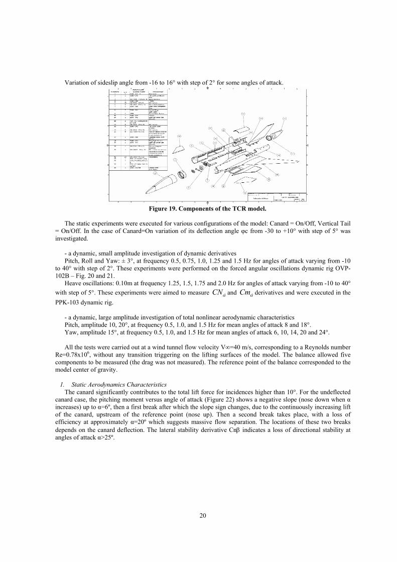
Figure 28. Pitching moment evolution for 2 sets of large amplitude pitch oscillations – TCR with canard, φc=0º, f=1.5Hz.

Figure 29. Rolling moment evolution for 2 sideslip angles during large amplitude pitch oscillations – TCR with canard, φc=0º.

Dynamic effects during yaw oscillations were found to be close to those identified during small amplitude

oscillations, with an increasing nonlinearity when the angle of attack is increased. In order to quantify whether, and to what extent, the traditional linear mathematical model of aerodynamics

based on rotary and unsteady aerodynamic derivatives concept was valid to represent large amplitude oscillations, this model was used to consider static characteristics and dynamic derivatives measured during small amplitude oscillations for the corresponding angles of attack and frequency. This allowed “simulated” forces and moments to be constructed. Results are presented in Figure 30. For the pitch oscillations, it can be seen that the simulation fits relatively well with the experimental data, except for incidences for which flow separation on the canard has been identified. For the rolling moment (during yaw oscillations), the agreement between simulated and experimental measurements is qualitatively good, despite the severe conditions considered.

−10 0 10 20 30 40−0.3

−0.25

−0.2

−0.15

−0.1

−0.05

0

0.05

0.1Aerodynamic model: TCR, Canard = 0o, β = 0o, f=0.5 Hz

α (deg)

Cm

Steady

α0=18o, Aα=10o Experiment

α0=18o, Aα=20o Experiment

α0=18o, Aα=10o Simulation

α0=18o, Aα=20o Simulation

Figure 30. Linear simulations based on the measured dynamic derivatives compared to large amplitude

oscillation measurements – pitch case (top) – yaw case (bottom). From these comparisons, it can be concluded that the classical dynamic derivative approach/model works

well given the design conditions. It is also applicable for a significant part of off-design conditions. Although the modelling error increases the trends in handling quality criteria can be correctly determined. Finally, it has been shown that the linear model based on dynamic derivatives cannot be used for the prediction of aerodynamic forces in the transient range of angles of attack for which the flow on the canard becomes separated.

C. Benchmark comparisons with CFD results With its canard configuration and the rich experimental data base available, the TCR configuration represents

a challenging test case of high interest with which to validate aerodynamic prediction tools. Within the SimSAC consortium, several partners generated results for the configuration with different solvers, the objective being to build an aerodynamic database at both low speed and for the intended cruise Mach number (M=0.97).

26

1. Static Aerodynamics Characteristics

Reference 29 describes more specifically some static results obtained with three solvers (NSMB, PMB and EDGE) and their comparison with the experimental data, focusing on the pitching moment and the trimmed conditions. It indicates that the first break in the pitching moment curve (Figure. 22) is well reproduced by Euler and RANS computations, whilst the second break, due to flow separation on the canard, is fairly well predicted by RANS solvers using structured well-resolved computational grids (Figure. 31 – for which the reference point has been changed compared to Figure. 22).

Figure 31. Pitch moment for the TCR canard configuration. M = 0.115, β = 0°, φc = 0° - (extract from 28).

2. Dynamic Derivatives

Dynamic derivatives has also been computed for the TCR configuration with different tools. A pitching motion has been simulated for the configuration with undeflected canards at 0° angle of attack. Fig. 32 illustrates the surface meshes developed for TORNADO/CEASIOM, SMARTCAD and EDGE codes.

Figure 32. View of the meshes for low/medium fidelity analysis of the TCR aircraft –

TORNADO/CEASIOM (left) SMARTCAD (centre), unstructured Euler EDGE (right) Results are presented in Tab. 8. As far as the experimental data is concerned, two motion frequencies are

included and exhibit significant differences between results at f=1.5Hz and f=1.0Hz. It is also observed that the contribution is of the same order of magnitude as the rotary component, with the same sign for the normal force derivative and the opposite sign for the pitching moment derivative. The effect of the canard on these derivatives is dramatic and the sign of the component to the normal force derivative changes for the canard-off configuration.

27

The “Native UNST” computations compare very well with experimental data for the full out-of-phase derivatives. However, the detailed analysis of each component and q indicate that significant differences exist, especially on the pitching moment terms. These differences are much higher than those observed for conventional configurations; they could originate from the bad prediction of the canard effect (including interaction between canard and wing). Significant differences between the “TORNADO/CEASIOM” and the “Native Unst” can also bbe observed. The results from SMARTCAD are in a good agreement with the “Native Unst” ones. It can be concluded that the linear tools do not predict correctly the individual components of the out-of-phase derivatives for the TCR configuration. This is likely to be linked with the high swept angle of the wing and with the canard. This is a significant difference with the DLR-F12 configuration, for which VLM tools were quite satisfactory.

As far as CFD results are concerned, Euler and URANS results are presented. The EDGE result gives a very good prediction of the pitching moment terms, including for each of the two components. Surprisingly, the result on the normal force derivatives is similar to the ones obtained with vortex lattice methods. The result obtained with PMB is in good agreement with the experimental data.

Table 8. Dynamic derivatives for the TCR configuration – pitch motion.

Linear tools CFD tools Experiment (*) SMART

CAD Native UNST*

TORNADO/ CEASIOM*

EDGE (ROM) Euler**

PMB URANS FFT f=1.0Hz

f=1.5Hz f=1.0Hz

qCN 5.70 6.14 (6.30)

6.22 4.01 (15.01)

CN 0.63 0.71 (-0.74)

0.42 -0.16 2.16 (-8.51)

CNCNq

6.34 6.85 (5.56)

6.06 7.34 6.17 (6.45)

7.02 (7.29)

qCm -6.64 -7.41 (-5.57)

-24.42 -24.46 (-11.28)

Cm 0.79 1.10 (1.24)

-0.31 19.19 17.98 (6.59)

CmCmq -5.85 -6.31 (-4.33)

-5.22 -3.8 -6.48 (-4.69)

-5.78 (-5.14)

* V∞=40m/s – M∞=0.12 – α=0º – Figures under round brackets are related to the canard-off configuration – Figures in italic are not measured but are obtained by difference. ** M∞=0.65 – α=0º

Numerical simulations for the TCR wind tunnel model were also investigated using the unsteady time

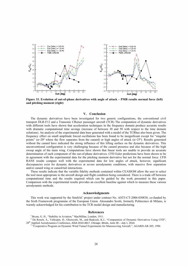
accurate PMB solver performing forced harmonic motions in pitch. The flow was modelled using the RANS equations and the k-ω with vortex correction was the adopted turbulence model. The frequency of the applied motion was 1 Hz. The dynamic derivatives for the normal force and pitching moment coefficients were estimated by processing the solution in the time domain using a developed FFT algorithm and a linear regression model was also implemented, providing very similar values to the frequency domain technique. A good agreement between numerical and experimental data is achieved up to about 10° mean angle of attack a shown in Figure 33. The magnitude of the force and moment dynamic derivatives is overpredicted at 10°, as identified by the spike in the numerical values..

It is believed that the numerical simulation of the unsteady motion is affected by the proximity to the first break in the static moment curve (Figure 22), which in turn is a challenging feature to predict using a steady state analysis. At high angle of attack, the most important observation is the positive damping measured in a narrow region at approximately 20° mean angle of attack. The numerical simulations predicted a very similar dip with negative-damping, though delayed at higher angles of incidence. It was found2 that the prediction of the second break in the static moment curve and in the positive damping dip are delayed by the same amount. Ccanard flow separation is the amenable mechanism to both situations.

28

Figure 33. Evolution of out-of-phase derivatives with angle of attack – PMB results normal force (left) and pitching moment (right)

V. Conclusion The dynamic derivatives have been investigated for two generic configurations, the conventional civil

transport DLR-F12 and a Transonic CRuiser passenger aircraft (TCR) The computation of dynamic derivatives with different tools have shown that acceleration techniques in the frequency domain produce accurate results with dramatic computational time savings (increase of between 30 and 50 with respect to the time domain solutions). An analysis of the experimental data base generated with a model of the TCRhas also been given. The frequency effect on small amplitude forced oscillations has been found to be insignificant except for “singular points” (α=20º where the flow separates from the canard) or high angles of attack (α>25º). Results generated without the canard have indicated the strong influence of this lifting surface on the dynamic derivatives. This unconventional configuration is very challenging because of the canard presence and also because of the high sweep angle of the main wing. Computations have shown that linear tools are unable to provide an accurate determination of each component of the out-of-phase derivatives. CFD Euler predictions have been shown to be in agreement with the experimental data for the pitching moment derivative but not for the normal force. CFD RANS results compare well with the experimental data for low angles of attack, however, significant discrepancies exist for dynamic derivatives at severe aerodynamic conditions, with massive flow separation and/or canard wing or canard/tail interactions.

These results indicate that the variable fidelity methods contained within CEASIOM allow the user to select the tool most appropriate to the aircraft design and flight condition being considered. There is a trade off between computational time and the results required which can be guided by the work presented in this paper. Comparison with the experimental results provides an excellent baseline against which to measure these various aerodynamic methods.

Acknowledgments This work was supported by the SimSAC project under contract No. AST5-CT-2006-030838, co-funded by the Sixth Framework programme of the European Union. Alessandro Scotti, formerly Politecnico di Milano, is warmly acknowledged for his contribution to the TCR model design and manufacturing.

References 1 Bryan, G. H., “Stability in Aviation,” MacMillan, London, 1911. 2 Da Ronch, A., Vallespin, D., Ghoreyshi, M., and Badcock, K.J., “Computation of Dynamic Derivatives Using CFD”,

28th Applied Aerodynamics Conference, AIAA-2010-4817, Chicago, Illinois, June 28 – July 1, 2010. 3 “Cooperative Program on Dynamic Wind Tunnel Experiments for Manoeuvring Aircraft.”, AGARD-AR-305, 1996

29

4 Da Ronch, A., Ghoreyshi, M., Badcock, K.J., Gortz, S., Widhalm, M., and Dwight, R., “Linear Frequency Domain and Harmonic Balance Predictions of Dynamic Derivatives”, 28th Applied Aerodynamics Conference, AIAA-2010-4699, Chicago, Illinois, June 28 – July 1, 2010.

5 von Kaenel, R., Rizzi, A., Oppelstrup, J., Goetzen, T., Ghoreyshi, M., Cavagna, L., and Bérard, A., “CEASIOM: Simulating Stability & Control with CFD/CSM in Aircraft Conceptual Design”, Paper 061, in 26th Int'l Congress of the Aeronautical Sciences, Anchorage, Alaska, Sept 2008.

6 Drela M. ”AVL 3.26 User Premier”, http://web.mit.edu/drela/Public/web/avl 7 Drela M., “Integrated Simulation Model for Preliminary Aerodynamic, Structural and Control Law Design of Aircraft”,

AIAA Paper 99 1394, 1999. 8 Cavagna, L., Ricci, S., and Riccobene, L., “A Fast Tool for Structural Sizing, Aeroelastic Analysis and Optimization in

Aircraft Conceptual Design”, 12th AIAA/ISSMO Multidisciplinary Analysis and Optimization, AIAA-2009-2571. 9 Cavagna, L. , Ricci, S., and Travaglini, L.,”NeoCASS: an integrated tool for structural sizing, aeroelastic analysis and

MDO at conceptual design level”, AIAA Atmospheric Flight Mechanics, 2-5 Aug. 2010, Toronto, Ontario, Canada 10 “Aerodynamics, stability and controllability of supersonic aircraft.” Under edition of G.S. Bushgens. Moscow, Nauka,

1998, 811pp. (in Russian). 11 Begovschitz, V., Khrabrov, A., Kolinko, K., and Machulsky, J., “UNST: Package of Interactive Calculation of Steady

and Unsteady Aerodynamic Characteristics of Aircraft”, User Manual, TsAGI, Zhukovsky, 1993. 12 Melin, T., “TORNADO a Vortex-Lattice MATLAB implementation for Linear Aerodynamic Wing Applications”,

Master Thesis, Royal Institute of Technology (KTH), Department of Aeronautivs, Stockholm, December 2000. http://www.ave.kth.se 13 Gerhold, T., Galle, M., Friedrich, O., and Evans, J., “Calculation of Complex Three-Dimensional Configurations employing the DLR TAU-Code,” AIAA Paper 97-0167, 1997.

14 J. Bastin, G. Rogé, “A multidimensional Fluctuation Splitting Scheme For The Three Dimensional Euler Equations”, M2AN, Vol 33, no 6, pp. 1241-1259, 1999

15 L. Daumas, F. Chalot, N. Forestier and Z. Johan, “Industrial Use of Linearized CFD Tools for Aeroelastic Problems”, IFASD 2009-054, International Forum on Aeroelasticity and Structural Dynamics, Seattle, WA, June 21–25, 2009. 16 L. Cambier and J.-P. Veuillot, “Status of the elsA CFD Software for Flow Simulation and Multidisciplinary Applications” AIAA 2008 664.

17 Eliasson, P., Weinerfelt, P., and Nordström, J., “Application of a Line-implicit Scheme on Stretched Unstructured Grids”, AIAA-2009-0163.

18 Eliasson, P., Weinerfelt, P., “Recent Applications of the Flow Solver Edge”, Proceedings to 7th Asian CFD conference, Bengalore, India, 2007.

19 Cavagna, L., Quaranta, G., and Mantegazza, P., “Application of Navier-Stokes simulations for aeroelastic assessment in transonic regime”, Computers & Structures, vol. 85, n. 11-14, pag.818-832, 2007

20 Rodden, W.P., and Gesling, J.P., “Application of oscillatory Aerodynamic theory to estimation of stability derivatives”, Journal of Aircraft, vol 7, n 3, 1970, pag. 272—275

21 Badcock, K. J., Richards, B. E. and Woodgate, M. A., ”Elements of Computational Fluid Dynamics on Block Structured Grids using Implicit Solvers”, Progress in Aerospace Sciences, Vol. 36, 2000, pp. 351-392.

22 Woodgate, M., and Badcock, K. J., “Implicit Harmonic Balance Solver for Forced Motion Transonic Flow”, AIAA Journal, Vol. 47, 2008, pp. 893-901.

23 Vos, J.B., Rizzi, A.W., Corjon A., Chaput, E., and Soinne, E., “Recent Advances in Aerodynamics inside the NSMB (Navier-Stokes Multiblock) Consortium”, AIAA paper 98-0225, 1998.

24 Hübner, A., Bergmann, A., and Loeser, T., “Experimental and Numerical Investigations of Unsteady Pressure Distributions and Aerodynamic Forces on Moving Transport Aircraft Configurations”, 47th AIAA Aerospace Sciences Meeting, AIAA-2009-0091, Orlando, Florida, January 5-8, 2009.

25 Mialon, B., Ben Khelil, S., Huebner, A., Jouhaud, J.C., Rogé, G., Hitzel, S., Badcock, K.J., Eliasson, P., Khrabov, A., Lahuta, M., “European Benchmark on Numerical Prediction of Stability and Control derivatives”, 27th Applied Aerodynamics Conference, AIAA-2009-4116, San Antonio, Texas, June 22-25, 2009.

26 Rizzi, A., Ricci, S., Cavagna, L., Tomac, M., Scotti, A., Puelles, A., and Riccobene, L., “Designing a TCR aircraft by simulation: from specification to WT test,” International Symposium on Coupled Methods in Numerical Dynamics, Split, Croatia, September 16–19, 2009.

27 Cavagna, L., Ricci, S., and Scotti, A., “Conceptual Design of a Three Surface Aircraft Including Aeroelastic Constraints,” International Forum on Aeroelasticity and Structural Dynamics, IFASD-2009-019, Seattle, Washington, June 21-25, 2009.

28 Rizzi, A., Goetzendorf-Grabowski, T., Vos, J., Mieszalski, D., Da Ronch, A., Tomac, M., and Ghoreyshi, M., “Creating Aero-Databases by Adapted Fidelity CFD Coupled with S&C Analysis to predict Flying Qualities,” paper in special technology session, CEAS European Air & Space Conference, Manchester, Great Britain, 26-29 Oct 2009.

29 Eliasson, P., Vos, J., Da Ronch, A., Zhang, M., and Rizzi, A., “Virtual Aircraft Design of TransCruiser – Computing Break Points in Pitch Moment Curve”, 28th Applied Aerodynamics Conference, AIAA-2010-4366, Chicago, Illinois, June 28 – July 1, 2010.