Validation of airflow measurement in ducts using Laser ... · Validation of airflow measurement in...

Validation of airflow measurement in ducts using Laser Doppler Anemometry and Computational Fluid Dynamics modelling

A. Mayes1, S. Mitchell1, J. Missenden1 & A. Gilbert2

1London South Bank University, UK 2BSRIA Instrument Solutions, UK

Abstract

The problem of airflow measurement is of interest to Building Services Engineers to allow for the effective commissioning and validation of predictive procedures. The velocity distribution in a square section duct (400 mm x 400 mm) was investigated using a Laser Doppler Anemometer (LDA) to determine the velocity distribution and volumetric flow rate in the system, and to compare it with CFD and theoretical predictions (for both square and circular sections). The procedure has revealed a number of practical issues involved in the measurement of such air flows involving an LDA, including boundary flow measurement issues, and the consistency of results. A standard Computational Fluid Dynamics (CFD) package was also used to model the same flow regime, and agreement was obtained with the LDA results for a range of flow rates. Of particular interest was the detailed distribution of modelled and measured velocities across the duct, and the ways in which these compared with the commonly assumed one-seventh power law relationship for turbulent flows. The detailed nature of the observations made allowed investigation of the suitability of power laws for the circular case, and enabled assessment of whether an alternative exponent or method of predicting such flows would be more appropriate in air flow modelling. The study shows the comparison of velocity distribution in a square duct and theoretical similarly sized circular duct. Keywords: Laser Doppler Anemometer, LDA, airflow, Computational Fluid Dynamics, CFD, log-tchebycheff, one-seventh power law, turbulent flow, boundary layer, internal flow.

Advances in Fluid Mechanics VIII 243

www.witpress.com, ISSN 1743-3533 (on-line) WIT Transactions on Engineering Sciences, Vol 69, © 2010 WIT Press

doi:10.2495/AFM10 1021

1 Introduction

The provision of good quality experimental data is essential for calibrating and validating mathematical models of airflow. Such models may be used for important applications in building services engineering, including airtightness, ventilation, air conditioning and refrigeration. Reliable data improves confidence in the use of mathematical models (generally Computational Fluid Dynamics, or CFD models), and enables design engineers to investigate the effects of installing, removing or altering the arrangement of fans, ducts and other ventilation devices, without expensive physical testing. A Laser Doppler anemometer (LDA) allows the non-intrusive measurement of air velocity. When used in a confined environment such as a duct, in which the air velocities are reasonably constant over time, measurements at a series of points across the section of flow can be integrated to give the volumetric flow rate. In addition, such results can provide important information about the variation in velocity across the duct, including near the edges (duct surfaces). Care must be taken to allow for the variation between instantaneous and time-averaged velocities, due to turbulence, by extended measurement. In order to verify the results from the LDA, CFD models can be used to picture the flow processes that occur throughout the cross section for a range of flow conditions. These models have enjoyed considerable exposure in recent years to a wide variety of flow problems in a range of engineering disciplines, beyond building services engineering. In this study, a LDA (Dantec FlowExplorer BSA F60) was used to observe the distribution of velocity in a duct of square cross section, in order to obtain the velocity distribution and so deduce volumetric flow rates for a range of airflow conditions. Comparisons were made of some of the results with the output of the CFD model (FLUENT, ANSYS, v12.0). The aim of the study was to see if the results of the CFD model were sufficiently in agreement with measurement to allow its use in studies of ducted air flow, supplemented where appropriate by the proper use of an LDA. In addition, the commonly assumed power law relationship of the turbulent flow region of a circular duct was considered.

2 Duct sections investigated

Airflow through a square duct of cross-section 400 x 400 mm was investigated using both LDA and CFD methods. In addition, a circular section was examined using CFD only. The experimental apparatus is shown in Figure 1. An Air Supply Rig provided air to the square duct. The rig consisted of a variable speed fan that directed air through an orifice plate, and into a box containing three resistance screens beyond which was a square opening. The duct was placed at the opening creating a step-change in the cross sectional area into the duct. In order to reduce the effects of jetting, hexagonal mesh sections of 100 mm overall length were incorporated to condition the flow at the inlet and outlet of the duct. The LDA was used to measure the velocity profile in the duct, and was controlled using a PC interfaced with the LDA as well as with the 3-dimensional traverse controller, allowing for accurate and repeatable positional control of the

244 Advances in Fluid Mechanics VIII


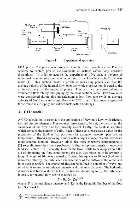
Figure 1: Experimental apparatus.

LDA probe. The probe was projected into the duct through a clear Perspex window to capture precise measurements of airflow without any intrusive disruptions. In order to acquire the experimental LDA data, a traverse of individual velocity measurements according to the Log-Tchebycheff rule was made [1]. This method creates a profile of measuring points such that the average velocity of the internal flow, over the whole cross section, is equal to the arithmetic mean of the measured points. This can then be converted into a volumetric flow rate by multiplying by the cross sectional area. Two flow rates were considered during this investigation: a low flow rate (with an average velocity of 0.620 m/s) and a high flow rate (5.761 m/s). This range is typical of those found in air supply and extract ducts within buildings.

3 CFD model

A CFD calculation is essentially the application of Newton’s Law, with friction, to fluid discrete elements. This requires three items to be set; the mesh size, the steadiness of the flow and the viscosity model. Firstly, the mesh is specified which contains the number of cells. Each of these cells possesses a value for the properties of the fluid at that position (for example, velocity, pressure, or temperature). Broadly speaking, a mesh with a larger number of cells provides a more accurate solution. However, this is also more expensive computationally [2] so preliminary tests were performed to find an optimum mesh arrangement (and see Section 3.1). Secondly, to allow the flow profile to develop without the aid of simulating the flow conditioners, the duct was modelled to be arbitrarily long. A length of 20m was deemed sufficient; this equates to 50 duct (hydraulic) diameters. Thirdly, the turbulence characteristics of the airflow at the outlet and inlet were specified. The characteristics can be defined in a number of ways, one of which is to use the turbulence intensity and hydraulic diameter. The hydraulic diameter is defined as shown below (Section 4). According to [3], the turbulence intensity for internal flow can be specified as:

81Re16.0 I (1) where ‘I’ is the turbulence intensity and ‘Re’ is the Reynolds Number of the flow (see Section 4.1).



3.1 Boundary layer

In preliminary tests, the wall-adjacent boundary layer had been simulated using a ‘non-equilibrium wall function’. This involved using a large cell size to capture this region. However, the boundary layer is of interest and, as such, the mesh has been refined to capture this region in multiple smaller cells. Instead of using a simple wall function, an enhanced wall treatment was used. This allowed the boundary layer behaviour to be captured. However, the problem with this approach is the number of cells required and the quality of these cells. Naturally, to make the cells small enough in one dimension to capture sufficient detail in the few mm of the boundary layer is at odds with the relatively long cells required to model a long duct. This leads to cells possessing a very large aspect ratio, which is undesirable as it could affect convergence and accuracy. However, length-wise partitioning of the cells would quickly lead to a model containing a huge number of cells. The greater the number of cells, the more demanding the model will be in terms of computing power and time. A preliminary investigation was performed to deduce a suitable CFD mesh. This had to be fine enough to include the near-wall behaviour where, due to the length of the duct, fine meshes at the boundary could easily lead to either long and thin cells, or far too many cells. The double-precision solver was activated to help deal with cells with high aspect ratio [3]. The k-ε realizable turbulence model was used to calculate the solution.

4 Theory

4.1 Square and circular duct relationship

For two ducts to have full similitude, they must have the same geometry and the same Reynolds Number, relating inertial to viscous forces. A square duct and a circular duct do not share geometries. However, to compare the flows the Reynolds Numbers could be equated:

hccc

hsss

DuDu ReRe , (2)

where ‘Res’ and ‘Rec’ are the Reynolds Numbers of the square and circular ducts, respectively; ‘ūs’ and ‘ūc’ are the average velocities; and ‘Dhs’ and ‘Dhc’ are the hydraulic diameters (see eqn (4)). At constant atmospheric conditions, density, ‘ρ’, and viscosity, ‘μ’, are constant. Therefore, the above equation reduces to a mean velocity, diameter equation:

hcchss DuDu . (3)

The hydraulic diameter, used to allow non-circular ducts to be treated as such, is given by:

P

ADh

4 (4)



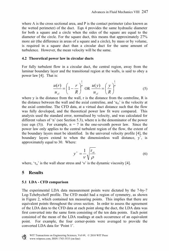
where A is the cross sectional area, and P is the contact perimeter (also known as the wetted perimeter) of the duct. Eqn 4 provides the same hydraulic diameter for both a square and a circle when the sides of the square are equal to the diameter of the circle. For the square duct, this means that approximately 27% more air (the difference in areas of a square and a circle), by mass or by volume, is required in a square duct than a circular duct for the same amount of turbulence. However, the mean velocity will be the same.

4.2 Theoretical power law in circular ducts

For fully turbulent flow in a circular duct, the central region, away from the laminar boundary layer and the transitional region at the walls, is said to obey a power law [4]. That is:

n

cl R

r

u

ru1

1)(

OR

n

cl R

y

u

yu1

)(

(5)

where y is the distance from the wall, r is the distance from the centreline, R is the distance between the wall and the axial centreline, and ‘ucl’ is the velocity at the axial centreline. The CFD data, at a virtual duct distance such that the flow was fully developed, and the theoretical power law fit were compared. This analysis used the standard error, normalised by velocity, and was calculated for different values of ‘n’ (see Section 5.3), where n is the denominator of the power (see eqn (5)). For example, n = 7 in the one-seventh power law. Since the power law only applies to the central turbulent region of the flow, the extent of the boundary layers must be identified. In the universal velocity profile [4], the boundary layers extend to when the dimensionless wall distance, y+, is approximately equal to 30. Where:

1

y (6)

where, ‘τω’ is the wall shear stress and ‘υ’ is the dynamic viscosity [4].

5 Results

5.1 LDA - CFD comparison

The experimental LDA data measurement points were dictated by the 7-by-7 Log-Tchebycheff profile. The CFD model had a region of symmetry, as shown in Figure 2, which contained ten measuring points. This implies that there are equivalent points throughout the cross section. In order to assess the agreement of the LDA data to the CFD data at each point along the duct, the LDA data was first converted into the same form consisting of the ten data points. Each point consisted of the mean of the LDA readings at each occurrence of an equivalent point. For example, the four corner-points were averaged to provide the converted LDA data for ‘Point 1’.



-200

0

200

-200 0 200

Point 1Point 2Point 3Point 4Point 5Point 6Point 7Point 8Point 9Point 10Symmetry Region

.

Figure 2: Symmetries and point locations with the CFD model.

The normalised standard error for each duct distance was found by comparing the corresponding ten points. However, each contribution was weighted by the number of instances of that point (for example, the four ‘Point 1’s and eight ‘Point 6’s). This enabled identification of the duct distance at which there was a highest agreement between CFD and experimental LDA data. By plotting how the normalised standard error changes over the length of the virtual duct, the distance at which this value is smallest can be found. This implies that this virtual duct distance has the best agreement with the experimental LDA data. The distance was found to be at 2.75 m and 5 m for the low speed and high speed tests respectively. These normalised standard error results shown in Figure 3.

0

0.01

0.02

0.03

0.04

0.05

0.06

0.07

0.08

0.09

0.1

0 5 10 15 20

Distance along duct (m)

Nor

mal

ised

Sta

ndar

d Er

ror

High Speed Low Speed

Figure 3: Normalised standard errors between CFD and LDA data.



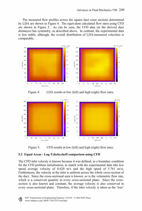
The measured flow profiles across the square duct cross sections determined by LDA are shown in Figure 4. The equivalent calculated flow rates using CFD are shown in Figure 5. As can be seen, the CFD data (at the derived duct distances) has symmetry, as described above. In contrast, the experimental data is less stable, although, the overall distribution of LDA-measured velocities is comparable.

Figure 4: LDA results at low (left) and high (right) flow rates.

Figure 5: CFD results at low (left) and high (right) flow rates.

5.2 Equal Areas - Log-Tchebycheff comparison using CFD

The CFD inlet velocity is known because it was defined, as a boundary condition for the CFD problem initialisation, to match with the experimental data (the low speed average velocity of 0.620 m/s and the high speed of 5.761 m/s). Furthermore, the velocity at the inlet is uniform across the whole cross-section of the duct. Since the cross-sectional area is known, so is the volumetric flow rate, which is a conserved quantity in every cross-sectional plane. Since the cross-section is also known and constant, the average velocity is also conserved in every cross-sectional plane. Therefore, if the inlet velocity is taken as the ‘true’



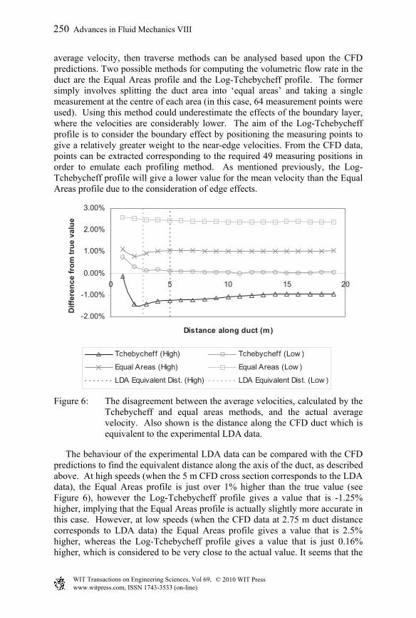
average velocity, then traverse methods can be analysed based upon the CFD predictions. Two possible methods for computing the volumetric flow rate in the duct are the Equal Areas profile and the Log-Tchebycheff profile. The former simply involves splitting the duct area into ‘equal areas’ and taking a single measurement at the centre of each area (in this case, 64 measurement points were used). Using this method could underestimate the effects of the boundary layer, where the velocities are considerably lower. The aim of the Log-Tchebycheff profile is to consider the boundary effect by positioning the measuring points to give a relatively greater weight to the near-edge velocities. From the CFD data, points can be extracted corresponding to the required 49 measuring positions in order to emulate each profiling method. As mentioned previously, the Log-Tchebycheff profile will give a lower value for the mean velocity than the Equal Areas profile due to the consideration of edge effects.

-2.00%

-1.00%

0.00%

1.00%

2.00%

3.00%

0 5 10 15 20

Distance along duct (m)

Diff

eren

ce fr

om tr

ue v

alue

Tchebycheff (High) Tchebycheff (Low )

Equal Areas (High) Equal Areas (Low )

LDA Equivalent Dist. (High) LDA Equivalent Dist. (Low )

Figure 6: The disagreement between the average velocities, calculated by the Tchebycheff and equal areas methods, and the actual average velocity. Also shown is the distance along the CFD duct which is equivalent to the experimental LDA data.

The behaviour of the experimental LDA data can be compared with the CFD predictions to find the equivalent distance along the axis of the duct, as described above. At high speeds (when the 5 m CFD cross section corresponds to the LDA data), the Equal Areas profile is just over 1% higher than the true value (see Figure 6), however the Log-Tchebycheff profile gives a value that is -1.25% higher, implying that the Equal Areas profile is actually slightly more accurate in this case. However, at low speeds (when the CFD data at 2.75 m duct distance corresponds to LDA data) the Equal Areas profile gives a value that is 2.5% higher, whereas the Log-Tchebycheff profile gives a value that is just 0.16% higher, which is considered to be very close to the actual value. It seems that the



percentage error changes along the duct, approaching a constant value (see Figure 6). This figure also shows that the Tchebycheff method always estimates a lower value than the Equal Areas method. This is expected, see [5] and as described above.

5.3 Theoretical power law

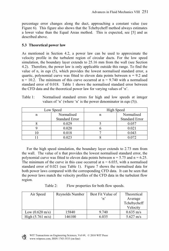
As mentioned in Section 4.2, a power law can be used to approximate the velocity profile in the turbulent region of circular ducts. For the low speed simulation, the boundary layer extends to 25.16 mm from the wall (see Section 4.2). Therefore, the power law is only applicable outside this range. To find the value of n, in eqn (5), which provides the lowest normalised standard error, a quartic, polynomial curve was fitted to eleven data points between n = 9.2 and n = 10.2. The minimum of this curve occurred at n = 9.740 with a normalised standard error of 0.018. Table 1 shows the normalised standard error between the CFD data and the theoretical power law for varying values of ‘n’.

Table 1: Normalised standard errors for high and low speeds at integer values of ‘n’ (where ‘n’ is the power denominator in eqn (5)).

Low Speed High Speed n Normalised

Standard Error n Normalised

Standard Error 8 0.029 5 0.057 9 0.020 6 0.021

10 0.018 7 0.043 11 0.023 8 0.072

For the high speed simulation, the boundary layer extends to 2.73 mm from the wall. The value of n that provides the lowest normalised standard error, the polynomial curve was fitted to eleven data points between n = 5.75 and n = 6.25. The minimum of the curve in this case occurred at n = 6.035, with a normalised standard error of 0.021 (see Table 1). Figure 7 shows the normalised data for both power laws compared with the corresponding CFD data. It can be seen that the power laws match the velocity profiles of the CFD data in the turbulent flow region.

Table 2: Flow properties for both flow speeds.

Air Speed Reynolds Number Best Fit Value of ‘n’

Theoretical Average

Tchebycheff Velocity

Low (0.620 m/s) 15840 9.740 0.635 m/s High (5.761 m/s) 146100 6.035 5.627 m/s



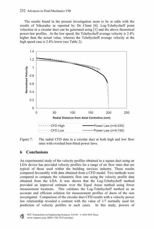
The results found in the present investigation seem to be at odds with the results of Nikuradse as reported by De Chant [6]. Log-Tchebycheff point velocities in a circular duct can be generated using [1] and the above theoretical power-law profiles. At the low speed, the Tchebycheff average velocity is 2.4% higher than the actual value, whereas the Tchebycheff average velocity at the high speed case is 2.4% lower (see Table 2).

0

0.2

0.4

0.6

0.8

1

1.2

1.4

0 50 100 150 200 250Radial Distance from Axial Centreline (mm)

Nor

mal

ised

Vel

ocity

CFD High Power Law (n=6.035)CFD Low Power Law (n=9.740)

Figure 7: The radial CFD data in a circular duct at both high and low flow rates with overlaid best-fitted power laws.

6 Conclusions

An experimental study of the velocity profiles obtained in a square duct using an LDA device has provided velocity profiles for a range of air flow rates that are typical of those used within the building services industry. These results compared favourably with data obtained from a CFD model. Two methods were compared to compute the volumetric flow rate using the velocity profile data obtained from the LDA. It was shown that the Log-Tchebycheff method provided an improved estimate over the Equal Areas method using fewer measurement locations. This validates the Log-Tchebycheff method as an accurate and efficient solution for measurement profiles of ducts of the size investigated. Comparison of the circular duct CFD results with a velocity power law relationship revealed a contrast with the value of 1/7 normally used for prediction of velocity profiles in such cases. In this study, powers of



approximately 1/6 (low speed) and 1/10 (high speed) were found to be more appropriate. This has implications for the application of the 1/7 power law in the prediction of the velocity profiles in circular ducts. In addition, the use of the derived power laws to extract theoretical Log-Tchebycheff velocity values produces encouraging results (Section 5.3). Further work would help develop the methods for using the LDA, such as spacing and near-wall reflection and combination with CFD modelling, in order that greater confidence can be obtained in prediction of the flow data in air ducts of this kind. This study has shown that there is a definite correlation between the experimental, computational and theoretical data; the span at low speed is 0.015 m/s and at high speed is 0.134 m/s. Assuming the LDA measurement is the true value, this equates to a maximum disagreement of 2.4% above at low speed and 2.4% below at high speed. Deviations from the ideal in level of agreement could be attributed to the complex nature of turbulent flow, assumptions used in the computational modelling process and possible inadequacies in the experimental setup. However, this work does validate the use of CFD as a tool for predicting airflow within ducts of the sizes considered.

Acknowledgements

This work was part funded by the UK Government via the Technology Strategy Board under its Knowledge Transfer Partnership programme [KTP 7139]. BSRIA Instrument Solutions provided the laboratory facilities including the LDA.

References

[1] BS ISO 3966:2008, Measurement of fluid flow in closed conduits. Velocity area method using Pitot static tubes, 2008.

[2] Versteeg, H.K. & Malalasekera, W., An Introduction to Computational Fluid Dynamics, Pearson Education Limited, 2007.

[3] FLUENT 12.0 User’s Guide, ANSYS, 2009. [4] Benedict, R.P., Fundamentals of Pipe Flow, Wiley, 1980. [5] ISO 5802:2009, Industrial fans - Performance testing in situ, 2009. [6] De Chant, L.J., The venerable 1/7th power law turbulent velocity profile: a

classical nonlinear boundary value problem solution and its relationship to stochastic processes, Applied Mathematics and Computation, 161, pp. 463-474, 1985.

[7] Albrecht, H.-E., Borys, M., Damaschke, N. & Tropea, C., Laser Doppler and Phase Measurement Techniques, Springer-Verlag Berlin Heidelberg, 2003.

[8] Sherwin, K., Horsley, M., Thermofluids, Chapman & Hall, 1996. [9] Rae, W.H., Jr., Pope, A., Low-speed wind tunnel testing, Wiley, 1999. [10] LMNO Engineering, Research and Software Ltd. website,

www.lmnoeng.com/index.shtml



Validation of airflow measurement in ducts using Laser ... · Validation of airflow measurement in...

Documents

Transcript of Validation of airflow measurement in ducts using Laser ... · Validation of airflow measurement in...