VALIDATING DESIGN METHODS FOR SIZING SUBMARINE...

Warship 2014: Naval Submarines & UUV’s, 18-19 June 2014, Bath, UK

© 2014: Defence Research and Development Canada DRDC-RDDC-2014-P24

VALIDATING DESIGN METHODS FOR SIZING SUBMARINE TAILFINS M. C. Bettle, Defence Research and Development Canada – Atlantic (DRDC), Canada SUMMARY A significant design challenge to providing the desired stability, manoeuvrability, and control characteristics for a submarine is sizing the tailfins. A recent analysis of a generic submarine shape using the DRDC submarine simulation program (DSSP) showed the submarine to be very unstable in both the horizontal and vertical planes. This geometry-based tool estimates hydrodynamic coefficients, predicts stability characteristics, simulates six degrees of freedom (6 DOF) manoeuvres, and determines safe operating envelopes. It uses analytical/semi-empirical methods which are amenable to rapid analysis and design; its simulations run more than an order-of-magnitude faster than real time. DSSP was used to find the appropriate adjustment to X-rudder size to achieve a desirable level of stability while retaining adequate maneuverability and control. The manoeuvring characteristics for the original and revised models are compared by performing several 6 DOF manoeuvring simulations with DSSP. To validate these analyses without incurring the large expense of experiments, computationally intensive computational fluid dynamics (CFD) predictions are compared with the DSSP load predictions. NOMENCLATURE S Exposed planform area of a tailplane (m2) b Tailplane span, from hull centreline (m) c Tailplane chord (m) CB Centre of buoyancy CG Centre of gravity Gh Stability index for horizontal plane motion Gv Stability index for vertical plane motion ks Sail efficiency ksp Sailplane efficiency KWB Tailplane efficiency L Overall submarine hull length (m) m’ Vehicle mass, non-dimensionalized by M’ Non-dimensional pitching moment, about y N’ Non-dimensional yawing moment, about z

Non-dimensional rotation rate about y-axis Non-dimensional rotation rate about z-axis

rM Maximum hull radius (m). ReL Reynolds number based on L. R Turning radius (m) u, v, w Vehicle velocity in x, y, and z directions (m s-1) U Vehicle speed (m s-1) Uc Critical speed for vertical plane stability (m s-1) Y’ Non-dimensional lateral force, in y-direction x, y, z Body axis coordinate directions xG’ Axial location of CG, non-dimensionalized by L x0,y0,z0 Inertial (earth-fixed) axes Z’ Non-dimensional normal force, in z-direction α Angle of attack β Angle of drift

Tailplane deflection for yaw control (Eq. 7) (°) Tailplane deflection for pitch control (Eq. 8) (°)

θ Submarine pitch angle (degrees) ζ Damping ratio ρ Density of water Ω Fluid domain rotation rate Forces and moments are non-dimensionalized by

and , respectively.

1. INTRODUCTION Submarines require tailfins for dynamic stability and control, components that must be sized properly to achieve adequate stability without compromising manoeuvrability. These performance characteristics are determined by the hydrodynamic loads on the vehicle and, especially, the tailfins. Predicting these loads during design is challenging. Although the theory for evaluating lift on isolated wings is well-developed, the lift generated by tailfins is complicated by the fact that they operate in a relatively thick hull boundary [1]. Estimates for submarine hydrodynamic loads can be obtained from several semi-empirical load estimation methods that have been developed from a combination of theory and empirical databases. These run very fast on modern computers and are thus useful for preliminary tailfin design. Many of these methods are incorporated in the Defence Research and Development Canada (DRDC) Submarine Simulation Program (DSSP) [2-4]. DSSP can be used to calculate loads on captive models, derive hydrodynamic coefficients, simulate tactical manoeuvres, and generate Manoeuvring Limitation Diagram (MLD) curves. The effect of changes to tailfin geometry on the manoeuvring characteristic of a submarine can be readily simulated with simple geometry input to DSSP. Alternatively, computational fluid dynamics (CFD) can provide numerical predictions for submarine manoeuvring characteristics with much better modelling of the flow physics. Other studies have shown relatively good agreement between CFD and experiment for submarine hydrodynamic load predictions (see for example [5-10]). However, CFD is orders-of-magnitude more expensive in terms of both the time to set-up simulations and computational effort relative to DSSP. This expense makes it difficult to use CFD early in the design process, but it is useful for validating semi-empirical methods at an intermediate stage to possibly


DRDC-RDDC-2014-P24 © 2014: Defence Research and Development Canada

further refine a design before even more expensive experimental testing is conducted. Also, CFD is the best available method for estimating the effect of Reynolds number scaling from model to full-scale. In the present work, DSSP is used to study the effect of tailfin size on the stability and manoeuvring characteristics of a preliminary-design generic submarine shape. The DSSP predictions are used to recommend an improved design. Both the preliminary design and improved design are then compared with CFD simulations at model-scale. 2. SUBMARINE GEOMETRY The generic BB1 submarine hull form, shown in Figure 1, is the baseline geometry for this work. This preliminary design was created by Australia’s Defence Science and Technology Organisation (DSTO) based on concept design guidelines given by Joubert [11]. It has not been optimized for hydrodynamic/manoeuvring performance. The full-scale BB1 hull form has an overall hull length of 70.2 m and a maximum hull diameter of 9.6 m. Quick et al. [12] present wind tunnel data for the BB1 bare hull. The BB1 sail is based on a NACA0017 airfoil section with a rounded cap and is fitted with sailplane control surfaces. It has 4 aft control surfaces with a thickness-to-chord ratio of approximately 16% arranged in an “X” configuration. The BB2, also shown in Figure 1, is a variant of the BB1 designed by the Maritime Research Institute Netherlands (MARIN) subsequent to performing stability and manoeuvring analyses of the BB1 similar to the one presented in this paper. Relative to the BB1, it has larger aft control surfaces and a thicker sail (NACA0022 section) that is moved slightly forward. The hull and deck casing were unchanged from the BB1 model.

Figure 1. BB1 and BB2 hull forms showing body coordinate system directions used for analysis.

The BB1 and BB2 tailfin planforms are shown in more detail in Figure 2. The BB1 tailfins extend to the maximum hull radius, b = rM, (4.8 m at full-scale) while the BB2 tailfins extend approximately to the corners of the hull bounding box at b ~ 1.42 rM from the hull centreline. The BB2 tailfins also have a fixed (non-deflecting) pedestal (dashed line in Figure 2), which accounts for just over 40% of the total planform area. Overlaid on this plot are variations to the BB1 span b and chord c considered for the present study; these variations all have the same quarter chord location. 3. OPEN LOOP STABILITY The open loop dynamic stability of submarines for horizontal-plane and vertical-plane motions is assessed using a small-perturbation analyses about zero flow incidence as discussed, for example, by Lambert [13], Hoyt and Imlay [14], Feldman [15] and MacKay [1]; a short summary is provide here. By solving the linearized equations of motion using Laplace transforms, the following stability criteria are obtained for horizontal-plane and vertical plane motion, respectively:

(1)

(2)

where and are horizontal-plane and vertical-plane stability indices, respectively, is non-dimensional mass, is the non-dimensional axial location of the vehicle centre of gravity (CG), , , , , , ,

, and are non-dimensional stability derivatives. Non-dimensionalizing and the form of the stability derivatives follow standard notation [16]. The above stability criterion for horizontal plane motion applies at any speed. A vehicle with a negative is dynamically unstable. The physical implication of this is that the submarine will not follow a straight course in the absence of autopilot or operator control; any slight disturbance will cause it to start turning in the horizontal plane. Stability is desired for controllability but excessive stability will result in poor manoeuvrability / turning ability. As a result, submarines are often designed to have a marginal amount of horizontal stability, and even a slight amount of open loop instability may be acceptable. Feldman [15] suggests that a Gh value of around 0.2 provides good dynamic performance in the horizontal plane. In contrast with Gh, the Gv criteria for vertical plane stability applies only to the limit of infinite forward speed. This is because there is a hydrostatic restoring moment in the vertical plane that stabilizes the boat at lower speeds, so long as the vehicle centre of gravity (CG) is below its centre of buoyancy (CB). This



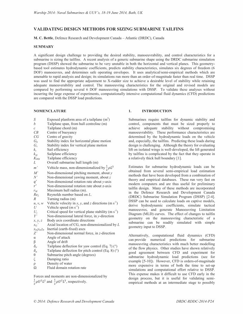
Figure 2. Variations of the BB1 tailfin considered in this study, coloured by DSSP predictions for submarine directional stability: red indicates dynamic instability in both the horizontal and vertical planes, orange (1.2-00) indicates marginal stability in the horizontal plane and instability in the vertical plane, and blue and black indicate stability in both planes. stabilizing hydrostatic effect is invariant with speed while hydrodynamic forces increase with speed. At high speeds, hydrodynamic terms dominate and the hydrostatic effect becomes negligible so that stability is achieved if , analogous to the horizontal plane stability criteria. If a vehicle is stable at infinite speed, it will be stable at all speeds [15] (so long as it has static stability). At low speeds, the hydrostatic terms dominate and the only vertical plane stability criterion in the limit of zero speed is that the CG is below the CB. For vehicles with a negative Gv but having static stability, there is some critical speed Uc above which it is unstable. At intermediate speeds, the damping ratio ζ (see [1],[15]) gives an indication of the vertical-plane dynamic performance. Feldman [15] indicates that good dynamic performance in the vertical plane is achieved when Gv is in the range , and the damping ratio is around 0.7 at moderate speeds. Having a sufficient margin of open loop stability in the vertical plane is more critical than in the horizontal plane. This is because a rapid depth changing ability increases the risk of

exceeding either deep diving or near surface (covertness) limits. 3.1 Stability Analysis Reference Point The stability analysis is usually conducted using a reference point (coordinate system origin) that is at, or very close to, the CG. In some cases, stability derivatives are obtained from experiments having a reference that is some axial distance xCG from CG. This distance appears to be accounted for in Equations 1 and 2; however, the results from the present study indicate that significantly different results for Gh and Gv (up to ~50%) are obtained when using a reference point at midship (L/2 aft of nose, ~ 0.04 L aft of CG) than at the CG, as shown in Table 1 at the end of the paper. We are currently investigating this issue. Preliminary results indicate that consistent results for Gh and Gv can be obtained if the stability derivatives are first transformed to the longitudinal location of CG before using them in Equations 1 and 2 (and setting xCG to zero).



Feldman derives this transformation for rotational derivatives Zq’ and Mq’ on pages 9-10 of Reference [15]:

(3)

(4) where subscript o indicates the reference used in the experiment (or simulation, etc.) and subscript G indicates the reference is at the longitudinal location of CG. Analagous expressions can be derived for Yr’ and Nr’:

(5)

(6) Transformations for the derivatives Mw’ and Nv’ are as follows:

(7)

(8) As shown in Table 1, Gv and Gh calculated with transformed derivatives (from midship to CG) are within 4% of Gv and Gh values calculated from derivatives obtained directly with a reference at the longitudinal location of CG. The comparison is good but this preliminary finding needs further investigation. 4. FORCE ESTIMATION METHODS A brief summary of the DSSP version 5.0 methods used for the present work are provided here; additional information is available in References [2-4]. DSSP defaults were used unless otherwise specified. DSSP builds a hydrodynamic model for a submarine by breaking it into a small number of components whose individual and interactive hydrodynamics can be estimated. For the present work, the following components are input: a hull, sail, sailplanes, “X” tailfins, and (for manoeuvring simulations) a propeller. The hull geometry, including deck, is defined by the breadth and depth at axial stations, with optional input of section area and camber. An empirical prediction of in-plane hull loads is used for translation, while rotation is modelled using a combination of slender body theory and empirical function for local crossflow drag [4]. Currently, the effect of the deck is accounted for crudely with simple scaling factors of for lateral force and yawing moment; factors of 1.2 and 1.0 were used as suggested in the user input reference [6]. Work is in progress to improve the estimation of deck loads in DSSP [17]. Appendage (sail, sailplanes, tailfins, etc.) geometry is input by giving their four corner points (leading edge

root, leading edge tip, trailing edge tip, and trailing edge root), thickness-to-chord ratio, and camber. The appendage loads are estimated by modifying the incidence angle in Aucher’s [18] formulation for an isolated appendage to account for interference between the appendage and the hull it is mounted on. Different efficiency factors are applied for each type of appendage. The efficiency factor is defined as the ratio between the hydrodynamic load produced by an appendage attached to the hull and that of an equivalent appendage in isolation (mounted on a reflecting plane). The sail efficiency factor is derived from Pitts [19]:

(9) where and are the distances from an effective hull centreline to the top of the deck casing and to the tip of the sail, respectively. The effective hull centreline is shifted above the actual hull centreline by the distance from the top of the bare hull to the top of the deck casing (see Figure 7 of Reference [4]). Equation 9 estimates to be approximately 2.2 for both the BB1 and BB2. The sail efficiency factor is much larger than 1 because the local angle of attack is increased due to hull displacement and lift is carried over from the sail to the hull. The sailplane efficiency factor is estimated as follows:

(10)

where and are the deck and sailplane heights, both measured from the hull centreline. Using this estimate,

for the BB1 and BB2. The tailplane efficiency is the most influential on dynamic stability but also the most difficult to predict because the tail appendages are located in the relatively thick boundary layer of the hull afterbody [1]. DSSP50 has two methods for predicting tailplane efficiency: Dempsey’s semi-empirical method [20] and Bohlmann’s modified Spreiter Method [21]. Mackay et al. [21] review other semi-empirical methods for tailplane efficiency and find that Dempsey’s method is the most widely used. It is based on towing tank measurements with a family of 20 sets of tail appendages mounted on the Model 4621 hull form. The experiments were conducted at a Reynolds number based on hull length, ReL, of 14 million and the appendage chord Reynolds numbers, Rec, ranged from 0.3 to 1 million. The tailfin efficiency, KWB, is expressed by Dempsey as a function of ratio of tailfin span from hull centreline, b, to maximum hull radius, rM:



for and (11) and

for (12) Note that the range covered by Eq 12 covers the range of tailfin spans used in Dempsey’s experiments while Eq 11 is an extrapolation beyond that range. Dempsey’s empirical formula predicts for BB1 and

for BB2, which both have b/rM within the range covered by the experiments. Mackay et al. [21] note that Dempsey’s experiments only varied appendage span and aspect ratio without considering other potential parameters such as the hull afterbody fullness or Reynolds numbers. They compare Dempsey’s data and correlation with other historical data that indicated that Dempsey’s experiments may be at a boundary between subcritical (Rec) and supercritical fin chord Reynolds number data. The higher Reynolds number data have higher tailplane efficiency for any given b/rM ratio. They conducted experiments with three hull forms and three tailfins with different aspect ratios that confirm this trend – KWB increases up to a Reynolds number of 20 million at which point it appears to plateau. MacKay et al. also studied the effect of hull slenderness by performing wind tunnel experiments with hulls having tail cone angles ranging from 14 to 24 degrees. Their preliminary results show that increasing the fullness of the tail decreases tailplane efficiency. The 12° tail cone angle for the Model 4621 used in Dempsey’s experiments is significantly less steep than the BB1 hull form, which has a cone angle of approximately 16.5° at the tailfin location. Bohlmann’s modified Spreiter Method is a rational / physics-based approach developed to address shortcomings of existing semiempirical methods. The method derives efficiency coefficients for an equivalent triangular wing. Potential flow and thin boundary layer calculations are performed to adjust the hull radii and cone angle via the boundary layer displacement thickness. A comparison with experiments showed that the method tends to over-predict tailplane efficiency [21]. An empirical correction was added in DSSP in an effort to compensate for this; however some preliminary testing showed that this correction may be over-compensating as lower than expected KWB values were being predicted for the ‘all-moving’ type appendages. For this reason, the Dempsey method was used for all DSSP simulations for this work. The Bohlmann’s Spreiter Method will be revisited in follow-on work.

5. DSSP SIMULATIONS 5.1 STABILITY PREDICTIONS Estimates for the 8 stability derivatives in Eqs. 1 and 2 are needed to estimate the dynamic stability characteristics. DSSP has a routine that calculates Gv, Gh, ζ, and Uc whenever a “Coefficient” type simulation is performed. However, the coefficients used in the stability analysis are obtained using least-squares regression over the broad range of +/- 20 degrees for incidence and +/- 2 deg/s for angular rates. Coefficients from this regression are referred to as “manoeuvring coefficients” as they provide a good fit over the broad flow incidence range encountered in manoeuvring simulations. However, they are inaccurate estimates of the derivatives at zero incidence, which are needed for the stability analysis. DSSP is in the process of being updated to correct this. For the present study, stability derivatives were computed by conducting DSSP “Static” type simulations with the small ranges of +/- 0.01 degrees for translational flow incidence and +/- 0.07 for the normalized rotation rates and . The stability derivatives were found to vary by less than 0.1% within these small ranges. Note that when comparing with CFD results in Section 6 below, the DSSP translational stability derivatives are evaluated using load predictions at 1 degree incidence as this is the smallest incidence used for the CFD simulations. The 1 degree differencing approximation agrees with the limiting slope at zero incidence within ~3%. The CG was used as the reference point when obtaining stability derivatives and stability indices in this section. Results are compared with a reference at midship in Section 6. DSSP predictions for the effect of tailfin size on Gv and Gh for the BB1 are shown in Figure 3. The BB1 baseline model is predicted to have very large negative stability indices of Gh = -1.1 and Gv = -2.1. A vehicle with such large open loop instability will be difficult to control. Fortunately, the stability is predicted to increase quickly as the span of the BB1 tailfin is increased, and marginal stability is achieved for the horizontal and vertical planes when b ~ 1.2 m (A/ABB1 = 1.4, b/bBB1 = 1.25). When the span is extended to the corners of the hull bounding box, Gv and Gh are both predicted to be on the order of 0.3. The BB2 tailfin, which also uses this span but with a slightly larger tip chord than used for the parametric study, is predicted to have stability indices of Gh ~ 0.31 and Gv ~ 0.37, values which are close to Feldman’s recommendations for good dynamic performance (Gh ~ 0.2 and 0.5 < Gv < 0.7). Figure 3 also shows that that increasing the tailfin span is much more effective than increasing chord for increasing stability. This is expected because 1) higher aspect ratio wings are more efficient and 2) increasing span improves



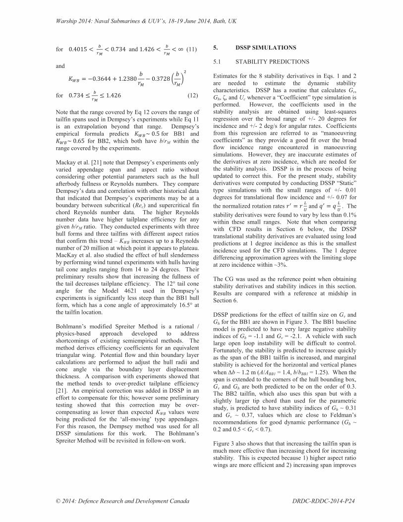
tailplane efficiency by moving more of the tail out of the hull boundary layer (see Eqs 5 and 6). The damping ratio was also calculated as a function of speed for the BB1 and BB2 as shown in Figure 4. The BB1 is estimated to have a critical velocity of 4.4 m/s, above which the submarine has a negative damping ratio and is unstable. The BB2 has a damping ratio around 0.4 for moderate speeds, which is lower than Feldman’s recommendation of 0.7, but may be sufficient depending on the controls used. The predicted damping ratio for a submarine having the BB2 tail and BB1 sail is also shown in Figure 4. The close comparison with the BB2 indicates that the changes to the sail in the BB2 revision have only a small effect on stability in the vertical plane. In the horizontal plane, Gh is reduced slightly from 0.39 to 0.31 when the BB1 sail is replaced with the BB2 sail.

Figure 3. DSSP based predictions of stability indices for the BB1, BB2, and BB1 with increments to chord and span as shown in Figure 2.

Figure 4. DSSP derived predictions for damping ratio for the BB1, BB2, and a submarine having the BB2 tail and BB1 sail.

5.2 MANOEUVRING SIMULATIONS The results from the stability analysis provide a preliminary indication of the dynamic performance of the BB1 configured with different tailfins and help determine an appropriate range of tailfin sizes. Various manoeuvring simulations were also conducted in DSSP to better assess the vehicle’s dynamic behaviour. For these simulations, the propeller is modelled as a Wageningen B-series with a pitch to diameter ratio of 1.2 for the BB1 and 0.966 for the BB2. In both cases the propeller diameter for the full-scale model is 5 meters. Note that for ‘X’ rudders, all 4 tailfins are used when steering in either the horizontal or vertical planes. The following effective rudder (yaw control) deflection and sternplane (pitch control) deflection definitions are used:

(13)

(14) where , , , are the angular deflections of the upper starboard, lower starboard, lower port, and upper port tailfins, respectively. The right-hand rule with a positive local rotation axis pointing out along the fin span is used to determine the rotation direction of each tailfin deflection, consistent with DSSP convention. A positive turns the submarine to port side and a positive

pitches the submarine down (for forward motion). 5.2 (a) Horizontal Plane Motion Horizontal plane stability is analysed by performing a Dieudonné spiral manoeuvre. Starting from straight and level flight at 10 m/s, the rudders are deflected to give

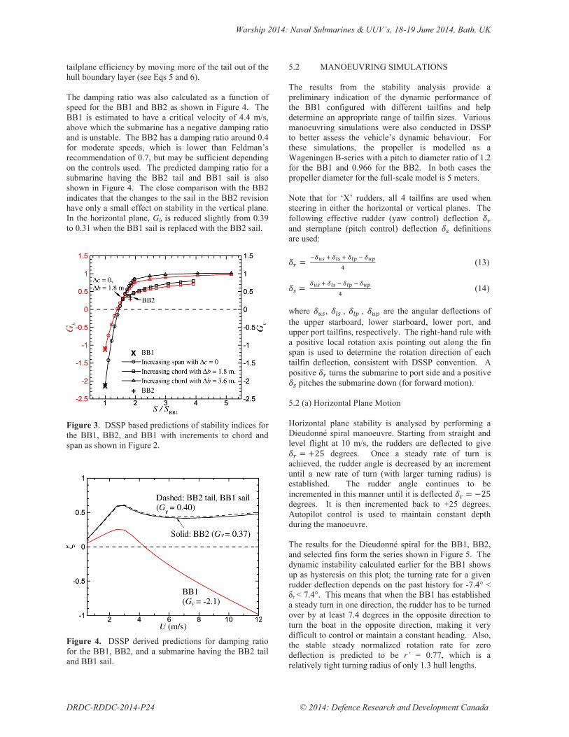
degrees. Once a steady rate of turn is achieved, the rudder angle is decreased by an increment until a new rate of turn (with larger turning radius) is established. The rudder angle continues to be incremented in this manner until it is deflected degrees. It is then incremented back to +25 degrees. Autopilot control is used to maintain constant depth during the manoeuvre. The results for the Dieudonné spiral for the BB1, BB2, and selected fins form the series shown in Figure 5. The dynamic instability calculated earlier for the BB1 shows up as hysteresis on this plot; the turning rate for a given rudder deflection depends on the past history for -7.4° < δr < 7.4°. This means that when the BB1 has established a steady turn in one direction, the rudder has to be turned over by at least 7.4 degrees in the opposite direction to turn the boat in the opposite direction, making it very difficult to control or maintain a constant heading. Also, the stable steady normalized rotation rate for zero deflection is predicted to be r’ = 0.77, which is a relatively tight turning radius of only 1.3 hull lengths.



.

Figure 5. DSSP predictions for non-dimensional turning rate versus rudder angle (Gh estimates are from DSSP).

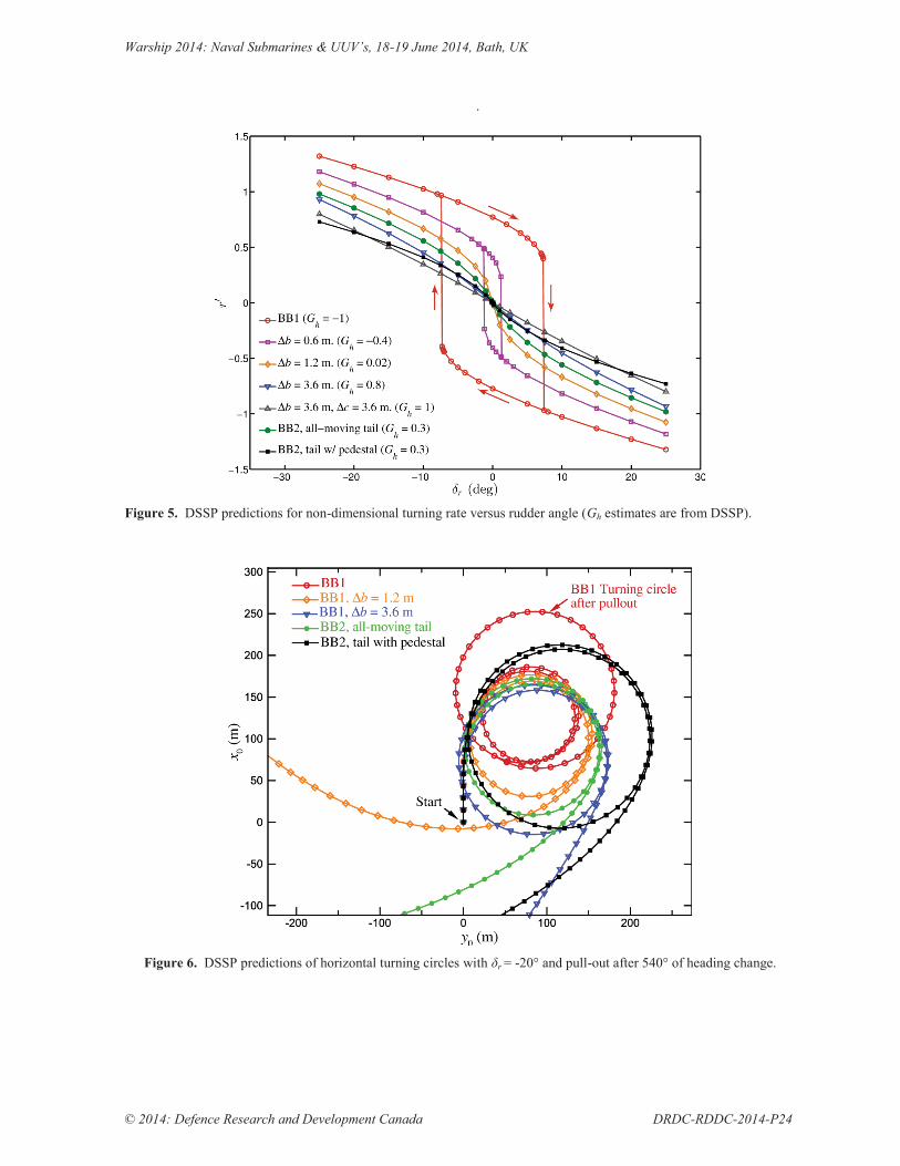
Figure 6. DSSP predictions of horizontal turning circles with δr = -20° and pull-out after 540° of heading change.



Figure 7. DSSP predictions for depth excursion (top) and pitch (bottom) during the 10°/10° vertical zig-zag manoeuvre.

The level of hysteresis decreases to zero as the tailfin span is increased by about 1.2 meters at which point the submarine is predicted to be marginally stable. Another point to note from results in Figure 5 is that the normalized rate of turn that is achieved for a given rudder angle decreases as the stability increases. There is a further decrease for the BB2 because of a fixed tailplane pedestal (see Figure 1), which reduces the loads due to tailplane deflection. Horizontal turning circle manoeuvres were also simulated. Starting from straight and level flight at 10 m/s, the rudder is deflected and held at degrees until the submarine has turned 540 degrees, at which point the rudder is returned to zero deflection. Figure 6 shows the turning circles for some of the same submarine configurations considered for the Dieudonné spiral. In agreement with the Dieudonné spiral results, the steady turning radius increases with tailfin size. However, the forward advance for the first 90 degrees of turn is reduced as tailfins are enlarged. The more stable configurations also achieve a straight course more quickly after pull-out, while the very unstable BB1cannot

pull out of the turn. A comparison of the BB2 with an identical submarine that has all moving tail fins (no fixed pedestal) is also shown in Figure 6. They both have the same dynamic stability, as evidenced by the similar behaviour upon pull-out, but DSSP predicts that the BB2 with fixed pedestal to have a 34% larger turning radius due to the reduction in movable area. 5.2 (b) Vertical Plane Zig-Zag Vertical plane manoeuvring characteristics are evaluated by performing a zig-zag manoeuvre. Starting from straight and level flight at 10 m/s, the rudders are given a δs = -10° deflection to pitch the submarine up. When a pitch angle of +10 degrees is achieved, the rudders are reversed to +10 degrees and held until the submarine achieves a -10° pitch angle. This sequence is repeated to again achieve +10° and -10° pitch angles. When a -10° pitch angle is achieved for the second time, the rudders are zeroed for the remainder of the simulation Figure 7 shows the zig-zag results for BB1 variants with selected tailfin sizes. The BB1 experiences excessively



large depth and pitch excursions of growing magnitude during the zig-zag as a result of its dynamic instability. Also, long after the planes are zeroed, it achieves a steady pitch angle of 10 degrees and an upward translation. As expected, the magnitude of overshoots decrease with increasing tailfin size due to increased dynamic stability. By comparing the BB2 (with a fixed pedestal) with an equivalent submarine having all-moving tailfins, it can be seen that the pedestal reduces the amount of overshoot in pitch. The submarine experiences a peak pitch angle magnitude of 26° with all- moving fins but only 22° with the fixed pedestal. However, the manoeuvre takes longer for the fin with pedestal due to the reduced control loads, resulting in a slightly larger depth excursion for the zig-zag phase but not for the settling phase after is zeroed. The DSSP simulations indicate that increasing span of the BB1 tailfins out to the hull bounding box will provide a good level of stability and dynamic performance. More work is needed to assess the design and benefits of using different pedestal designs and it would be interesting to see the effect it has on the safe operating limits in a manoeuvring limitation diagram [22]. The DSSP stability predictions for the BB1 and BB2 are now compared with CFD calculations. 6. CFD COMPUTATIONS 6.1 FLOW SOLVER & TURBULENCE MODELS The ANSYS CFX v12.1 flow solver was used to compute hydrodynamic loads on the fully appended BB1 and BB2 submarines. CFX solves the discretized Reynolds averaged Navier-Stokes (RANS) equations using a finite element-based finite volume method. The hydrodynamic equations for pressure and the three components of velocity are solved as a single system using a coupled solver [23,24] and the Additive Correction [25] Algebraic Multi-grid [26] procedure is used to accelerate the solution. Second order-accurate discretization is used for advection terms and double precision is used for all simulations. The Baseline Reynolds Stress (BSL-RSM) model [27] and Menter’s two-equation SST turbulence model [28] are both used in this work. Both models have been found to have reasonable agreement with experiment, though the BSL-RSM has been shown to be the superior of the two for bare hull computations [6]. This comes at the cost of solving additional turbulence transport equations, which also tends to make the BSL-RSM less stable. The BSL-RSM was initially attempted for all simulations in the work, but it had to be abandoned for the SST model with curvature correction for rotational cases due to convergence problems. Work is underway to try to achieve convergence with the BSL-RSM for all cases and compare results for the two models.

6.2 MESH AND BOUNDARY CONDITIONS 6.2 (a) Fluid Domain and Meshes A structured mesh with 8 million hexahedral cells was built around the BB2 geometry using ANSYS ICEM Hexa for discretizing the flow domain. The mesh on the submarine boundary and a section of the centre plane near the submarine are shown in Figure 8. The domain extends out to a rectangular box that has clearances from the submarine boundary of 2L on each side and top and bottom, 2L in front, and 3L behind. A similar BB2 grid with 60 million cells was created by refining by a factor of 2 in each coordinate direction in order to assess mesh sensitivity. Stability derivatives for translation obtained with each grid were all within only 0.4% of each other. For the BB1, a 10.6 million node hybrid mesh was generated using Pointwise v17.1 mesh script provided by Envenio Inc. The BB1 mesh has a similar hexahedral mesh in the near body region and approximately the same domain size as the BB2 mesh. However, surrounding the structured near-body mesh is an unstructured tetrahedral mesh layer, which is in turn surrounded by a second (coarser) hexahedral mesh region that extends out the far-field boundaries. The use of the three mesh layers is described in [6]. This baseline grid was coarsened to 4 million nodes and refined to 33.5 million nodes to assess mesh sensitivity. At β = 10°, all three grids give Y’ and N’ predictions within 0.3% of each other. All of the grids have a first node spacing that gives a y+ value of around 0.5 at ReL = 5.2 × 106. The coordinates system used for most CFD simulations have the origin on the hull axis at the intersection of the longitudinal axis of symmetry of the hull and midship (L/2 aft of the nose), with x directed forward, y to starboard and z vertically downward. However, one set of results have the origin shifted forward in the x-direction to the longitudinal CG (estimated with DSSP to be 0.039592 L and 0.039875 L forward of midship for the BB1 and BB2, respectively). 6.2 (b) Boundary Conditions Both steady translation and steady rotation simulations are performed to get the stability derivatives. In all simulations, the submarine boundary is set to a smooth no-slip wall. The following far-field boundary conditions are set for steady translation simulations:

In front of the submarine and any side, top, or bottom boundary through which far-field flow is entering the domain: Inlet with fluid velocity set to the far-field flow velocity (the negative of the submarine translational velocity). Turbulence intensity set to 1%.



Figure 8. Mesh on BB2 surface and centre plane (8.0 × 106 mesh nodes in full domain).

Sides, top, and bottom surfaces for which far-field flow is tangent or leaving the domain: “Entrainment Opening” with pressure and pressure gradient normal to the boundary set to zero. (A zero reference pressure is used).

Behind the submarine: Outlet with average static pressure set to zero.

Simulations for rotational derivatives are solved using a rotating frame of reference. The axis of rotation and angular rotation rate, Ω, are set to give the submarine the desired turning radius, R = L/r’, and translational velocity at the coordinate origin, u = U, v = 0, w = 0. The following boundary conditions are used for rotational simulations:

In front of the submarine: Inlet with zero velocity in the stationary frame (effectively setting velocity to –Ω × si in the rotating frame, where si is the position vector from the axis of rotation). Turbulence intensity set to 1%.

Sides, top, and bottom: “Entrainment Opening” with pressure and pressure gradient normal to the boundary set to zero.

Behind the submarine: Outlet with average static pressure set to zero.

The majority of CFD computations are conducted at a model-scale Reynolds number of ReL = 5.2 × 106 for consistency with past [12] and other ongoing collaborative work with the BB1 and BB2. A few results are also obtained at ReL = 14 × 106 for better comparison with DSSP prediction, which use Dempsey’s empirical tailplane efficiency method derived from experiments at that ReL. At the time of this writing, a single horizontal

rotation case for the BB1 has also been repeated at full-scale, ReL = 200 × 106. 6.3 RESULTS AND DISCUSSION CFD hydrodynamic load predictions for BB1 and BB2 as a function of drift angle, , normalized yaw

rate, , angle of attack, , and pitch

rate, , are compared with DSSP predictions in Figure 9. The general agreement between CFD and DSSP at model scale Reynolds numbers is considered to be good. The incremental change between BB1 and BB2 is particularly well predicted. The stability derivatives and indices computed for the two methods are shown in Table 1. The model-scale (ReL = 5.2 million and ReL = 14 million) CFD simulations agree with DSSP to within about 20% for all derivatives for both submarines, except for Yr’, which DSSP under-predicts by more than 50% (relative to CFD at ReL = 14 million). CFD also indicates that this derivative is very sensitive to Reynolds number. For the BB1, it increases by 35% from ReL = 5.2 million to 14 million, and an additional 30% from ReL = 14 million to 200 million. More simulations are needed to determine the Reynolds number effects on all of the stability derivatives. Model-scale CFD predictions for stability indices also agree qualitatively with DSSP; BB1 is predicted to be very unstable for both planes of motion while the BB2 is estimated to have Gh and Gv in the vicinity of 0.2-0.4. However, horizontal plane stability indices were found to increase significantly from ReL = 5.2 million to 14 million; Gh increases from -0.67 to -0.44 for BB1 and 0.19 to 0.36 for the BB2. More simulations are needed to assess dynamic stability at full-scale, but the single full-scale rotation simulation for the BB1 suggests the



Figure 9. DSSP and CFD predictions for in-plane hydrodynamic loads for steady translation and rotation in the horizontal and vertical planes. Red: BB1, black: BB2. ReL = 5.2 × 106 for CFD unless otherwise noted.



effect of going from ReL = 14 million to full scale is of the same magnitude as going from 5.2 million to 14 million. If this is the case, the BB1 will most likely still be dynamically unstable at full-scale but the level of horizontal-plane instability may no longer be considered unacceptable depending on the performance requirements and controller capabilities. This means tailfins sized using empirical methods obtained using model scale data, such as the Dempsey method used in this work for tailfin efficiency, are likely to be conservative in terms of stability at full-scale. However, this also means that a vehicle designed to have good dynamic performance at model scale may have excessive stability to achieve certain performance criteria, such as desired turning radius, at full scale. More work is needed to determine the Reynolds number scaling effects in order to improve predictions for full-scale stability and manoeuvring predictions. CFD is currently the best available method for this purpose. It would be useful to conduct CFD simulations for vehicles with and without the tailfins to better assess the tailplane efficiency factor used in semi-empirical methods. Also, six degrees of freedom manoeuvring simulations, such as those shown in [29-32], can also be performed at full-scale Reynolds numbers to better assess the manoeuvring performance of a given design. 7. CONCLUSIONS Classical stability analysis and numerical simulations based on widely-used semi-empirical methods predict the preliminary design of a generic submarine, the BB1, to be excessively unstable for both horizontal and vertical planes of motion. These methods predict that a good stability and manoeuvring performance can be achieved if the span of the BB1 tailfins are extended out to the hull bounding box (at a radius of ~1.4 times the hull radius for ‘X’ tailfins). This is the span selected for the tailfins on the BB2, a revision to the BB1 made by the Maritime Research Institute Netherlands (MARIN). Steady translation and rotational RANS computations were conducted to validate the semi-empirical-based predictions. Model-scale RANS computations showed good agreement with DSSP predictions for stability derivatives and stability indices Gh and Gv for both the BB1 and BB2. However, CFD computations indicate that the stability of both vehicles increases significantly with Reynolds number and that the classical semi-empirical methods likely under-predict stability at full-scale. More CFD computations are underway to complete quantifying this scaling effect. 8. ACKNOWLEDGEMENTS The author gratefully acknowledges the provision of the BB1 geometry from DSTO, the BB2 geometry from MARIN, and the Pointwise mesh script for generating the BB1 mesh from Envenio Inc.

Table 1. DSSP50 and CFD predictions for stability derivatives and indices for the BB1 and BB2.

Derivatives, reference at

midship.

BB1 BB2

DSSP CFD, ReL x 106

DSSP CFD

5.2 14 200 5.2 14

1000 Zw' -29.4 -22.5 -40.9 -36.0

1000 Mw' 13.2 14.4 9.4 9.9

1000 Zq' -3.4 -4.1 -7.5 -8.1

1000 Mq' -3.3 -3.1 -5.2 -5.2

1000 Yv' -67.9 -66.8 -69.1 -74.9 -73.5 -75.7

1000 Nv' -22.2 -23.4 -23.1 -18.5 -20.8 -19.9

1000 Yr' 1.5 2.5 3.4 4.4 5.0 4.6 6.1

1000 Nr' -3.8 -3.7 -4.0 -4.3 -5.8 -6.1 -6.8

Stability indices calculated using midship as reference point (xG' = 0.03989 and 0.03988 for BB1 and BB2, respectively), Eqs 1 & 2 :

Gh (Midship) -0.61 -0.67 -0.44 0.28 0.19 0.36

Gv (Midship) -1.3 -2.3 0.34 0.24

Stability indices obtained by first transforming stability derivatives from midship to longitudinal location of CG using Eqs 3-8:

Gh (CG)_t -0.94 -1.1 -0.66 0.35 0.24 0.44

Gv (CG)_t -1.9 -3.5 0.41 0.29

Stability indices obtained from DSSP and CFD simulations performed with a reference point at the longitudinal location of CG:

Gh (CG) -0.96 0.34 0.24

Gv (CG) -1.9 0.40 0.28

Comparison with transformations:

% diff Gh 1 -3 -3

% diff Gv 0.7 -2 -4

9. REFERENCES 1. M. Mackay, “Some Effects of Tailplane

Efficiency on Submarine Stability and Manoeuvering”. DREA TM 2001–031, Defence Research Establishment Atlantic, August 2001.

2. M. Mackay, ‘DSSP50 Build 090910

Documentation, Part 1: Guide and Tutorial’, DRDC Atlantic TM 2009-226, Defence Research and Development Canada – Atlantic, Dec. 2009.

3. M. Mackay, ‘DSSP50 Build 090910

Documentation, Part 2: Input Reference’, DRDC Atlantic TM 2009-227, Defence Research and Development Canada – Atlantic, Dec. 2009.



4. M. Mackay, ‘DSSP50 Build 090910 Documentation, Part 3: Algorithm Description’, DRDC Atlantic TM 2009-228, Defence Research and Development Canada – Atlantic, Dec. 2009.

5. C.H. Sung, T.-C. Fu, M. Griffin, and T. Huang,

‘Validation of Incompressible Flow Computation of Forces and Moments on Axisymmetric Bodies Undergoing Constant Radius Turning’, In Twenty-First Symposium on Naval Hydrodynamics, Washington, DC, 1997.

6. T.L. Jeans, G.D. Watt, A.G. Gerber, A.G.L.

Holloway, C.R. Baker, ‘High-resolution Reynolds-Averaged Navier-Stokes Flow Predictions over Axisymmetric Bodies with Tapered Tails’, AIAA Journal, 47 (1) (2009), pp. 19–32.

7. A.B. Phillips, S.R. Turnock, M. Furlong,

‘Influence of Turbulence Closure Models on the Vortical Flow Field Around a Submarine Body Undergoing Steady Drift’, Journal of Marine Science and Technology, 15 (3) (2010), pp. 201–217.

8. M. Bettle, S.L. Toxopeus, A. Gerber,

‘Calculation of bottom clearance effects on Walrus submarine hydrodynamics’, International Shipbuilding Progress, 57 (3-4) (2010), pp. 101–125.

9. S.L. Toxopeus, P. Atsavapranee, E. Wolf, S.

Daum, R. Pattenden, R. Widjaja, J.T. Zhang, and A.G. Gerber, ‘Collaborative CFD Exercise for a Submarine in a Steady Turn’, In ASME 31st International Conference on Ocean, Offshore and Artic Engineering, number OMAE2012-83573, Rio de Janeiro, Brazil, July 2012.

10. J.A. Maxwell, J.T. Zhang, G.L. Holloway, G.D.

Watt, and A.G. Gerber, ‘Simulation and Modelling of the Flow over Axisymmetric Submarine Hulls in Steady Turning’, In 28th Symposium on Naval Hydrodynamics, Pasadena, California, September 2010.

11. P. Joubert. ‘Some Aspects of Submarine Design

- Part 2. Shape of a Submarine 2026.’, Technical Report DSTO-TR-1622, Defence Science and Technology Organisation, Fishermans Bend, Victoria, Australia, Oct. 2006.

12. H. Quick, R. Widjaja, B. Anderson, B.

Woodyatt, A. D. Snowden, S. Lam, ‘Phase I Experimental Testing of a Generic Submarine Model in the DSTO Low Speed Wind Tunnel’,

DSTO-TN-1101, Defence Science and Technology Organisation, Fishermans Bend, Victoria, Australia, July 2012.

13. J.D. Lambert, ‘The Effect of Changes in the

Stability Derivatives on the Dynamic Behaviour of a Torpedo’, Admiralty Research Laboratory, Aeronautical Research Council Reports and Memoranda 3143, March 1956.

14. E.D. Hoyt and F.H. Imlay, ‘The Influence of

Metacentric Stability on the Dynamic Longitudinal Stability of a Submarine’, David W. Taylor Model Basin Report C-158, October 1948.

15. J. P. Feldman, ‘Method of Performing Captive-

Model Experiments to Predict the Stability and Control Characteristics of Submarines’, CRDKNSWC-HD-0393-25, Carderock Division Naval Surface Warfare Center, Bethesda, Maryland, June 1995.

16. J.P. Feldman, ‘DTNSRDC Revised Standard

Equations of Motion’, DTNSRDC/SPD-0393-09, David Taylor Naval Ship Research and Development Center, 1979.

17. C.R. Marshall, T.L. Jeans, A.G.L. Holloway,

G.D. Watt, ‘Hydrodynamic Forces and Moments on Slender Axisymmetric Bodies with Decks in Translation’, AIAA SciTech, National Harbour, Maryland, 52nd Aerospace Sciences Meeting, 13-17 Jan 2014.

18. M. Aucher, ‘Dvnamique des Sous-Marins’,

Sciences et Techniques de l’Armement 4e fascicule, Paris Imprimerie Nationale, 1981.

19. W.C. Pitts, J.N. Nielsen, and G.E. Kaattari, ‘Lift

and Center of Pressure of Wing-Body-Tail Combinations at Subsonic, Transonic, and Supersonic Speeds’, NACA Report 1307, 1957.

20. E.M. Dempsey, ‘Static Stability Characteristics

of a Systematic Series of Stern Control Surfaces on a Body of Revolution’, DTNSRDC Report 77-0085, August 1997.

21. M. Mackay, H.J. Bohlmann, and G.D. Watt,

‘Modelling Submarine Tailplane Efficiency’, In Challenges in Dynamics, System Identification Control and Handling Qualities for Land, Air, Sea, and Space Vehicles (RTO-MP-095), NATO RTO, May 2002.

22. D. Haynes, J. Bayliss, and P. Hardon, ‘Use of

the Submarine Research Model to Explore the Manoeuvring Envelope’, In Warship 2002: International Symposium on Naval Submarines



7, London, UK, Royal Institution of Naval Architects, 2002.

23. B.R. Hutchinson, P.F. Galpin, G.D. Raithby,

‘Application of Additive Correction Multi-Grid to the Coupled Fluid Flow Equations’, Numerical Heat Transfer, 13 (2) (1988), pp. 133–147.

24. M.J. Raw, ‘A coupled algebraic Multi-grid

Method for the 3D Navier-Stokes Equations’, In Proceedings of the Tenth GAMM-Seminar. Notes on Numerical Fluid Mechanics, Keil, Germany, 1994.

25. B.R. Hutchinson, G.D. Raithby, ‘A Multi-Grid

Method Based on the Additive Correction Strategy’, Numerical Heat Transfer, 9 (1986), pp. 511–537.

26. M.J. Raw. ‘Robustness of Coupled Algebraic

Multi-Grid for the Navier-Stokes Equation’, In 34th Aerospace and Sciences Meeting & Exhibit, number AIAA 96-0297, Reno, NV., January 1996.

27. Launder, B. E., Reece, G. J., and Rodi, W.,

‘Progress in the Development of a Reynolds-Stress Turbulence Closure’, Journal of Fluid Mechanics, Vol. 68, No. 3, Apr. 1975, pp. 537–566.

28. F.R. Menter, ‘Two-equation Eddy Viscosity

Turbulence Models For Engineering Application’, AIAA Journal, Vol. 32, No. 8, 1994, pp. 1598–1605. doi:10.2514/3.12149.

29. R. Pankajakshan, M.G. Remotigue, L.K. Taylor,

M. Jiang, W.R. Briley, and D.L. Whitfield. ‘Validation of Control-Surface Inducted Submarine Maneuvering Simulations using UNCLE’, In Twenty-Fourth Symposium on Naval Hydrodynamics, Fukuoka, Japan, July 2002.

30. M.C. Bettle, A.G. Gerber, G.D. Watt, ‘Unsteady

Analysis of the Six DOF Motion of a Buoyantly Rising Submarine’, Computers and Fluids, 38 (9) (2009), pp. 1833–1849

31. J.J. Dreyer and D.A. Boger, ‘Validation of a

Free-Swimming, Guided Multibody URANS Simulation tool’, In 28th Symposium on Naval Hydrodynamics, Pasadena, California, September 2010.

32. M.C. Bettle, A.G. Gerber, G.D. Watt, ‘Using

Reduced Hydrodynamic Models to Accelerate the Predictor-Corrector Convergence of Implicit 6-DOF URANS Submarine Manoeuvring

Simulations’, Computers & Fluids article in press, available online March 2014. http://dx.doi.org/10.1016/j.compfluid.2014.02.023

10. AUTHORS BIOGRAPHY Mark Bettle is a defence scientist at Defence Research and Development Canada, where he is specializing in submarine hydrodynamics, manoeuvring simulations, and computational fluid dynamics. He recently completed a PhD dissertation on six degrees-of-freedom submarine simulations using CFD at the University of New Brunswick, Canada.

VALIDATING DESIGN METHODS FOR SIZING SUBMARINE...

Documents

Transcript of VALIDATING DESIGN METHODS FOR SIZING SUBMARINE...