Vacuum Technology Book II Part 2
140
Part 2 The Vacuum Technology Book Volume II Know how book
Transcript of Vacuum Technology Book II Part 2

Part 2
TheVacuum
Technology
Book
Volume II
Know how book
www.pfeiffer-vacuum.comPage 2 / Part 2
Know how book
www.pfeiffer-vacuum.com Part 2 / Page 3
2 Vacuum Technology and Know how / Contents
Vacuum Technology and Know how
1 Introduction to vacuum technology
1.1 General 9
1.1.1 Vacuum – Definition . . . . . . . . . . . . . . . . . . . . . . . . . . . . . . . . . . . . . . . . . . . . . . . . . 91.1.2 Overview of vacuum . . . . . . . . . . . . . . . . . . . . . . . . . . . . . . . . . . . . . . . . . . . . . . . . . 9
1.2 Fundamentals 9
1.2.1 Definition of vacuum . . . . . . . . . . . . . . . . . . . . . . . . . . . . . . . . . . . . . . . . . . . . . . . . . 91.2.2 General gas equation . . . . . . . . . . . . . . . . . . . . . . . . . . . . . . . . . . . . . . . . . . . . . . . . 111.2.3 Molecular number density . . . . . . . . . . . . . . . . . . . . . . . . . . . . . . . . . . . . . . . . . . . . 121.2.4 Thermal velocity . . . . . . . . . . . . . . . . . . . . . . . . . . . . . . . . . . . . . . . . . . . . . . . . . . . . 121.2.5 Mean free path . . . . . . . . . . . . . . . . . . . . . . . . . . . . . . . . . . . . . . . . . . . . . . . . . . . . . 121.2.6 Types of flow . . . . . . . . . . . . . . . . . . . . . . . . . . . . . . . . . . . . . . . . . . . . . . . . . . . . . . 141.2.7 pV throughput . . . . . . . . . . . . . . . . . . . . . . . . . . . . . . . . . . . . . . . . . . . . . . . . . . . . . 151.2.8 Conductance . . . . . . . . . . . . . . . . . . . . . . . . . . . . . . . . . . . . . . . . . . . . . . . . . . . . . . 16
1.3 Influences in real vacuum systems 18
1.3.1 Contamination . . . . . . . . . . . . . . . . . . . . . . . . . . . . . . . . . . . . . . . . . . . . . . . . . . . . . 181.3.2 Condensation and vaporization . . . . . . . . . . . . . . . . . . . . . . . . . . . . . . . . . . . . . . . . 181.3.3 Desorption, diffusion, permeation and leaks . . . . . . . . . . . . . . . . . . . . . . . . . . . . . . 191.3.4 Bake-out . . . . . . . . . . . . . . . . . . . . . . . . . . . . . . . . . . . . . . . . . . . . . . . . . . . . . . . . . . 201.3.5 Residual gas composition . . . . . . . . . . . . . . . . . . . . . . . . . . . . . . . . . . . . . . . . . . . . 201.3.6 Venting . . . . . . . . . . . . . . . . . . . . . . . . . . . . . . . . . . . . . . . . . . . . . . . . . . . . . . . . . . . 20
2 Basic calculations
2.1 General 22
2.2 Calculations 22
2.2.1 Dimensioning a Roots pumping station . . . . . . . . . . . . . . . . . . . . . . . . . . . . . . . . . 222.2.2 Condenser mode . . . . . . . . . . . . . . . . . . . . . . . . . . . . . . . . . . . . . . . . . . . . . . . . . . . 252.2.3 Turbopumping stations . . . . . . . . . . . . . . . . . . . . . . . . . . . . . . . . . . . . . . . . . . . . . . 27 2.2.3.1 Evacuating a vessel to 10-8 hPa with a turbopumping station . . . . . . . . . . 27 2.2.3.2 Pumping high gas loads with turbomolecular pumps . . . . . . . . . . . . . . . . 29
2.3 Piping conductivities 30
2.3.1 Laminar conductance. . . . . . . . . . . . . . . . . . . . . . . . . . . . . . . . . . . . . . . . . . . . . . . . 302.3.2 Molecular conductance . . . . . . . . . . . . . . . . . . . . . . . . . . . . . . . . . . . . . . . . . . . . . . 30
Mechanical components in vacuum
3.1 General 32
3.2 Materials 32
3.2.1 Metallic materials . . . . . . . . . . . . . . . . . . . . . . . . . . . . . . . . . . . . . . . . . . . . . . . . . . . 33 3.2.1.1 Stainless steel . . . . . . . . . . . . . . . . . . . . . . . . . . . . . . . . . . . . . . . . . . . . . . . 33 3.2.1.2 Carbon steel . . . . . . . . . . . . . . . . . . . . . . . . . . . . . . . . . . . . . . . . . . . . . . . . . 36 3.2.1.3 Aluminum . . . . . . . . . . . . . . . . . . . . . . . . . . . . . . . . . . . . . . . . . . . . . . . . . . 363.2.2 Sealing materials . . . . . . . . . . . . . . . . . . . . . . . . . . . . . . . . . . . . . . . . . . . . . . . . . . . 36 3.2.2.1 Elastomer seals . . . . . . . . . . . . . . . . . . . . . . . . . . . . . . . . . . . . . . . . . . . . . . 36 3.2.2.2 Metal seals . . . . . . . . . . . . . . . . . . . . . . . . . . . . . . . . . . . . . . . . . . . . . . . . . . 37
Contents
3
www.pfeiffer-vacuum.comPage 4 / Part 2
2 Vacuum Technology and Know how / Contents
Contents3.3 Connections 38
3.3.1 Non-detachable connections . . . . . . . . . . . . . . . . . . . . . . . . . . . . . . . . . . . . . . . . . . 38 3.3.1.1 Welding . . . . . . . . . . . . . . . . . . . . . . . . . . . . . . . . . . . . . . . . . . . . . . . . . . . . 38 3.3.1.2 Brazing, fusing and metalizing . . . . . . . . . . . . . . . . . . . . . . . . . . . . . . . . . . 393.3.2 Detachable flange connections . . . . . . . . . . . . . . . . . . . . . . . . . . . . . . . . . . . . . . . . 40 3.3.2.1 O-Ring seals and grooves . . . . . . . . . . . . . . . . . . . . . . . . . . . . . . . . . . . . . . 40 3.3.2.2 ISO-KF flange . . . . . . . . . . . . . . . . . . . . . . . . . . . . . . . . . . . . . . . . . . . . . . . . 41 3.3.2.3 ISO-K/ISO-F flange . . . . . . . . . . . . . . . . . . . . . . . . . . . . . . . . . . . . . . . . . . . . 42 3.3.2.4 CF flange . . . . . . . . . . . . . . . . . . . . . . . . . . . . . . . . . . . . . . . . . . . . . . . . . . . 43 3.3.2.5 COF flanges . . . . . . . . . . . . . . . . . . . . . . . . . . . . . . . . . . . . . . . . . . . . . . . . . 44 3.3.2.6 Other flange standards . . . . . . . . . . . . . . . . . . . . . . . . . . . . . . . . . . . . . . . . 44 3.3.2.7 Screws . . . . . . . . . . . . . . . . . . . . . . . . . . . . . . . . . . . . . . . . . . . . . . . . . . . . . 44
3.4 Vacuum chambers 47
3.4.1 Processing – Surfaces . . . . . . . . . . . . . . . . . . . . . . . . . . . . . . . . . . . . . . . . . . . . . . . 473.4.2 Processing – Cleaning . . . . . . . . . . . . . . . . . . . . . . . . . . . . . . . . . . . . . . . . . . . . . . . 48
3.5 Components and feedthroughs 49
3.5.1 Hoses and flexible connectors . . . . . . . . . . . . . . . . . . . . . . . . . . . . . . . . . . . . . . . . . 493.5.2 Viewports . . . . . . . . . . . . . . . . . . . . . . . . . . . . . . . . . . . . . . . . . . . . . . . . . . . . . . . . . 493.5.3 Electrical feedthroughs . . . . . . . . . . . . . . . . . . . . . . . . . . . . . . . . . . . . . . . . . . . . . . 493.5.4 Other feedthroughs . . . . . . . . . . . . . . . . . . . . . . . . . . . . . . . . . . . . . . . . . . . . . . . . . 50
3.6 Valves 50
3.6.1 Valve control . . . . . . . . . . . . . . . . . . . . . . . . . . . . . . . . . . . . . . . . . . . . . . . . . . . . . . . 503.6.2 Angle valves . . . . . . . . . . . . . . . . . . . . . . . . . . . . . . . . . . . . . . . . . . . . . . . . . . . . . . . 513.6.3 Inline and diaphragm valves . . . . . . . . . . . . . . . . . . . . . . . . . . . . . . . . . . . . . . . . . . 513.6.4 Gate valves . . . . . . . . . . . . . . . . . . . . . . . . . . . . . . . . . . . . . . . . . . . . . . . . . . . . . . . . 523.6.5 Butterfly and ball valves . . . . . . . . . . . . . . . . . . . . . . . . . . . . . . . . . . . . . . . . . . . . . . 523.6.6 Gas dosing valves and gas control valves . . . . . . . . . . . . . . . . . . . . . . . . . . . . . . . . 52
3.7 Manipulators and mechanical feedthroughs 52
3.7.1 Operating principles . . . . . . . . . . . . . . . . . . . . . . . . . . . . . . . . . . . . . . . . . . . . . . . . 53 3.7.1.1 Translation sealed by diaphragm bellows . . . . . . . . . . . . . . . . . . . . . . . . . . 53 3.7.1.2 Bellows-sealed rotation . . . . . . . . . . . . . . . . . . . . . . . . . . . . . . . . . . . . . . . . 53 3.7.1.3 Magnetically coupled rotation and translation . . . . . . . . . . . . . . . . . . . . . . 54 3.7.1.4 Sealed elastomer rotation and translation . . . . . . . . . . . . . . . . . . . . . . . . . . 54 3.7.1.5 Rotation via sliding gaskets with pumped interspaces . . . . . . . . . . . . . . . . 54 3.7.2 Accuracy, repeatable precision and resolution . . . . . . . . . . . . . . . . . . . . . . . . . . . . 54 3.7.3 Technical equipment and characteristics . . . . . . . . . . . . . . . . . . . . . . . . . . . . . . . . . 55 3.7.3.1 Design features of a Z-axis precision manipulator . . . . . . . . . . . . . . . . . . . 55 3.7.3.2 Design features of an XY-axis precision manipulator . . . . . . . . . . . . . . . . . 56
4 Vacuum generation
4.1 Vacuum pumps – working principles and properties 58
4.1.1 Classification of vacuum pumps . . . . . . . . . . . . . . . . . . . . . . . . . . . . . . . . . . . . . . . 58 4.1.2 Pumping speed and throughput . . . . . . . . . . . . . . . . . . . . . . . . . . . . . . . . . . . . . . . 594.1.3 Ultimate pressure and base pressure . . . . . . . . . . . . . . . . . . . . . . . . . . . . . . . . . . . 59 4.1.4 Compression ratio . . . . . . . . . . . . . . . . . . . . . . . . . . . . . . . . . . . . . . . . . . . . . . . . . . 59 4.1.5 Pumping speed of pumping stages connected in series . . . . . . . . . . . . . . . . . . . . . 59 4.1.6 Gas ballast . . . . . . . . . . . . . . . . . . . . . . . . . . . . . . . . . . . . . . . . . . . . . . . . . . . . . . . . 59 4.1.7 Water vapor tolerance / water vapor capacity . . . . . . . . . . . . . . . . . . . . . . . . . . . . . 60 4.1.8 Sealing gas . . . . . . . . . . . . . . . . . . . . . . . . . . . . . . . . . . . . . . . . . . . . . . . . . . . . . . . . 60
www.pfeiffer-vacuum.com Part 2 / Page 5
2 Vacuum Technology and Know how / Contents
Contents 4.2 Rotary vane vacuum pumps 60
4.2.1 Design / Operating principle . . . . . . . . . . . . . . . . . . . . . . . . . . . . . . . . . . . . . . . . . . 604.2.2 Application . . . . . . . . . . . . . . . . . . . . . . . . . . . . . . . . . . . . . . . . . . . . . . . . . . . . . . . . 614.2.3 Portfolio overview . . . . . . . . . . . . . . . . . . . . . . . . . . . . . . . . . . . . . . . . . . . . . . . . . . . 61 4.2.3.1 Single-stage rotary vane vacuum pumps . . . . . . . . . . . . . . . . . . . . . . . . . . 62 4.2.3.2 Two-stage rotary vane vacuum pumps . . . . . . . . . . . . . . . . . . . . . . . . . . . . 63 4.2.3.3 Operating fluid selection . . . . . . . . . . . . . . . . . . . . . . . . . . . . . . . . . . . . . . . 66 4.2.3.4 Accessories . . . . . . . . . . . . . . . . . . . . . . . . . . . . . . . . . . . . . . . . . . . . . . . . . 66
4.3 Diaphragm vacuum pumps 68
4.3.1 Design / Operating principle . . . . . . . . . . . . . . . . . . . . . . . . . . . . . . . . . . . . . . . . . . 684.3.2 Application . . . . . . . . . . . . . . . . . . . . . . . . . . . . . . . . . . . . . . . . . . . . . . . . . . . . . . . . 684.3.3 Portfolio overview . . . . . . . . . . . . . . . . . . . . . . . . . . . . . . . . . . . . . . . . . . . . . . . . . . . 684.3.4 Accessories . . . . . . . . . . . . . . . . . . . . . . . . . . . . . . . . . . . . . . . . . . . . . . . . . . . . . . . 68
4.4 Screw vacuum pumps 69
4.4.1 Design / Operating principle . . . . . . . . . . . . . . . . . . . . . . . . . . . . . . . . . . . . . . . . . . 694.4.2 Application . . . . . . . . . . . . . . . . . . . . . . . . . . . . . . . . . . . . . . . . . . . . . . . . . . . . . . . . 694.4.3 Portfolio overview . . . . . . . . . . . . . . . . . . . . . . . . . . . . . . . . . . . . . . . . . . . . . . . . . . . 704.4.4 Accessories . . . . . . . . . . . . . . . . . . . . . . . . . . . . . . . . . . . . . . . . . . . . . . . . . . . . . . . 70
4.5 Multi-stage Roots pumps – Vacuum generation
4.5.1 Design / Operating principle . . . . . . . . . . . . . . . . . . . . . . . . . . . . . . . . . . . . . . . . . . 714.5.2 Application . . . . . . . . . . . . . . . . . . . . . . . . . . . . . . . . . . . . . . . . . . . . . . . . . . . . . . . . 714.5.3 ACP portfolio overview. . . . . . . . . . . . . . . . . . . . . . . . . . . . . . . . . . . . . . . . . . . . . . . 72 4.5.3.1 Air cooled multi-stage Roots pumps . . . . . . . . . . . . . . . . . . . . . . . . . . . . . . 72 4.5.3.2 Accessories . . . . . . . . . . . . . . . . . . . . . . . . . . . . . . . . . . . . . . . . . . . . . . . . . 73
4.6 Multi-stage Roots pumps – Vacuum processes
4.6.1 Design / Operating principle . . . . . . . . . . . . . . . . . . . . . . . . . . . . . . . . . . . . . . . . . . 744.6.2 Application . . . . . . . . . . . . . . . . . . . . . . . . . . . . . . . . . . . . . . . . . . . . . . . . . . . . . . . . 754.6.3 Load locks and noncorrosive gases . . . . . . . . . . . . . . . . . . . . . . . . . . . . . . . . . . . . . 754.6.4 Process chemistry . . . . . . . . . . . . . . . . . . . . . . . . . . . . . . . . . . . . . . . . . . . . . . . . . . 764.6.5 Harsh process chemistry . . . . . . . . . . . . . . . . . . . . . . . . . . . . . . . . . . . . . . . . . . . . . 764.6.6 Portfolio overview . . . . . . . . . . . . . . . . . . . . . . . . . . . . . . . . . . . . . . . . . . . . . . . . . . . 77 4.6.6.1 Water cooled, process pumps . . . . . . . . . . . . . . . . . . . . . . . . . . . . . . . . . . . 77 4.6.6.2 Accessories . . . . . . . . . . . . . . . . . . . . . . . . . . . . . . . . . . . . . . . . . . . . . . . . . 78
4.7 Roots vacuum pumps 78
4.7.1 Design / Operating principle . . . . . . . . . . . . . . . . . . . . . . . . . . . . . . . . . . . . . . . . . . 784.7.2 Application . . . . . . . . . . . . . . . . . . . . . . . . . . . . . . . . . . . . . . . . . . . . . . . . . . . . . . . . 80 4.7.2.1 Backing pump selection . . . . . . . . . . . . . . . . . . . . . . . . . . . . . . . . . . . . . . . . 804.7.3 Portfolio overview . . . . . . . . . . . . . . . . . . . . . . . . . . . . . . . . . . . . . . . . . . . . . . . . . . . 81 4.7.3.1 Standard pumps . . . . . . . . . . . . . . . . . . . . . . . . . . . . . . . . . . . . . . . . . . . . . . 81 4.7.3.2 Standard pumps with magnetic coupling . . . . . . . . . . . . . . . . . . . . . . . . . . 81 4.7.3.3 Explosion-protected pumps . . . . . . . . . . . . . . . . . . . . . . . . . . . . . . . . . . . . . 81 4.7.3.4 Gas circulation cooled Roots pumps . . . . . . . . . . . . . . . . . . . . . . . . . . . . . . 824.7.4 Accessories . . . . . . . . . . . . . . . . . . . . . . . . . . . . . . . . . . . . . . . . . . . . . . . . . . . . . . . 824.7.5 Pumping stations . . . . . . . . . . . . . . . . . . . . . . . . . . . . . . . . . . . . . . . . . . . . . . . . . . . 82
4.8 Side channel high vacuum pumps 83
4.8.1 Design / Operating principle . . . . . . . . . . . . . . . . . . . . . . . . . . . . . . . . . . . . . . . . . . 834.8.2 Application . . . . . . . . . . . . . . . . . . . . . . . . . . . . . . . . . . . . . . . . . . . . . . . . . . . . . . . . 834.8.3 Portfolio overview . . . . . . . . . . . . . . . . . . . . . . . . . . . . . . . . . . . . . . . . . . . . . . . . . . . 83

www.pfeiffer-vacuum.comPage 6 / Part 2
2 Vacuum Technology and Know how / Contents
Contents 4.9 Turbomolecular pumps 83
4.9.1 Design / Operating principle . . . . . . . . . . . . . . . . . . . . . . . . . . . . . . . . . . . . . . . . . . 83 4.9.1.1 Turbomolecular pump operating principle . . . . . . . . . . . . . . . . . . . . . . . . . . 84 4.9.1.2 Holweck stage operating principle . . . . . . . . . . . . . . . . . . . . . . . . . . . . . . . 86 4.9.1.3 Turbopump performance data . . . . . . . . . . . . . . . . . . . . . . . . . . . . . . . . . . . 874.9.2 Application . . . . . . . . . . . . . . . . . . . . . . . . . . . . . . . . . . . . . . . . . . . . . . . . . . . . . . . . 884.9.3 Portfolio overview . . . . . . . . . . . . . . . . . . . . . . . . . . . . . . . . . . . . . . . . . . . . . . . . . . . 89 4.9.3.1 Mechanical-bearing turbopumps . . . . . . . . . . . . . . . . . . . . . . . . . . . . . . . . . 89 4.9.3.2 Active magnetic-levitation turbopumps . . . . . . . . . . . . . . . . . . . . . . . . . . . . 90 4.9.3.3 Drives and accessories . . . . . . . . . . . . . . . . . . . . . . . . . . . . . . . . . . . . . . . . 90
5 Vacuum measuring equipment
5.1 Fundamentals of total pressure measurement 92
5.1.1 Direct, gas-independent pressure measurement . . . . . . . . . . . . . . . . . . . . . . . . . . . 925.1.2 Indirect, gas-dependent pressure measurement . . . . . . . . . . . . . . . . . . . . . . . . . . . 93
5.2 Application notes 95
5.2.1 Measuring ranges . . . . . . . . . . . . . . . . . . . . . . . . . . . . . . . . . . . . . . . . . . . . . . . . . . 955.2.2 Active vacuum gauges . . . . . . . . . . . . . . . . . . . . . . . . . . . . . . . . . . . . . . . . . . . . . . . 965.2.3 Passive vacuum gauges . . . . . . . . . . . . . . . . . . . . . . . . . . . . . . . . . . . . . . . . . . . . . . 965.2.4 Combination vacuum gauges . . . . . . . . . . . . . . . . . . . . . . . . . . . . . . . . . . . . . . . . . 96
5.3 Portfolio overview 96
5.3.1 DigiLine . . . . . . . . . . . . . . . . . . . . . . . . . . . . . . . . . . . . . . . . . . . . . . . . . . . . . . . . . . 965.3.2 ActiveLine . . . . . . . . . . . . . . . . . . . . . . . . . . . . . . . . . . . . . . . . . . . . . . . . . . . . . . . . . 995.3.3 ModulLine . . . . . . . . . . . . . . . . . . . . . . . . . . . . . . . . . . . . . . . . . . . . . . . . . . . . . . . 100
6 Mass spectrometers and residual gas analysis
6.1 Introduction, operating principle 102
6.2 Sector field mass spectrometers 103
6.2.1 Operating principle . . . . . . . . . . . . . . . . . . . . . . . . . . . . . . . . . . . . . . . . . . . . . . . . . 1036.2.2 Application notes . . . . . . . . . . . . . . . . . . . . . . . . . . . . . . . . . . . . . . . . . . . . . . . . . . 104
6.3 Quadrupole mass spectrometers (QMS) 104
6.3.1 Quadrupole mass filter . . . . . . . . . . . . . . . . . . . . . . . . . . . . . . . . . . . . . . . . . . . . . . 1046.3.2 Ion sources . . . . . . . . . . . . . . . . . . . . . . . . . . . . . . . . . . . . . . . . . . . . . . . . . . . . . . . 1076.3.3 Detectors . . . . . . . . . . . . . . . . . . . . . . . . . . . . . . . . . . . . . . . . . . . . . . . . . . . . . . . . 1106.3.4 Vacuum systems . . . . . . . . . . . . . . . . . . . . . . . . . . . . . . . . . . . . . . . . . . . . . . . . . . 1126.3.5 Inlet systems . . . . . . . . . . . . . . . . . . . . . . . . . . . . . . . . . . . . . . . . . . . . . . . . . . . . . 1126.3.6 Application notes . . . . . . . . . . . . . . . . . . . . . . . . . . . . . . . . . . . . . . . . . . . . . . . . . . 113
6.4 Portfolio overview 114
6.4.1 Advantages of Pfeiffer Vacuum mass spectrometers . . . . . . . . . . . . . . . . . . . . . . 1156.4.2 Data analysis system . . . . . . . . . . . . . . . . . . . . . . . . . . . . . . . . . . . . . . . . . . . . . . . 116

www.pfeiffer-vacuum.com Part 2 / Page 7
2 Vacuum Technology and Know how / Contents
Contents 7 Leak detection
7.1 General 118
7.1.1 Leaks and leak detection . . . . . . . . . . . . . . . . . . . . . . . . . . . . . . . . . . . . . . . . . . . . 1187.1.2 Leakage rate . . . . . . . . . . . . . . . . . . . . . . . . . . . . . . . . . . . . . . . . . . . . . . . . . . . . . . 1187.1.3 Tracer gases . . . . . . . . . . . . . . . . . . . . . . . . . . . . . . . . . . . . . . . . . . . . . . . . . . . . . . 119
7.2 Leak detection with tracer gases 119
7.2.1 Design of a leak detector with a mass spectrometer . . . . . . . . . . . . . . . . . . . . . . 1197.2.2 Design of a leak detector with a quartz window detector . . . . . . . . . . . . . . . . . . 1207.2.3 Test methods . . . . . . . . . . . . . . . . . . . . . . . . . . . . . . . . . . . . . . . . . . . . . . . . . . . . . 1217.2.4 Calibrating the leak detector . . . . . . . . . . . . . . . . . . . . . . . . . . . . . . . . . . . . . . . . . 1217.2.5 Local leak detection . . . . . . . . . . . . . . . . . . . . . . . . . . . . . . . . . . . . . . . . . . . . . . . . 1217.2.6 Integral leak detection . . . . . . . . . . . . . . . . . . . . . . . . . . . . . . . . . . . . . . . . . . . . . . 122
7.3 Application notes 122
7.3.1 Leak detection with helium . . . . . . . . . . . . . . . . . . . . . . . . . . . . . . . . . . . . . . . . . . 1227.3.2 Comparison of test results with leak detector and
quadrupole mass spectrometer . . . . . . . . . . . . . . . . . . . . . . . . . . . . . . . . . . . . . . . 123
7.4 Portfolio overview 124
7.5 Industrial leak testing 125
8 Contamination management solutions
8.1 Introduction 126
8.2 Contamination 127
8.3 The nature of AMC 128
8.4 From surface molecular contamination (SMC) to defects 128
8.5 Portfolio overview 130
www.pfeiffer-vacuum.comPage 8 / Part 2
Intr
od
uct
ion
to
vacu
um
tec
hn
olo
gy
1 Introduction to vacuum technology
Vacuum Know how
BA
CK
ING
VA
CU
UM
Lo
w V
acu
um
Lam
inar
flo
w
Ro
tary
van
e p
um
ps
Liq
uid
rin
g p
um
ps
Dia
ph
rag
m p
um
ps
Scr
oll
pu
mp
sR
oo
ts p
um
ps
Scr
ew p
um
ps
Turb
om
ole
cula
r p
um
ps
Dif
fusi
on
pu
mp
s
Sp
utt
er io
n g
ette
r p
um
ps
Cry
o p
um
ps
Mec
han
ical
+ c
apac
itiv
e m
easu
rem
ent
equ
ipm
ent
Th
erm
al c
on
du
ctiv
ity
vacu
um
gau
ges
Pen
nin
g v
acu
um
gau
ges
Ion
izat
ion
vac
uu
m g
aug
es
Free
ze d
ryin
g –
Pac
kag
ing
ind
ust
ryD
egas
ing
, cas
tin
g, d
ry v
acu
um
sm
elti
ng
(su
per
-pu
re m
etal
s)
Ele
ctro
nic
tu
bes
Inca
nd
esce
nt
lam
p m
anu
fact
uri
ng
Th
in la
yers
S
pac
e si
mu
lati
on
– C
ryo
gen
ic r
esea
rch
Ele
ctro
n m
icro
sco
py
– N
ucl
ear
ph
ysic
s –
Pla
sma
ph
ysic
s –
Hig
h e
ner
gy
ph
ysic
sP
arti
cle
acce
lera
tors
– S
tora
ge
rin
gs
Cer
n io
n t
rap
Sp
ace t
ravel
NG
C891
Betw
een
Eart
h a
nd
Mo
on
Ori
on
A. N
eb
ula
(H )
Vis
ible
in
ters
tell
ar
ga
s n
eb
ula
Inte
rste
llar
ISS
– 1000 km
– 500 km
– 200 km
– 100 km
– 50 km
– 20 km
– 10 kmAir travel
Weather
No
thern
lig
hts
Mo
lecu
lar
flo
w
Mete
r
Pat
h t
rave
led
by
a m
ole
cule
bef
ore
str
ikin
gan
oth
erK
ilo
mete
r
Med
ium
Vacu
um
Hig
h V
acu
um
Ult
ra-h
igh
Vacu
um
1000
Pressure
(mbar)
~ 10 mbar at 3K= ~3 · 10 g/m
=~ 100 particles/m
Mean
free path
Operating ranges
of major
Vacuum at a glance
Typical
vacuum applications
Space travel
astro-atmospheric
physicsVacuum
pumps
Vacuum
gauges
100
10
1
10-1
10-2
10-3
10-4
10-5
10-6
10-7
10-8
10-9
10-10
10-11
10-12
10-13
10-14
10-15
1000
Pressure
(mbar)
10
10-1
10-3
10-5
10-7
10-9
10-11
10-13
10-15
10-16
10-17
10-18 10
-210
11
1010
109
108
107
106
105
10000
1000
100
100
10
10
1
1
10-1
102
103
104
105
106
107
108
109
1010
1011
10
10
10
10
10
10
10
10
12
1310
-1
10-2
10-3
10-4
14
15
16
17
18
19
Molecules
in 1 cm 3
1
10
Source: PSIKU88-4/KI94/21.08.01
2
-18
3-18
^^
3
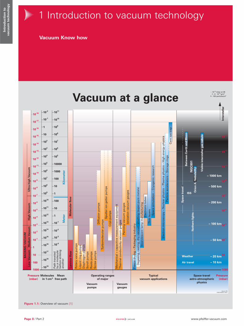
Figure 1.1: Overview of vacuum [1]
www.pfeiffer-vacuum.com
2 Vacuum Technology and Know how / Introduction to vacuum technology
Part 2 / Page 9
Intr
od
uct
ion
to
vacu
um
tec
hn
olo
gy
1.1 General
1.1.1 Vacuum – DefinitionA vacuum is defined colloquially as the state encountered in a room at pressures below atmospheric pressure. These pressures can be generated by gases or vapors that are evenly distributed over the room.
The standard definition of vacuum is “the state of a gas at which its pressure in a vessel and therefore its particle density is lower than that of the ambient surrounding atmosphere or in which the pressure of the gas is lower than 300 mbar, i. e. lower than the pressure of the atmosphere on the Earth’s surface.“ [2]
1.1.2 Overview of vacuumThe significance of the 300 mbar specified in the standard becomes apparent when the barometric formula is considered. Atmospheric pressure sinks with increasing altitude due to the decreasing weight of the column of air over a certain area.
Formula 1-1: Barometric formula
ph Atmospheric pressure at height hp0 Atmospheric pressure at sea level = 1,013.25 mbar or 101,325 Pag Acceleration of gravity = 9.81 m s-2
�0 Density of air at sea level at 0 °C = 1.293 kg m-3
If for the purposes of simplification we assume that the density of the air, the acceleration of gravity and atmospheric pressure at sea level are constant, we obtain by summarizing:
Formula 1-2: Numerical barometric formula
If ph = p0 /2 and the equation is solved for h, the result is the half altitude value h1/2 = 5,548 m. In other words: atmospheric pressure is halved every 5,548 km.
If the height value in the formula is substituted with the height of Mount Everest, we obtain a pressure of 335 mbar or, expressed in the formal SI unit, 33,500 Pa or 335 hPa. This explains the 300 mbar given in the standard as the lowest atmospheric pressure present on the Earth’s surface.
In this book we will give pressures in the SI unit Pa supplemented by the prefix “hecto” in order to correlate the standard-compliant SI unit with the mbar numerical values commonly used in central Europe.
At the cruising altitude of a passenger jet of approxi-mately 10,000 m above the surface of the Earth, atmo-spheric pressure has already decreased to 290 hPa. Weather balloons rise to a height of up to 30 km where the pressure is 24 hPa. Polar-orbiting weather satellites fly along a polar, sun-synchronous orbit at an altitude of about 800 km. The pressure here has already fallen to approximately 10-6 hPa. The greater the distance from a planet, a sun or a sun system, the lower the pressure becomes. The lowest known pressures are found in inter-stellar space.
In a range of technical applications, the pressure is not indicated as absolute but as relative to atmospheric pressure. The pressure range below atmospheric pressure is indicated as a negative number or a percentage. Examples of this are manometers, pressure reducers on gas cylinders or uses for vacuum lifting gear or vacuum transport systems.
Different types of vacuum pumps are used on Earth to generate a vacuum. An overview of the working ranges of the most important types of vacuum pump and vacuum instruments is given in Figure 1.1: Overview of vacuum [1].
1.2 Fundamentals1.2.1 Definition of vacuum Pressure is defined as the ratio of force acting perpen-dicular and uniformly distributed per unit area.
Formula 1-3: Definition of pressure
p Pressure [Pa]F Force [N]; 1 N = 1 kg m s -2
A Area [m2]
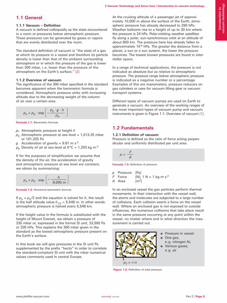
In an enclosed vessel the gas particles perform thermal movements. In their interaction with the vessel wall, the atoms and molecules are subjected to a large number of collisions. Each collision exerts a force on the vessel wall. Where an enclosed gas is not exposed to outside influences, the numerous collisions that take place result in the same pressure occurring at any point within the vessel, no matter where and in what direction the mea-surement is carried out.
Figure 1.2: Definition of total pressure
�0 · g · h
p0ph = p0 · exp
h
8,005 mph = p0 · exp
F
Ap =
Pressure in vessel One gas,
e. g. nitrogen N2
Various gases, e. g. air
pT = F / A
www.pfeiffer-vacuum.comPage 10 / Part 2
2 Vacuum Technology and Know how / Introduction to vacuum technologyIn
trod
uct
ion
to
vacu
um
tec
hn
olo
gy
Gas type Chem. Formula
Volume % Partial pressure [hPa]
Nitrogen N2 78.09 780.9
Oxygen O2 20.95 209.5
Water vapor H2O < 2.3 < 23.3
Argon Ar 9.3 . 10-1 9.3
Carbon dioxide CO2 3.0 . 10-2 3.0 . 10-1
Neon Ne 1.8 . 10-3 1.8 . 10-2
Hydrogen H2 < 1 . 10-3 < 1 . 10-2
Helium He 5.0 . 10-4 5.0 . 10-3
Methane CH4 2.0 . 10-4 2.0 . 10-3
Krypton Kr 1.1 . 10-4 1.1 . 10-3
Carbon monoxide CO < 1,6 . 10-5 < 1,6 . 10-4
Xenon Xe 9.0 . 10-6 9.0 . 10-5
Nitrous oxide N2O 5.0 . 10-6 5.0 . 10-5
Ammonia NH3 2.6 . 10-6 2.6 . 10-5
Ozone O3 2.0 . 10-6 2.0 . 10-5
Hydrogen peroxide H2O2 4.0 . 10-8 4.0 . 10-7
Iodine I2 3.5 . 10-9 3.5 . 10-8
Radon Rn 7.0 . 10-18 7.0 . 10-17
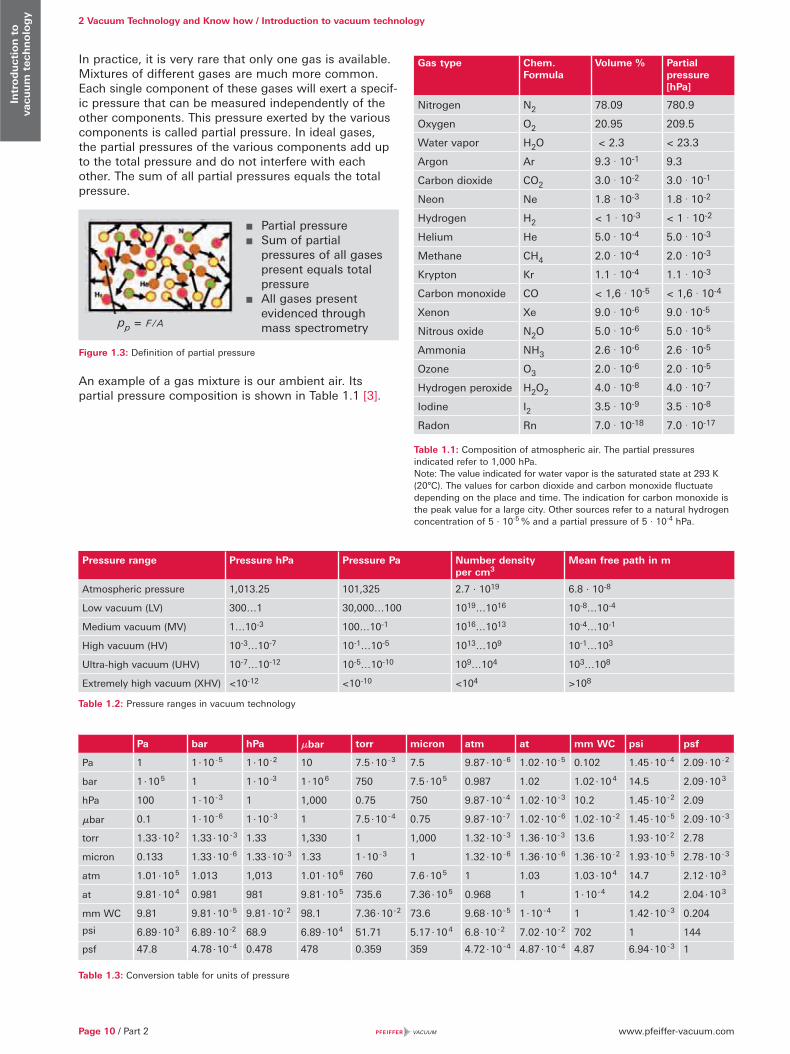
Table 1.1: Composition of atmospheric air. The partial pressures indicated refer to 1,000 hPa.Note: The value indicated for water vapor is the saturated state at 293 K (20°C). The values for carbon dioxide and carbon monoxide fluctuate depending on the place and time. The indication for carbon monoxide is the peak value for a large city. Other sources refer to a natural hydrogen concentration of 5 · 10-5 % and a partial pressure of 5 · 10-4 hPa.
In practice, it is very rare that only one gas is available. Mixtures of different gases are much more common. Each single component of these gases will exert a specif-ic pressure that can be measured independently of the other components. This pressure exerted by the various components is called partial pressure. In ideal gases, the partial pressures of the various components add up to the total pressure and do not interfere with each other. The sum of all partial pressures equals the total pressure.
Figure 1.3: Definition of partial pressure
An example of a gas mixture is our ambient air. Its partial pressure composition is shown in Table 1.1 [3].
Partial pressure Sum of partial
pressures of all gases present equals total pressure
All gases present evidenced through mass spectrometrypp = F / A
Pressure range Pressure hPa Pressure Pa Number densityper cm3
Mean free path in m
Atmospheric pressure 1,013.25 101,325 2.7 · 1019 6.8 · 10-8
Low vacuum (LV) 300…1 30,000…100 1019…1016 10-8…10-4
Medium vacuum (MV) 1…10-3 100…10-1 1016…1013 10-4…10-1
High vacuum (HV) 10-3…10-7 10-1…10-5 1013…109 10-1…103
Ultra-high vacuum (UHV) 10-7…10-12 10-5…10-10 109…104 103…108
Extremely high vacuum (XHV) <10-12 <10-10 <104 >108
Table 1.2: Pressure ranges in vacuum technology
Pa bar hPa �bar torr micron atm at mm WC psi psf
Pa 1 1 · 10 - 5 1 · 10 - 2 10 7.5 · 10 - 3 7.5 9.87 · 10 - 6 1.02 · 10 - 5 0.102 1.45 · 10 - 4 2.09 · 10 - 2
bar 1 · 10 5 1 1 · 10 -3 1 · 10 6 750 7.5 · 10 5 0.987 1.02 1.02 · 10 4 14.5 2.09 · 10 3
hPa 100 1 · 10 - 3 1 1,000 0.75 750 9.87 · 10 - 4 1.02 · 10 - 3 10.2 1.45 · 10 - 2 2.09
�bar 0.1 1 · 10 - 6 1 · 10 - 3 1 7.5 · 10 - 4 0.75 9.87 · 10 - 7 1.02 · 10 - 6 1.02 · 10 - 2 1.45 · 10 - 5 2.09 · 10 - 3
torr 1.33 · 10 2 1.33 · 10 - 3 1.33 1,330 1 1,000 1.32 · 10 - 3 1.36 · 10 - 3 13.6 1.93 · 10 - 2 2.78
micron 0.133 1.33 · 10 - 6 1.33 · 10 - 3 1.33 1 · 10 - 3 1 1.32 · 10 - 6 1.36 · 10 - 6 1.36 · 10 - 2 1.93 · 10 - 5 2.78 · 10 - 3
atm 1.01 · 10 5 1.013 1,013 1.01 · 10 6 760 7.6 · 10 5 1 1.03 1.03 · 10 4 14.7 2.12 · 10 3
at 9.81 · 10 4 0.981 981 9.81 · 10 5 735.6 7.36 · 10 5 0.968 1 1 · 10 - 4 14.2 2.04 · 10 3
mm WC 9.81 9.81 · 10 - 5 9.81 · 10- 2 98.1 7.36 · 10 - 2 73.6 9.68 · 10 - 5 1 · 10 - 4 1 1.42 · 10 - 3 0.204
psi 6.89 · 10 3 6.89 · 10 -2 68.9 6.89 · 10 4 51.71 5.17 · 10 4 6.8 · 10 - 2 7.02 · 10 - 2 702 1 144
psf 47.8 4.78 · 10 - 4 0.478 478 0.359 359 4.72 · 10 - 4 4.87 · 10 - 4 4.87 6.94 · 10 - 3 1
Table 1.3: Conversion table for units of pressure
www.pfeiffer-vacuum.com
2 Vacuum Technology and Know how / Introduction to vacuum technology
Part 2 / Page 11
Intr
od
uct
ion
to
vacu
um
tec
hn
olo
gy
In space, depending on the proximity to galaxies, pres-sures of under 10-18 hPa prevail. On Earth, technically generated pressures of less than 10-16 hPa have been reported. The range of atmospheric pressure down to 10-16 hPa covers 19 decimal powers. Specifically adapted types of vacuum generation and measurement for the pressure range result in subdivisions of the various pres-sure ranges as shown in Table 1.2.
The unit for measuring pressure is the pascal. This unit was named after the French mathematician, physicist, writer and philosopher Blaise Pascal (1623 – 1662). According to Formula 1-3, the SI unit pascal is composed of Pa = N m-2. The units mbar, torr and the units shown in Table 1.3 are common in practical use.
Additional units and their conversion units can be found in our eVacuum app.
1.2.2 General gas equationEach material consists of atoms or molecules. By defini-tion, the amount of substance is indicated in moles. One mole of a material contains 6.022 · 1023 constituent particles (Avogadro constant. This is not a number but a physical magnitude with the unit mol-1). 1 mole is defined as the amount of substance of a system which consists of the same number of particles as the number of atoms contained in exactly 12 g of carbon of the nuclide 12C.
Under normal conditions, i.e. a pressure of 101.325 Pa and a temperature of 273.15 K (equals 0°C), one mole of an ideal gas fills a volume of 22.414 liters.
As early as 1664, Robert Boyle studied the influence of pressure on a given amount of air. The results confirmed by Mariotte in experiments are summarized in the Boyle-Mariotte law:
Formula 1-4: Boyle-Mariotte law [4]
Expressed in words the Boyle-Mariotte law states that the volume of a given quantity of gas at a constant temperature is inversely proportional to the pressure – the product of the pressure and volume is constant.
Over a hundred years later, the temperature dependence of the volume of a quantity of gas was also identified: the volume of a given quantity of gas at a constant pres-sure is directly proportional to the absolute temperature or
Formula 1-5: Gay-Lussac’s law
Subjecting a given quantity of gas successively to a change in pressure and a change in temperature results in
This still applies for a given quantity of gas. The volume of gas at a given temperature and a given pressure is proportional to the quantity of material �. We can therefore write:
The quantity of material is determined by weighing. We can express the quantity of gas by the ratio of mass divided by the molar mass. The constant const. refers here to 1 mole of the gas in question, and it is referred to as the gas constant R. As a result, the state of an ideal gas can be described as follows as a function of pressure, temperature and volume:
Formula 1-6: General equation of state for ideal gases [5]
p Pressure [Pa]V Volume [m3]m Mass [kg]M Molar mass [kg kmol-1]R General gas constant [kJ kmol-1 K-1]T Absolute temperature [K]
The amount of substance � can also be indicated as the number of molecules in relation to the Avogadro constant.
Formula 1-7: Equation of state for ideal gases I
N Number of particles NA Avogadro constant = 6.022 · 1023 [mol-1]k Boltzmann constant = 1.381 · 10-23 [J K-1]
If both sides of the equation are now divided by the volume, then we obtain
Formula 1-8: Equation of state for ideal gases II
n Particle number density [m-3]
p · V = const.
V = const. · T
p · V
T= const.
p · V
T= � · const.
p · V = · R · Tm
M
p · V = · R · T = N · k · T N
NA
where k =R
NA
p = n · k · T
www.pfeiffer-vacuum.comPage 12 / Part 2
2 Vacuum Technology and Know how / Introduction to vacuum technologyIn
trod
uct
ion
to
vacu
um
tec
hn
olo
gy
1.2.3 Molecular number densityAs can be seen from Formula 1-7 and Formula 1-8 pressure is proportional to particle number density. Due to the high number of particles per unit of volume at standard conditions, it follows that at a pressure of 10-12 hPa, for example, 26,500 molecules per cm³ will still be present. This is why it is not possible to speak of a void, or nothingness, even under ultra-high vacuum.
In space it is increasingly ineffective at extremely low pressures to express pressure in the unit Pascal, e. g. less than10-18 hPa. These pressure ranges can be better expressed by the particle number density, e. g. < 104 molecules per cubic meter in interplanetary space.
1.2.4 Thermal velocityGas molecules enclosed in a vessel collide entirely ran-domly with each other. Energy and impulses are trans-mitted in the process. As a result of this transmission, a distribution of velocity and/or kinetic energy occurs. The velocity distribution corresponds to a bell curve (Maxwell-Boltzmann distribution) having its peak at the most probable velocity.
Formula 1-9: Most probable speed [6]
The mean thermal velocity is
Formula 1-10: Mean speed [7]
The following table shows the mean thermal velocity for selected gases at a temperature of 20°C.
Gas Chemical Symbol
Molar Mass[g mol-1]
Mean Velocity [m s-1]
Mach Number
Hydrogen H2 2 1,754 5.3
Helium He 4 1,245 3.7
Water vapor H2O 18 585 1.8
Nitrogen N2 28 470 1.4
Air 29 464 1.4
Argon Ar 40 394 1.2
Carbon dioxide CO2 44 375 1.1
Table 1.4: Molar masses and mean thermal velocities of various gases [8]
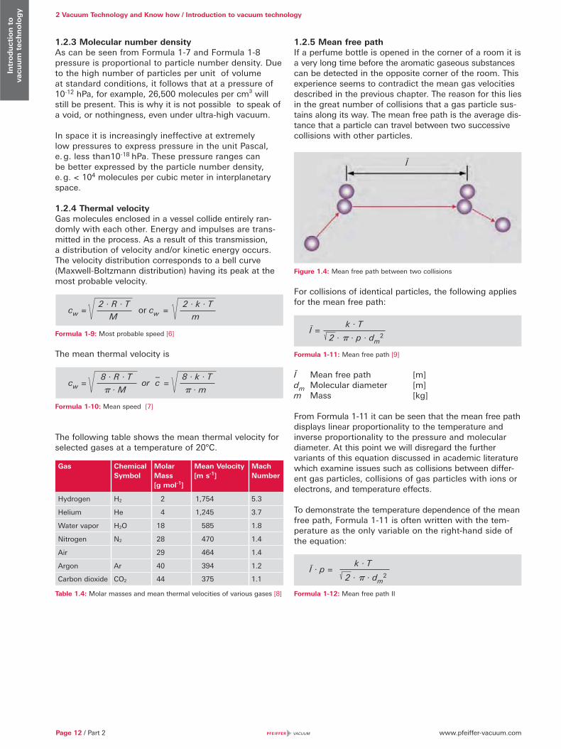
1.2.5 Mean free pathIf a perfume bottle is opened in the corner of a room it is a very long time before the aromatic gaseous substances can be detected in the opposite corner of the room. This experience seems to contradict the mean gas velocities described in the previous chapter. The reason for this lies in the great number of collisions that a gas particle sus-tains along its way. The mean free path is the average dis-tance that a particle can travel between two successive collisions with other particles.
Figure 1.4: Mean free path between two collisions
For collisions of identical particles, the following applies for the mean free path:
Formula 1-11: Mean fr ee path [9]
Ī Mean free path [m]dm Molecular diameter [m]m Mass [kg]
From Formula 1-11 it can be seen that the mean free path displays linear proportionality to the temperature and inverse proportionality to the pressure and molecular diameter. At this point we will disregard the further variants of this equation discussed in academic literature which examine issues such as collisions between differ-ent gas particles, collisions of gas particles with ions or electrons, and temperature effects.
To demonstrate the temperature dependence of the mean free path, Formula 1-11 is often written with the tem-perature as the only variable on the right-hand side of the equation:
Formula 1-12: Mean free path II
cw = 2 · R · T
Mor cw =
2 · k · T
m
cw = 8 · R · T
� · Mor c
– =
8 · k · T
� · m
Ī
Ī =
k · T
2 · � · p · dm2
Ī · p =
k · T
2 · � · dm2
www.pfeiffer-vacuum.com
2 Vacuum Technology and Know how / Introduction to vacuum technology
Part 2 / Page 13
Intr
od
uct
ion
to
vacu
um
tec
hn
olo
gy
Table 1.5 shows the Ī · p values for a number of selected gases at 0°C.
Gas Chemical Symbol
Ī · p[m hPa]
Ī · p[m Pa]
Hydrogen H2 11.5 . 10-5 11.5 . 10-3
Nitrogen N2 5.9 . 10-5 5.9 . 10-3
Oxygen O2 6.5 . 10-5 6.5 . 10-3
Helium He 17.5 . 10-5 17.5 . 10-3
Neon Ne 12.7 . 10-5 12.7 . 10-3
Argon Ar 6.4 . 10-5 6.4 . 10-3
Air 6.7 . 10-5 6.7 . 10-3
Krypton Kr 4.9 . 10-5 4.9 . 10-3
Xenon Xe 3.6 . 10-5 3.6 . 10-3
Mercury Hg 3.1 . 10-5 3.1 . 10-3
Water vapor H2O 6.8 . 10-5 6.8 . 10-3
Carbon monoxide CO 6.0 . 10-5 6.0 . 10-3
Carbon dioxide CO2 4.0 . 10-5 4.0 . 10-3
Hydrogen chloride HCl 3.3 . 10-5 3.3 . 10-3
Ammonia NH3 3.2 . 10-5 3.2 . 10-3
Chlorine Cl2 2.1 . 10-5 2.1 . 10-3
Table 1.5: Mean free path of selected gases at 273.15K [10]
Using the values from Table 1.5 we now estimate the mean free path of a nitrogen molecule at various pressures:
Pressure [Pa] Pressure [hPa] Mean free path [m]
1 . 105 1 . 103 5.9 . 10-8
1 . 104 1 . 102 5.9 . 10-7
1 . 103 1 . 101 5.9 . 10-6
1 . 102 1 . 100 5.9 . 10-5
1 . 101 1 . 10-1 5.9 . 10-4
1 . 100 1 . 10-2 5.9 . 10-3
1 . 10-1 1 . 10-3 5.9 . 10-2
1 . 10-2 1 . 10-4 5.9 . 10-1
1 . 10-3 1 . 10-5 5.9 . 100
1 . 10-4 1 . 10-6 5.9 . 101
1 . 10-5 1 . 10-7 5.9 . 102
1 . 10-6 1 . 10-8 5.9 . 103
1 . 10-7 1 . 10-9 5.9 . 104
1 . 10-8 1 . 10-10 5.9 . 105
1 . 10-9 1 . 10-11 5.9 . 106
1 . 10-10 1 . 10-12 5.9 . 107
Table 1.6: Mean free path of a nitrogen molecule at 273.15K (0°C)
At atmospheric pressure a nitrogen molecule therefore travels a distance of 59 nm between two collisions, while at ultra-high vacuum at pressures below 10-8 hPa it travels a distance of several kilometers.
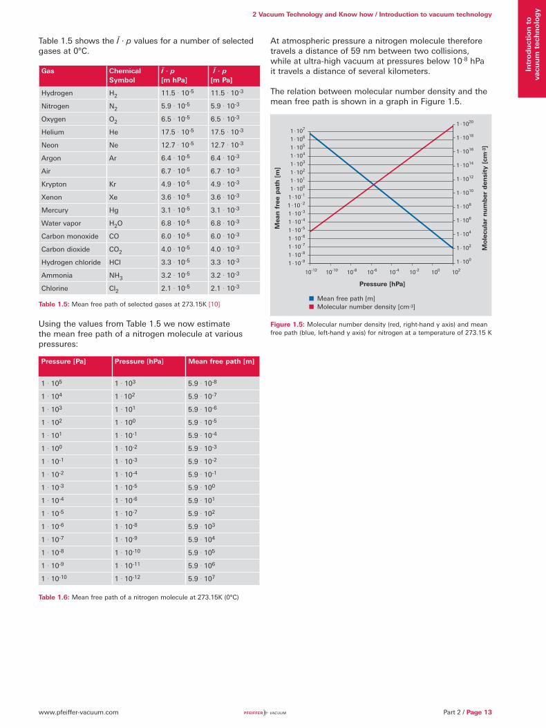
The relation between molecular number density and the mean free path is shown in a graph in Figure 1.5.
Figure 1.5: Molecular number density (red, right-hand y axis) and mean free path (blue, left-hand y axis) for nitrogen at a temperature of 273.15 K
1 · 107
1 · 106
1 · 105
1 · 104
1 · 103
1 · 102
1 · 101
1 · 100
1 · 10- 1
1 · 10 - 2
1 · 10- 3
1 · 10- 4
1 · 10- 5
1 · 10- 6
1 · 10- 7
1 · 10- 8
1 · 10- 9
1 · 1020
1 · 1018
1 · 1016
1 · 1014
1 · 1012
1 · 1010
1 · 108
1 · 106
1 · 104
1 · 102
1 · 100
Mea
n f
ree
pat
h [
m]
Mole
cula
r n
um
ber
den
sity
[cm
-3]
10-12 10-10 10-8 10-6 10-4 10-2 100 102
Pressure [hPa]
Mean free path [m] Molecular number density [cm-3]
www.pfeiffer-vacuum.comPage 14 / Part 2
2 Vacuum Technology and Know how / Introduction to vacuum technologyIn
trod
uct
ion
to
vacu
um
tec
hn
olo
gy
1.2.6 Types of flowThe ratio of the mean free path to the flow channel diameter can be used to describe types of flow. This ratio is referred to as the Knudsen number:
Formula 1-13: Knudsen number
Ī Mean free path [m]d Diameter of flow channel [m]Kn Knudsen number dimensionless
The value of the Knudsen number characterizes the type of gas flow and assigns it to a particular pressure range. Table 1.7 gives an overview of the various types of flow in vacuum technology and their significant characteriza-tion parameters.
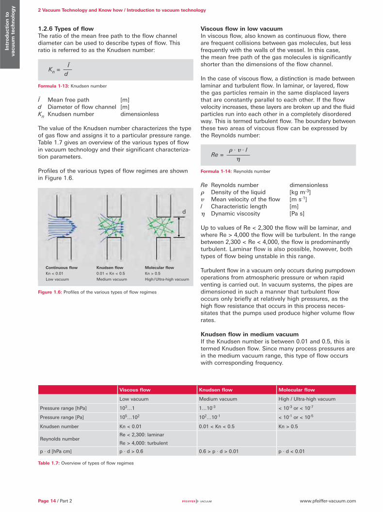
Profiles of the various types of flow regimes are shown in Figure 1.6.
Fig ure 1.6: Profiles of the various types of flow regimes
Viscous flow in low vacuumIn viscous flow, also known as continuous flow, there are frequent collisions between gas molecules, but less frequently with the walls of the vessel. In this case, the mean free path of the gas molecules is significantly shorter than the dimensions of the flow channel.
In the case of viscous flow, a distinction is made between laminar and turbulent flow. In laminar, or layered, flow the gas particles remain in the same displaced layers that are constantly parallel to each other. If the flow velocity increases, these layers are broken up and the fluid particles run into each other in a completely disordered way. This is termed turbulent flow. The boundary between these two areas of viscous flow can be expressed by the Reynolds number:
Formula 1-14: Reynolds number
Re Reynolds number dimensionless� Density of the liquid [kg m-3]� Mean velocity of the flow [m s-1]l Characteristic length [m]� Dynamic viscosity [Pa s]
Up to values of Re < 2,300 the flow will be laminar, and where Re > 4,000 the flow will be turbulent. In the range between 2,300 < Re < 4,000, the flow is predominantly turbulent. Laminar flow is also possible, however, both types of flow being unstable in this range.
Turbulent flow in a vacuum only occurs during pumpdown operations from atmospheric pressure or when rapid venting is carried out. In vacuum systems, the pipes are dimensioned in such a manner that turbulent flow occurs only briefly at relatively high pressures, as the high flow resistance that occurs in this process neces-sitates that the pumps used produce higher volume flow rates.
Knudsen flow in medium vacuumIf the Knudsen number is between 0.01 and 0.5, this is termed Knudsen flow. Since many process pressures are in the medium vacuum range, this type of flow occurs with corresponding frequency.
Viscous flow Knudsen flow Molecular flow
Low vacuum Medium vacuum High / Ultra-high vacuum
Pressure range [hPa] 103…1 1…10-3 < 10-3 or < 10-7
Pressure range [Pa] 105…102 102…10-1 < 10-1 or < 10-5
Knudsen number Kn < 0.01 0.01 < Kn < 0.5 Kn > 0.5
Reynolds numberRe < 2,300: laminar
Re > 4,000: turbulent
p · d [hPa cm] p · d > 0.6 0.6 > p · d > 0.01 p · d < 0.01
Table 1.7: Overview of types of flow regimes
Continuous flow
Kn < 0.01
Low vacuum
Knudsen flow
0.01 < Kn < 0.5
Medium vacuum
Molecular flow
Kn > 0.5
High / Ultra-high vacuum
Kn =
Ī
d
Re =
� · � · l
�
d

www.pfeiffer-vacuum.com
2 Vacuum Technology and Know how / Introduction to vacuum technology
Part 2 / Page 15
Intr
od
uct
ion
to
vacu
um
tec
hn
olo
gy
Molecular flow in high vacuum and ultra-high vacuumAt Knudsen numbers of Kn > 0.5 molecular interaction virtually no longer occurs. What prevails is molecular flow. In this case, the mean free path is significantly greater than the diameter of the flow channel. In molecular flow, the product of pressure and component diameter is approximately ≤ 1.3 · 10-2 hPa cm.
A graph showing an overview of flow ranges as a func-tion of the product of pressure and component diameter is displayed in Figure 1.7.
Figure 1.7: Flow ranges in vacuum as a function of p · d
This graph clearly shows that the classification, also found in Table 1.7, into vacuum ranges purely according to pressure is an inadmissible simplification. Since this classification is still in common usage, however, it is cited here.
1.2.7 pV throughputDividing the general gas equation (Formula 1-6) by time t obtains the gas flow
Formula 1-15: pV throughput
qpV pV throughput [Pa m3 s-1]
As can be seen from the right-hand side of the equation, a constant mass flow is displaced at constant tempera-ture T. This is also referred to as pV flow or gas through-put. Throughput is the gas flow rate transported by a vacuum pump.
Formula 1-16: Throughput of a vacuum pump
Dividing the through put by the inlet pressure obtains a volume flow rate, the pumping speed of a vacuum pump:
Formula 1-17: Volume flow rate, or pumping speed, of a vacuum pump
A conversion table for various units of throughput is given in Table 1.8.
Additional units and their convers ion can be found in our eVacuum app.
Pressure p
Pip
e d
iam
eter
d
hPa
100cm
10
1
10 -5 10 -4 10 -3 10 -2 10 -1 10 0 10 1 10 2 10 3
Viscous
Molecular
qpV = p · V
t=
m · R · T
M · t
qpV = S · p = · p
S =
dV
dt
dV
dt
Pa m3 / s = W mbar l / s torr l / s atm cm3 / s lusec sccm slm mol / s
Pa m3/s 1 10 7.5 9.87 7.5 · 103 592 0.592 4.41 · 10-4
mbar l / s 0.1 1 0.75 0.987 750 59.2 5.92 · 10-2 4.41 · 10-5
torr l / s 0.133 1.33 1 1.32 1,000 78.9 7.89 · 10-2 5.85 · 10-5
atm cm3 / s 0.101 1.01 0.76 1 760 59.8 5.98 · 10-2 4.45 · 10-5
lusec 1.33 · 10-4 1.33 · 10-3 10-3 1.32 · 10-3 1 7.89 · 10-2 7.89 · 10-5 5.86 · 10-8
sccm 1.69 · 10-3 1.69 · 10-2 1.27 · 10-2 1.67 · 10-2 12.7 1 10-3 7.45 · 10-7
slm 1.69 16.9 12.7 16.7 1.27 · 104 1,000 1 7.45 · 10-4
mol / s 2.27 · 103 2.27 · 104 1.7 · 104 2.24 · 104 1.7 · 107 1.34 · 106 1.34 · 103 1
Table 1.8: Conversion table for units of throughput
Transition regime
www.pfeiffer-vacuum.comPage 16 / Part 2
2 Vacuum Technology and Know how / Introduction to vacuum technologyIn
trod
uct
ion
to
vacu
um
tec
hn
olo
gy
1.2.8 ConductanceGenerally speaking, vacuum chambers are connected to a vacuum pump via piping. Flow resistance occurs as a result of external friction between gas molecules and the wall surface and internal friction between the gas molecules themselves (viscosity). This flow resistance manifests itself in the form of pressure differences and volume flow rate, or pumping speed, losses. In vacuum technology, it is customary to use the reciprocal, the conductivity of piping L or C (conductance) instead of flow resistance W. The conductivity has the dimension of a volume flow rate and is normally expressed in [l s-1] or [m3 h-1].
Gas flowing through piping produces a pressure differential � p at the ends of the piping. The following equation applies:
Formula 1-18: Definition of conductance
This principle is formally analogous to Ohm’s law of electrotechnology:
Formula 1-19: Ohm’s law
In a formal comparison of Formula 1-18 with Formula 1-19 qpV represents flow I, C the reciprocal of resistance 1/R and � p the voltage U. If the components are con-nected in parallel, the individual conductivities are added:
Formula 1-20
and if connected in series, the resistances, i. e. the reciprocals, are added together:
Formula 1-21: Series connection conductivities
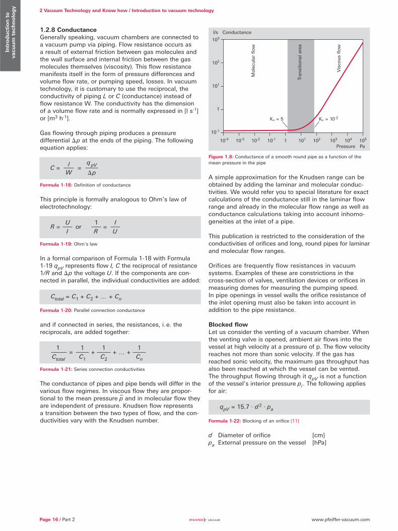
The conductance of pipes and pipe bends will differ in the various flow regimes. In viscous flow they are propor-tional to the mean pressure p
– and in molecular flow they
are independent of pressure. Knudsen flow represents a transition between the two types of flow, and the con-ductivities vary with the Knudsen number.
Figure 1.8: Conductance of a smooth round pipe as a function of the mean pressure in the pipe
A simple approximation for the Knudsen range can be obtained by adding the laminar and molecular conduc-tivities. We would refer you to special literature for exact calculations of the conductance still in the laminar flow range and already in the molecular flow range as well as conductance calculations taking into account inhomo-geneities at the inlet of a pipe.
This publication is restricted to the consideration of the conductivities of orifices and long, round pipes for laminar and molecular flow ranges.
Orifices are frequently flow resistances in vacuum systems. Examples of these are constrictions in the cross-section of valves, ventilation devices or orifices in measuring domes for measuring the pumping speed. In pipe openings in vessel walls the orifice resistance of the inlet opening must also be taken into account in addition to the pipe resistance.
Blocked flowLet us consider the venting of a vacuum chamber. When the venting valve is opened, ambient air flows into the vessel at high velocity at a pressure of p. The flow velocity reaches not more than sonic velocity. If the gas has reached sonic velocity, the maximum gas throughput has also been reached at which the vessel can be vented. The throughput flowing through it qpV is not a function of the vessel’s interior pressure pi . The following applies for air:
Formula 1-22: Blocking of an orifice [11]
d Diameter of orifice [cm]pa External pressure on the vessel [hPa]
C = l
W=
q pV
� p
R = orU
I
1
R
I
U=
=1
Ctotal
1
C1
1
C2
1
Cn
+ + … +
Ctotal = C1 + C2 + … + Cn
qpV = 15.7 · d 2 · pa
103
102
101
1
10-1
Mo
lecu
lar
flow
Tran
siti
on
al a
rea
Vis
cou
s fl
ow
Kn = 5 Kn = 10-2
10-4 10-3 10-2 10-1 1 101 102 103 104 105
l/s Conductance
Pressure Pa
: Parallel connection conductance

www.pfeiffer-vacuum.com
2 Vacuum Technology and Know how / Introduction to vacuum technology
Part 2 / Page 17
Intr
od
uct
ion
to
vacu
um
tec
hn
olo
gy
Gas dynamic flowIf the pressure in the vessel now rises beyond a critical pressure, gas flow is reduced and we can use gas dynamic laws according to Bernoulli and Poiseuille to calculate it. The immersive gas flow qpV and the conductance are dependent on
Narrowest cross-section of the orifice External pressure on the vessel Internal pressure in the vessel Universal gas constant Absolute temperature Molar mass Adiabatic exponent (= ratio of specific or molar
heat capacities at constant pressure cp or constant volume cV ) [12]
Molecular flow [13] If an orifice connects two vessels in which molecular flow conditions exist (i.e. if the mean free path is considerably greater than the diameter of the vessel), the following will apply for the displaced gas quantity qpV per unit of time
Formula 1-23: Orifice flow
A Cross-section of orifice [cm2]c– Mean thermal velocity [m s-1]
According to Formula 1-23 the following applies for the orifice conductivity
Formula 1-24: Orifice conductivity
For air with a temperature of 293 K we obtain
Formula 1-25: Orifice conductivity for air
A Cross-section of orifice [cm2]C Conductivity [l s-1]
This formula can be used to determine the maximum possible pumping speed of a vacuum pump with an inlet port A. The maximum pumping speed of a pump under molecular flow conditions is therefore determined by the inlet port.
Let us now consider specific pipe conductivities. In the case of laminar flow, the conductivity of a pipe is proportional to the mean pressure:
Formula 1-26: Conductance of a pipe in laminar flow
For air at 20°C we obtain
Formula 1-27: Conductance of a pipe in laminar flow for air
l Length of pipe [cm]d Diameter of pipe [cm]p– Pressure [Pa]
C Conductivity [l s-1]
In the molecular flow regime, conductance is constant and is not a function of pressure. It can be considered to be the product of the orifice conductivity of the pipe opening Cpipe, mol and passage probability Ppipe, mol through a component:
Formula 1-28: Molecular pipe flow
The mean probability Ppipe, mol can be calculated with a computer program for different pipe profiles, bends or valves using a Monte Carlo simulation. In this connection, the trajectories of individual gas molecules through the component can be tracked on the basis of wall collisions.
The following applies for long round pipes:
Formula 1-29: Passage probability for long round pipes
If we multiply this value by the orifice conductivity (Formula 1-24), we obtain
Formula 1-30: Molecular pipe conductivity
For air at 20°C we obtain
Formula 1-31: Molecular pipe conductivity
l Length of pipe [cm]d Diameter of pipe [cm]C Conductivity [l s-1]
C or, mol = A ·c–
4= A ·
kT2� m0
C or, mol = 11.6 · A
C pipe, lam = · (p1 + p2) = · p–� · d 4
256 · � · l
� · d 4
228 · � · l
C pipe, lam = 1.35 · · p–d4
l
Cpipe, mol = Corifice, mol · Ppipe, mol
C pipe, mol = c– · � · d 3
12 · l
C pipe, lam = 12.1 · d 3
l
Cpipe, mol = 43
dl
·
qpV = A · c–
4· (p1 - p2 )
www.pfeiffer-vacuum.comPage 18 / Part 2
2 Vacuum Technology and Know how / Introduction to vacuum technologyIn
trod
uct
ion
to
vacu
um
tec
hn
olo
gy
1.3 Influences in real vacuum systems
1.3.1 ContaminationVacuum chambers must be clean in order to reach the desired pressure as quickly as possible when they are pumped down. Typical contaminants of vacuum systems include
Residues from the production of the vacuum systems Oil and grease on surfaces, screws and seals
Application-related contaminants Process reaction products, dust and particles
Ambient-related contaminants Condensed vapors, particularly water that is adsorbed on the walls of the vessel.
Consequently, it is necessary to ensure that the compo-nents are as clean as possible when installing vacuum equipment. All components attached in the vacuum chamber must be clean and grease-free. All seals must also be installed dry. If the use of vacuum grease cannot be avoided, it must be used extremely sparingly, if at all, to aid installation but not as a sealant. If high or ultra-high vacuum is to be generated, clean lint-free and powder-free gloves must be worn during the assembly process.
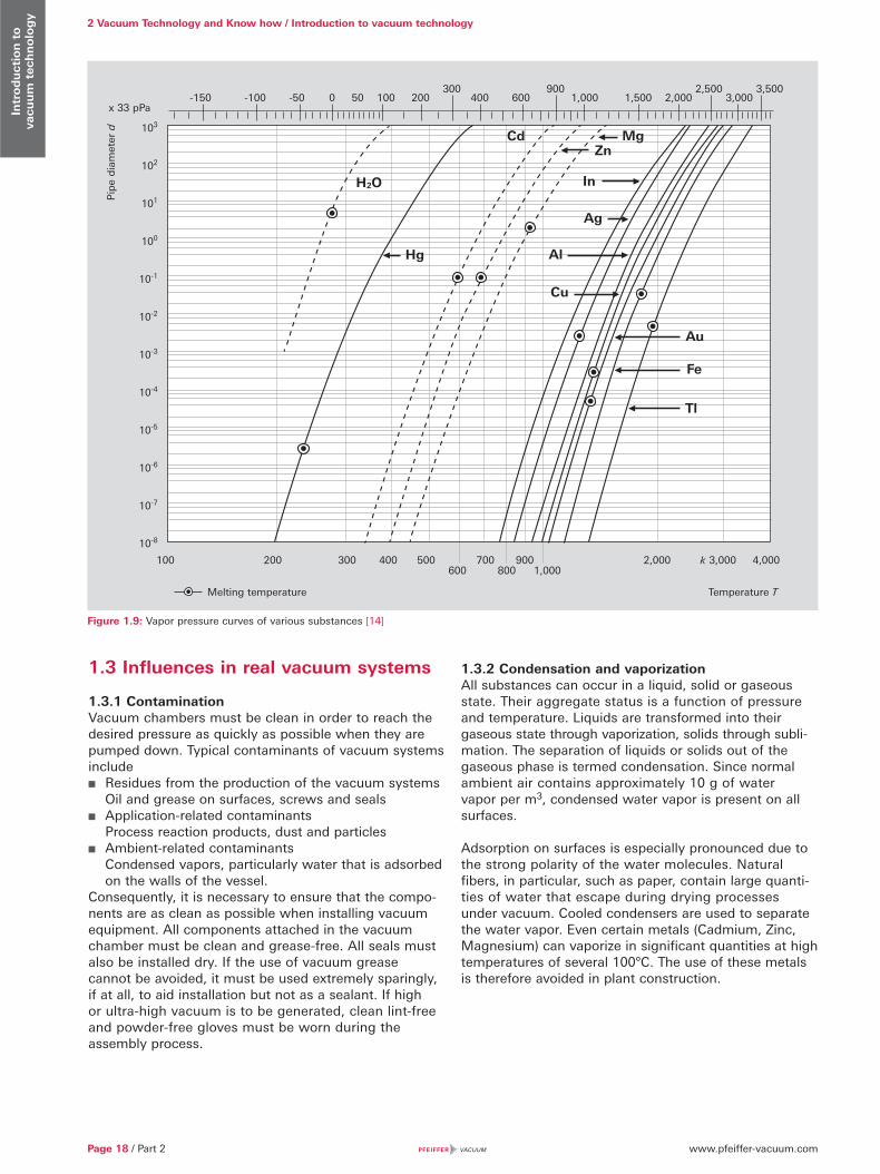
1.3.2 Condensation and vaporizationAll substances can occur in a liquid, solid or gaseous state. Their aggregate status is a function of pressure and temperature. Liquids are transformed into their gaseous state through vaporization, solids through subli-mation. The separation of liquids or solids out of the gaseous phase is termed condensation. Since normal ambient air contains approximately 10 g of water vapor per m3, condensed water vapor is present on all surfaces.
Adsorption on surfaces is especially pronounced due to the strong polarity of the water molecules. Natural fibers, in particular, such as paper, contain large quanti-ties of water that escape during drying processes under vacuum. Cooled condensers are used to separate the water vapor. Even certain metals (Cadmium, Zinc, Magnesium) can vaporize in significant quantities at high temperatures of several 100°C. The use of these metals is therefore avoided in plant construction.
Melting temperature Temperature T
H2O
Hg
Cd MgZn
In
Ag
Al
Cu
Au
Fe
Tl
Pip
e d
iam
eter
d-150 -100 -50 0 50 100 200
300 400 600
900 1,000 1,500 2,000
2,500 3,000
3,500
103
102
101
100
10-1
10-2
10-3
10-4
10-5
10-6
10-7
10-8
x 33 pPa
100 200 300 400 500 600
700 800
9001,000
2,000 k 3,000 4,000
Figure 1.9: Vapor pressure curves of various substances [14]
www.pfeiffer-vacuum.com
2 Vacuum Technology and Know how / Introduction to vacuum technology
Part 2 / Page 19
Intr
od
uct
ion
to
vacu
um
tec
hn
olo
gy
1.3.3 Desorption, diffusion, permeation and leaksIn addition to water, other substances such as vacuum pump operating fluids can be adsorbed on surfaces. Substances can also diffuse out of the metal walls, which can be evidenced in the residual gas. In the case of particularly rigorous requirements, stainless steel vessels can be baked out under vacuum, thus driving the majority of the volatile components out of the metal walls.
DesorptionGas molecules, (primarily water) are bound to the interior surfaces of the vacuum chamber through adsorption and absorption, and gradually desorb again under vacuum. The desorption rate of the metal and glass surfaces in the vacuum system produces a gas yield that declines over time as the coverage rate decreases. A good approximation can be obtained by assuming that after a given point in time t > t0 the reduction will occur on a linear basis over time. t0 is typically assumed to be one hour.
The gas yield can thus be described as:
Formula 1-32: Desorption rate
Qdes Desorption rate [Pa m3 s-1]qdes Desorption flow density (area-specific) [Pa m3 s-1 m-2]A Area [m2]t Time [s]
Diffusion with desorptionAt operation below 10-6 hPa desorption of plastic surfaces, particularly the seals, assumes greater significance. Plastics mainly give off the gases that are dissolved in these plastics, which first must diffuse on the surface. Following extended pump downtimes, desorption from plastics can therefore dominate desorption from metal surfaces. Although the surface areas of the seals are relatively small; the decrease in the desorption rate over time occurs more slowly than in the case of metal surfaces. As an approximation it can be assumed that the reduction over time will occur at the square root of the time.
The gas produced from plastic surfaces can thus be described as:
Formula 1-33: Desorption rate from plastics
Qdiff Diffusion rate [Pa m3 s-1]qdiff Diffusion flow density (area-specific) [Pa m3 s-1 m-2]Ad Surface of plastic material in the vessel [m2]t Time [s]
Similar effects also occur at even lower pressures in metals, where hydrogen and carbon escape in the form of CO and CO2, and can be seen in the residual gas spectrum. Formula 1-33 also applies in this regard.
Permeation and leaksSeals, and even metal walls, can be penetrated by small gas molecules, such as helium,through diffusion. Since this process is not a function of time, it results in a sustained increase in the desired ultimate pressure. The permeation gas flow is proportional to the pressure gradient across the wall thickness and a material-depen-dent permeation constant.
Formula 1-34: Permeation
Qperm Diffusion rate [Pa m3 s-1]pa Pressure outside the vessel [Pa]d Wall thickness [m]A Surface of the vessel [m2]kperm Permeation constant [m2 s-1]
Permeation first manifests itself at pressures below 10-8 hPa.
QL describes the leak rate, i.e. a gas flow, which enters the vacuum system through leaks. The leakage rate is defined as the pressure rise over time in a given volume:
Formula 1-35: Leak rate
QL Leakage rate [Pa m3 s-1]
� p Pressure change during measurement period [Pa]V Volume [m3]� t Measurement period [s]
If a vessel is continuously pumped out at a volume flow rate S, an equilibrium pressure peq will be produced if the throughput (Formula 1-16) is equal to the leakage rate QL = S · peq.
A system is considered to be adequately tight if the equilibrium pressure peq is approximately 10 % of the working pressure. If, for example, a working pressure of 10-6 hPa is to be attained and the vacuum pump that is being used has a pumping speed of 100 l s-1, the leakage rate should not be more than s 10-6 Pa m3 s-1.
Leakage rates QL < 10-9 Pa m3 s-1 can usually be easily attained in clean stainless steel vessels.
Qdes = qdes · A ·t0t
Qdiff = qdiff · Ad ·t0t
Qperm = kperm · A ·pa
d
QL =� p · V
� t
www.pfeiffer-vacuum.comPage 20 / Part 2
2 Vacuum Technology and Know how / Introduction to vacuum technologyIn
trod
uct
ion
to
vacu
um
tec
hn
olo
gy
The ultimate pressure achievable after a given period of time t primarily depends upon all of the effects described above and upon the pumping speed of the vacuum pump. The prerequisite is naturally that the ultimate pressure will be high relative to the base pressure of the vacuum pump.
Formula 1-36: Ultimate pressure as a function of time
The various gas flows and the resulting pressures can be calculated for a given pumping timet by using Formula 1-36 and by solving the equations in relation to the time. The achievable ultimate pressure is the sum of these pressures.
1.3.4 Bake-outTo achieve pressures in the ultra-high vacuum range (<10-8 hPa) the following conditions must be met:
The base pressure of the vacuum pump should be a factor of 10 lower than the required ultimate pressure.
The materials used for the vacuum chamber and components must be optimized for minimum outgas-sing and have an appropriate surface finish grade.
Metallic seals (e. g. CF flange connections or Helicoflex seals for ISO flange standards) should be used.
Clean work is a must for ultra-high vacuum, i. e. all parts must be thoroughly cleaned before installation and must be installed with grease-free gloves.
The equipment and high vacuum pump must be baked out.
Leaks must be avoided and eliminated prior to acti-vating the heater. A helium leak detectors or a quadrupole mass spectrometer must be used for this purpose.
Bake-out significantly increases desorption and diffusion rates, and this produces significantly shorter pumping times. As one of the last steps in the manufacturing pro-cess, chambers for UHV use can be annealed at temper-atures of up to 900 °C. Subsequent bake-out temperatures may reach up to 300 °C in tents. Pump manufacturers΄ instructions relating to maximum bake-out temperatures in the high vacuum pump flange normally restrict the maximum temperature during operation to 120 °C. If heat sources are used in the vacuum equipment (e. g. radia-tion heating), then the admissible radiated power must not be exceeded.
The equipment is put into operation after it has been installed. After reaching a pressure of 10-5 hPa the heat-er is switched on. During the heating process, all vacu-um gauges must be operated and degassed at intervals of 10 hours. If stainless steel vessels with an appropriate surface finish grade and metal seals are used, bake-out temperatures of 120°C and heating times of approxi-mately 48 hours are sufficient for advancing into the pressure range of 10- 10 hPa.
Bake-out should be continued until 100 times the expected ultimate pressure is attained. The heaters for the pump and vacuum chamber are then switched off.
After cool-down, the desired ultimate pressure will prob-ably be achieved. At pressures of less than 5 · 10-10 hPa and large interior surface areas, it will be advantageous to use a gas-binding pump (titanium sublimation pump) that pumps the hydrogen escaping from the metals at a high volume flow rate.
1.3.5 Residual gas compositionWhen working in ultra-high vacuum, it can be important to know the composition of the residual gas before starting vacuum processes or in order to monitor and control processes. The percentages of water (m/e = 18) and its fragment OH (m/e = 17) will be large in the case of vacuum chambers that are not clean or well baked. Leaks can be identified by the peaks of nitrogen (m/e = 28) and oxygen (m/e = 32) in the ratio N2/O2 of approx. 4 to 1.
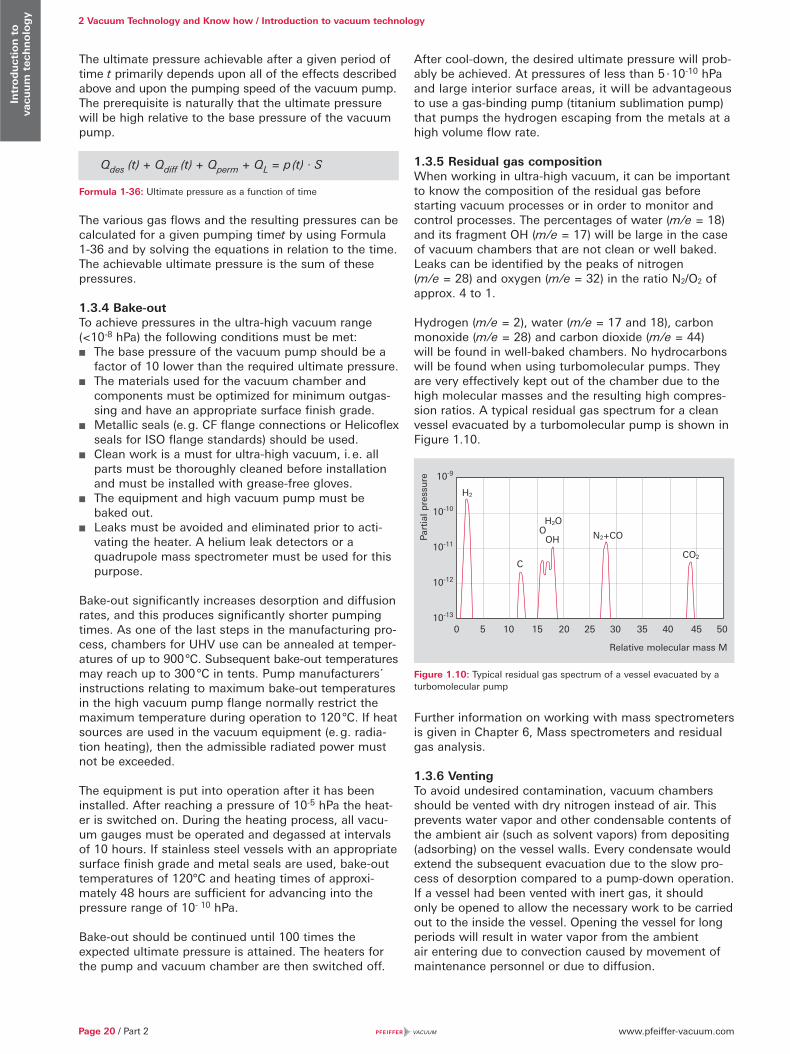
Hydrogen (m/e = 2), water (m/e = 17 and 18), carbon monoxide (m/e = 28) and carbon dioxide (m/e = 44) will be found in well-baked chambers. No hydrocarbons will be found when using turbomolecular pumps. They are very effectively kept out of the chamber due to the high molecular masses and the resulting high compres-sion ratios. A typical residual gas spectrum for a clean vessel evacuated by a turbomolecular pump is shown in Figure 1.10.
Figure 1.10: Typical residual gas spectrum of a vessel evacuated by a turbomolecular pump
Further information on working with mass spectrometers is given in Chapter 6, Mass spectrometers and residual gas analysis.
1.3.6 VentingTo avoid undesired contamination, vacuum chambers should be vented with dry nitrogen instead of air. This prevents water vapor and other condensable contents of the ambient air (such as solvent vapors) from depositing (adsorbing) on the vessel walls. Every condensate would extend the subsequent evacuation due to the slow pro-cess of desorption compared to a pump-down operation. If a vessel had been vented with inert gas, it should only be opened to allow the necessary work to be carried out to the inside the vessel. Opening the vessel for long periods will result in water vapor from the ambient air entering due to convection caused by movement of maintenance personnel or due to diffusion.
Qdes (t) + Qdiff (t) + Qperm + QL = p (t) · S
0 5 10 15 20 25 30 35 40 45 50
10-9
10-10
10-11
10-12
10-13
Relative molecular mass M
Par
tial
pre
ssu
re
H2
C
H2OO
OH N2+CO
CO2

www.pfeiffer-vacuum.com
2 Vacuum Technology and Know how / Introduction to vacuum technology
Part 2 / Page 21
Intr
od
uct
ion
to
vacu
um
tec
hn
olo
gy
www.pfeiffer-vacuum.comPage 22 / Part 2
Bas
ic c
alcu
lati
on
s
2 Basic calculations
2.1 General
This section will discuss simple dimensioning questions: What size pump should I select in order to attain a
specific pressure in a vacuum vessel within a given period of time?
How large should the backing pump be for a high vacuum pump?
What do I need to be aware of when pumping high gas loads?
What is the influence of piping on the effective pumping speed of a vacuum pump?
All of these questions can naturally not be discussed exhaustively in this chapter. Simple examples will be used and the anticipated results estimated. The technical data of the pumps and components that are used must be taken into consideration for the concrete application in question. And special literature [15, 16, 17, 18, 19] can also be useful for dimensioning.
UnitsEvery physical technical parameter consists of a numeric value and a unit. The International System of Units (SI, from the French Système international d'unités) has been adopted worldwide and standards have been defined for the basic values of length (m), mass (kg), time (s), thermodynamic temperature (K), amount of substance (mol), electric current (A) and luminous inten-sity (cd). International regulations concerning the SI system are made by the Bureau International des Poids et Mesures (abbreviated to BIPM) and these are imple-mented nationally by the metrology institutions in the individual countries.
All other values are derived from these basic values. With few exceptions, the formulas that are used in this compendium contain only the physical technical values and no conversion factors whatever. This means that after expressing the values in SI units, the results will also be in SI units. Examples of SI units are 1 Pa = 1 N m-2 = 0.01 hPa for pressure and 1 m3 s-1 = 3.600 m3 h-1. Used largely throughout the following sections are popular non-SI units; however SI units will be used wherever it seems appropriate due to the required conversion. Exclusive use of SI units would avoid many errors and much conversion effort. Unfortunately, this advantage is only very slowly gaining acceptance throughout the world.
2.2 Calculations 2.2.1 Dimensioning a Roots pumping stationVarious preliminary considerations are first required in dimensioning a Roots pumping station.
Compression ratioThe compression ratio K0 of a Roots pump is typically between 5 and 70. To determine this ratio, we first consider the volume of gas pumped and the backflow by means of conductivity CR, as well as the return flow of gas from the discharge chamber at pumping speed SR:
Formula 2-1: Roots pump gas load
S Volume flow rate (pumping speed)S0 Theoretical pumping speed on the intake sideSR Pumping speed of return gas flowCR Conductivitypa Inlet pressurepv Backing vacuum pressure
Selecting S as being equal to 0 we obtain the compression ratio
Formula 2-2: Compression ratio of Roots pump
K0 Compression ratio
In the case of laminar flow the conductance is significantly greater than the pumping speed of the backflow. This simplifies Formula 2-2 to
Formula 2-3: Compression ratio of Roots pump for laminar flow
In the molecular flow range, the pumping speed is still greatest on the intake side, but the pumping speed
pa · S = pa · S0 – CR ( pv – pa) – SR · pv
= K0 =pa
pv
S0 + CR
CR + SR
K0 =S0
CR

www.pfeiffer-vacuum.com Part 2 / Page 23
2 Vacuum Technology and Know how / Basic calculations
Bas
ic c
alcu
lati
on
s
Formula 2-7: Pumping speed of Roots pumping station at high intake pressure
At low pressures, SR from Formula 2-4 is used and we obtain
Formula 2-8: Pumping speed of Roots pumping station at low intake pressure
From Formula 2-6 , it can be seen that S tends toward S0 if the compression ratio K0 is significantly greater than the ratio between the theoretical pumping speed of the Roots pump S0 and the fore-vacuum pumping speed Sv.
Selecting the compression ratio, for example, as equal to 40 and the pumping speed of the Roots pump as 10 times greater than that of the backing pump, then we obtain S = 0.816 · S0
For the purposes of adjustment for use in a pumping station the theoretical pumping speed of the Roots pump should therefore not be more than ten times greater than the pumping speed of the backing pump.
Since the overflow valves are set to pressure differentials of around 50 hPa, virtually only the volume flow rate of the backing pump is effective for pressures of over 50 hPa. If large vessels are to be evacuated to 100 hPa within a given period of time, for example, an appropri-ately large backing pump must be selected.
Let us consider the example of a pumping station that should evacuate a vessel with a volume of 2 m³ to a pressure of 5 · 10-3 hPa in 10 minutes. To do this, we would select a backing pump that can evacuate the vessel to 50 hPa in 5 minutes. The following applies at a constant volume flow rate:
Formula 2-9: Pump-down time
t1 Pump-down time of backing pumpV Volume of vesselS Pumping speed of backing pumpP0 Initial pressureP1 Final pressure
By rearranging Formula 2-9, we can calculate the required pumping speed:
Formula 2-10: Calculating the pumping speed
of the backflow is now considerably greater than the conductance. The compression ratio is therefore:
Formula 2-4: Compression ratio of Roots pump for molecular flow
At laminar flow (high pressure), the compression ratio is limited by backflow through the gap between the roots lobes and the housing. Since conductance is proportional to mean pressure, the compression ratio will decrease as pressure rises.
In the molecular flow range, the return gas flow SR · pv from the discharge side predominates and limits the compression ratio toward low pressure. Because of this effect, the use of Roots pumps is restricted to pressures pa of more than 10-4 hPa.
Pumping speedRoots pumps are equipped with overflow valves that allow maximum pressure differentials � pd of between 30 and 60 hPa at the pumps. If a Roots pump is combined with a backing pump, a distinction must be made between pressure ranges with the overflow valve open (S1) and closed (S2).
Since gas throughput is the same in both pumps (Roots pump and backing pump), the following applies:
Formula 2-5: Pumping speed of Roots pumping station with overflow valve open and at high fore-vacuum pressure
S1 Pumping speed with overflow valve open SV Pumping speed of backing pumppv Fore-vacuum pressure� pd maximum pressure differential between the
pressure and intake side of the Roots pump
As long as the pressure differential is significantly smaller than the fore-vacuum pressure, the pumping speed of the pumping station will be only slightly higher than that of the backing pump. As backing vacuum pressure nears pressure differential, the overflow valve will close and will apply
Formula 2-6: Pumping speed of Roots pumping station with overflow valve closed and fore-vacuum pressure close to differential pressure
Let us now consider the special case of a Roots pump working against constant pressure (e. g. condenser mode). Formula 2-3 will apply in the high pressure range. Using the value CR in Formula 1 and disregarding the backflow SR against the conductance value CR we obtain:
K0 =S0
SR
S1 =S0
1
K0
S0
K0 · Sv
1 – +
S = S0 · 1 – – 11 pv
K0 pa
S = S0 · 1 –pv
K0 · pa
t1 = lnV
S
p0
p1
S = lnV
t1
p0
p1
S1 =SV · pv
pv · � pd

www.pfeiffer-vacuum.comPage 24 / Part 2
2 Vacuum Technology and Know how / Basic calculationsB
asic
cal
cula
tion
s
Using the numerical values given above we obtain:
We select a Hepta 100 with a pumping speed Sv of 100 m³/h -1 as the backing pump. Using the same formula, we estimate that the pumping speed of the Roots pump will be 61 l s-1 = 220 m³ h-1, and select an Okta 500 with a pumping speed S0 = 490 m³ h-1 and an overflow valve pressure differential of � pd = 53 hPa for the medium vacuum range.
From the table below, we select the fore-vacuum pressures given in the column pv, use the corresponding pumping speeds Sv for the Hepta 100 from its pumping speed curve and calculate the throughput: Q = Sv · pv .
The compression ratio K� =
is calculated for an open overflow valve up to a fore-vacuum pressure of 56 hPa. K0 for fore-vacuum pressures ≤ 153 hPa is taken from Figure 2.1. There are two ways to calculate the pumping speed of the Roots pump: S1 can be obtained from Formula 2-5 for an open over-flow valve, or S2 on the basis of Formula 2-6 for a closed
overflow valve. As the fore-vacuum pressure nears pressure differential � pd, S1 will be greater than S2. The lesser of the two pumping speeds will always be the correct one, which we will designate as S. The inlet pressure is obtained with the formula:
pa =
Figure 2.2 shows the pumping speed graph for this pumping station.
pv + � pd
pv
Okta 2000 A / ADOkta 8000, Okta 12000Okta 18000, Okta 25000
Okta 1000 A / AD, Okta 4000 A / AD, Okta 6000 A / AD
Okta 250 A / Okta 500 A
10 -2 10 -1 10 0 10 1 10 2 hPa
Co
mp
ress
ion
rat
io K
0
Outlet pressure p2
102
30
101
Figure 2.1: No-load compression ratio for air with Roots pumps
Figure 2.2: Volume flow rate (pumping speed) of a pumping station with Hepta 100 and Okta 500
S = ln = 20 = 72 2,000 l
300 s
l m3
s h
1,000
50
Pa
(hPa)Pv
(hPa)Sv
(m3 / h)Q
(hPa · m3/ h)K� K0 S1
(m3 / h)S2
(m3 / h)t
(h)t
(s)
1,000.0000 1,053.00 90.00 94,770.00 1.05 94.77 0.00490 17.66
800.0000 853.00 92.00 78,476.00 1.07 98.10 0.00612 22.04
600.0000 653.00 96.00 62,688.00 1.09 104.48 0.00827 29.79
400.0000 453.00 100.00 45,300.00 1.13 113.25 0.01359 48.93
200.0000 253.00 104.00 26,312.00 1.27 131.56 0.00652 23.45
100.0000 153.00 105.00 16,065.00 1.53 7.00 160.65 321.56 0.00394 14.18
50.0000 103.00 105.00 10,815.00 2.06 13.00 216.30 382.20 0.00608 21.87
14.9841 56.00 110.00 6,160.00 18.70 18.00 2,053.33 411.10 0.00822 29.58
2.5595 10.00 115.00 1,150.00 36.00 449.30 0.01064 38.30
0.2300 1.00 105.00 105.00 50.00 456.52 0.00670 24.13
0.0514 0.30 75.00 22.50 46.00 437.39 0.00813 29.27
0.0099 0.10 37.00 3.70 40.00 375.17 0.00673 24.23
0.0033 0.06 15.00 0.90 39.00 270.42 0.00597 21.51
0.0018 0.05 5.00 0.25 37.00 135.29
Pump-down time: 344.94 s
Table 2.1: Pumping speed of a Roots pumping station and pump-down times
0.001 0.01 0.1 1 10 100 1,000
1,000m3 / h
100
1
Pu
mp
ing
sp
eed
Inlet pressure hPa
Q
S
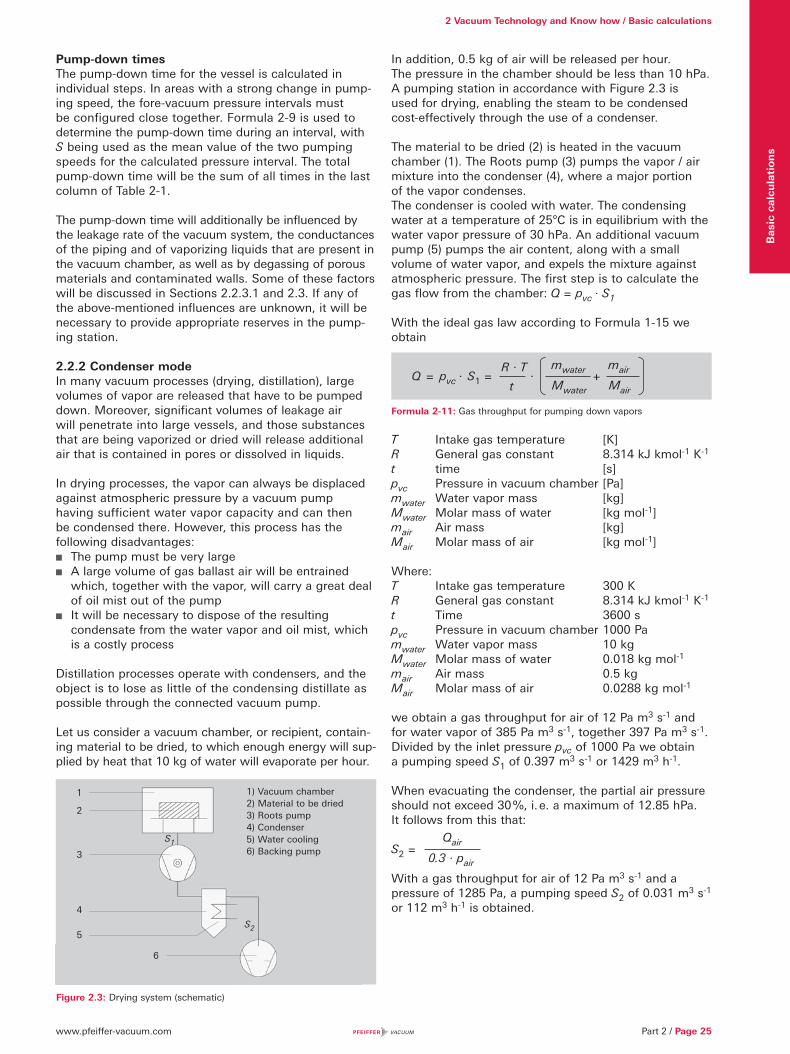
www.pfeiffer-vacuum.com Part 2 / Page 25
2 Vacuum Technology and Know how / Basic calculations
Bas
ic c
alcu
lati
on
s
Pump-down timesThe pump-down time for the vessel is calculated in individual steps. In areas with a strong change in pump-ing speed, the fore-vacuum pressure intervals must be configured close together. Formula 2-9 is used to determine the pump-down time during an interval, with S being used as the mean value of the two pumping speeds for the calculated pressure interval. The total pump-down time will be the sum of all times in the last column of Table 2-1.
The pump-down time will additionally be influenced by the leakage rate of the vacuum system, the conductances of the piping and of vaporizing liquids that are present in the vacuum chamber, as well as by de gassing of porous materials and contaminated walls. Some of these factors will be discussed in Sections 2.2.3.1 and 2.3. If any of the above-mentioned influences are unknown, it will be necessary to provide appropriate reserves in the pump-ing station.
2.2.2 Condenser modeIn many vacuum processes (drying, distillation), large volumes of vapor are released that have to be pumped down. Moreover, significant volumes of leakage air will penetrate into large vessels, and those substances that are being vaporized or dried will release additional air that is contained in pores or dissolved in liquids.
In drying processes, the vapor can always be displaced against atmospheric pressure by a vacuum pump having sufficient water vapor capacity and can then be condensed there. However, this process has the following disadvantages:
The pump must be very large A large volume of gas ballast air will be entrained
which, together with the vapor, will carry a great deal of oil mist out of the pump
It will be necessary to dispose of the resulting condensate from the water vapor and oil mist, which is a costly process
Distillation processes operate with condensers, and the object is to lose as little of the condensing distillate as possible through the connected vacuum pump.
Let us consider a vacuum chamber, or recipient, contain-ing material to be dried, to which enough energy will sup-plied by heat that 10 kg of water will evaporate per hour.
In addition, 0.5 kg of air will be released per hour. The pressure in the chamber should be less than 10 hPa. A pumping station in accordance with Figure 2.3 is used for drying, enabling the steam to be condensed cost-effectively through the use of a condenser.
The material to be dried (2) is heated in the vacuum chamber (1). The Roots pump (3) pumps the vapor / air mixture into the condenser (4), where a major portion of the vapor condenses.The condenser is cooled with water. The condensing water at a temperature of 25°C is in equilibrium with the water vapor pressure of 30 hPa. An additional vacuum pump (5) pumps the air content, along with a small volume of water vapor, and expels the mixture against atmospheric pressure. The first step is to calculate the gas flow from the chamber: Q = pvc · S1
With the ideal gas law according to Formula 1-15 we obtain
Formula 2-11: Gas throughput for pumping down vapors
T Intake gas temperature [K]R General gas constant 8.314 kJ kmol-1 K-1
t time [s]pvc Pressure in vacuum chamber [Pa]mwater Water vapor mass [kg]Mwater Molar mass of water [kg mol-1]mair Air mass [kg]Mair Molar mass of air [kg mol-1]
Where:T Intake gas temperature 300 KR General gas constant 8.314 kJ kmol-1 K-1
t Time 3600 spvc Pressure in vacuum chamber 1000 Pamwater Water vapor mass 10 kgMwater Molar mass of water 0.018 kg mol-1
mair Air mass 0.5 kgMair Molar mass of air 0.0288 kg mol-1
we obtain a gas throughput for air of 12 Pa m3 s-1 and for water vapor of 385 Pa m3 s-1, together 397 Pa m3 s-1. Divided by the inlet pressure pvc of 1000 Pa we obtain a pumping speed S1 of 0.397 m3 s-1 or 1429 m3 h-1.
When evacuating the condenser, the partial air pressure should not exceed 30 %, i. e. a maximum of 12.85 hPa. It follows from this that:
S2 =
With a gas throughput for air of 12 Pa m3 s-1 and a pressure of 1285 Pa, a pumping speed S2 of 0.031 m3 s-1 or 112 m3 h-1 is obtained.
1) Vacuum chamber2) Material to be dried3) Roots pump4) Condenser5) Water cooling6) Backing pump
1
2
3
4
6
5
S1
S2
Figure 2.3: Drying system (schematic)
Q = pvc · S1 = · +mwater mairR · T
Mwater Mairt
Qair
0.3 · pair
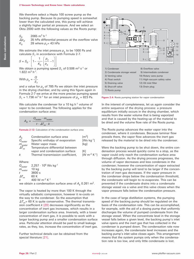
www.pfeiffer-vacuum.comPage 26 / Part 2
2 Vacuum Technology and Know how / Basic calculationsB
asic
cal
cula
tion
s
11
3
42
5
46
7
34
5
8
9
46
2
12
13
11
10
We therefore select a Hepta 100 screw pump as the backing pump. Because its pumping speed is somewhat lower than the calculated one, this pump will achieve a slightly higher partial air pressure. And we select an Okta 2000 with the following values as the Roots pump:
S0 2065 m³ h-1
� pd 35 hPa differential pressure at the overflow valveK0 28 where pv= 43 hPa
We estimate the inlet pressure pa to be 1000 Pa and calculate S1 in accordance with Formula 2-7.
S = S0 · 1 – – 1
We obtain a pumping speed S1 of 0.506 m3 s-1 or 1.822 m3 h-1.
With pa =
and a value for pa of 785 Pa we obtain the inlet pressure in the drying chamber, and by using this figure again in Formula 2-7 we arrive at the more precise pumping speed S1 = 1.736 m³ h-1 for an inlet pressure of pa = 823 Pa.
We calculate the condenser for a 10 kg h-1 volume of vapor to be condensed. The following applies for the condensation surface area:
Formula 2-12: Calculation of the condensation surface area
Ak Condensation surface area [m2]Qwater Specific enthalpy of evaporation [Ws kg-1]mwater Water vapor mass [kg]�Tm Temperature differential between vapor and condensation surface [K]k Thermal transmission coefficient, [W m-2 K-1]
Where:Qwater 2,257 · 106 Ws kg-1
mwater 10 kgt 3600 s�Tm 60 Kk 400 W m-2 K-1
we obtain a condensation surface area of Ak 0.261 m2.
The vapor is heated by more than 100 K through the virtually adiabatic compression, however it re-cools on the way to the condenser. So the assumption that � Tm= 60 K is quite conservative. The thermal transmis-sion coefficient k [20] decreases significantly as the concentration of inert gas increases, which results in a larger condensation surface area. Inversely, with a lower concentration of inert gas, it is possible to work with a larger backing pump and a smaller condensation surface area. Particular attention should be paid to small leakage rates, as they, too, increase the concentration of inert gas.
Further technical details can be obtained from the special literature [21].
Figure 2.4: Roots pumping station for vapor condensation
In the interest of completeness, let us again consider the entire sequence of the drying process: a pressure equilibrium initially occurs in the drying chamber, which results from the water volume that is being vaporized and that is caused by the heating-up of the material to be dried and the volume flow rate of the Roots pump.
The Roots pump advances the water vapor into the condenser, where it condenses. Because laminar flow prevails there, the vapor flow advances the inert gas released by the material to be dried into the condenser.
Were the backing pump to be shut down, the entire con-densation process would quickly come to a stop, as the vapor could only reach the condensation surface area through diffusion. As the drying process progresses, the volume of vapor decreases and less condenses in the condenser; however the concentration of vapor extracted by the backing pump will tend to be larger if the concen-tration of inert gas decreases. If the vapor pressure in the condenser drops below the condensation threshold, the condensate will begin to re-evaporate. This can be prevented if the condensate drains into a condensate storage vessel via a valve and this valve closes when the vapor pressure falls below the condensation pressure.
In the case of large distillation systems, the pumping speed of the backing pump should be regulated on the basis of the condensation rate. This can be accomplished, for example, with the aid of a dosing pump that uniformly discharges the volume of pumped condensate from the storage vessel. When the concentrate level in the storage vessel falls below a given level, the backing pump’s inlet valve opens and the inert gas that has collected in the condenser is pumped down. The condensation rate now increases again, the condensate level increases and the backing pump’s inlet valve closes again. This arrangement means that the system pumps only when the condensa-tion rate is too low, and only little condensate is lost.
1) Condenser
2) Condensate storage vessel
3) Venting valve
4) Float switch
5) Draining valve
6) Shut-off valve
7) Roots pump
8) Overflow valve
9) Intermediate condenser
10) Rotary vane pump
11) High-vacuum safety valve
12) Oil mist filter
13) Drain plug
1 pv
K0 pa
Q
S1
AK =Qwater · mwater
t · �Tm · k
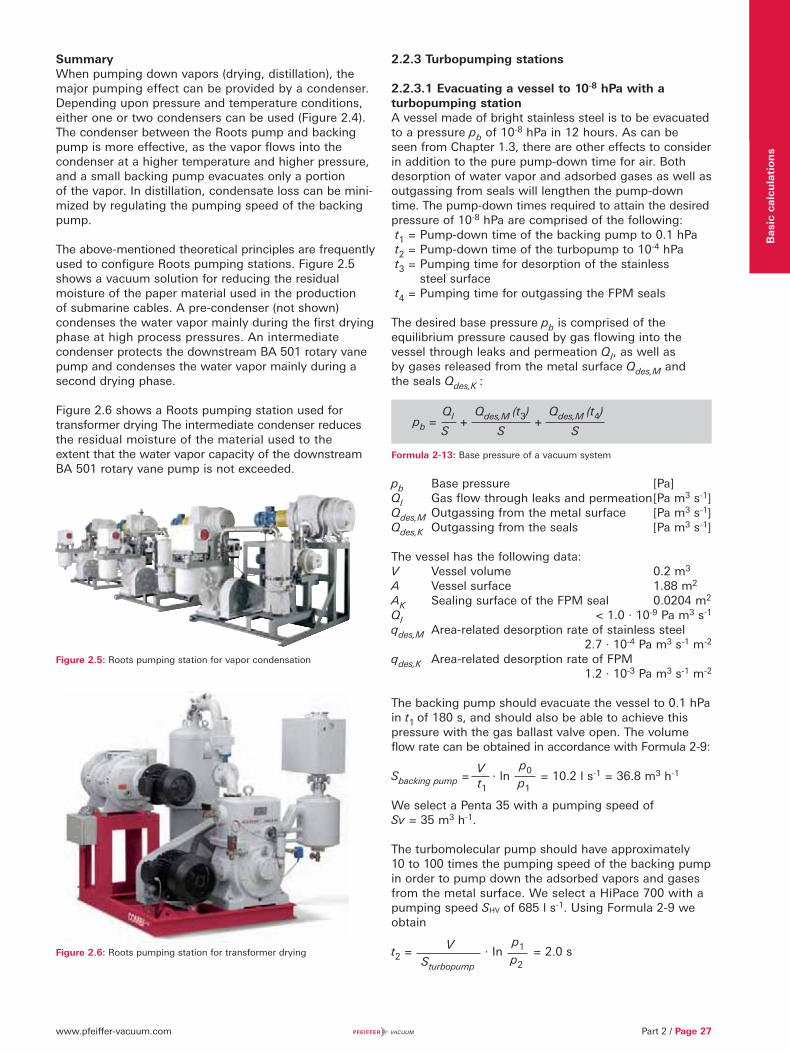
www.pfeiffer-vacuum.com Part 2 / Page 27
Intr
od
uct
ion
to
vacu
um
tec
hn
olo
gy
Bas
ic c
alcu
lati
on
s
SummaryWhen pumping down vapors (drying, distillation), the major pumping effect can be provided by a condenser. Depending upon pressure and temperature conditions, either one or two condensers can be used (Figure 2.4). The condenser between the Roots pump and backing pump is more effective, as the vapor flows into the condenser at a higher temperature and higher pressure, and a small backing pump evacuates only a portion of the vapor. In distillation, condensate loss can be mini-mized by regulating the pumping speed of the backing pump.
The above-mentioned theoretical principles are frequently used to configure Roots pumping stations. Figure 2.5 shows a vacuum solution for reducing the residual moisture of the paper material used in the production of submarine cables. A pre-condenser (not shown) condenses the water vapor mainly during the first drying phase at high process pressures. An intermediate condenser protects the downstream BA 501 rotary vane pump and condenses the water vapor mainly during a second drying phase.
Figure 2.6 shows a Roots pumping station used for transformer drying The intermediate condenser reduces the residual moisture of the material used to the extent that the water vapor capacity of the downstream BA 501 rotary vane pump is not exceeded.
Figure 2.5: Roots pumping station for vapor condensation
Figure 2.6: Roots pumping station for transformer drying
2.2.3 Turbopumping stations
2.2.3.1 Evacuating a vessel to 10-8 hPa with a turbopumping stationA vessel made of bright stainless steel is to be evacuated to a pressure pb of 10-8 hPa in 12 hours. As can be seen from Chapter 1.3, there are other effects to consider in addition to the pure pump-down time for air. Both desorption of water vapor and adsorbed gases as well as outgassing from seals will lengthen the pump-down time. The pump-down times required to attain the desired pressure of 10-8 hPa are comprised of the following: t1 = Pump-down time of the backing pump to 0.1 hPa t2 = Pump-down time of the turbopump to 10-4 hPa t3 = Pumping time for desorption of the stainless
steel surface t4 = Pumping time for outgassing the FPM seals
The desired base pressure pb is comprised of the equilibrium pressure caused by gas flowing into the vessel through leaks and permeation QI, as well as by gases released from the metal surface Qdes,M and the seals Qdes,K :
Formula 2-13: Base pressure of a vacuum system
pb Base pressure [Pa]Ql Gas flow through leaks and permeation [Pa m3 s-1]Qdes,M Outgassing from the metal surface [Pa m3 s-1]Qdes,K Outgassing from the seals [Pa m3 s-1]
The vessel has the following data:V Vessel volume 0.2 m3
A Vessel surface 1.88 m2
AK Sealing surface of the FPM seal 0.0204 m2
Ql < 1.0 · 10-9 Pa m3 s-1
qdes,M Area-related desorption rate of stainless steel 2.7 · 10-4 Pa m3 s-1 m-2
qdes,K Area-related desorption rate of FPM1.2 · 10-3 Pa m3 s-1 m-2
The backing pump should evacuate the vessel to 0.1 hPa in t1 of 180 s, and should also be able to achieve this pressure with the gas ballast valve open. The volume flow rate can be obtained in accordance with Formula 2-9:
Sbacking pump = · ln = 10.2 l s-1 = 36.8 m3 h-1
We select a Penta 35 with a pumping speed of Sv = 35 m3 h-1.
The turbomolecular pump should have approximately 10 to 100 times the pumping speed of the backing pump in order to pump down the adsorbed vapors and gases from the metal surface. We select a HiPace 700 with a pumping speed SHV of 685 l s-1. Using Formula 2-9 we obtain
t2 = · In = 2.0 s
pb = + + Ql
S
Qdes,M (t3)
S
Qdes,M (t4)
S
Vt1
p0
p1
VSturbopump
p1
p2
www.pfeiffer-vacuum.comPage 28 / Part 2
2 Vacuum Technology and Know how / Basic calculationsB
asic
cal
cula
tion
s
Desorption from the surface of the vesselGas molecules (primarily water) adsorb on the interior surfaces of the pressure chamber and gradually vaporize again under vacuum. The desorption rates of metal surfaces decline at a rate of t -1. Time constant t0 is approximately 1 h.
Using Formula 1-32 from Chapter 1
we calculate the time taken to attain the base pressure
pb3 = 1.0 · 10-6 Pa
t3 = = 2.67 · 106 s = 741 h.
The resulting time of 741 hours is too long. The process must be shortened by baking out the vessel. The bakeout temperature is selected so as to prevent harming the most temperature-sensitive of the materials used. In our example, the temperature is restricted by the use of FPM seals which can easily withstand a temperature of 370 K. The desorption speed will be increased theoretically by more than a factor of 1,000 as a result [22]. And the bake-out time will in effect be shortened to several hours.
High desorption rates can also be lowered by annealing the vessel under vacuum or by means of certain surface treatments (polishing, pickling).
Since many pre-treatment influences play a role, precise prediction of the pressure curve over time is not possible. However in the case of bake out temperatures of around 150°C, it will suffice to turn off the heater after attaining a pressure that is higher by a factor of 100 than the desired base pressure. The desired pressure pb3 will then be attained after the vacuum chamber has cooled down.
Seal desorptionThe outgassing rates of plastic are important if operation is at temperatures of below 10-6 hPa. Although the surface areas of the seals are relatively small, desorption decreases only according to the factor
given in Formula 1-33 in Chapter 1.
The reason for this is that the escaping gases are not only bound on the surface, but must also diffuse out of the interior of the seal. With extended pumping times, desorption from plastics can therefore dominate desorption from the metal surfaces. The outgassing rate of plastic surfaces is calculated according to Formula 1-33 in Chapter 1.
We use Qdes,K = S · pdes,K and obtain the following for
pb4 = 10-8 hPa: t4 = 459 · 106 s = 1277 h.
In this connection t0 = 3600 s and the associated value qdes,K is read from the chart [23] for FPM. It can be seen that the contribution to pump-down time made by desorption of the cold-state seal is of a similar order of magnitude as that of the metal surface.
Since the diffusion of the gases released in the interior of the seal will determine the behavior of the desorption gas flow over time, the dependence of diffusion coeffi-cient D upon temperature will have a crucial influence on pumping time:
Formula 2-14: Diffusion coefficient (T)
As temperature rises, the diffusion coefficient increases as well; however it will not rise as sharply as the desorp-tion rate of the metal surface. As a result, we see that elastomer seals can have a pronouncedly limiting effect on base pressure due to their desorption rates, which is why they are not suitable for generating ultra-high vacuum.
Leakage rate and permeation rateThe gas flow that enters the vacuum system through leaks is constant and at a given pumping speed results in a pressure of:
pleak =
A system is considered to be sufficiently tight if this pressure is less than 10% of the working pressure. Leakage rates of 10-9 Pa m3 s-1 are usually easy to attain and are also required for this system. This results in a pressure component of the leakage rate of pleak = 1.46 · 10-11 hPa. This value is not disturbing and can be left out of consideration.
Permeation rates through metal walls do not influence the ultimate pressure that is required in this example; however diffusion through elastomer seals can also have a limiting effect on base pressure in the selected example.
SummaryPressures of up to 10-7 hPa can be attained in approxi-mately one day in clean vessels without the need for any additional measures.
If pressures of up to 10-4 hPa are to be attained, the pump-down times of the backing pump and the turbo-pump must be added together. In the above-mentioned case, this is approximately 200 s. At pressures of less than 10-6 hPa, the turbomolecular pump is required to have a high pumping speed, particularly in order to pump down the water desorbed from the metal walls.
This will only be possible by additionally baking out the vacuum vessel (90 to 400°C) if the required base pres-sure pb of 10-8 hPa is to be attained within a few hours. The heater is turned off after 100 times the value of the
Qdes = qdes · A ·t0t3
qdes,M · A · t0S · pb3
t0 t4
Qdes,K = qdes,K · Ad ·t0
t4
D = D0 · exp –Edif
R · T
Qleak
S
www.pfeiffer-vacuum.com
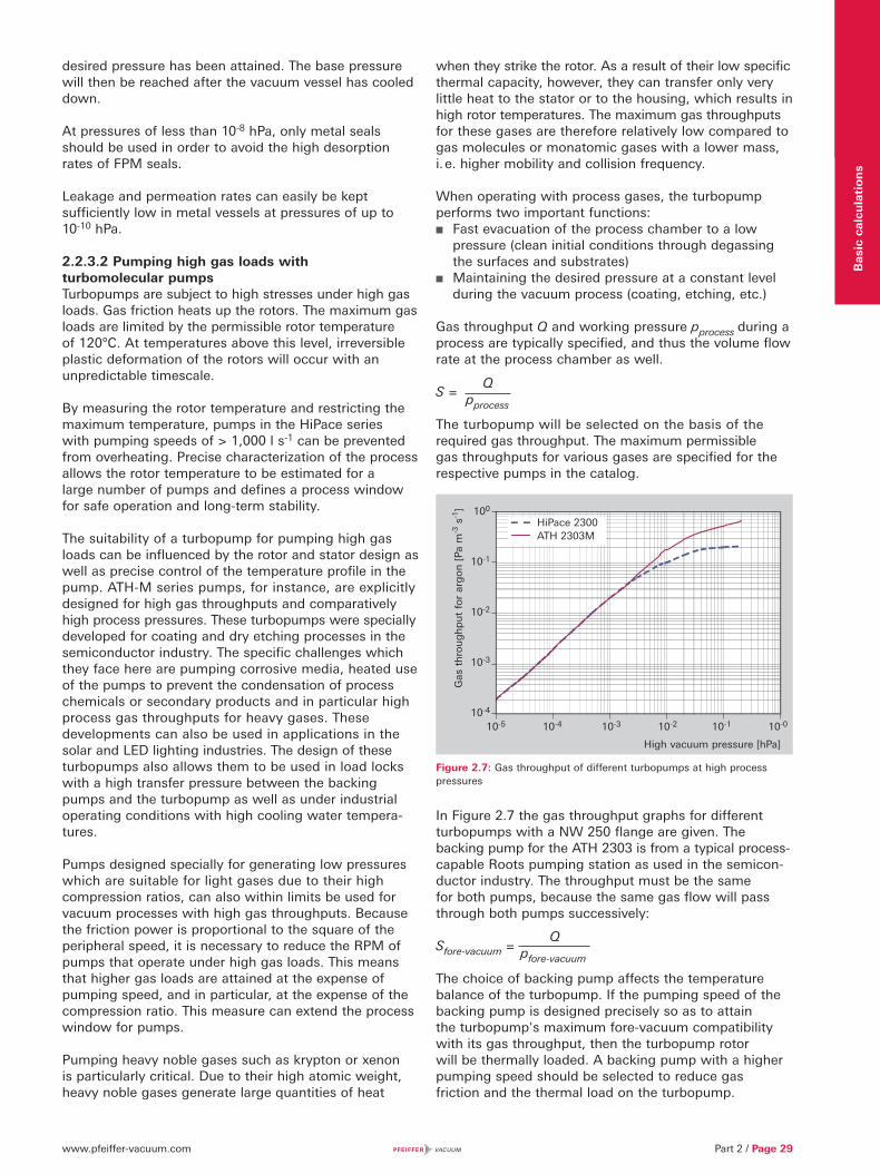
www.pfeiffer-vacuum.com Part 2 / Page 29
Intr
od
uct
ion
to
vacu
um
tec
hn
olo
gy
Bas
ic c
alcu
lati
on
s
when they strike the rotor. As a result of their low specific thermal capacity, however, they can transfer only very little heat to the stator or to the housing, which results in high rotor temperatures. The maximum gas throughputs for these gases are therefore relatively low compared to gas molecules or monatomic gases with a lower mass, i. e. higher mobility and collision frequency.
When operating with process gases, the turbopump performs two important functions:
Fast evacuation of the process chamber to a low pressure (clean initial conditions through degassing the surfaces and substrates)
Maintaining the desired pressure at a constant level during the vacuum process (coating, etching, etc.)
Gas throughput Q and working pressure pprocess during a process are typically specified, and thus the volume flow rate at the process chamber as well.
S =
The turbopump will be selected on the basis of the required gas throughput. The maximum permissible gas throughputs for various gases are specified for the respective pumps in the catalog.
Figure 2.7: Gas throughput of different turbopumps at high process pressures
In Figure 2.7 the gas throughput graphs for different turbopumps with a NW 250 flange are given. The backing pump for the ATH 2303 is from a typical process-capable Roots pumping station as used in the semicon-ductor industry. The throughput must be the same for both pumps, because the same gas flow will pass through both pumps successively:
Sfore-vacuum =
The choice of backing pump affects the temperature balance of the turbopump. If the pumping speed of the backing pump is designed precisely so as to attain the turbopump's maximum fore-vacuum compatibility with its gas throughput, then the turbopump rotor will be thermally loaded. A backing pump with a higher pumping speed should be selected to reduce gas friction and the thermal load on the turbopump.
desired pressure has been attained. The base pressure will then be reached after the vacuum vessel has cooled down.
At pressures of less than 10-8 hPa, only metal seals should be used in order to avoid the high desorption rates of FPM seals.
Leakage and permeation rates can easily be kept sufficiently low in metal vessels at pressures of up to 10-10 hPa.
2.2.3.2 Pumping high gas loads with turbomolecular pumpsTurbopumps are subject to high stresses under high gas loads. Gas friction heats up the rotors. The maximum gas loads are limited by the permissible rotor temperature of 120°C. At temperatures above this level, irreversible plastic deformation of the rotors will occur with an unpredictable timescale.
By measuring the rotor temperature and restricting the maximum temperature, pumps in the HiPace series with pumping speeds of > 1,000 l s-1 can be prevented from overheating. Precise characterization of the process allows the rotor temperature to be estimated for a large number of pumps and defines a process window for safe operation and long-term stability.
The suitability of a turbopump for pumping high gas loads can be influenced by the rotor and stator design as well as precise control of the temperature profile in the pump. ATH-M series pumps, for instance, are explicitly designed for high gas throughputs and comparatively high process pressures. These turbopumps were specially developed for coating and dry etching processes in the semiconductor industry. The specific challenges which they face here are pumping corrosive media, heated use of the pumps to prevent the condensation of process chemicals or secondary products and in particular high process gas throughputs for heavy gases. These developments can also be used in applications in the solar and LED lighting industries. The design of these turbopumps also allows them to be used in load locks with a high transfer pressure between the backing pumps and the turbopump as well as under industrial operating conditions with high cooling water tempera-tures.
Pumps designed specially for generating low pressures which are suitable for light gases due to their high compression ratios, can also within limits be used for vacuum processes with high gas throughputs. Because the friction power is proportional to the square of the peripheral speed, it is necessary to reduce the RPM of pumps that operate under high gas loads. This means that higher gas loads are attained at the expense of pumping speed, and in particular, at the expense of the compression ratio. This measure can extend the process window for pumps.
Pumping heavy noble gases such as krypton or xenon is particularly critical. Due to their high atomic weight, heavy noble gases generate large quantities of heat
Qpprocess
Qpfore-vacuum
100
10-1
10-2
10-3
10-4
Gas
th
rou
gh
pu
t fo
r ar
go
n [
Pa
m-3
s-1
]
HiPace 2300ATH 2303M
High vacuum pressure [hPa]
10-5 10-4 10-3 10-2 10-1 10-0
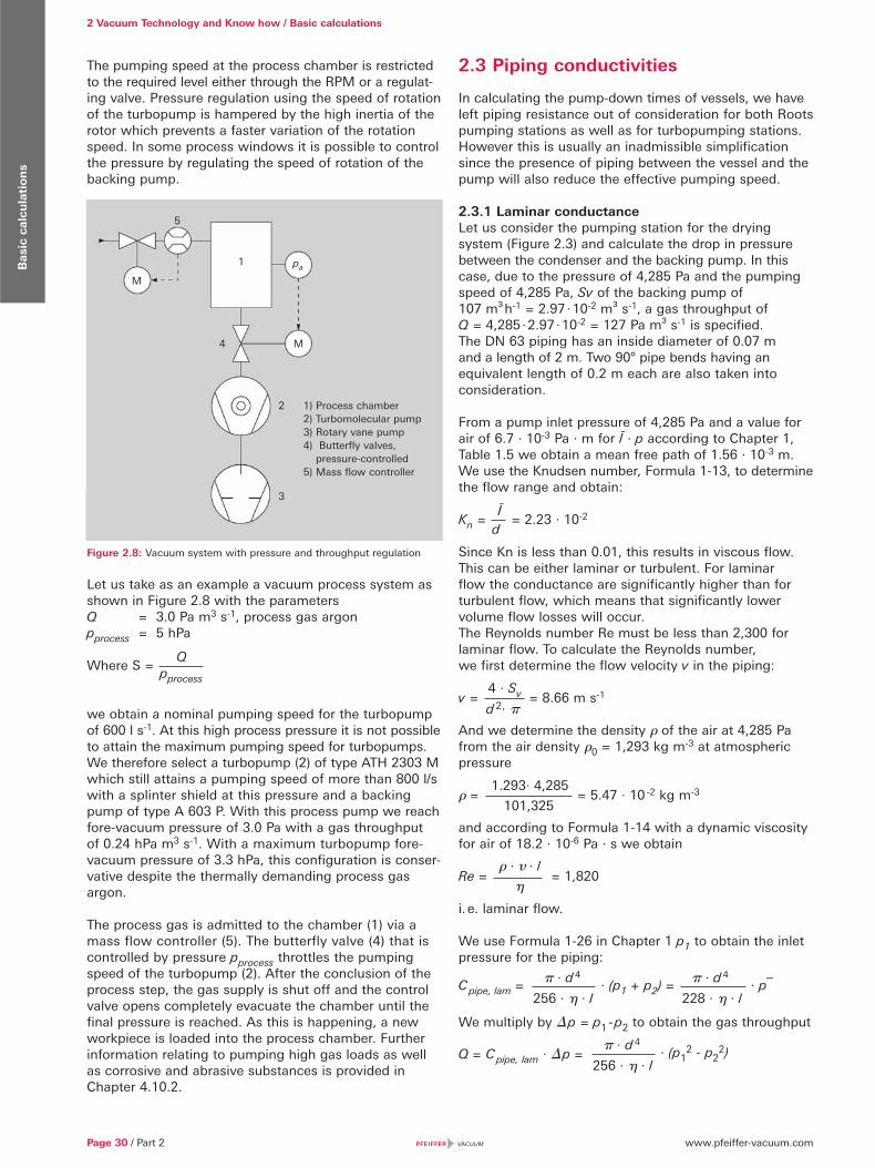
www.pfeiffer-vacuum.comPage 30 / Part 2
2 Vacuum Technology and Know how / Basic calculationsB
asic
cal
cula
tion
s
The pumping speed at the process chamber is restricted to the required level either through the RPM or a regulat-ing valve. Pressure regulation using the speed of rotation of the turbopump is hampered by the high inertia of the rotor which prevents a faster variation of the rotation speed. In some process windows it is possible to control the pressure by regulating the speed of rotation of the backing pump.
Figure 2.8: Vacuum system with pressure and throughput regulation
Let us take as an example a vacuum process system as shown in Figure 2.8 with the parameters Q = 3.0 Pa m3 s-1, proc ess gas argonpprocess = 5 hPa
Where S =
we obtain a nominal pumping speed for the turbopump of 600 l s-1. At this high process pressure it is not possible to attain the maximum pumping speed for turbopumps. We therefore select a turbopump (2) of type ATH 2303 M which still attains a pumping speed of more than 800 l/s with a splinter shield at this pressure and a backing pump of type A 603 P. With this process pump we reach fore-vacuum pressure of 3.0 Pa with a gas throughput of 0.24 hPa m3 s-1. With a maximum turbopump fore-vacuum pressure of 3.3 hPa, this configuration is conser-vative despite the thermally demanding process gas argon.
The process gas is admitted to the chamber (1) via a mass flow controller (5). The butterfly valve (4) that is controlled by pressure pprocess throttles the pumping speed of the turbopump (2). After the conclusion of the process step, the gas supply is shut off and the control valve opens completely evacuate the chamber until the final pressure is reached. As this is happening, a new workpiece is loaded into the process chamber. Further information relating to pumping high gas loads as well as corrosive and abrasive substances is provided in Chapter 4.10.2.
2.3 Piping conductivities
In calculating the pump-down times of vessels, we have left piping resistance out of consideration for both Roots pumping stations as well as for turbopumping stations. However this is usually an inadmissible simplification since the presence of piping between the vessel and the pump will also reduce the effective pumping speed.
2.3.1 Laminar conductanceLet us consider the pumping station for the drying system (Figure 2.3) and calculate the drop in pressure between the condenser and the backing pump. In this case, due to the pressure of 4,285 Pa and the pumping speed of 4,285 Pa, Sv of the backing pump of 107 m³ h-1 = 2.97 · 10-2 m³ s-1, a gas throughput of Q = 4,285 · 2.97 · 10-2 = 127 Pa m³ s-1 is specified. The DN 63 piping has an inside diameter of 0.07 m and a length of 2 m. Two 90° pipe bends having an equivalent length of 0.2 m each are also taken into consideration.
From a pump inlet pressure of 4,285 Pa and a value for air of 6.7 · 10-3 Pa · m for Ī · p according to Chapter 1, Table 1.5 we obtain a mean free path of 1.56 · 10-3 m. We use the Knudsen number, Formula 1-13, to determine the flow range and obtain:
Kn = = 2.23 · 10-2
Since Kn is less than 0.01, this results in viscous flow. This can be either laminar or turbulent. For laminar flow the conductance are significantly higher than for turbulent flow, which means that significantly lower volume flow losses will occur. The Reynolds number Re must be less than 2,300 for laminar flow. To calculate the Reynolds number, we first determine the flow velocity v in the piping:
v = = 8.66 m s-1
And we determine the density � of the air at 4,285 Pa from the air density �0 = 1,293 kg m-3 at atmospheric pressure
� = = 5.47 · 10 -2 kg m-3
and according to Formula 1-14 with a dynamic viscosity for air of 18.2 · 10-6 Pa · s we obtain
Re = = 1,820
i. e. laminar flow.
We use Formula 1-26 in Chapter 1 p1 to obtain the inlet pressure for the piping:
We multiply by � p = p1 - p2 to obtain the gas throughput
1
1) Process chamber2) Turbomolecular pump3) Rotary vane pump4) Butterfly valves,
pressure-controlled5) Mass flow controller
2
3
4 M
pa
5
M
Qpprocess
Ī d
C pipe, lam = · (p1 + p2) = · p–� · d 4
256 · � · l
� · d 4
228 · � · l
Q = C pipe, lam · � p = · (p12 - p2
2)� · d 4
256 · � · l
� · � · l
�
4 · Sv
d 2· �
1.293· 4,285
101,325
www.pfeiffer-vacuum.com Part 2 / Page 31
2 Vacuum Technology and Know how / Basic calculations
Bas
ic c
alcu
lati
on
s
Since p2 = 4,285 Pa and Q = 127 Pa · m3 s-1 it is possible to directly determine p1 from these values:
p1 = qdiff · Ad · p2 2 + = 4,287.2 Pa
We have a pressure loss of merely 2.2 Pa, a very low value.
The conductivity of the piping is obtained from Chapter 1, Formula 1-18:
C = = 58 m3 s-1 or 58,000 l s-1
The effective volume flow rate
Seff = = 2.9707 m3 s-1
is only slightly lower than the volume flow rate without the piping: Sv of 2.9222 m3 s-1.
2.3.2 Molecular conductanceNow let us also consider the conductance of the same piping in the molecular flow range. The piping has a diameter of 0.07 m and a length of 2 m. The elongated length of 0.235 each of the two 90° pipe bends, i. e. a total length of l = 2.47 m. In accordance with Chapter 1, Formula 1-30, the piping resistance is:
LRm = = 1.71 · 10-2 m3 s-1
where c– = 471 m s-1 for air at T = 293 K. The orifice conductivity of the pipe inlet has already been taken into account.
The effective volume flow rate is obtained with the following formula:
In the molecular flow range, the pumping speed of the backing pump would be reduced to nearly one third. In this range, it is absolutely necessary to pay strict attention to short runs and large piping cross sections between the pump and the vacuum chamber. This applies in particular for turbopumps that should ideally be flanged directly to the vacuum chamber.
Q · 256 · � · l� · d 4
Q
� p
Sv · Cpipe, lam
Sv + Cpipe, lam
c– · � · d 3
12 · l
Sv · LRm
Sv + LRmSeff = = 1.09 · 10-2 m3 s-1 where SV = 2.97 · 10-2 m3 s-1
www.pfeiffer-vacuum.comPage 32 / Part 2
Mec
han
ical
com
po-
nen
ts in
vac
uu
m
3 Mechanical components in vacuum
3.1 General
A vacuum system includes a variety of different compo-nents, such as chambers, pumps, measurement instru-ments, components, valves, feedthroughs, manipulators, etc., that must be joined together to form a unit. A dis-tinction is made between detachable connections, which are equipped with seals, and non-detachable connections. The following sections describe the materials used in vacuum technology, the different types of connections and the mechanical components. It shows what to look out for during the design and the selection.
3.2 MaterialsIn vacuum technology, the requirements placed on any material are very diverse. Depending on the application, ambient conditions and the vacuum to be achieved, it must be tested which requirements the materials must meet.
The following lists important requirements that must be considered:
Sufficient mechanical strength throughout the entire operational temperature range: in addition to the structural integrity, it must be ensured that the deformation of the functional surfaces does not impact the functionality. Example: The atmospheric air pressure on evacuated chamber components is approximately 10 N/cm2. With an area of 1 m2, this results in a force of 100,000 N.
High gas tightness: Each material is basically gas permeable. The overall process of gas permeability is called permeation. It depends on the material, the type of gas and the ambient conditions – especially the temperature. With the use of elastomer seals, their permeation must be considered. Example: For an FKM (fluoroelas-tomer) seal of DN 500 ISO-K, the permeation rate for atmospheric air with 60 % humidity is about 4 · 10-7 Pa · m3/s. Therefore typical vacuum systems with FKM seals rarely achieve a working pressure of more than 1 · 10-8 hPa.
Low intrinsic vapor pressure, high melting and boiling point: Intrinsic vapor pressure that is too high limits the final vacuum pressure. In addition to the vacuum compati-bility of oils and grease, the intrinsic vapor pressure of metals or their partial pressure in alloys must be con-
sidered in alloys. Example: For brass, the partial pressure of the zinc is limited to a maximum permissi-ble temperature in a high vacuum at about 100°C.
Clean surfaces, low content of foreign gases, easy degassing: Clean surfaces are a prerequisite. However, any surface that was exposed to the ambient air, is coated with an adsorbed layer. Chemically or physically adsorbed molecules on the surface or in the volume of the material represent a source of gas once they desorb (when they detach from surface). To achieve a low final pressure, materials with low desorption rates must be used. Example: A monolayer of adsorbed gas roughly equals a gas quantity of 4 · 10-2 Pa · m3/m2. Considering a pipe, closed at both ends, with a diameter of 50 cm and a length of 100 cm (surface area of about 2 m2, volume approx. 200 l), the release of the monolayer results in a pressure rise of about 0.4 Pa or 4 · 10-3 hPa. This does not take into account the fact that the surface is always larger than the geometric area.
Good thermal shock resistance, adjusted expansion behavior: Example: The different thermal expansion limits the maximum permissible temperature for the combination of aluminum seal and stainless steel flanges to about 150°C. Often after too high temperatures, a deterioration in the sealing effect occurs during cooling.
Corrosion resistance, chemical resistance: Example: A lot of coating processes require chemically active process gases. It is therefore necessary to consider whether the fluids used affect components or seals. In particular, thin-walled components such as metal bellows are vulnerable to corrosion. If necessary, their service life should be determined in tests.
Special applications may also place further demands on the materials.As a general rule: the lower the desired working pres-sure, the greater the demands placed on the material and the smaller the selection of possible materials. Therefore, especially in UHV (ultra-high vacuum) technology, the choice of materials is of great importance.
3.2.1 Metallic materials Many metals and metal alloys have high strength, are easy to process and clean, temperature resistant and less sensitive to mechanical influences than glass. The consideration of economic aspects, such as the material
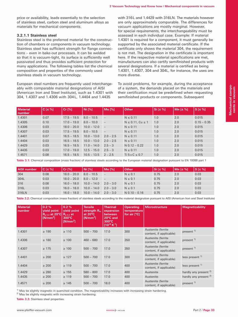
www.pfeiffer-vacuum.com Part 2 / Page 33
2 Vacuum Technology and Know how / Mechanical components in vacuum
Mec
han
ical
com
po-
nen
ts in
vac
uu
m
price or availability, leads essentially to the selection of stainless steel, carbon steel and aluminum alloys as materials for mechanical components.
3.2.1.1 Stainless steelStainless steel is the preferred material for the construc-tion of chambers or components in vacuum technology. Stainless steel has sufficient strength for flange connec-tions – even in bake-out processes. It can be welded so that it is vacuum-tight, its surface is sufficiently well passivated and thus provides sufficient protection for many applications. The following tables list the chemical composition and properties of the commonly used stainless steels in vacuum technology.
European steel numbers are frequently used interchange-ably with comparable material designations of AISI (American Iron and Steel Institute), such as 1.4301 with 304, 1.4307 and 1.4306 with 304 L, 1.4404 and 1.4435
with 316 L and 1.4429 with 316LN. The materials however are only approximately comparable. The differences for vacuum applications are mostly marginal. However, for special requirements, the interchangeability must be assessed in each individual case. Example: If material 1.4301 is required for a component, it must generally be supported by the associated material certificate. If the certificate only shows the material 304, the requirement is not met. The designation in the certificate is important here. If the respective material specifications are met, manufacturers can also certify semifinished products with several designations. If a material is certified as being 1.4301, 1.4307, 304 and 304L, for instance, the uses are more diverse.
To avoid problems, for example, during the acceptance of a system, the demands placed on the materials and their certification must be predefined when requesting semifinished products or components. Subsequent
Material number
C [≤ %] Cr [%] Ni [%] Mo [%] Other Si [≤ %] Mn [≤ %] S [≤ %]
1.4301 0.07 17.5 – 19.5 8.0 – 10.5 – N ≤ 0.11 1.0 2.0 0.015
1.4305 0.10 17.0 – 19.0 8.0 – 10.0 – N ≤ 0.11, Cu ≤ 1 1.0 2.0 0.15 – 0.35
1.4306 0.03 18.0 – 20.0 10.0 – 12.0 – N ≤ 0.11 1.0 2.0 0.015
1.4307 0.03 17.5 – 19.5 8.0 – 10.5 – N ≤ 0.11 1.0 2.0 0.015
1.4401 0.07 16.5 – 18.5 10.0 – 13.0 2.0 – 2.5 N ≤ 0.11 1.0 2.0 0.015
1.4404 0.03 16.5 – 18.5 10.0 – 13.0 2.0 – 2.5 N ≤ 0.11 1.0 2.0 0.015
1.4429 0.03 16.5 – 18.5 11.0 – 14.0 2.5 – 3 N 0.12 – 0.22 1.0 2.0 0.015
1.4435 0.03 17.0 – 19.0 12.5 – 15.0 2.5 – 3 N ≤ 0.11 1.0 2.0 0.015
1.4571 0.08 16.5 – 18.5 10.5 – 13.5 2 – 2.5 Ti 5 × C ≤ 0.7 1.0 2.0 0.015
Table 3.1: Chemical composition (mass fraction) of stainless steels according to the European material designation pursuant to EN 10088 part 1
AISI number C [≤ %] Cr [%] Ni [%] Mo [%] Other Si [≤ %] Mn [≤ %] S [≤ %]
304 0.08 18.0 – 20.0 8.0 – 10.5 – N ≤ 0.1 0.75 2.0 0.03
304L 0.03 18.0 – 20.0 8.0 – 12.0 – N ≤ 0.1 0.75 2.0 0.03
316 0.08 16.0 – 18.0 10.0 – 14.0 2.0 – 3.0 N ≤ 0.1 0.75 2.0 0.03
316L 0.03 16.0 – 18.0 10.0 – 14.0 2.0 – 3.0 N ≤ 0.1 0.75 2.0 0.03
316LN 0.03 16.0 – 18.0 10.0 – 14.0 2.0 – 3.0 N 0.10 – 0.16 0.75 2.0 0.03
Table 3.2: Chemical composition (mass fraction) of stainless steels according to the material designation pursuant to AISI (American Iron and Steel Institute)
Material number
0.2 % yield point Rp 0.2 at 20°C [N/mm2]
0.2 % yield point Rp 0.2 at 300°C [N/mm2]
Tensile strength Rm at 20°C [N/mm2]
Thermal expansion between 20°C and 300°C [10-6 K-1]
Operating temperature for air [°C]
Microstructure Magnetizability
1.4301 ≥ 190 ≥ 110 500 – 700 17.0 300Austenite (ferrite content, if applicable)
present 1)
1.4306 ≥ 180 ≥ 100 460 – 680 17.0 350Austenite (ferrite content, if applicable)
present 1)
1.4307 ≥ 175 ≥ 100 500 – 700 17.0 350Austenite (ferrite content, if applicable)
present 1)
1.4401 ≥ 200 ≥ 127 500 – 700 17.0 300Austenite (ferrite content, if applicable)
less present 1)
1.4404 ≥ 200 ≥ 119 500 – 700 17.0 400Austenite (ferrite content, if applicable)
less present 1)
1.4429 ≥ 280 ≥ 155 580 – 800 17.0 400 Austenite hardly any present 2)
1.4435 ≥ 200 ≥ 119 500 – 700 17.0 400 Austenite hardly any present 2)
1.4571 ≥ 200 ≥ 145 500 – 700 18.0 400Austenite (ferrite content, if applicable)
present 1)
1) May be slightly magnetic in quenched condition. The magnetizability increases with increasing strain hardening.2) May be slightly magnetic with increasing strain hardening.
Table 3.3: Stainless steel properties

www.pfeiffer-vacuum.comPage 34 / Part 2
2 Vacuum Technology and Know how / Mechanical components in vacuumM
ech
anic
al C
om
po-
nen
ts in
Vac
uu
m
certification is often not possible, especially for special requirements: for example, due to special mechanical properties, a restriction in the chemical composition or the certification according to AD 2000 W2 (Working Group for Pressure Vessels 2000 date sheet W2, “Materials for pressure vessels”) or the ASME (American Society of Mechanical Engineers).
Stainless steel 1.4301: the most frequently used chromium-nickel steel. Excellent cold forming, welding and polishing properties. Sufficient corrosion resistance for many applications. Suitable for vacuum applications. Used, for example, for flanges, pipe components and chambers.
Stainless steel 1.4305: Variant of 1.4301 with sulfur con-tent to improve machinability (machining steel). Lower corrosion resistance than 1.4301. Non-weldable. Suffi-ciently well-suited for vacuum applications. Use in part for turned and milling parts, such as centering rings.
Stainless steel 1.4307, 1.4306: low carbon variant of 1.4301. Due to the low carbon content it is weldable, without being susceptible to intergranular corrosion. Slightly lower strength than 1.4301. Highly suitable for vacuum applications. For uses requiring a very low carbon content, e. g. for CF flanges. 1.4307 is increasingly replacing 1.4306, as the benefits associated with the higher chromium and nickel content are often not suffi-cient to justify the higher purchase costs.
Stainless steel 1.4401: excellent cold forming properties. Good weldability and polishability. Due to the molybde-num additive it is more resistant than 1.4301 to non- oxidizing acids and chloride ion-containing media. Well suited for vacuum applications. Used for example for valve housings, in areas which require greater protection against corrosion, or for domestic drinking water systems.
Stainless steel 1.4404: low carbon variant of 1.4401. Due to the low carbon content it is weldable, without being susceptible to intergranular corrosion. Highly suitable for vacuum applications. It is used when a very low carbon content or greater corrosion resistance is required, for example, for pipes and flange components in the semiconductor industry.
Stainless steel 1.4435: the higher nickel content com-pared to 1.4404 stabilizes the austenitic structure, reduces the formation of delta ferrite and is therefore barely magnetic even in the welded seam area. Due to the increased molybdenum additive it is more resistant than 1.4404 to non-oxidizing acids and chloride ion-containing media. Highly suitable for vacuum applications. It is often used in the pharmaceutical industry, also according to the Basel Standard 2 (BN2), which sets tougher ana-lytical limits and defines the permissible ferrite content.
Stainless steel 1.4429: similar characteristics as 1.4435, however, greater strength due to the high nitrogen content. This also stabilizes the austenitic structure, thereby minimizing the formation of delta ferrite and thus the magnetization. Highly suitable for vacuum applications. It is used for CF flanges, especially when vacuum annealing for cleaning or demagnetization occurs at high temperatures. The availability for tubes and sheet metal from 1.4429 is low. Therefore, flanges from 1.4429 for chambers or components are often combined with semifinished products made of 1.4404 or 1.4307.
Stainless steel 1.4429 ESR: Same properties as for 1.4429, but improved microstructure and higher purity due to the ESR (electroslag remelting process) treat-ment. Exceptionally well suited for vacuum applications. It is used as a premium quality for CF flanges that exhib-it great strength and minimal magnetizability, combined with the high chemical purity and homogeneity of the structure.
Stainless steel 1.4571: classic “V4A” steel with high availability. Stabilized with titanium and therefore weldable without being susceptible to intergranular corrosion. Similar properties to 1.4401, however, due to the titanium carbides in the structure, it is only moderately polishable and not suited for electro-polish-ing. Well suited for vacuum applications. Used for example for piping and apparatus construction, where greater corrosion resistance is required.
ESR (electroslag remelting process): through the ESR process, dense and low-segregation stainless steels, with high chemical and structural purity are produced
Figure 3.1: Temperature dependence of the elasticity modulus of austenitic stainless steel
Figure 3.2: Temperature dependence of the 0.2% yield point of austenitic stainless steel
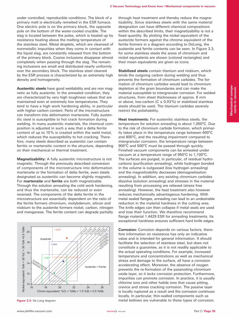
www.pfeiffer-vacuum.com Part 2 / Page 35
2 Vacuum Technology and Know how / Mechanical components in vacuum
Mec
han
ical
com
po-
nen
ts in
vac
uu
m
under controlled, reproducible conditions. The block of a primary melt is electrically remelted in the ESR furnace. One electric pole is on the primary block, the opposite pole on the bottom of the water-cooled crucible. The slag is located between the poles, which is heated up by resistance heating above the melting temperature of the stainless steel. Metal droplets, which are cleansed of nonmetallic impurities when they come in contact with the liquid slag, are constantly released from the bottom of the primary block. Coarse inclusions disappear almost completely when passing through the slag. The remain-ing inclusions are small and distributed nearly uniformly over the secondary block. The stainless steel cleaned by the ESR process is characterized by an extremely high density and homogeneity.
Austenitic steels have good weldability and are non mag-netic as fully austenite. In the annealed condition, they are characterized by very high toughness values that are maintained even at extremely low temperatures. They tend to have a high work hardening ability, in particular with higher carbon content. Parts of the microstructure can transform into deformation martensite. Fully austen-itic steel is susceptible to hot crack formation during welding. In many austenitic materials, the chemical com-position is adjusted in such a way that a delta ferrite content of up to 10 % is created within the weld metal, which reduces the susceptibility to hot cracking. There-fore, many steels described as austenitic can contain ferritic or martensitic content in the structure, depending on their mechanical or thermal treatment.
Magnetizability: A fully austenitic microstructure is not magnetic. Through the previously described conversion of components of the microstructure into deformation martensite or the formation of delta ferrite, even steels designated as austenitic can become slightly magnetic. For martensite and ferrite are both magnetizable. Through the solution annealing the cold work hardening, and thus the martensite, can be reduced or even reversed. The components of the delta ferrite in the microstructure are essentially dependent on the ratio of the ferrite formers chromium, molybdenum, silicon and niobium to the austenite formers nickel, carbon, nitrogen and manganese. The ferrite content can degrade partially
through heat treatment and thereby reduce the magne-tizability. Since stainless steels with the same material designation can have different chemical compositions within the described limits, their magnetizability is not a fixed quantity. By plotting the nickel equivalent of the austenite formers against the chrome equivalent of the ferrite formers in a diagram according to DeLong, the austenite and ferrite contents can be seen. In Figure 3.3, for some stainless steels the areas of chromium and nickel equivalents are shown (colored rectangles) and their mean equivalents are given as icons.
Stabilized steels contain titanium and niobium, which binds the outgoing carbon during welding and thus prevents the formation of chromium carbides. The for-mation of chromium carbides would lead to chromium depletion at the grain boundaries and can make the material susceptible to intergranular corrosion. For welded structures, from sheet thicknesses of approx. 6 mm or above, low-carbon (C ≤ 0.03 %) or stabilized stainless steels should be used. The titanium carbides severely restrict the polishability.
Heat treatments: For austenitic stainless steels, the temperature for solution annealing is about 1,050°C. Due to the risk of chromium carbide formation, which primar-ily takes place in the temperature range between 600°C and 800°C, and the resulting impairment compared to intergranular corrosion, the temperature range between 900°C and 500°C must be passed through quickly. Finished vacuum components can be annealed under vacuum at a temperature range of 950°C to 1,100°C. The surfaces are purged, in particular, of residual hydro-carbons (purification annealing), while hydrogen bonded in the volume is outgassed (low hydrogen annealing) and the magnetizability decreases (demagnetisation annealing). In addition, any existing chromium carbides dissolve (solution annealing) and stresses in the material resulting from processing are relieved (stress free annealing). However, the heat treatment also however reduces mechanically advantageous hardening. With metal sealed flanges, annealing can lead to an undesirable reduction in the material hardness in the cutting area. The knife edges can then collapse if metal seals are used and lose their function. We therefore recommend flange material 1.4429 ESR for annealing treatments. Its exceptional hardness ensures sufficient hard knife edges.
Corrosion: Corrosion depends on various factors, there-fore information on resistance has only an indicative value and is intended for general information. It should facilitate the selection of stainless steel, but does not constitute a guarantee, as it is not readily applicable to the actual operating conditions. For example, increased temperature and concentrations as well as mechanical stress and damage to the surface, all have a corrosion accelerating effect. Moreover, the absence of oxygen prevents the re-formation of the passivating chromium oxide layer, so it lacks corrosion protection. Furthermore, impurities can promote corrosion. In practice, it is usually chlorine ions and other halide ions that cause pitting, crevice and stress cracking corrosion. The passive layer is locally ruptured as a result and the corrosion continues locally. In particular, thin-walled components such as metal bellows are vulnerable to these types of corrosion. Figure 3.3: De Long diagram

www.pfeiffer-vacuum.comPage 36 / Part 2
2 Vacuum Technology and Know how / Mechanical components in vacuumM
ech
anic
al c
om
po-
nen
ts in
vac
uu
m
If necessary, the service life should be determined by testing. In addition, cooling water presents a risk for components which should not be underestimated. The surfaces surrounded by water must be sufficiently passivated and the cooling water must show the charac-teristics specified by the manufacturer.
3.2.1.2 Carbon steelCarbon steel is used in vacuum technology, as long as pressures of less than about 1 · 10-5 hPa do not need to be created and maintained and corrosion protection is not required. Compared to stainless steel it is a relatively low-priced building and construction material, which has good weldability and is easy to process. However the continuous outgassing of CO and the tendency to corrode from air must be taken into account when this type of steel is used. On the atmosphere side corrosion protection can be provided by painting, while on the vacuum side this can be provided by nickel plating. For tank construction, the steel grades used must be chosen carefully, especially where weldability and tightness are concerned. Boiler construction methods are only transfer-able to a limited extent to vacuum vessel construction. When dimensioning, the stress caused by the external atmospheric pressure must be considered and welding must ensure a vacuum-tight seal. In addition, the tools used must be strictly separated from those that are used for processing stainless steel, to avoid contaminating the stainless steel. The same applies for storing and transporting mild steel and stainless steel. Mild steel is often used for fasteners for flange connections, where the surfaces are zinc, nickel or chrome plated to protect them from corrosion.
3.2.1.3 AluminumAluminum is mainly used in the low and high vacuum range, usually as an alloy, in special cases it is also used as pure aluminum. Components such as ISO-KF pipe components are often made of cast aluminum alloys with reworked flange faces. When selecting the material, shrinkage and porosity must be taken into consideration. For centering and supporting sealing rings, the compo-nents are made from bar stock. For metallic seals in the form of profile seals or wires, annealed aluminum-silicon alloys are preferred.
The vapor pressure of aluminum is low, and is only about 6 · 10-9 hPa at the melting point of 660°C. The large thermal expansion, the high thermal conductivity and stable aluminum oxide layer make it difficult to weld aluminum. There is a risk of the formation of pores and cracks, combined with a with great distortion. Uniform heating before welding reduces these risks. However, in practice this is often not possible.
Aluminum is not magnetizable. Aluminum flange con-nections can only be used for metallic sealing UHV con-nections to a limited extent, as their hardness is often too low. Although special bimetal flanges, consisting of an aluminum base and a stainless steel plating or aluminum flanges with hardened sealing surfaces, have been developed, their use often fails due to the relatively high price, critical processability or the limited applica-tion possibilities.
To increase their abrasion resistance, e. g. for use in cleanrooms or to increase the corrosion protection, the aluminum surfaces are often anodized. This results in a several μm thick, porous oxide layer, which is of only limited suitability for vacuum applications. Gas mole-cules increasingly become deposited on such surfaces leading to high desorption rates. In addition, gas mole-cules on the surface area can tunnel under seals and create leaks. There are various anodic treatments avail-able. In deciding whether and, if so which method, to use, the limitations must be considered and weighed against the benefits.
3.2.2 Sealing materials
3.2.2.1 Elastomer sealsElastomer seals are basically gas permeable. The overall process of gas penetration is called gas permeation and is dependent on the material, the type of gas and the ambient conditions - especially the temperature. In addi-tion, elastomers are subject to outgassing. In vacuum-compatible elastomers, the outgassing rate decreases and after a sufficiently long evacuation time, the perme-ation dominates and with constant ambient conditions, a constant gas rate penetrates the seal. Permeation and outgassing are dependent on the diffusion. A high gas tightness causes slow outgassing, leading to a long period of time until a steady permeation gas flow sets in. The time period can be as long as several hundred hours, which can be greatly accelerated by the baking out method. If the vacuum system has no major sources of gas, for example, due to desorption or leaks, elasto-meric seals can significantly determine the final pressure. Example: the material FKM (fluoroelastomer) has a low gas permeability for air. For a seal with a nominal diameter of DN 500 ISO-K, the permeation of atmospheric air with 60 % humidity is approximately 4 · 10-7 Pa · m3/s. In vacuum systems with FKM seals, an operating pressure greater than 1 · 10-8 hPa is therefore rarely achieved.
Elastomer seals can be reused several times, if properly used. They require a contact force of several N/mm2, which is already exceeded by sufficiently large O-ring seal diameters due to the atmospheric air pressure acting on the flange. Elastomer seals can change their properties due to poor storage conditions or improper handling. Factors that must be avoided are: UV radiation, oxygen, ozone, heat, moisture, solvents or excessively large deformations. To preserve their properties, we recommend the following ambient conditions during storage:
Temperature range: 5°C to 25°C Avoid temperature fluctuations Humidity: approx. 65 % Dark storage area or light-tight containers Chemical-free atmosphere
During use, they lose their elasticity partially due to cyclic loads, long service life in the deformed state, high temperature or aging. If they are used for too long they can even become brittle. Therefore, elastomer seals have to be replaced regularly. Since the operating conditions are very diverse, no general statement can be made regarding the durability. If there is no empirical data

www.pfeiffer-vacuum.com Part 2 / Page 37
2 Vacuum Technology and Know how / Mechanical components in vacuum
Mec
han
ical
com
po-
nen
ts in
vac
uu
m
available for the elastomers used under the respective process conditions, their service life may need to be determined by experiments.
3.2.2.2 Metal sealsFor applications with high or low temperatures, very long service life, high radiation loads and wherever very low permeation rates are important, metal seals must be used instead of the elastomer seals. Materials that are often used for metal seals are copper and aluminum, in some cases even silver and gold and primarily indium in cryotechnology . While gold, silver, and indium are mainly used as wire seals, aluminum is also used as a profile seal. There are also resilient metal-coated seals.
Metal seals require high contact pressures. During assembly they cause plastic deformation and can there-fore only be used once. Their hardness should be less than that of the flange, so that they adapt to their micro-structure to create a metallic ultra-high vacuum-tight connection. The screws or fasteners must be dimen-sioned in such a way that the specific contact forces of up to 600 N/mm seal length are maintained in each operating mode.
For ISO-KF and ISO-K/ISO-F-flanges made of stainless steel there are metal seals with a diamond cross-section (aluminum edged seals) available. Aluminum-silicon alloys are used, which are annealed and will require a contact force of about 100 N / mm seal length. The different thermal expansion of aluminum and stainless steel limits the maximum operation temperature to about 150°C. After excessively high temperatures, a deterioration of the sealing effect can occur during cooling.
Copper has about the same thermal expansion as aus-tenitic stainless steel. Copper gaskets are used as flat seals (CF flanges) or wire seals (COF flanges). They must be oxygen-free, i.e. copper quality OF (Oxygen Free) or OFHC (Oxygen Free High Conductivity) is used. If oxygen-free copper is not used, the available oxygen can react with hydrogen during heat treatments (e.g. during baking out). This leads to the so-called “hydrogen brittleness” in which the resulting water can lead to leaks by breaking up the microstructure. Flat copper seals for CF flanges require a contact pressure of at least 200 N/mm seal length. Their maximum allowable operation temperature for air is 200°C. With a silver coating it increases to a maximum of 450°C. Annealed copper seals require a lower contact pressure. They should be used in particular for viewports, to keep the tension during assembly as small as possible.
Material Contact force/length [N/mm] 1)
Maximum temperature [°C] 1)
FKM 2 – 10 200
Aluminum 30 – 200 150
Copper 150 – 600 450
Indium approx. 7 100
Gold 100 – 500 800
1) This information has only an indicative value and is intended as general information. Depending on the operating conditions and design of the seal, the values can differ particularly for unusual applications.
Table 3.5: Comparison of sealing materials
Brief description
Base elastomer Temperature range[°C]
Properties 1) 2)
FKM Fluoroelastomer -15 to 200 the sealing material that is best suited for most of the vacuum applications low gas permeability excellent temperature resistance excellent resistance to aging chemically resistant to many chemicals typical achieved operating pressure: 1 · 10-8 hPa
NBR Nitrile butadiene rubber
-25 to 120 good mechanical properties, high abrasion resistance resistant to mineral and hydraulic oils, lubricating oil an gas good gas tightness typical achieved operating pressure: 1 · 10-7 hPa
CR Chloroprene rubber
-5 to 120 comparable properties to NBR
EPDM Ethylene propylene-diene-monomer rubber
-50 to 130 resistant to hot water and steam very good resistance to aging and ozone good resistance to cold very good resistance to oxidizing agents not resistant to aliphatic and aromatic hydrocarbons and mineral oil products typical achieved operating pressure: 1 · 10-7 hPa
VMQ Silicone rubber -55 to 200 excellent temperature resistance, but not transferable with hot water or steam good resistance to cold relatively high gas permeability typical achieved operating pressure: 1 · 10-6 hPa
1) This information has only an indicative value and is intended for general information. They should facilitate the selection of elastomer, but do not constitute a guarantee, as they are not readily applicable to the actual operating conditions.
2) The operating pressures shown are based on experience, as they can be achieved in a well-designed vacuum system. In some cases they can be exceeded and also go below.
Table 3.4: Elastomer properties
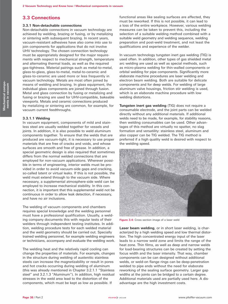
www.pfeiffer-vacuum.comPage 38 / Part 2
2 Vacuum Technology and Know how / Mechanical components in vacuumM
ech
anic
al c
om
po-
nen
ts in
vac
uu
m
3.3 Connections
3.3.1 Non-detachable connectionsNon-detachable connections in vacuum technology are achieved by welding, brazing or fusing, or by metalizing or sintering with subsequent brazing. In recent years, vacuum-resistant adhesives have also come into use to join components for applications that do not involve UHV technology. The chosen connection technology must be appropriately designed for the major require-ments with respect to mechanical strength, temperature and alternating thermal loads, as well as the required gas-tightness. Material pairings such as metal-to-metal, glass-to-glass, glass-to-metal, metal-to-ceramic and glass-to-ceramic are used more or less frequently in vacuum technology. Metals are most often joined by means of welding and brazing. In glass equipment, the individual glass components are joined through fusion. Metal and glass connection by fusing or metalizing and fusing or brazing are used for UHV-compatible, bakeable viewports. Metals and ceramic connections produced by metalizing or sintering are common, for example, for vacuum current feedthroughs.
3.3.1.1 WeldingIn vacuum equipment, components of mild and stain-less steel are usually welded together for vessels and joints. In addition, it is also possible to weld aluminum components together. To ensure that the welds that are produced are vacuum-tight, it is necessary to use proper materials that are free of cracks and voids, and whose surfaces are smooth and free of grease. In addition, a special geometric design is also required that sometimes differs from the normal welded connections that are employed for non-vacuum applications. Wherever possi-ble in terms of engineering, interior welds must be pro-vided in order to avoid vacuum-side gaps and cracking, so-called latent or virtual leaks. If this is not possible, the weld must extend through to the vacuum side. Where necessary, a supplemental atmosphere-side weld can be employed to increase mechanical stability. In this con-nection, it is important that this supplemental weld not be continuous in order to allow leak detection, if necessary, and have no air inclusions.
The welding of vacuum components and chambers requires special knowledge and the welding personnel must have a professional qualification. Usually, a weld-ing company documents this with regular tests of their welders through independent testing institutes. In addi-tion, welding procedure tests for each welded material and the weld geometry should be carried out. Specially trained welding personnel, for example welding engineers or technicians, accompany and evaluate the welding work.
The welding heat and the relatively rapid cooling can change the properties of materials. For example, changes in the structure during welding of austenitic stainless steels can increase the magnetizability or result in pores and hot cracks occurring during welding of aluminum (this was already mentioned in Chapter 3.2.1.1 “Stainless steel” and 3.2.1.3 “Aluminum”). In addition, high residual stresses in the weld area lead to the distortion of the components, which must be kept as low as possible. If
functional areas like sealing surfaces are affected, they must be reworked. If this is not possible, it can lead to a loss of the entire workpiece. However, various welding measures can be taken to prevent this, including the selection of a suitable welding method combined with a suitable weld geometry and welding sequence, welding preparation and post-weld treatment, and not least the qualifications and experience of the welder.
In vacuum technology tungsten inert gas welding (TIG) is used often. In addition, other types of gas shielded metal arc welding are used as well as special methods, such as micro-plasma welding for thin-walled components or orbital welding for pipe components. Significantly more elaborate machine procedures are laser welding and electron beam welding. Both are suitable for delicate components and for deep welds. For welding of large aluminum valve housings, friction stir welding is used, which is an elaborate machine procedure with low welding distortions.
Tungsten inert gas welding (TIG) does not require a consumable electrode, and the joint parts can be welded directly without any additional materials. If additional welds need to be made, for example, for stability reasons, then welding consumables can be used. Other advan-tages of this method are virtually no spatter, no slag formation and versatility: stainless steel, aluminum and also copper can be TIG welded. The TIG method is preferred if a high quality weld is desired with respect to the welding speed.
Figure 3.4: Cross section image of a laser weld
Laser beam welding, or in short laser welding, is char-acterized by a high welding speed and low thermal distor-tion. The high concentrated energy input of the laser leads to a narrow weld zone and limits the range of the heat zone. Thin films, as well as deep and narrow welds for load-bearing structures can be created by setting the focus width and the laser intensity. That way, chamber components can be can designed without additional welds, or weld-on flange rings can be deep-penetration welded to pipe ends without the need for elaborate reworking of the sealing surface geometry. Larger gap widths at the joints can be bridged to a certain degree. Additional materials used are partially used here. A dis-advantage are the high investment costs.

www.pfeiffer-vacuum.com Part 2 / Page 39
2 Vacuum Technology and Know how / Mechanical components in vacuum
Mec
han
ical
com
po-
nen
ts in
vac
uu
m
Figure 3.5: Cross section image of WIG orbital weld
Orbital welding is a fully mechanized inert gas welding process that provides steady high seam quality, as the arc is lead mechanically and under controlled conditions around the pipes or the round component. The system expense is higher than for TIG welding. An orbital welding tong covers only a limited range of pipe diameters. Each tube outside diameter also requires a device suitable for holding the pipe.
During electron beam welding, accelerated, focused electrons provide the energy required in the weld zone. In order to prevent the scattering and absorption of the electrons, the process is carried out in a high vacuum. This also makes it possible to weld highly reactive mate-rials. The high system price and the weld preparation with possibly a required equipment construction, it usu-ally leads to high prices for the procedure and mainly restricts its use to series components.
After the welding of austenitic stainless steel a metalli-cally smooth surface must be present again, so an even chromium oxide passive layer without interruptions can be formed. For example, an inert gas shielding (including for the root base) prevents scaling of the surface at tem-peratures above 600°C. Mechanical or chemical finishing followed by thorough rinsing removes discoloration on the surface and cleans the component.
3.3.1.2 Brazing, fusing and metallizationIn addition to welding, the soldering process is also used to join metals. Soldered joints at soldering temperatures of above 600 °C are used almost exclusively in vacuum technology. In order to eliminate the need for highly cor-rosive flux when soldering, which often involves high vapor pressure, and in order to obtain oxide-free, high-strength joints, the soldering process is performed under vacuum or in a clean inert gas atmosphere. Soft solder joints are often not suitable for vacuum applications. They typically cannot be baked out, have less mechani-cal strength and in addition to tin, which has a low vapor pressure, frequently contain other alloy components with a high vapor pressure. Analogously to vacuum welds, a vacuum- brazed connection occurs when the following requirements in particular are met: carefully cleaned surfaces, careful formation of the soldering gap, use of a gas-free solder with a low vapor pressure, good flow and wetting properties of the solder (gap filling), a well-defined fusion zone of the solder and low reaction between the soldering and the base material. The stan-dard brazing alloys can be divided into two major groups: Brazing alloys based on noble metals (mainly
silver) and nickel-based brazing alloys. The structured noble metal-based low-melting brazing alloys are signifi-cantly more expensive than the higher-melting nickel base. Therefore, it is preferable to use nickel-base alloys, if this is technically possible and if a higher processing temperature is acceptable. The arrangement of the com-ponents to each other and the solder gaps between them must match the soldering process. Depending on the nature of the solder used, the soldering temperature and the thermal expansion of the components, the solder gaps (at room temperature) are typically 0.03 to 0.1 mm. The question of when welding and when brazing should be used, cannot be answered in a general and comprehensive way. Except in cases where welding is not possible, brazing can be advantageous if as many connecting points as possible can be produced simulta-neously in a batch.
The fusing process is primarily used for glass equipment and for glass-to-metal connections. Glass-to-metal fus-ings are especially important in the production of vacuum-tight current feedthroughs, for bakeable viewports and in the production of vacuum gauges. To fuse glass-to-metal transitions, the materials must be selected in such a manner that the thermal expansion coefficients of these materials are as similar to one another as possible throughout a broad temperature range. Since this is often not the case, numerous special alloys have been developed for so-called non-adapted glass-metal seals. In the form of a welded lip, they provide an elastic contact between glass and stainless steel for viewports. Fusings are difficult to perform with quartz glass, as it has a very low thermal expansion, which metal and metal alloys can nowhere near achieve.
Ceramic-to-metal connections are used for highly bake-able and highly insulating current feedthroughs. These are used among other things for the production of high-performance transmitting tubes and ceramic vacuum chambers for particle accelerator of the physical large-scale research. Connections with ceramic, e.g. aluminum oxide (92 % to 98 % Al203), are pre-metalized with those points to be joined with the metal. In this connection, it is particularly important to ensure that the thin metal layer (molybdenum or titanium) creates a thorough connection, free of voids and pores, with the ceramic substrate. For the production of electrical feedthroughs. a nickel layer is applied subsequently, to which a metal cap is brazed and a conductor is then soldered to.
3.3.2 Detachable flange connectionsThe individual components of a vacuum system, e.g. vacuum chambers, pumps, valves, measurement instru-ments, etc., are connected with one another either directly or by means of pipe components or resilient ele-ments. The detachable interfaces between the compo-nents must be vacuum-tight. In configuring a vacuum system, however, as few detachable joints as possible should be used, as they represent a significantly more frequent source of potential leakage than non-detachable joints.
Flange components from stainless steel, aluminum and steel can be used as connection elements. Metal hoses

www.pfeiffer-vacuum.comPage 40 / Part 2
2 Vacuum Technology and Know how / Mechanical components in vacuumM
ech
anic
al c
om
po-
nen
ts in
vac
uu
m
made of stainless steel are preferable to thick-walled rubber or thermoplastics for flexible joints. They are a strict necessity from the lower medium vacuum range onward.
From low to high vacuum ranges, ISO-KF flange con-nections with nominal widths of DN 10 to DN 50 are used for detachable connections, for larger nominal sizes of DN 63 to DN 1000 ISO-K and ISO-F flanges are used. Ultra-high vacuum compatible releasable connec-tion, are in nominal widths DN 16 to DN 400 as a CF flange connection, respectively for larger nominal diam-eters of DN 400 to DN 800 flanges as a COF flange.
3.3.2.1 O-ring seals and grooves When vacuum technology components are detachably joined, seals must be used to prevent ambient air from flowing into the vacuum. To prevent this, there are, depending on the application and pressure range differ-ent types of seals.
O-rings are the most frequently used of all seals. They are available in different materials, usually elastomers with a hardness in the range of 65 to 80 Shore A. The unit Shore A is used for soft elastomers as a measure of malleability. The higher the number, the lower the defor-mation with the same applied force. The suitability of O-rings as good vacuum seals stems from their ability to adapt to the minute unevenness of the mating sur-faces. The surface of the O-ring must be free of releas-ing grease or talcum, smooth and crack-free and scratch-free. The rings should be seamlessly pressed, the parting of the pressing tool should be on the level of the ring diameter and can be removed by grinding.
The O-ring can be coated with a thin film of a low vapor pressure grease (silicon grease, mineral oil-based or perfluoropolyether-based grease), depending upon the application in question. The vacuum grease smooth out small irregularities on the sealing surfaces and the surface of the O-ring and thereby improves, particularly at low degrees of deformation, the sealing effect. Here, the vapor pressure of the grease should be noted increases greatly with the temperature and should be well below the desired operating pressure. In addition, it must be examined whether components of the grease or low amounts of hydrocarbons are compatible with the application. In the case of dry installation, particular attention must be paid to surface quality, the cleanli-ness of the mating surfaces as well as to the sealing material. In addition, the degree of deformation should not be too small, to ensure good contact between the O-ring and sealing surfaces.
The cord diameter of the O-rings is usually 2 to 12 mm. The diameter for many connections is 5 mm resp. 5.33 mm in the area of the inch dimension. Generally speaking, O-rings are used as static seals. If dynamic stress is involved, precision O-rings that are manufactured especially for this purpose or alternatively mechanical seals or radial shaft seal rings, should be used.
O-rings can also be used in axial or radial grooves, in addition to being employed in conjunction with centering rings or sealing washers. In most cases, O-rings are
placed in grooves and pressed between flanges, by gen-erally using a combination of one flat flange and one grooved flange. The grooves must be carefully dimen-sioned. There are no generally accepted dimensions for this. The dimensions listed in the tables of O-ring suppli-ers are only reference values are used for orientation. They must be checked by the user on each specific application and suitability (e.g. through tests). Elastomers swell, shrink, harden or can even crack, due to external influences, such as temperature, pressure or reactions with the fluids used. This must be considered when selecting the elastomer and the groove. In addition, the sealing effect must be sufficient during each operating condition to ensure that the O-ring is not excessively compressed. If due to an increase in volume of the O-ring the groove is overfilled, it can damage the O-ring or even distort the flange.
For static sealing the maximum compression for a cord thickness of 5 mm should be about 25 %. Smaller diame-ters can be compressed more, larger diameters less. In practice, a compression of less than 15 %, in particular for dry mounting, can cause an insufficient sealing effect. The deformation force is mainly determined by the cord thickness and the hardness of the elastomer. To compress an O-ring of 5.33 mm thickness by 20 %, approx 5 N per mm of sealing length is required for a hardness of 70 Shore A resp. 7 N/mm for 80 Shore A.
To facilitate assembly, the diameter of the O-ring groove is usually selected somewhat larger than the diameter of the O-ring. This keeps the O-ring in the groove during assembly. Elastomer rings can safely be stretched in length by 5 %. The maximum stretch is dependent on the material and the operating conditions.
Elastomeric seals with trapezoidal or similar cross-sec-tions can be used, for example, for valve seats and for lids and doors of vacuum chambers. The trapezoidal opening should be dimensioned such that the O-ring is not damaged when inserted and on the other hand is not pulled out when the valve plate is lifted or when you open the chamber door. In addition, with large contact forces, as they occur e.g. for large chamber doors, the trapezoidal-groove must allow enough room for the deformed O-ring, so that its deformation is kept within limits.
To seal screws, e. g. oil filler screws or oil drain plugs, the O-ring is installed in an angular position. The thread has a chamfer of 45 ° at the upper end, into which the O-ring is inserted and then compressed by the surface of the screw. The seal should be lubricated, so it is not damaged during tightening. In addition, the installation space must be greater than the volume of the O-ring.
Flat gaskets in combination with planar sealing surfaces are to be avoided in vacuum technology as much as possible. For this, a hard to reach high contact force is required, so that the sealing material fills any surface irregularities. If flat gaskets are used, this usually happens with circulating locally raised sealing surfaces, for example, with the combination of CF flange with a FKM flat gasket.

www.pfeiffer-vacuum.com Part 2 / Page 41
2 Vacuum Technology and Know how / Mechanical components in vacuum
Mec
han
ical
com
po-
nen
ts in
vac
uu
m
3.3.2.2 ISO-KF flangeISO-KF small flange components are described in DIN 28403 and ISO 2861 in nominal diameters DN 10 to DN 50. The connections suitable for pressures up to 1 · 10-8 hPa and can be used for overpressures up to 1,500 hPa. With metal seals, the pressure range can be extended to less than 1 · 10-9 hPa. The significantly higher contact pressures required for this are created with special clamps for metal seals.
An ISO-KF connection consists of two symmetrical flanges and one O-ring seal, which is positioned and supported with an internal or external centering ring (Figure 3.7). The necessary pressing force for the sealing is created by a clamping ring, which is placed over the conical tightening area and is tightened with a wing screw. This allows for a fast, efficient assembly and disassembly without any tools. The flanges can be aligned around its main axis in any direction.
For mounting a KF flange on a base plate, (Figure 3.8) claw clamps or bulkhead clamps are used as clamping elements. The dimensions of the bores in the base plate can be found in the product description of the claws and bulkhead clamps.
Figure 3.7: ISO-KF connection with centering ring and clamping ring
Figure 3.8: ISO-KF flange mounted on base plate with centering ring and claw clamps
Figure 3.6: O-ring seals in rectangular groove, trapezoidal-groove and in an angular position
groo
ve d
epth
groove width
groo
ve d
epth
opening angle
groove width

www.pfeiffer-vacuum.comPage 42 / Part 2
2 Vacuum Technology and Know how / Mechanical components in vacuumM
ech
anic
al c
om
po-
nen
ts in
vac
uu
m
3.3.2.3 ISO-K/ISO-F flangeISO-K clamping flange components and ISO-F fixed flange components are described in DIN 28404 and ISO 1609 in nominal diameters DN 10 to DN 630 for ISO-K flanges and to DN 1000 for ISO-F flanges. The connections are suitable for pressures up to 1 · 10-8 hPa and can be used for overpressures up to 1,500 hPa. With metal seals, the pressure range can be extended to less than 1 · 10-9 hPa. Metal seals require significantly higher contact forces. Screwed flange connections provide that. If clamp screws are used, their number must be increased if necessary.
An ISO-K and ISO-F compound consists of two symmet-rical flanges and one O-ring seal, which is positioned and supported with an inner centering ring and also sup-ported by an outer ring. The required contact pressure for sealing, is created with double claw clamps (Figure 3.9) or screws (Figure 3-13).
With ISO-K flanges, a circumferential outer ridge on the back of the flanges prevents slippage by the clamp screws. The flanges can be aligned around the main axis in any direction. Claw clamps are used for mounting an ISO K flange on a base plate. Depending on whether a centering ring is resting on the base plate (Figure 3.10) or an O-ring lies in base plate (Figure 3.11), claw clamps of different heights are used. Alternatively, the ISO-K flange can be screwed with a bolt ring onto the base plate (Figure 3.12).
The ISO-F flange has a fixed bolt hole circle that is dependent on the nominal diameter. The flanges can be aligned with a hole spacing around the main hole axis. An ISO-F flange can be bolted onto a base plate. As a seal, a centering ring can be used or an O-ring with a sealing groove in the base plate.
Mounting an ISO-K flange on to an ISO-F flange can be done with a bolt ring (Figure 3.14). To install the bolt ring, it is slipped over the ISO-K flange and then a circlip is put into the outer circumferential groove of the ISO-K flange. The flanges can be aligned around the main axis in any direction.
Figure 3.10: ISO-K flange mounted on base plate with centering ring and claw clamps
Figure 3.11: ISO-K flange mounted on base plate with O-ring nut and claw clamps for base plate with sealing groove
Figure 3.12: ISO-K flange mounted on base plate with centering ring, bolt ring and screws
Figure 3.9: ISO-K connection with centering ring and double claw clamps
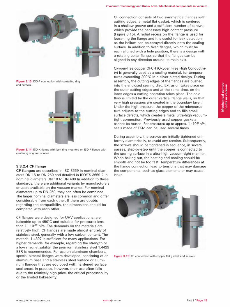
www.pfeiffer-vacuum.com Part 2 / Page 43
2 Vacuum Technology and Know how / Mechanical components in vacuum
Mec
han
ical
com
po-
nen
ts in
vac
uu
m
3.3.2.4 CF flangeCF flanges are described in ISO 3669 in nominal diam-eters DN 16 to DN 250 and detailed in ISO/TS 3669-2 in nominal diameters DN 10 to DN 400 In addition to these standards, there are additional variants by manufacturers or users available on the vacuum market. For nominal diameters up to DN 250, they can often be combined. The larger nominal diameters are less common and differ considerably from each other. If there are doubts regarding the compatibility, the dimensions should be compared with each other.
CF flanges were designed for UHV applications, are bakeable up to 450°C and suitable for pressures less than 1 · 10-12 hPa. The demands on the materials are relatively high. CF flanges are made almost entirely of stainless steel, generally with a low carbon content. The material 1.4307 is sufficient for many applications. For higher demands, for example, regarding the strength or a low magnetizability, the premium stainless steel 1.4429 ESR is recommended. For use on aluminum chambers, special bimetal flanges were developed, consisting of an aluminum base and a stainless steel surface or alumi-num flanges that are equipped with hardened surface seal areas. In practice, however, their use often fails due to the relatively high price, the critical processability or the limited bakeability.
CF connection consists of two symmetrical flanges with cutting edges, a metal flat gasket, which is centered in a shallow groove and a sufficient number of screws, which provide the necessary high contact pressure (Figure 3.15). A radial recess on the flange is used for loosening the flange and it is useful for leak detection, as the helium can be sprayed directly onto the sealing surface. In addition to fixed flanges, which must be each aligned with a hole position, there is a design with a rotating collar flange, so that the flanges can be aligned in any direction around its main axis.
Oxygen-free copper OFCH (Oxygen Free High Conductivi-ty) is generally used as a sealing material, for tempera-tures exceeding 200°C in a silver plated design. During assembly, the cutting edges of the flanges are pushed into the enclosed sealing disc. Extrusion takes place on the outer cutting edges and at the same time, on the inner edges a cutting operation takes place. The cold flow is limited by the outer vertical flange walls, so that very high pressures are created in the boundary layer. Under the high pressure, the copper of the microstruc-ture adjusts to the cutting edges and to fills small surface defects, which creates a metal ultra-high vacuum-tight connection. Previously used copper gaskets cannot be reused. For pressures up to approx. 1 · 10-8 hPa, seals made of FKM can be used several times.
During assembly, the screws are initially tightened uni-formly diametrically, to avoid any tension. Subsequently, the screws should be tightened in sequence, in several passes, step-by-step until the copper is connected to the sealing surface in a ultra-high vacuum-tight manner. When baking out, the heating and cooling should be smooth and not be too fast. Temperature differences at the flange connection lead to tensions that may damage the components, such as glass elements or may cause leaks.
Figure 3.14: ISO-K flange with bolt ring mounted on ISO-F flange with centering ring and screws
Figure 3.15 CF connection with copper flat gasket and screws
Figure 3.13: ISO-F connection with centering ring and screws
:
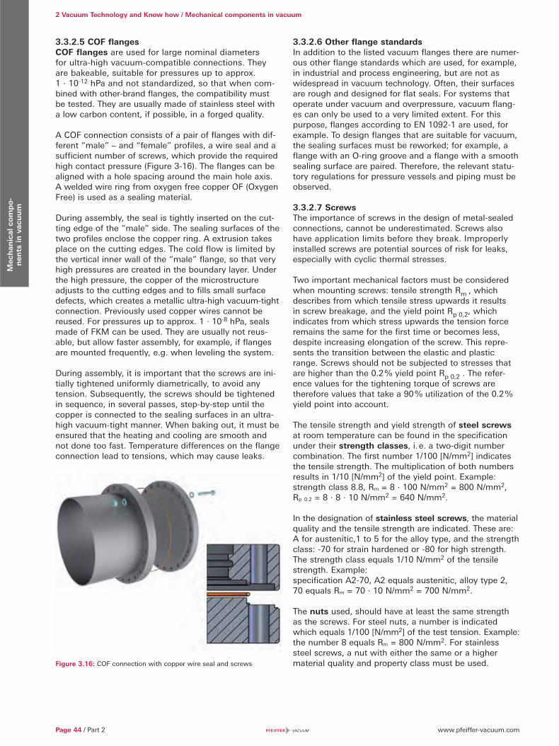
www.pfeiffer-vacuum.comPage 44 / Part 2
2 Vacuum Technology and Know how / Mechanical components in vacuumM
ech
anic
al c
om
po-
nen
ts in
vac
uu
m
3.3.2.5 COF flangesCOF flanges are used for large nominal diameters for ultra-high vacuum-compatible connections. They are bakeable, suitable for pressures up to approx. 1 · 10-12 hPa and not standardized, so that when com-bined with other-brand flanges, the compatibility must be tested. They are usually made of stainless steel with a low carbon content, if possible, in a forged quality.
A COF connection consists of a pair of flanges with dif-ferent “male” – and “female” profiles, a wire seal and a sufficient number of screws, which provide the required high contact pressure (Figure 3-16). The flanges can be aligned with a hole spacing around the main hole axis. A welded wire ring from oxygen free copper OF (Oxygen Free) is used as a sealing material.
During assembly, the seal is tightly inserted on the cut-ting edge of the “male” side. The sealing surfaces of the two profiles enclose the copper ring. A extrusion takes place on the cutting edges. The cold flow is limited by the vertical inner wall of the “male” flange, so that very high pressures are created in the boundary layer. Under the high pressure, the copper of the microstructure adjusts to the cutting edges and to fills small surface defects, which creates a metallic ultra-high vacuum-tight connection. Previously used copper wires cannot be reused. For pressures up to approx. 1 · 10-8 hPa, seals made of FKM can be used. They are usually not reus-able, but allow faster assembly, for example, if flanges are mounted frequently, e.g. when leveling the system.
During assembly, it is important that the screws are ini-tially tightened uniformly diametrically, to avoid any tension. Subsequently, the screws should be tightened in sequence, in several passes, step-by-step until the copper is connected to the sealing surfaces in an ultra-high vacuum-tight manner. When baking out, it must be ensured that the heating and cooling are smooth and not done too fast. Temperature differences on the flange connection lead to tensions, which may cause leaks.
Figure 3.16: COF connection with copper wire seal and screws
3.3.2.6 Other flange standards In addition to the listed vacuum flanges there are numer-ous other flange standards which are used, for example, in industrial and process engineering, but are not as widespread in vacuum technology. Often, their surfaces are rough and designed for flat seals. For systems that operate under vacuum and overpressure, vacuum flang-es can only be used to a very limited extent. For this purpose, flanges according to EN 1092-1 are used, for example. To design flanges that are suitable for vacuum, the sealing surfaces must be reworked; for example, a flange with an O-ring groove and a flange with a smooth sealing surface are paired. Therefore, the relevant statu-tory regulations for pressure vessels and piping must be observed.
3.3.2.7 ScrewsThe importance of screws in the design of metal-sealed connections, cannot be underestimated. Screws also have application limits before they break. Improperly installed screws are potential sources of risk for leaks, especially with cyclic thermal stresses.
Two important mechanical factors must be considered when mounting screws: tensile strength Rm , which describes from which tensile stress upwards it results in screw breakage, and the yield point Rp 0,2, which indicates from which stress upwards the tension force remains the same for the first time or becomes less, despite increasing elongation of the screw. This repre-sents the transition between the elastic and plastic range. Screws should not be subjected to stresses that are higher than the 0.2 % yield point Rp 0,2 . The refer-ence values for the tightening torque of screws are therefore values that take a 90 % utilization of the 0.2 % yield point into account.
The tensile strength and yield strength of steel screws at room temperature can be found in the specification under their strength classes, i. e. a two-digit number combination. The first number 1/100 [N/mm2] indicates the tensile strength. The multiplication of both numbers results in 1/10 [N/mm2] of the yield point. Example: strength class 8.8, Rm = 8 · 100 N/mm2 = 800 N/mm2, Rp 0.2 = 8 · 8 · 10 N/mm2 = 640 N/mm2.
In the designation of stainless steel screws, the material quality and the tensile strength are indicated. These are: A for austenitic,1 to 5 for the alloy type, and the strength class: -70 for strain hardened or -80 for high strength. The strength class equals 1/10 N/mm2 of the tensile strength. Example: specification A2-70, A2 equals austenitic, alloy type 2, 70 equals Rm = 70 · 10 N/mm2 = 700 N/mm2.
The nuts used, should have at least the same strength as the screws. For steel nuts, a number is indicated which equals 1/100 [N/mm2] of the test tension. Example: the number 8 equals Rm = 800 N/mm2. For stainless steel screws, a nut with either the same or a higher material quality and property class must be used.
www.pfeiffer-vacuum.com Part 2 / Page 45
2 Vacuum Technology and Know how / Mechanical components in vacuum
Mec
han
ical
com
po-
nen
ts in
vac
uu
m
Caution: nuts, with a lower height than 0.8 times the screw diameter (flat design), have a restricted load- bearing capacity.
Type of screw 0.2% yield pointRp 0.2 [N/mm2]
Tensile strengthRm [N/mm2]
Material
Stainless steel, A2-70
450 700 Stainless steel, 1.4301, 1.4303, 1.4307
Stainless steel, A4-80
600 800 Stainless steel 1.4401
Steel, strength class 8.8
640 800 Carbon steel, quenched and tempered
Table 3.6: Mechanical characteristics and material of screws at room temperature
To determine the tightening torque and the preload stress, it is necessary to know the friction coefficient μtotal of the screw connection. Due to the variety of surfaces and lubrication conditions, it is impossible to provide reliable values . The scattering is too large. For this reason, only scattering ranges for the friction coefficient can be provided. To determine the correct torque, a test under operating conditions is recommended.
The friction coefficients can be reduced by the use of lubricants, however, the large scattering range remains the same. It should be noted that a smaller friction coefficient leads to a lower maximum torque. Hence: Use of lubricants friction coefficient μtotal drops less torque is necessary or may be applied.
For stainless steel screws, the friction values in the thread and on the supporting surfaces are substantially greater than with tempered steel screws. The scattering ranges of the friction values is also much larger (up to above 100 %). Due to the high edge pressure, they also tend to get stuck. A lubricant can generally help in this case. Alternatively, silver plated screws or nuts can be used.
Screw Nut μtotal with out lubrica-tion
μtotal with MoS2 paste
μtotal greased
A2 or A4 A2 or A4 0.23 – 0.50 0.10 – 0.20 –
Steel, electrolyti-cally galvanized
Steel, electrolyti-cally galvanized
0.12 – 0.20 – 0.10 – 0.18
Table 3.7: Friction coefficient for stainless steel and zinc-plated steel screws
Properties of screws at elevated temperaturesWhen using screws at elevated temperatures, it must be noted that the tensile strength and yield point are reduced. In addition, the creep strain or heat resistance must be considered as a basis for assessing the mechanical strength. Therefore, information on yield strength serves only as a guide. For critical or safety-related applications and other mechanical parameters and all influencing factors must be considered.
Type of screw 0.2% yield point Rp 0,2 [N/mm2] at
20°C 100 °C 200 °C 300 °C 400 °C
Stainless steel, A2-70
450 380 360 335 315
Stainless steel, A4-80
600 510 480 450 420
Steel, strength class 8.8
640 590 540 480 –
Table 3.8: Temperature dependence of the 0.2% yield point for stainless steel and steel screws with diameters ≤ M24
If a through-hole screw connection is tightened by the rotation of the nut, a tensile force is created in the threaded bolt and an equal compressive force between the plates. As a result, the screw is elongated and the component compressed. Through the elongation of the screw, the preload stress is created. The clamping force is produced by the compression of the parts, and with-out any additional force on the connection is the same size as the preload force.
During tightening of the screw, friction between the con-tact surfaces is created. With a growing preload force, the friction moments in the thread and the nut contact area increase. The maximum preload force represents the sum of the friction moments the majority of the total tightening torques. With lubricated screws (small friction coefficients) the friction proportion is lower, so that the screws produce a higher preload stress with the same tightening torque. It should be noted that the maximum permissible tightening torque with lubricated screws is lower than with non-lubricated screws.
Preload force and torque cause tensile and torsional stresses in the screw. Both influences must be simulta-neously considered during the calculation of the screw load . An alternative for the calculation are tables, as they appear in the VDI guideline 2230. If a 90 % utiliza-tion of the 0.2 % yield point is considered acceptable, the maximum permissible tightening torque and the associated preload stresses for the different friction coef-ficients can be found there. However, the information only represents non-binding values for guidance. For critical or safety-related applications, all influencing fac-tors that may be required for a screws calculation must be considered. Excerpts from the tables for stainless steel and steel screws are listed below.

www.pfeiffer-vacuum.comPage 46 / Part 2
2 Vacuum Technology and Know how / Mechanical components in vacuumM
ech
anic
al c
om
po-
nen
ts in
vac
uu
m
If screws are screwed into blind holes, an enclosed hollow space is created at the end of the threaded hole. Such dead volume is drained under vacuum only very slowly and leads to prolonged outgassing, which mani-fests itself in the same way as a leak. It is therefore also called a virtual leak. Under high vacuum and particularly UHV conditions, dead volume of this type should be constructively avoided or if that is not possible, it must be vented.
Dimension and quality
Max. tightening torque [Nm] for μtotal = Max. preload force [km] for μtotal =
0.10 0.14 0.20 0.30 0.40 0.10 0.14 0.20 0.30 0.40
M4, A2-70M4, A4-80
1.72.3
2.22.9
2.63.5
3.04.1
3.34.4
2.973.96
2.733.64
2.403.20
1.942.59
1.602.13
M5, A2-70M5, A4-80
3.44.6
4.25.6
5.16.9
6.18.0
6.68.8
4.856.47
4.475.96
3.935.24
3.194.25
2.623.50
M6, A2-70M6, A4-80
5.98.0
7.49.9
8.811.8
10.413.9
11.315.0
6.859.13
6.318.41
5.547.39
4.495.98
3.704.93
M8, A2-70M8, A4-80
14.519.3
17.823.8
21.528.7
25.533.9
27.636.8
12.616.7
11.615.4
10.213.6
8.2511.0
6.809.10
M10, A2-70M10, A4-80
30.039.4
36.047.8
44.058.0
51.069.0
56.075.0
20.026.5
18.424.8
16.221.7
13.117.5
10.814.4
M12, A2-70M12, A4-80
5067
6282
74100
88117
96128
29.138.8
26.935.9
23.731.5
19.225.6
15.821.1
M16, A2-70M16, A4-80
121161
150198
183245
218291
237316
55.073.3
50.967.9
44.959.8
36.448.6
30.040.0
All data are approximate values for room temperature – see VDI 2230.For hexagon screws (ISO 4014 and 4017), hexagon socket screws (ISO 4762) and nuts (ISO 4032) with standard thread at a 90 % utilization of the 0.2 % yield point Rp 0.2.
Table 3.9: Maximum tightening torque and maximum resulting preload force for stainless steel screws
Dimension and strength class
Max. tightening torque [Nm] Max. preload force [kN] for μtotal =
0.10 0.12 0.14 0.10 0.12 0.14
M4, 8.8 2.6 3.0 3.3 4.5 4.4 4.3
M5, 8.8 5.2 5.9 6.5 7.4 7.2 7.0
M6, 8.8 9.0 10.1 11.3 10.4 10.2 9.9
M8, 8.8 21.6 24.6 27.3 19.1 18.8 18.1
M10, 8.8 43 48 54 30.3 29.6 28.8
M12, 8.8 73 84 93 44.1 43.0 41.9
M16, 8.8 180 206 230 82.9 80.9 78.8
All data are approximate values for room temperature - see VDI 2230. For hexagon screws (ISO 4014 and 4017), hexagon socket screws (ISO 4762) and nuts (ISO 4032) with standard thread at a 90% utilization of the 0.2% yield point Rp 0.2.
Table 3.10: Maximum tightening torque and maximum resulting preload force for steel screws of strength class 8.8
An alternative are vacuum screws which offer a com-fortable means of venting. Their core has drilled holes (degassing bores). The screw head area has also a radial milling groove (degassing reduction), through which the area of the feedthrough hole of the screw connection is vented. The mechanical parameters for screws are not applicable to vacuum screws, as the vent hole leads to mechanical weakening.
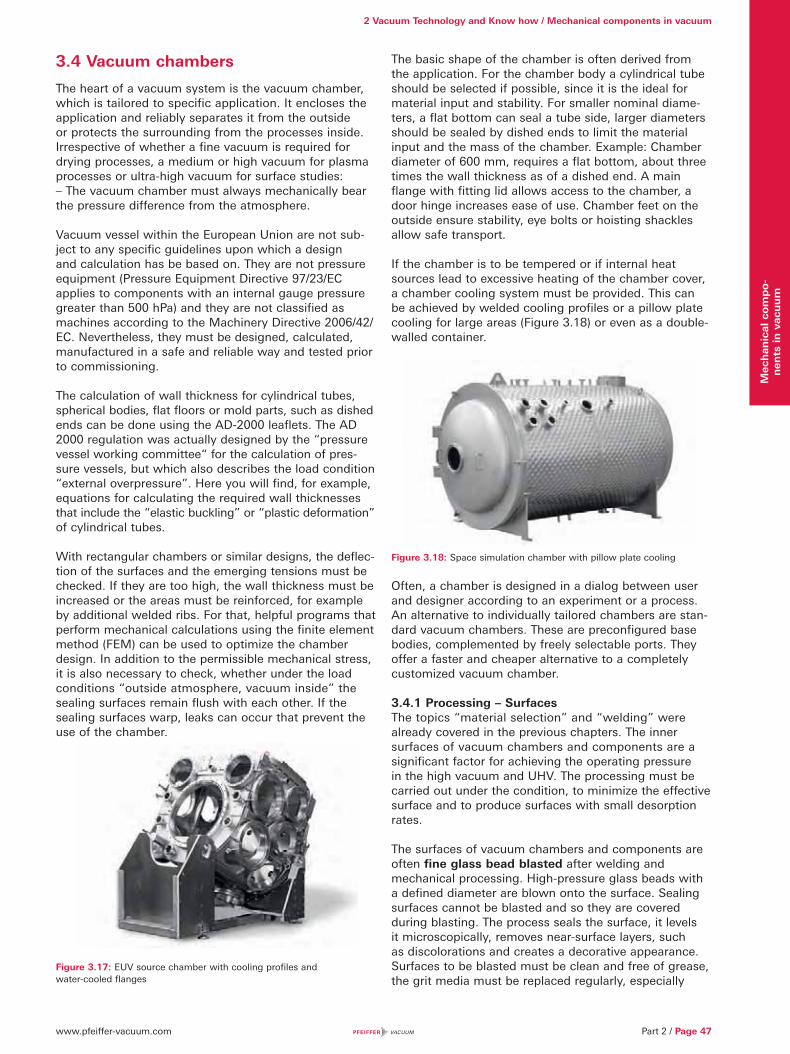
www.pfeiffer-vacuum.com Part 2 / Page 47
2 Vacuum Technology and Know how / Mechanical components in vacuum
Mec
han
ical
com
po-
nen
ts in
vac
uu
m
3.4 Vacuum chambers
The heart of a vacuum system is the vacuum chamber, which is tailored to specific application. It encloses the application and reliably separates it from the outside or protects the surrounding from the processes inside. Irrespective of whether a fine vacuum is required for drying processes, a medium or high vacuum for plasma processes or ultra-high vacuum for surface studies: – The vacuum chamber must always mechanically bear the pressure difference from the atmosphere.
Vacuum vessel within the European Union are not sub-ject to any specific guidelines upon which a design and calculation has be based on. They are not pressure equipment (Pressure Equipment Directive 97/23/EC applies to components with an internal gauge pressure greater than 500 hPa) and they are not classified as machines according to the Machinery Directive 2006/42/EC. Nevertheless, they must be designed, calculated, manufactured in a safe and reliable way and tested prior to commissioning.
The calculation of wall thickness for cylindrical tubes, spherical bodies, flat floors or mold parts, such as dished ends can be done using the AD-2000 leaflets. The AD 2000 regulation was actually designed by the “pressure vessel working committee“ for the calculation of pres-sure vessels, but which also describes the load condition “external overpressure”. Here you will find, for example, equations for calculating the required wall thicknesses that include the “elastic buckling” or “plastic deformation” of cylindrical tubes.
With rectangular chambers or similar designs, the deflec-tion of the surfaces and the emerging tensions must be checked. If they are too high, the wall thickness must be increased or the areas must be reinforced, for example by additional welded ribs. For that, helpful programs that perform mechanical calculations using the finite element method (FEM) can be used to optimize the chamber design. In addition to the permissible mechanical stress, it is also necessary to check, whether under the load conditions “outside atmosphere, vacuum inside” the sealing surfaces remain flush with each other. If the sealing surfaces warp, leaks can occur that prevent the use of the chamber.
Figure 3.17: EUV source chamber with cooling profiles and water-cooled flanges
The basic shape of the chamber is often derived from the application. For the chamber body a cylindrical tube should be selected if possible, since it is the ideal for material input and stability. For smaller nominal diame-ters, a flat bottom can seal a tube side, larger diameters should be sealed by dished ends to limit the material input and the mass of the chamber. Example: Chamber diameter of 600 mm, requires a flat bottom, about three times the wall thickness as of a dished end. A main flange with fitting lid allows access to the chamber, a door hinge increases ease of use. Chamber feet on the outside ensure stability, eye bolts or hoisting shackles allow safe transport.
If the chamber is to be tempered or if internal heat sources lead to excessive heating of the chamber cover, a chamber cooling system must be provided. This can be achieved by welded cooling profiles or a pillow plate cooling for large areas (Figure 3.18) or even as a double-walled container.
Figure 3.18: Space simulation chamber with pillow plate cooling
Often, a chamber is designed in a dialog between user and designer according to an experiment or a process. An alternative to individually tailored chambers are stan-dard vacuum chambers. These are preconfigured base bodies, complemented by freely selectable ports. They offer a faster and cheaper alternative to a completely customized vacuum chamber.
3.4.1 Processing – SurfacesThe topics “material selection” and “welding” were already covered in the previous chapters. The inner surfaces of vacuum chambers and components are a significant factor for achieving the operating pressure in the high vacuum and UHV. The processing must be carried out under the condition, to minimize the effective surface and to produce surfaces with small desorption rates.
The surfaces of vacuum chambers and components are often fine glass bead blasted after welding and mechanical processing. High-pressure glass beads with a defined diameter are blown onto the surface. Sealing surfaces cannot be blasted and so they are covered during blasting. The process seals the surface, it levels it microscopically, removes near-surface layers, such as discolorations and creates a decorative appearance. Surfaces to be blasted must be clean and free of grease, the grit media must be replaced regularly, especially
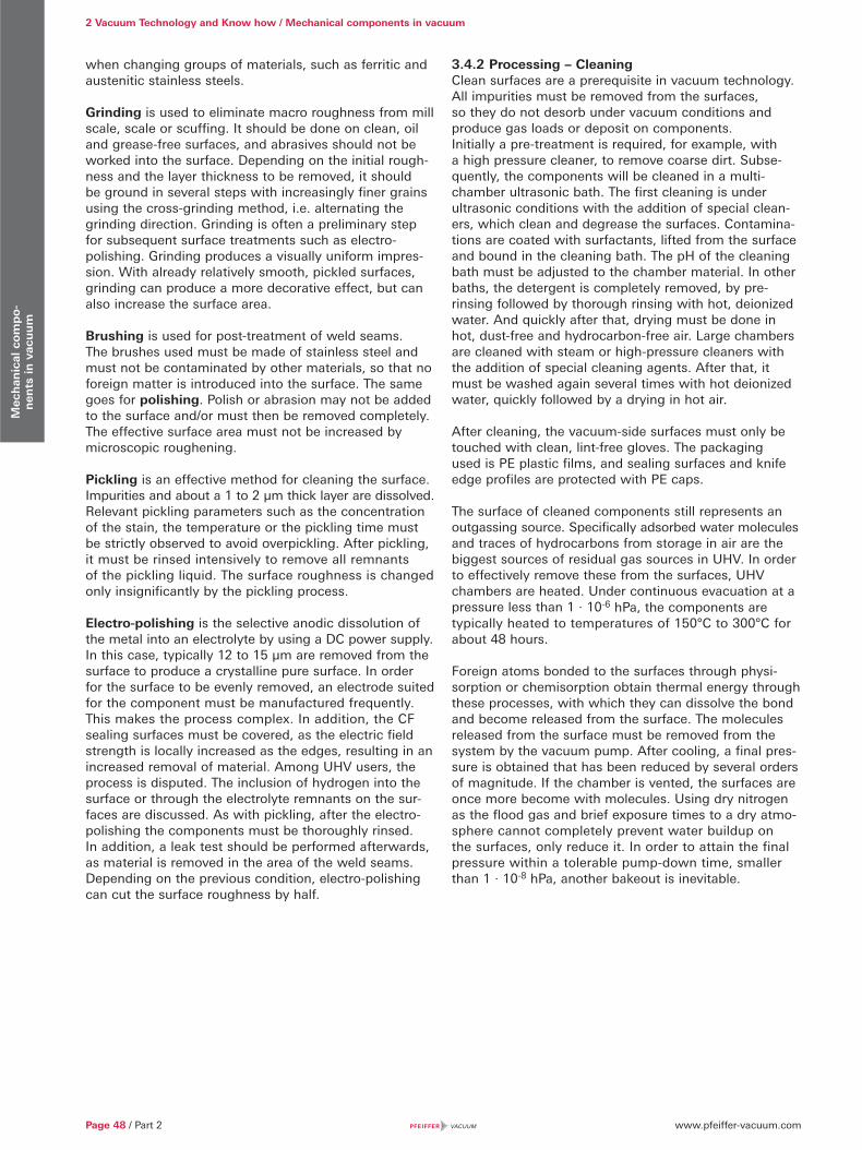
www.pfeiffer-vacuum.comPage 48 / Part 2
2 Vacuum Technology and Know how / Mechanical components in vacuumM
ech
anic
al c
om
po-
nen
ts in
vac
uu
m
when changing groups of materials, such as ferritic and austenitic stainless steels.
Grinding is used to eliminate macro roughness from mill scale, scale or scuffing. It should be done on clean, oil and grease-free surfaces, and abrasives should not be worked into the surface. Depending on the initial rough-ness and the layer thickness to be removed, it should be ground in several steps with increasingly finer grains using the cross-grinding method, i.e. alternating the grinding direction. Grinding is often a preliminary step for subsequent surface treatments such as electro- polishing. Grinding produces a visually uniform impres-sion. With already relatively smooth, pickled surfaces, grinding can produce a more decorative effect, but can also increase the surface area.
Brushing is used for post-treatment of weld seams. The brushes used must be made of stainless steel and must not be contaminated by other materials, so that no foreign matter is introduced into the surface. The same goes for polishing. Polish or abrasion may not be added to the surface and/or must then be removed completely. The effective surface area must not be increased by microscopic roughening.
Pickling is an effective method for cleaning the surface. Impurities and about a 1 to 2 μm thick layer are dissolved. Relevant pickling parameters such as the concentration of the stain, the temperature or the pickling time must be strictly observed to avoid overpickling. After pickling, it must be rinsed intensively to remove all remnants of the pickling liquid. The surface roughness is changed only insignificantly by the pickling process.
Electro-polishing is the selective anodic dissolution of the metal into an electrolyte by using a DC power supply. In this case, typically 12 to 15 μm are removed from the surface to produce a crystalline pure surface. In order for the surface to be evenly removed, an electrode suited for the component must be manufactured frequently. This makes the process complex. In addition, the CF sealing surfaces must be covered, as the electric field strength is locally increased as the edges, resulting in an increased removal of material. Among UHV users, the process is disputed. The inclusion of hydrogen into the surface or through the electrolyte remnants on the sur-faces are discussed. As with pickling, after the electro-polishing the components must be thoroughly rinsed. In addition, a leak test should be performed afterwards, as material is removed in the area of the weld seams. Depending on the previous condition, electro-polishing can cut the surface roughness by half.
3.4.2 Processing – CleaningClean surfaces are a prerequisite in vacuum technology. All impurities must be removed from the surfaces, so they do not desorb under vacuum conditions and produce gas loads or deposit on components. Initially a pre-treatment is required, for example, with a high pressure cleaner, to remove coarse dirt. Subse-quently, the components will be cleaned in a multi-chamber ultrasonic bath. The first cleaning is under ultrasonic conditions with the addition of special clean-ers, which clean and degrease the surfaces. Contamina-tions are coated with surfactants, lifted from the surface and bound in the cleaning bath. The pH of the cleaning bath must be adjusted to the chamber material. In other baths, the detergent is completely removed, by pre- rinsing followed by thorough rinsing with hot, deionized water. And quickly after that, drying must be done in hot, dust-free and hydrocarbon-free air. Large chambers are cleaned with steam or high-pressure cleaners with the addition of special cleaning agents. After that, it must be washed again several times with hot deionized water, quickly followed by a drying in hot air.
After cleaning, the vacuum-side surfaces must only be touched with clean, lint-free gloves. The packaging used is PE plastic films, and sealing surfaces and knife edge profiles are protected with PE caps.
The surface of cleaned components still represents an outgassing source. Specifically adsorbed water molecules and traces of hydrocarbons from storage in air are the biggest sources of residual gas sources in UHV. In order to effectively remove these from the surfaces, UHV chambers are heated. Under continuous evacuation at a pressure less than 1 · 10-6 hPa, the components are typically heated to temperatures of 150°C to 300°C for about 48 hours.
Foreign atoms bonded to the surfaces through physi-sorption or chemisorption obtain thermal energy through these processes, with which they can dissolve the bond and become released from the surface. The molecules released from the surface must be removed from the system by the vacuum pump. After cooling, a final pres-sure is obtained that has been reduced by several orders of magnitude. If the chamber is vented, the surfaces are once more become with molecules. Using dry nitrogen as the flood gas and brief exposure times to a dry atmo-sphere cannot completely prevent water buildup on the surfaces, only reduce it. In order to attain the final pressure within a tolerable pump-down time, smaller than 1 · 10-8 hPa, another bakeout is inevitable.
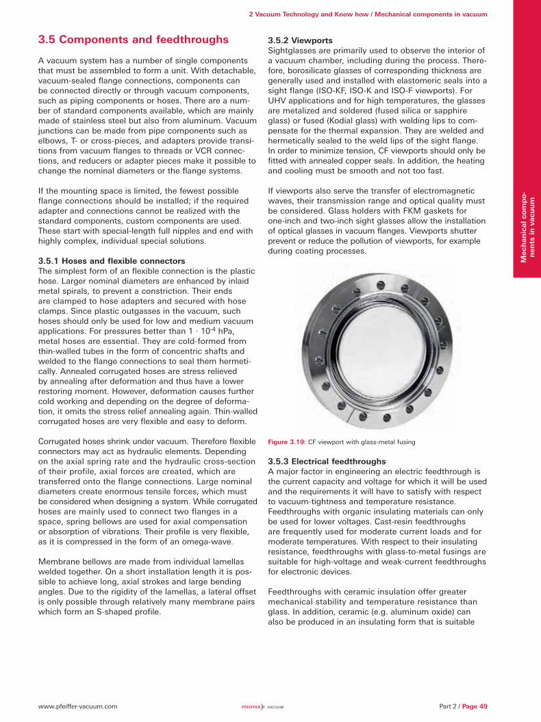
www.pfeiffer-vacuum.com Part 2 / Page 49
2 Vacuum Technology and Know how / Mechanical components in vacuum
Mec
han
ical
com
po-
nen
ts in
vac
uu
m
3.5 Components and feedthroughs
A vacuum system has a number of single components that must be assembled to form a unit. With detachable, vacuum-sealed flange connections, components can be connected directly or through vacuum components, such as piping components or hoses. There are a num-ber of standard components available, which are mainly made of stainless steel but also from aluminum. Vacuum junctions can be made from pipe components such as elbows, T- or cross-pieces, and adapters provide transi-tions from vacuum flanges to threads or VCR connec-tions, and reducers or adapter pieces make it possible to change the nominal diameters or the flange systems.
If the mounting space is limited, the fewest possible flange connections should be installed; if the required adapter and connections cannot be realized with the standard components, custom components are used. These start with special-length full nipples and end with highly complex, individual special solutions.
3.5.1 Hoses and flexible connectorsThe simplest form of an flexible connection is the plastic hose. Larger nominal diameters are enhanced by inlaid metal spirals, to prevent a constriction. Their ends are clamped to hose adapters and secured with hose clamps. Since plastic outgasses in the vacuum, such hoses should only be used for low and medium vacuum applications. For pressures better than 1 · 10-4 hPa, metal hoses are essential. They are cold-formed from thin-walled tubes in the form of concentric shafts and welded to the flange connections to seal them hermeti-cally. Annealed corrugated hoses are stress relieved by annealing after deformation and thus have a lower restoring moment. However, deformation causes further cold working and depending on the degree of deforma-tion, it omits the stress relief annealing again. Thin-walled corrugated hoses are very flexible and easy to deform.
Corrugated hoses shrink under vacuum. Therefore flexible connectors may act as hydraulic elements. Depending on the axial spring rate and the hydraulic cross-section of their profile, axial forces are created, which are transferred onto the flange connections. Large nominal diameters create enormous tensile forces, which must be considered when designing a system. While corrugated hoses are mainly used to connect two flanges in a space, spring bellows are used for axial compensation or absorption of vibrations. Their profile is very flexible, as it is compressed in the form of an omega-wave.
Membrane bellows are made from individual lamellas welded together. On a short installation length it is pos-sible to achieve long, axial strokes and large bending angles. Due to the rigidity of the lamellas, a lateral offset is only possible through relatively many membrane pairs which form an S-shaped profile.
3.5.2 ViewportsSightglasses are primarily used to observe the interior of a vacuum chamber, including during the process. There-fore, borosilicate glasses of corresponding thickness are generally used and installed with elastomeric seals into a sight flange (ISO-KF, ISO-K and ISO-F viewports). For UHV applications and for high temperatures, the glasses are metalized and soldered (fused silica or sapphire glass) or fused (Kodial glass) with welding lips to com-pensate for the thermal expansion. They are welded and hermetically sealed to the weld lips of the sight flange. In order to minimize tension, CF viewports should only be fitted with annealed copper seals. In addition, the heating and cooling must be smooth and not too fast.
If viewports also serve the transfer of electromagnetic waves, their transmission range and optical quality must be considered. Glass holders with FKM gaskets for one-inch and two-inch sight glasses allow the installation of optical glasses in vacuum flanges. Viewports shutter prevent or reduce the pollution of viewports, for example during coating processes.
Figure 3.19: CF viewport with glass-metal fusing
3.5.3 Electrical feedthroughsA major factor in engineering an electric feedthrough is the current capacity and voltage for which it will be used and the requirements it will have to satisfy with respect to vacuum-tightness and temperature resistance. Feedthroughs with organic insulating materials can only be used for lower voltages. Cast-resin feedthroughs are frequently used for moderate current loads and for moderate temperatures. With respect to their insulating resistance, feedthroughs with glass-to-metal fusings are suitable for high-voltage and weak-current feedthroughs for electronic devices.
Feedthroughs with ceramic insulation offer greater mechanical stability and temperature resistance than glass. In addition, ceramic (e.g. aluminum oxide) can also be produced in an insulating form that is suitable
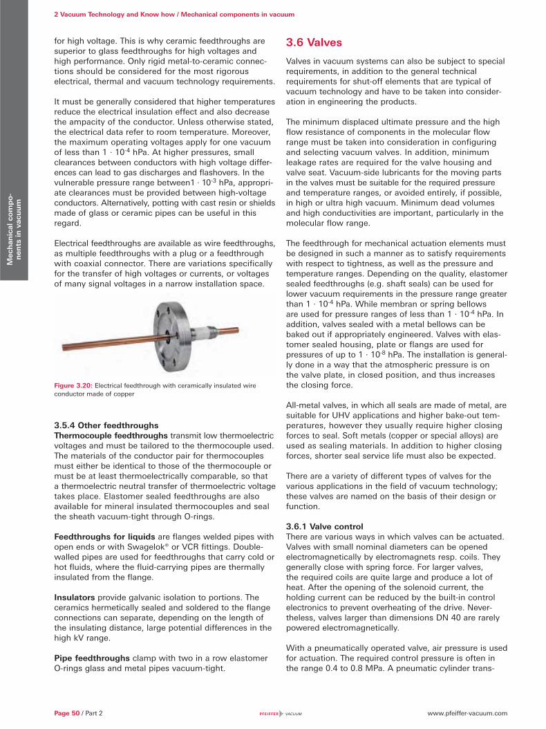
www.pfeiffer-vacuum.comPage 50 / Part 2
2 Vacuum Technology and Know how / Mechanical components in vacuumM
ech
anic
al c
om
po-
nen
ts in
vac
uu
m
for high voltage. This is why ceramic feedthroughs are superior to glass feedthroughs for high voltages and high performance. Only rigid metal-to-ceramic connec-tions should be considered for the most rigorous electrical, thermal and vacuum technology requirements.
It must be generally considered that higher temperatures reduce the electrical insulation effect and also decrease the ampacity of the conductor. Unless otherwise stated, the electrical data refer to room temperature. Moreover, the maximum operating voltages apply for one vacuum of less than 1 · 10-4 hPa. At higher pressures, small clearances between conductors with high voltage differ-ences can lead to gas discharges and flashovers. In the vulnerable pressure range between1 · 10-3 hPa, appropri-ate clearances must be provided between high-voltage conductors. Alternatively, potting with cast resin or shields made of glass or ceramic pipes can be useful in this regard.
Electrical feedthroughs are available as wire feedthroughs, as multiple feedthroughs with a plug or a feedthrough with coaxial connector. There are variations specifically for the transfer of high voltages or currents, or voltages of many signal voltages in a narrow installation space.
Figure 3.20: Electrical feedthrough with ceramically insulated wire conductor made of copper
3.5.4 Other feedthroughs Thermocouple feedthroughs transmit low thermoelectric voltages and must be tailored to the thermocouple used. The materials of the conductor pair for thermocouples must either be identical to those of the thermocouple or must be at least thermoelectrically comparable, so that a thermoelectric neutral transfer of thermoelectric voltage takes place. Elastomer sealed feedthroughs are also available for mineral insulated thermocouples and seal the sheath vacuum-tight through O-rings.
Feedthroughs for liquids are flanges welded pipes with open ends or with Swagelok® or VCR fittings. Double-walled pipes are used for feedthroughs that carry cold or hot fluids, where the fluid-carrying pipes are thermally insulated from the flange.
Insulators provide galvanic isolation to portions. The ceramics hermetically sealed and soldered to the flange connections can separate, depending on the length of the insulating distance, large potential differences in the high kV range.
Pipe feedthroughs clamp with two in a row elastomer O-rings glass and metal pipes vacuum-tight.
3.6 Valves
Valves in vacuum systems can also be subject to special requirements, in addition to the general technical requirements for shut-off elements that are typical of vacuum technology and have to be taken into consider-ation in engineering the products.
The minimum displaced ultimate pressure and the high flow resistance of components in the molecular flow range must be taken into consideration in configuring and selecting vacuum valves. In addition, minimum leakage rates are required for the valve housing and valve seat. Vacuum-side lubricants for the moving parts in the valves must be suitable for the required pressure and temperature ranges, or avoided entirely, if possible, in high or ultra high vacuum. Minimum dead volumes and high conductivities are important, particularly in the molecular flow range.
The feedthrough for mechanical actuation elements must be designed in such a manner as to satisfy requirements with respect to tightness, as well as the pressure and temperature ranges. Depending on the quality, elastomer sealed feedthroughs (e.g. shaft seals) can be used for lower vacuum requirements in the pressure range greater than 1 · 10-4 hPa. While membran or spring bellows are used for pressure ranges of less than 1 · 10-4 hPa. In addition, valves sealed with a metal bellows can be baked out if appropriately engineered. Valves with elas-tomer sealed housing, plate or flangs are used for pressures of up to 1 · 10-8 hPa. The installation is general-ly done in a way that the atmospheric pressure is on the valve plate, in closed position, and thus increases the closing force.
All-metal valves, in which all seals are made of metal, are suitable for UHV applications and higher bake-out tem-peratures, however they usually require higher closing forces to seal. Soft metals (copper or special alloys) are used as sealing materials. In addition to higher closing forces, shorter seal service life must also be expected.
There are a variety of different types of valves for the various applications in the field of vacuum technology; these valves are named on the basis of their design or function.
3.6.1 Valve controlThere are various ways in which valves can be actuated. Valves with small nominal diameters can be opened electromagnetically by electromagnets resp. coils. They generally close with spring force. For larger valves, the required coils are quite large and produce a lot of heat. After the opening of the solenoid current, the holding current can be reduced by the built-in control electronics to prevent overheating of the drive. Never- theless, valves larger than dimensions DN 40 are rarely powered electromagnetically.
With a pneumatically operated valve, air pressure is used for actuation. The required control pressure is often in the range 0.4 to 0.8 MPa. A pneumatic cylinder trans-
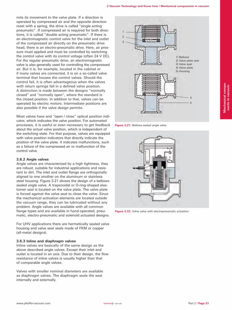
www.pfeiffer-vacuum.com Part 2 / Page 51
2 Vacuum Technology and Know how / Mechanical components in vacuum
Mec
han
ical
com
po-
nen
ts in
vac
uu
m
mits its movement to the valve plate. If a direction is operated by compressed air and the opposite direction reset with a spring, the drive is called “single acting pneumatic”. If compressed air is required for both direc-tions, it is called “double acting pneumatic”. If there is an electromagnetic control valve for the inlet and outlet of the compressed air directly on the pneumatic drive head, there is an electro-pneumatic drive. Here, air pres-sure must applied and must be controlled by switching the control valve with its control voltage (often 24 V DC). For the regular pneumatic drive, an electromagnetic valve is also generally used for controlling the compressed air. But it is, for example, located in the cabinet or if many valves are connected, it is on a so-called valve terminal that houses the control valves. Should the control fail, it is often advantageous when the valves with return springs fall in a defined valve position. A distinction is made between the designs “normally closed” and “normally open“, where the standard is the closed position. In addition to that, valves can be operated by electric motors. Intermediate positions are also possible if the valve design permits.
Most valves have and “open / close” optical position indi-cator, which indicates the valve position. For automated processes, it is useful or even necessary to get feedback about the actual valve position, which is independent of the switching state. For that purpose, valves are equipped with valve position indicators that directly indicate the position of the valve plate. It indicates malfunctions, such as a failure of the compressed air or malfunction of the control valve.
3.6.2 Angle valvesAngle valves are characterized by a high tightness, they are robust, suitable for industrial applications and resis-tant to dirt. The inlet and outlet flange are orthogonally aligned to one another on the aluminum or stainless steel housing. Figure 3.21 shows the design of a bellows-sealed angle valve. A trapezoidal or O-ring-shaped elas-tomer seal is located on the valve plate. The valve plate is forced against the valve seat to close the valve. Since the mechanical activation elements are located outside the vacuum range, they can be lubricated without any problem. Angle valves are available with all common flange types and are available in hand-operated, pneu-matic, electro-pneumatic and solenoid actuated designs.
For UHV applications there are hermetically sealed valve housing and valve seat seals made of FKM or copper (all-metal designs).
3.6.3 Inline and diaphragm valvesInline valves are basically of the same design as the above described angle valves. Except their inlet and outlet is located in an axis. Due to their design, the flow resistance of inline valves is usually higher than that of comparable angle valves.
Valves with smaller nominal diameters are available as diaphragm valves. The diaphragm seals the seat internally and externally.
Figure 3.21: Bellows-sealed angle valve
Figure 3.22: Inline valve with electropneumatic actuation
1) Bellows2) Valve plate seal3) Valve seat4) Valve plate5) Housing
1
2
3
4
5
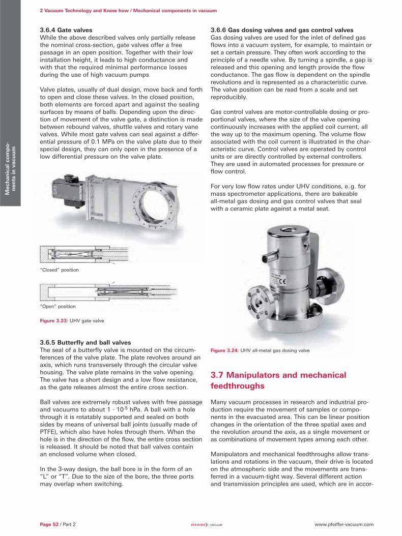
www.pfeiffer-vacuum.comPage 52 / Part 2
2 Vacuum Technology and Know how / Mechanical components in vacuumM
ech
anic
al c
om
po-
nen
ts in
vac
uu
m
3.6.4 Gate valvesWhile the above described valves only partially release the nominal cross-section, gate valves offer a free passage in an open position. Together with their low installation height, it leads to high conductance and with that the required minimal performance losses during the use of high vacuum pumps
Valve plates, usually of dual design, move back and forth to open and close these valves. In the closed position, both elements are forced apart and against the sealing surfaces by means of balls. Depending upon the direc-tion of movement of the valve gate, a distinction is made between rebound valves, shuttle valves and rotary vane valves. While most gate valves can seal against a differ-ential pressure of 0.1 MPa on the valve plate due to their special design, they can only open in the presence of a low differential pressure on the valve plate.
Figure 3.23: UHV gate valve
3.6.5 Butterfly and ball valves The seal of a butterfly valve is mounted on the circum-ferences of the valve plate. The plate revolves around an axis, which runs transversely through the circular valve housing. The valve plate remains in the valve opening. The valve has a short design and a low flow resistance, as the gate releases almost the entire cross section.
Ball valves are extremely robust valves with free passage and vacuums to about 1 · 10-5 hPa. A ball with a hole through it is rotatably supported and sealed on both sides by means of universal ball joints (usually made of PTFE), which also have holes through them. When the hole is in the direction of the flow, the entire cross section is released. It should be noted that ball valves contain an enclosed volume when closed.
In the 3-way design, the ball bore is in the form of an “L” or “T”. Due to the size of the bore, the three ports may overlap when switching.
3.6.6 Gas dosing valves and gas control valvesGas dosing valves are used for the inlet of defined gasflows into a vacuum system, for example, to maintain or set a certain pressure. They often work according to the principle of a needle valve. By turning a spindle, a gap is released and this opening and length provide the flow conductance. The gas flow is dependent on the spindle revolutions and is represented as a characteristic curve. The valve position can be read from a scale and set reproducibly.
Gas control valves are motor-controllable dosing or pro-portional valves, where the size of the valve opening continuously increases with the applied coil current, all the way up to the maximum opening. The volume flow associated with the coil current is illustrated in the char-acteristic curve. Control valves are operated by control units or are directly controlled by external controllers. They are used in automated processes for pressure or flow control.
For very low flow rates under UHV conditions, e. g. for mass spectrometer applications, there are bakeable all-metal gas dosing and gas control valves that seal with a ceramic plate against a metal seat.
Figure 3.24: UHV all-metal gas dosing valve
3.7 Manipulators and mechanical feedthroughs
Many vacuum processes in research and industrial pro-duction require the movement of samples or compo-nents in the evacuated area. This can be linear position changes in the orientation of the three spatial axes and the revolution around the axis, as a single movement or as combinations of movement types among each other.
Manipulators and mechanical feedthroughs allow trans-lations and rotations in the vacuum, their drive is located on the atmospheric side and the movements are trans-ferred in a vacuum-tight way. Several different action and transmission principles are used, which are in accor-
“Closed” position
“Open” position

www.pfeiffer-vacuum.com Part 2 / Page 53
2 Vacuum Technology and Know how / Mechanical components in vacuum
Mec
han
ical
com
po-
nen
ts in
vac
uu
m
dance with the respective and vacuum and application conditions. Metalic membrane and spring bellows, special elastomer seals, magnetically coupled systems or differentially pumped seals can be used as sealing elements.
The designs with two open flange connections and an open passage are called manipulators, and components that have an actuator installed in a vacuum-tight flange are called mechanical feedthroughs. The latter are characterized by a compact design. Manipulators can be combined and extended among each other. In addition, mechanical feedthroughs can be attached to them, so that diverse types of movements transfer into the vacuum and with that provide solutions for various motion tasks. Additionally, other feedthroughs can be attached to the inlet flange, for example, for electricity or fluids and these can be guided by the manipulator directly to the application.
Especially with larger nominal diameters, the flanges of manipulators are under considerable forces due to the atmospheric pressure. So that the flanges are stable under vacuum, great emphasis must be placed on their inherent rigidity during the design of manipulators. The particular design challenge is to bring the highly precise transmission of movements in accordance with the external load and other loads by built-in components. The built-in components must be able to be baked out, in order to ensure the use even in the UHV range.
3.7.1 Operating principlesWhen selecting a suitable manipulator or a mechanical implementation, the user should know the underlying principle, to be able to assess the technical parameters regarding the suitability for its tasks.
3.7.1.1 Translation sealed by diaphragm bellowsMembrane bellows are made from individual lamellas welded together. With a small spring rate, the axial expansion is highly flexible. Bellows ensure a hermetically sealed metal enclosure and are suitable for the highest UHV requirements.
The selection and design of the bellows is in accordance with the required movement task, taking into account the operating conditions: Service life (number of move-ment cycles), operating temperature, bakeout tempera-ture, differential pressures. The lifetime can be up to 0.5 million cycles with membranes made from the material 316L and up to 10 million movement cycles for the more elastic but magnetizable material 350AM.
Membrane bellows within the specified number of cycles are maintenance free. After they reach the calculated motion cycles they need to be replaced. They are not suitable for environments with dust and dirt.
Membrane bellows are used in the Z-axis, XY-axis and XYZ-axis precision manipulators, and port aligners and bellows sealed rotary feedthroughs.
When baking out units with diaphragm bellows, it is important to ensure an even heating. Heater bands on diaphragm bellows should be avoided. They lead to a strong local heating, as the diaphragm bellows have a low mass and a small area for the heat conduction. Temperature controlled heating sleeves are the better, though more elaborate alternative.
3.7.1.2 Bellows-sealed rotationThe so-called cattail or wobble principle allows the trans-mission of a rotational movement with bellows, i. e. rotary motion with a hermetic separation between vacuum and atmosphere. Figure 3.25 shows the design of such a feedthrough. The angled drive shaft (1), whose end is supported in a crank pin (3), rotates the drive shaft (4) in the vacuum. The hermetic seal consists of a non-rotating bellows seal (2) that performs a wobbling movement. Driven and drive shaft are supported by stainless steel ball bearings, which are coated with a vacuum-suitable dry-lubrication.
The dry lubrication increases not only the service life and possible maximum speed, it also prevents that the balls get stuck during the bake out at high temperatures. In addition to dry lubrication, hybrid bearings with ceramic balls can also be used for UHV applications. Their high price justifies a use only for the highest standards. Alter-natively, for high vacuum applications that are resistant to small amounts of hydrocarbons, bearings can be lubricated with vacuum-suitable grease.
Figure 3.25: Bellows-sealed UHV rotary feedthrough (cattail principle)
1) Drive shaft2) Spring bellows3) Crank pin
4) Driven shaft5) Ball bearings6) CF flange
1
2
536
45
5Vacuum
Atmosphere
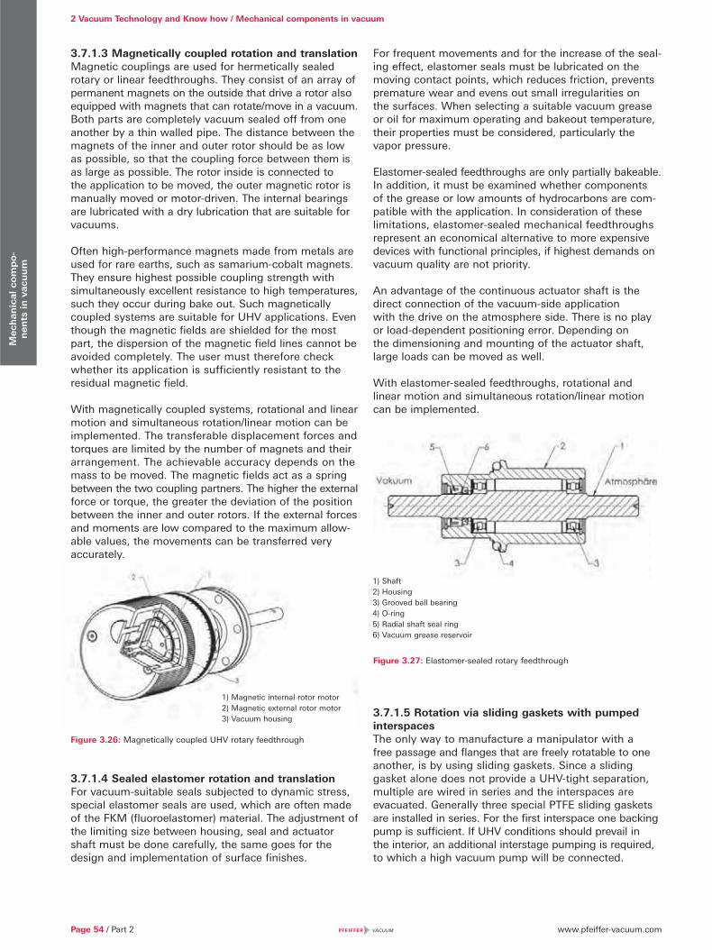
www.pfeiffer-vacuum.comPage 54 / Part 2
2 Vacuum Technology and Know how / Mechanical components in vacuumM
ech
anic
al c
om
po-
nen
ts in
vac
uu
m
3.7.1.3 Magnetically coupled rotation and translationMagnetic couplings are used for hermetically sealed rotary or linear feedthroughs. They consist of an array of permanent magnets on the outside that drive a rotor also equipped with magnets that can rotate/move in a vacuum. Both parts are completely vacuum sealed off from one another by a thin walled pipe. The distance between the magnets of the inner and outer rotor should be as low as possible, so that the coupling force between them is as large as possible. The rotor inside is connected to the application to be moved, the outer magnetic rotor is manually moved or motor-driven. The internal bearings are lubricated with a dry lubrication that are suitable for vacuums.
Often high-performance magnets made from metals are used for rare earths, such as samarium-cobalt magnets. They ensure highest possible coupling strength with simultaneously excellent resistance to high temperatures, such they occur during bake out. Such magnetically coupled systems are suitable for UHV applications. Even though the magnetic fields are shielded for the most part, the dispersion of the magnetic field lines cannot be avoided completely. The user must therefore check whether its application is sufficiently resistant to the residual magnetic field.
With magnetically coupled systems, rotational and linear motion and simultaneous rotation/linear motion can be implemented. The transferable displacement forces and torques are limited by the number of magnets and their arrangement. The achievable accuracy depends on the mass to be moved. The magnetic fields act as a spring between the two coupling partners. The higher the external force or torque, the greater the deviation of the position between the inner and outer rotors. If the external forces and moments are low compared to the maximum allow-able values, the movements can be transferred very accurately.
Figure 3.26: Magnetically coupled UHV rotary feedthrough
3.7.1.4 Sealed elastomer rotation and translationFor vacuum-suitable seals subjected to dynamic stress, special elastomer seals are used, which are often made of the FKM (fluoroelastomer) material. The adjustment of the limiting size between housing, seal and actuator shaft must be done carefully, the same goes for the design and implementation of surface finishes.
For frequent movements and for the increase of the seal-ing effect, elastomer seals must be lubricated on the moving contact points, which reduces friction, prevents premature wear and evens out small irregularities on the surfaces. When selecting a suitable vacuum grease or oil for maximum operating and bakeout temperature, their properties must be considered, particularly the vapor pressure.
Elastomer-sealed feedthroughs are only partially bakeable. In addition, it must be examined whether components of the grease or low amounts of hydrocarbons are com-patible with the application. In consideration of these limitations, elastomer-sealed mechanical feedthroughs represent an economical alternative to more expensive devices with functional principles, if highest demands on vacuum quality are not priority.
An advantage of the continuous actuator shaft is the direct connection of the vacuum-side application with the drive on the atmosphere side. There is no play or load-dependent positioning error. Depending on the dimensioning and mounting of the actuator shaft, large loads can be moved as well.
With elastomer-sealed feedthroughs, rotational and linear motion and simultaneous rotation/linear motion can be implemented.
Figure 3.27: Elastomer-sealed rotary feedthrough
3.7.1.5 Rotation via sliding gaskets with pumped interspacesThe only way to manufacture a manipulator with a free passage and flanges that are freely rotatable to one another, is by using sliding gaskets. Since a sliding gasket alone does not provide a UHV-tight separation, multiple are wired in series and the interspaces are evacuated. Generally three special PTFE sliding gaskets are installed in series. For the first interspace one backing pump is sufficient. If UHV conditions should prevail in the interior, an additional interstage pumping is required, to which a high vacuum pump will be connected.
1) Shaft2) Housing3) Grooved ball bearing4) O-ring5) Radial shaft seal ring6) Vacuum grease reservoir
1) Magnetic internal rotor motor2) Magnetic external rotor motor3) Vacuum housing
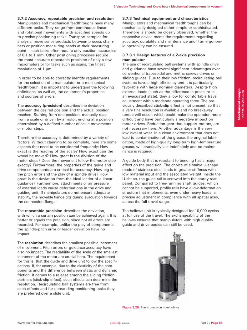
www.pfeiffer-vacuum.com Part 2 / Page 55
2 Vacuum Technology and Know how / Mechanical components in vacuum
Mec
han
ical
com
po-
nen
ts in
vac
uu
m
3.7.2 Accuracy, repeatable precision and resolutionManipulators and mechanical feedthroughs have many different tasks. They range from continuous linear and rotational movements with specified speeds up to precise positioning tasks. Transport samples for analysis, move series products between process cham-bers or position measuring heads at their measuring point – such tasks often require only position accuracies of 0.1 to 1 mm. Other positioning processes require the most accurate repeatable precision of only a few micrometers or for tasks such as scans, the finest resolutions of 1 μm.
In order to be able to correctly identify requirements for the selection of a manipulator or a mechanical feedthrough, it is important to understand the following definitions, as well as, the equipment's properties and sources of errors.
The accuracy (precision) describes the deviation between the desired position and the actual position reached. Starting from one position, manually read from a scale or driven by a motor, ending at a position determined by a defined number of scale movements or motor steps.
Therefore the accuracy is determined by a variety of factors. Without claiming to be complete, here are some aspects that need to be considered frequently: How exact is the reading of the scale? How exact can the wheel be moved? How great is the division of the motor steps? Does the movement follow the motor step exactly? Furthermore, the properties of the guide and drive components are critical for accuracy: How big is the pitch error and the play of a spindle drive? How great is the deviation from the ideal leader of a linear guidance? Furthermore, attachments or air pressure of external loads cause deformations in the drive and guiding unit. If manipulators do not ensure adequate stability, the movable flange tilts during evacuation towards the connection flange.
The repeatable precision describes the deviation, with which a certain position can be achieved again. It is better or equals the precision, since not all errors are recorded. For example, unlike the play of components, the spindle-pitch error or leader deviation have no impact.
The resolution describes the smallest possible increment of movement. Pitch errors or guidance accuracy have also no impact. The readability of the scale or the smallest increment of the motor are crucial here. The requirement for this is, that the guide and drive unit follow the specifi-cations. If, for example, due to the elasticity of the com-ponents and the difference between static and dynamic friction, it comes to a release among the sliding friction partners (stick-slip effect), such effects can determine the resolution. Recirculating ball systems are free from such effects and for demanding positioning tasks they are preferred over a slide unit.
3.7.3 Technical equipment and characteristicsManipulators and mechanical feedthroughs can be mechanically designed either simple or sophisticated. Therefore is should be closely observed, whether the respective device meets the requirements regarding accuracy, durability and maintenance and if an ergonom-ic operability can be ensured.
3.7.3.1 Design features of a Z-axis precision manipulatorThe use of recirculating ball systems with spindle drive and guidance have several significant advantages over conventional trapezoidal and metric screws drives or sliding guides. Due to their low friction, recirculating ball systems have a high efficiency and it is particularly favorable with large nominal diameters. Despite high external loads (such as the difference in pressure in an evacuated state), they allow for comfortable travel adjustment with a moderate operating force. The pre-viously described stick-slip effect is not present, so that a very fine resolution is available and no breakaway torque will occur, which could make the operation more difficult and have particularly a negative impact on motor drives. Reduction gear that support motors, are not necessary here. Another advantage is the very low level of wear. In a clean environment that does not lead to contamination of the grease, the original lubri-cation, made of high-quality long-term high-temperature grease, will practically last indefinitely and no mainte-nance is required.
A guide body that is resistant to bending has a major effect on the precision. The choice of a stable U-shape made of stainless steel leads to greater stiffness with low material input and the associated weight. Inside the U-shape, the guide rail is screwed into the sturdy rear panel. Compared to free-running shaft guides, which cannot be supported, profile rails have a low-deformation structure that implements, even under heavy loads, a precise adjustment in compliance with all spatial axes, across the full travel range.
The bellows unit is typically designed for 10,000 cycles at full use of the travel. The exchangeability of the bellows ensures that manipulators with high quality guide and drive bodies can still be used.
Figure 3.28: Z-axis precision manipulator
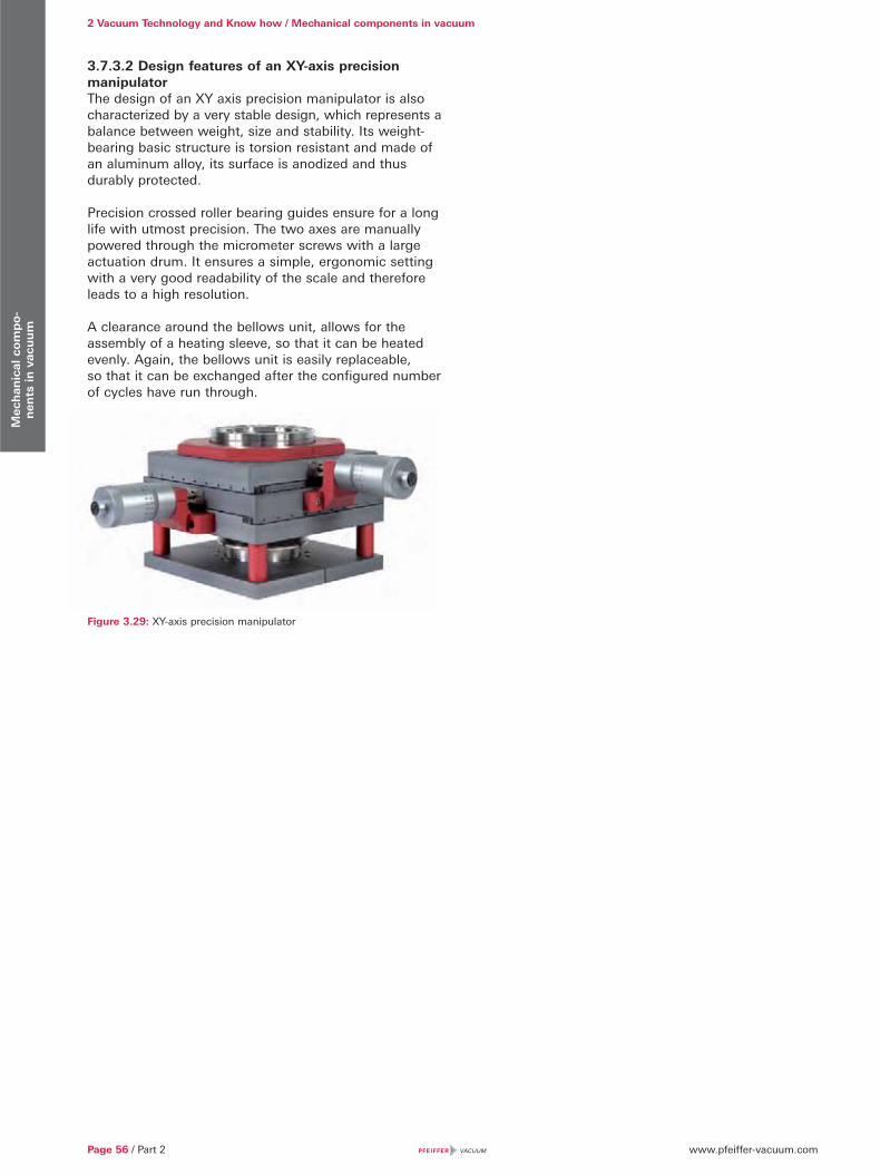
www.pfeiffer-vacuum.comPage 56 / Part 2
2 Vacuum Technology and Know how / Mechanical components in vacuumM
ech
anic
al c
om
po-
nen
ts in
vac
uu
m
3.7.3.2 Design features of an XY-axis precision manipulatorThe design of an XY axis precision manipulator is also characterized by a very stable design, which represents a balance between weight, size and stability. Its weight-bearing basic structure is torsion resistant and made of an aluminum alloy, its surface is anodized and thus durably protected.
Precision crossed roller bearing guides ensure for a long life with utmost precision. The two axes are manually powered through the micrometer screws with a large actuation drum. It ensures a simple, ergonomic setting with a very good readability of the scale and therefore leads to a high resolution.
A clearance around the bellows unit, allows for the assembly of a heating sleeve, so that it can be heated evenly. Again, the bellows unit is easily replaceable, so that it can be exchanged after the configured number of cycles have run through.
Figure 3.29: XY-axis precision manipulator
www.pfeiffer-vacuum.com Part 2 / Page 57
2 Vacuum Technology and Know how / Mechanical components in vacuum
Mec
han
ical
com
po-
nen
ts in
vac
uu
m

www.pfeiffer-vacuum.comPage 58 / Part 2
Vac
uu
m g
ener
atio
n
4 Vacuum generation
4.1 Vacuum pumps – working principles and properties
4.1.1 Classification of vacuum pumpsVacuum pumps are categorized as gas transfer pumps and gas binding or capture pumps. While gas-displace-ment vacuum pumps can be used without limitation, gas-binding vacuum pumps have a limited gas absorption capacity and must be regenerated at certain process-dependent intervals.
Gas-displacement pumps, which are also referred to as gas transfer pumps, are classified either as positive
displacement pumps or kinetic vacuum pumps. Positive displacement pumps displace gas from sealed areas to the atmosphere or to a downstream pump stage. Kinetic pumps displace gas by accelerating it in the pumping direction, either via a mechanical drive system or through a directed vapor stream that is condensed at the end of the pumping section. Gas-binding vacuum pumps either bind the gas to an especially active substrate through gettering or condense the gas at a suitable temperature. Chemisorption is performed technically by a pump type known as getter pumps which constantly generate pure getter surfaces through vaporization and/or sublimation or sputtering. If the gas particles to be bound are ionized in an ion getter pump before interacting with a getter
Figure 4.1: Overview of vacuum pumps
Gas-DisplacementVacuum Pumps
KineticVacuum Pumps
Gas TransferVacuum Pumps
Gas-BindingVacuum Pumps
Vacuum Pumps(Operating Principle)
Liquid JetPump
Gas Ring (SideChannel) Pump
Propellant JetPump
Getter Pumps
Rotary VanePump
Turbo-Pumps
Liquid JetPump
Massive GetterPump
Multi-CellPump
Rotary PistonPump
External VanePump
AxialPump
RadialPump
MolecularPump
TurbomolecularPump
Gas JetPump
Steam JetPump
DiffusionPump
Diffusion EjectorPump
Sublimation Vaporization
Pump
Ion GetterPump
Cryo Pump
Condenser
MechanicalKineticPumps
PropellantPumps
Ion TransferPump
AdsorptionPumps
DiaphragmPump
PistonPump
Scroll Pump
RootsPump
ScrewPump
Claw-Type Piston Pump
Double-RotorDisplacement
Pumps
OscillationDisplacement
Pumps
Single-RotorDisplacement
Pumps
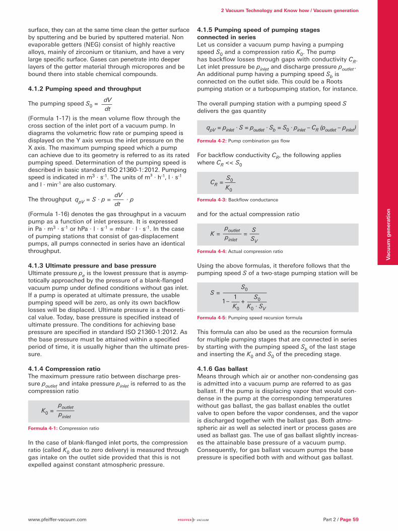
www.pfeiffer-vacuum.com
2 Vacuum Technology and Know how / Vacuum generation
Part 2 / Page 59
Vac
uu
m g
ener
atio
n
surface, they can at the same time clean the getter surface by sputtering and be buried by sputtered material. Non evaporable getters (NEG) consist of highly reactive alloys, mainly of zirconium or titanium, and have a very large specific surface. Gases can penetrate into deeper layers of the getter material through micropores and be bound there into stable chemical compounds.
4.1.2 Pumping speed and throughput
The pumping speed S0 =
(Formula 1-17) is the mean volume flow through the cross section of the inlet port of a vacuum pump. In diagrams the volumetric flow rate or pumping speed is displayed on the Y axis versus the inlet pressure on the X axis. The maximum pumping speed which a pump can achieve due to its geometry is referred to as its rated pumping speed. Determination of the pumping speed is described in basic standard ISO 21360-1: 2012. Pumping speed is indicated in m3 · s-1. The units of m³ · h-1, l · s-1 and l · min-1 are also customary.
The throughput
(Formula 1-16) denotes the gas throughput in a vacuum pump as a function of inlet pressure. It is expressed in Pa · m3 · s-1 or hPa · l · s-1 = mbar · l · s-1. In the case of pumping stations that consist of gas-displacement pumps, all pumps connected in series have an identical throughput.
4.1.3 Ultimate pressure and base pressureUltimate pressure pe is the lowest pressure that is asymp-totically approached by the pressure of a blank-flanged vacuum pump under defined conditions without gas inlet. If a pump is operated at ultimate pressure, the usable pumping speed will be zero, as only its own backflow losses will be displaced. Ultimate pressure is a theoreti-cal value. Today, base pressure is specified instead of ultimate pressure. The conditions for achieving base pressure are specified in standard ISO 21360-1:2012. As the base pressure must be attained within a specified period of time, it is usually higher than the ultimate pres-sure.
4.1.4 Compression ratioThe maximum pressure ratio between discharge pres-sure poutlet and intake pressure pinlet is referred to as the compression ratio
Formula 4-1: Compression ratio
In the case of blank-flanged inlet ports, the compression ratio (called K0 due to zero delivery) is measured through gas intake on the outlet side provided that this is not expelled against constant atmospheric pressure.
4.1.5 Pumping speed of pumping stages connected in seriesLet us consider a vacuum pump having a pumping speed S0 and a compression ratio K0. The pump has backflow losses through gaps with conductivity CR. Let inlet pressure be pinlet and discharge pressure poutlet . An additional pump having a pumping speed Sb is connected on the outlet side. This could be a Roots pumping station or a turbopumping station, for instance.
The overall pumping station with a pumping speed S delivers the gas quantity
Formula 4-2: Pump combination gas flow
For backflow conductivity CR, the following applies where CR << S0
Formula 4-3: Backflow conductance
and for the actual compression ratio
Formula 4-4: Actual compression ratio
Using the above formulas, it therefore follows that the pumping speed S of a two-stage pumping station will be
Formula 4-5: Pumping speed recursion formula
This formula can also be used as the recursion formula for multiple pumping stages that are connected in series by starting with the pumping speed Sb of the last stage and inserting the K0 and S0 of the preceding stage.
4.1.6 Gas ballastMeans through which air or another non-condensing gas is admitted into a vacuum pump are referred to as gas ballast. If the pump is displacing vapor that would con-dense in the pump at the corresponding temperatures without gas ballast, the gas ballast enables the outlet valve to open before the vapor condenses, and the vapor is discharged together with the ballast gas. Both atmo-spheric air as well as selected inert or process gases are used as ballast gas. The use of gas ballast slightly increas-es the attainable base pressure of a vacuum pump. Consequently, for gas ballast vacuum pumps the base pressure is specified both with and without gas ballast.
qpV = pinlet · S = poutlet · Sb = S0 · pinlet – CR (poutlet – pinlet )
S0
K0
CR =
dV
dt
qpV = S · p = · pdV
dt
poutlet
pinletK0 =
poutlet
pinletK = =
S
SV
S0
1 – + 1 S0
K0 K0 · SV
S =

www.pfeiffer-vacuum.comPage 60 / Part 2
2 Vacuum Technology and Know how / Vacuum generationV
acu
um
gen
erat
ion
4.1.7 Water vapor tolerance / water vapor capacity Water vapor tolerance pw is the maximum water vapor pressure with which a vacuum pump can continuously intake and displace pure water vapor under normal ambient conditions (20 °C, p0 = 1,013 hPa). It can be calculated from the pumping speed, gas ballast flow, relative humidity and saturation vapor pressure at a given pump temperature.
Formula 4-6: Water vapor tolerance
pW Water vapor toleranceqpV, Ballast Gas ballast flowS Pumping speed of pumppS Saturation vapor pressure of water vapor at exhaust gas temperaturepa Partial pressure of water vapor in the airp0 Atmospheric pressure� Correction factor, dimensionless
The correction factor takes into account the fact that a higher pressure than atmospheric pressure is required to open the outlet valve. In our example � can be assumed as 1.1.
The water vapor tolerance has the dimension of a pressure and is expressed in hPa.
DIN 28426 describes the use of an indirect process to determine water vapor tolerance. The water vapor tolerance increases as the exhaust temperature of the pump rises and gas ballast flow qpV,Ballast increases. It decreases at higher ambient pressure.
Without gas ballast, a vacuum pump having an outlet temperature of less than 100°C would not be capable of displacing even small amounts of pure water vapor. If water vapor is nevertheless pumped without gas ballast, the condensate will dissolve in the pump oil. As a result, the base pressure will rise and the condensate could cause corrosion damage.
The water vapor capacity is the maximum volume of water that a vacuum pump can continuously intake and displace in the form of water vapor under the ambient conditions of 20 °C and 1,013 hPa.
Formula 4-7: Water vapor capacity
qm,water Water vapor capacityM Molar mass of waterR General gas constantT Absolute temperature
The water vapor capacity is expressed in g · h-1. It is therefore a water vapor mass flow rate. The symbol cW (water vapor capacity) is commonly used to express this in formulas.
4.1.8 Sealing gasWhen pumping corrosive process gas, there is a risk that the gas might attack parts of the pump. To counter this danger, sensitive parts must be protected by a continuous flow of inert gas. Pumps are therefore fitted with a special gas inlet system through which gas flows into the pumping system at defined locations. In turbo-molecular pumps, it is principally the bearings and the motor compartment which require protection. The intake of sealing gas in the motor compartment protects against chemical reactions by aggressive gases with corosion-sensitive components of the lubricant or the bearings as well as preventing dust and particles entering the lubricant reservoir and mixing with the lubricant. The use of sealing gas to protect the motor and prevent particles from entering and causing contact betweenthe shaft and the emergency bearings, for instance, is also recommended for lubricant-free turbopumps.
In addition to sealing gas for the bearings, process-capa-ble dry backing pumps also have purge gas injected into individual pumping stages of the process pump. The process-dependent purge gas flow is adjusted using pressure regulators upstream of the calibrated nozzles or flow regulators (mass flow controllers, or MFC) and monitored by pressure sensors and switches.
4.2 Rotary vane vacuum pumps4.2.1 Design / Operating principleA rotary vane vacuum pump is an oil-sealed rotary dis-placement pump. The pumping system consists of a housing (1), an eccentrically installed rotor (2), vanes (3) that move radially under centrifugal and resilient forces and the inlet and outlet (4). The inlet valve, if available, is designed as a vacuum safety valve that is always open during operation. The working chamber (5) is located inside the housing and is restricted by the stator, rotor and the vanes. The eccentrically installed rotor and vanes divide the working chamber into two separate compartments with variable volumes. As the rotor turns, gas flows into the enlarging suction chamber until it is sealed off by the second vane. The enclosed gas is then compressed until the outlet valve opens against atmospheric pressure. The outlet valve is oil-sealed.
qpV, ballast · (pS – pa )
S · (� · p0 – pS)pW =
qm, water = pW · S · M · (RT) -1
1) Housing
2) Rotor
3) Vane
4) Inlet / Outlet
5) Working chamber
6) Outlet valve
6
1
2
35
4
Figure 4.2: Operating principle of a rotary vane pump
www.pfeiffer-vacuum.com
2 Vacuum Technology and Know how / Vacuum generation
Part 2 / Page 61
Vac
uu
m g
ener
atio
n
When the valve is open, a small amount of oil enters the suction chamber and not only lubricates it but also seals the vanes against the housing (stator).
In the case of gas ballast operation, a hole to the outside is opened, which empties into the sealed suction cham-ber on the front side. As a result, the pressure needed to open the outlet valve is attained at relatively low com-pression during the compression pumping phase. This allows a displaced gas/vapor mixture to be expelled before the vapor starts to condense. The final pressure reached during operation with gas ballast is higher than in operation without gas ballast.
Operating fluid, oilPump oil, which is also referred to as operating fluid, has multiple tasks to perform in a rotary vane pump. It lubri-cates all moving parts, fills both the dead volume under the outlet valve as well as the narrow gap between the inlet and outlet. It compresses the gap between the vanes and the working chamber and additionally ensures an optimal temperature balance through heat transfer.
Multi-stage pumpsRotary vane vacuum pumps are built in single- and two-stage versions. Two-stage pumps achieve lower ultimate pressures than single-stage pumps. Moreover, the effects of the gas ballast on the ultimate pressure are lower, as the ballast gas is only admitted at the high pressure stage.
Vacuum safety valveDepending upon the type of pump in question, rotary vane vacuum pumps may be equipped with a vacuum safety valve. The vacuum safety valve isolates the pump from the vacuum chamber in the event of intentional or unintentional standstill, and uses the displaced gas to vent the pumping system in order to prevent oil from rising into the vacuum chamber. After switching on the pump, it opens after a delay once the pressure in the pump has reached the approximate pressure in the vacu-um chamber.
4.2.2 ApplicationRotary vane vacuum pumps can be employed universally throughout the entire low and medium vacuum ranges. Either a single- or double-stage pump can be used, depending upon the pressure range in question. Ideal operating conditions always exist if the medium to be pumped down will not condense at pump operating pressure and atmospheric pressure.
VaporsVapors that can condense entirely or partially in the pump during the compression phase must also be displaced during distillation and drying processes. Opening the gas ballast valve helps in this case to displace the vapor through the pump without condensation. However the vapor compatibility is not always sufficient to prevent condensation. Condensates mix with the oil and cause the ultimate pressure to increase and diminish the lubricating capacity of the operating fluid. These factors can cause corrosion inside the pump. Before evacuating the vapors, the pump must be warmed up for at least
half an hour with gas ballast. The higher temperature of the operating fluid reduces condensation. Additional measures to reduce condensation include obtaining the lowest possible outlet pressure and separate removal of condensates. A condensate separator at both the inlet and outlet sides should be used for this purpose. Back pressure at the outlet must be prevented with an oil mist filter and a vertical exhaust gas line. If an extraction system is available, the outlet should be connected to it.
Dust, particles and chemicalsWithin certain limits, filters and separators can protect the vacuum pump against wear and corrosion. Separators that are filled with polyester (SAS) or epoxy glass micro-fiber (DFT) filter inserts bind dust. Activated carbon filters (FAK) bind inorganic vapors, and their filter filling is replaceable. Inflowing hydrocarbons (oil vapor) can be catalytically incinerated in the heated catalytic trap (URB), and zeolite traps (ZFO or ST) adsorb various vapors. When saturated, they can be regenerated by baking them out. Condensates can be collected in the condensate separator (KAS or CT) and drained manually. Chemical oil filters (OFC) clean the pump oil with the aid of the oil pump that is integrated in the rotary vane pump.
At high gas throughputs and when operated with gas ballast, oil mist is entrained out of the pump. An oil loss of 4 ml at a gas throughput of 100 kPa · m³ can be assumed. The oil vapor can be separated in an oil mist filter (ONF or OME) and returned to the pump’s oil circulation system through an additional return line (ORF or ODK).
However, if substances are also displaced that chemically attack the pump oil or that have such low vapor pressure that condensation in the pump cannot be avoided in spite of gas ballast and the above-mentioned accessories, a different type of backing pump should be selected.
4.2.3 Portfolio overviewPfeiffer Vacuum rotary vane pumps are available as single- and two-stage versions. Their pumping speed and the attainable final pressure depend on the mains frequency.
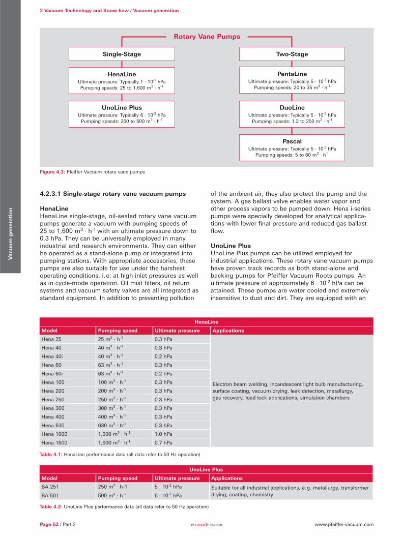
www.pfeiffer-vacuum.comPage 62 / Part 2
2 Vacuum Technology and Know how / Vacuum generationV
acu
um
gen
erat
ion
4.2.3.1 Single-stage rotary vane vacuum pumps
HenaLineHenaLine single-stage, oil-sealed rotary vane vacuum pumps generate a vacuum with pumping speeds of 25 to 1,600 m3 · h-1 with an ultimate pressure down to 0.3 hPa. They can be universally employed in many industrial and research environments. They can either be operated as a stand-alone pump or integrated into pumping stations. With appropriate accessories, these pumps are also suitable for use under the harshest operating conditions, i. e. at high inlet pressures as well as in cycle-mode operation. Oil mist filters, oil return systems and vacuum safety valves are all integrated as standard equipment. In addition to preventing pollution
of the ambient air, they also protect the pump and the system. A gas ballast valve enables water vapor and other process vapors to be pumped down. Hena i-series pumps were specially developed for analytical applica-tions with lower final pressure and reduced gas ballast flow.
UnoLine PlusUnoLine Plus pumps can be utilized employed for industrial applications. These rotary vane vacuum pumps have proven track records as both stand-alone and backing pumps for Pfeiffer Vacuum Roots pumps. An ultimate pressure of approximately 6 · 10-2 hPa can be attained. These pumps are water cooled and extremely insensitive to dust and dirt. They are equipped with an
HenaLine
Model Pumping speed Ultimate pressure Applications
Hena 25 25 m³ · h-1 0.3 hPa
Electron beam welding, incandescent light bulb manufacturing, surface coating, vacuum drying, leak detection, metallurgy, gas recovery, load lock applications, simulation chambers
Hena 40 40 m³ · h-1 0.3 hPa
Hena 40i 40 m³ · h-1 0.2 hPa
Hena 60 63 m³ · h-1 0.3 hPa
Hena 60i 63 m³ · h-1 0.2 hPa
Hena 100 100 m³ · h-1 0.3 hPa
Hena 200 200 m³ · h-1 0.3 hPa
Hena 250 250 m³ · h-1 0.3 hPa
Hena 300 300 m³ · h-1 0.3 hPa
Hena 400 400 m³ · h-1 0.3 hPa
Hena 630 630 m³ · h-1 0.3 hPa
Hena 1000 1,000 m³ · h-1 1.0 hPa
Hena 1600 1,600 m³ · h-1 0.7 hPa
Table 4.1: HenaLine performance data (all data refer to 50 Hz operation)
Figure 4.3: Pfeiffer Vacuum rotary vane pumps
UnoLine Plus
Model Pumping speed Ultimate pressure Applications
BA 251 250 m³ · h-1 5 · 10-2 hPa Suitable for all industrial applications, e. g. metallurgy, transformer drying, coating, chemistryBA 501 500 m³ · h-1 6 · 10-2 hPa
Table 4.2: UnoLine Plus performance data (all data refer to 50 Hz operation)
Rotary Vane Pumps
Single-Stage
HenaLineUltimate pressure: Typically 1 · 10-1 hPaPumping speeds: 25 to 1,600 m3 · h-1
UnoLine PlusUltimate pressure: Typically 6 · 10-2 hPa
Pumping speeds: 250 to 500 m3 · h-1
Two-Stage
PentaLineUltimate pressure: Typically 5 · 10-3 hPa
Pumping speeds: 20 to 35 m3 · h-1
DuoLineUltimate pressure: Typically 5 · 10-3 hPa
Pumping speeds: 1.3 to 250 m3 · h-1
PascalUltimate pressure: Typically 5 · 10-3 hPa
Pumping speeds: 5 to 60 m3 · h-1
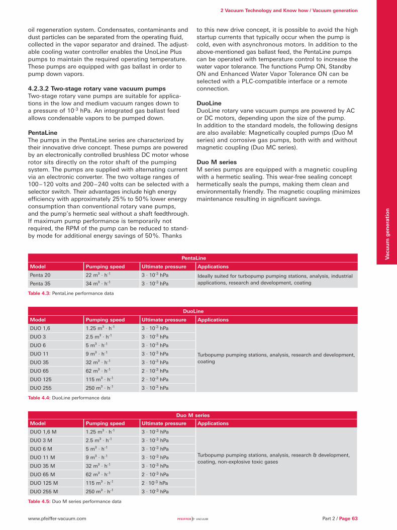
www.pfeiffer-vacuum.com
2 Vacuum Technology and Know how / Vacuum generation
Part 2 / Page 63
Vac
uu
m g
ener
atio
n
oil regeneration system. Condensates, contaminants and dust particles can be separated from the operating fluid, collected in the vapor separator and drained. The adjust-able cooling water controller enables the UnoLine Plus pumps to maintain the required operating temperature. These pumps are equipped with gas ballast in order to pump down vapors.
4.2.3.2 Two-stage rotary vane vacuum pumpsTwo-stage rotary vane pumps are suitable for applica-tions in the low and medium vacuum ranges down to a pressure of 10-3 hPa. An integrated gas ballast feed allows condensable vapors to be pumped down.
PentaLineThe pumps in the PentaLine series are characterized by their innovative drive concept. These pumps are powered by an electronically controlled brushless DC motor whose rotor sits directly on the rotor shaft of the pumping system. The pumps are supplied with alternating current via an electronic converter. The two voltage ranges of 100 – 120 volts and 200 – 240 volts can be selected with a selector switch. Their advantages include high energy efficiency with approximately 25 % to 50 % lower energy consumption than conventional rotary vane pumps, and the pump’s hermetic seal without a shaft feedthrough. If maximum pump performance is temporarily not required, the RPM of the pump can be reduced to stand-by mode for additional energy savings of 50 %. Thanks
to this new drive concept, it is possible to avoid the high startup currents that typically occur when the pump is cold, even with asynchronous motors. In addition to the above-mentioned gas ballast feed, the PentaLine pumps can be operated with temperature control to increase the water vapor tolerance. The functions Pump ON, Standby ON and Enhanced Water Vapor Tolerance ON can be selected with a PLC-compatible interface or a remote connection.
DuoLineDuoLine rotary vane vacuum pumps are powered by AC or DC motors, depending upon the size of the pump. In addition to the standard models, the following designs are also available: Magnetically coupled pumps (Duo M series) and corrosive gas pumps, both with and without magnetic coupling (Duo MC series).
Duo M seriesM series pumps are equipped with a magnetic coupling with a hermetic sealing. This wear-free sealing concept hermetically seals the pumps, making them clean and environmentally friendly. The magnetic coupling minimizes maintenance resulting in significant savings.
PentaLine
Model Pumping speed Ultimate pressure Applications
Penta 20 22 m³ · h-1 3 · 10-3 hPa Ideally suited for turbopump pumping stations, analysis, industrial applications, research and development, coatingPenta 35 34 m³ · h-1 3 · 10-3 hPa
Table 4.3: PentaLine performance data
DuoLine
Model Pumping speed Ultimate pressure Applications
DUO 1,6 1.25 m³ · h-1 3 · 10-3 hPa
Turbopump pumping stations, analysis, research and development, coating
DUO 3 2.5 m³ · h-1 3 · 10-3 hPa
DUO 6 5 m³ · h-1 3 · 10-3 hPa
DUO 11 9 m³ · h-1 3 · 10-3 hPa
DUO 35 32 m³ · h-1 3 · 10-3 hPa
DUO 65 62 m³ · h-1 2 · 10-3 hPa
DUO 125 115 m³ · h-1 2 · 10-3 hPa
DUO 255 250 m³ · h-1 3 · 10-3 hPa
Table 4.4: DuoLine performance data
Duo M series
Model Pumping speed Ultimate pressure Applications
DUO 1,6 M 1.25 m³ · h-1 3 · 10-3 hPa
Turbopump pumping stations, analysis, research & development, coating, non-explosive toxic gases
DUO 3 M 2.5 m³ · h-1 3 · 10-3 hPa
DUO 6 M 5 m³ · h-1 3 · 10-3 hPa
DUO 11 M 9 m³ · h-1 3 · 10-3 hPa
DUO 35 M 32 m³ · h-1 3 · 10-3 hPa
DUO 65 M 62 m³ · h-1 2 · 10-3 hPa
DUO 125 M 115 m³ · h-1 2 . 10-3 hPa
DUO 255 M 250 m³ · h-1 3 · 10-3 hPa
Table 4.5: Duo M series performance data
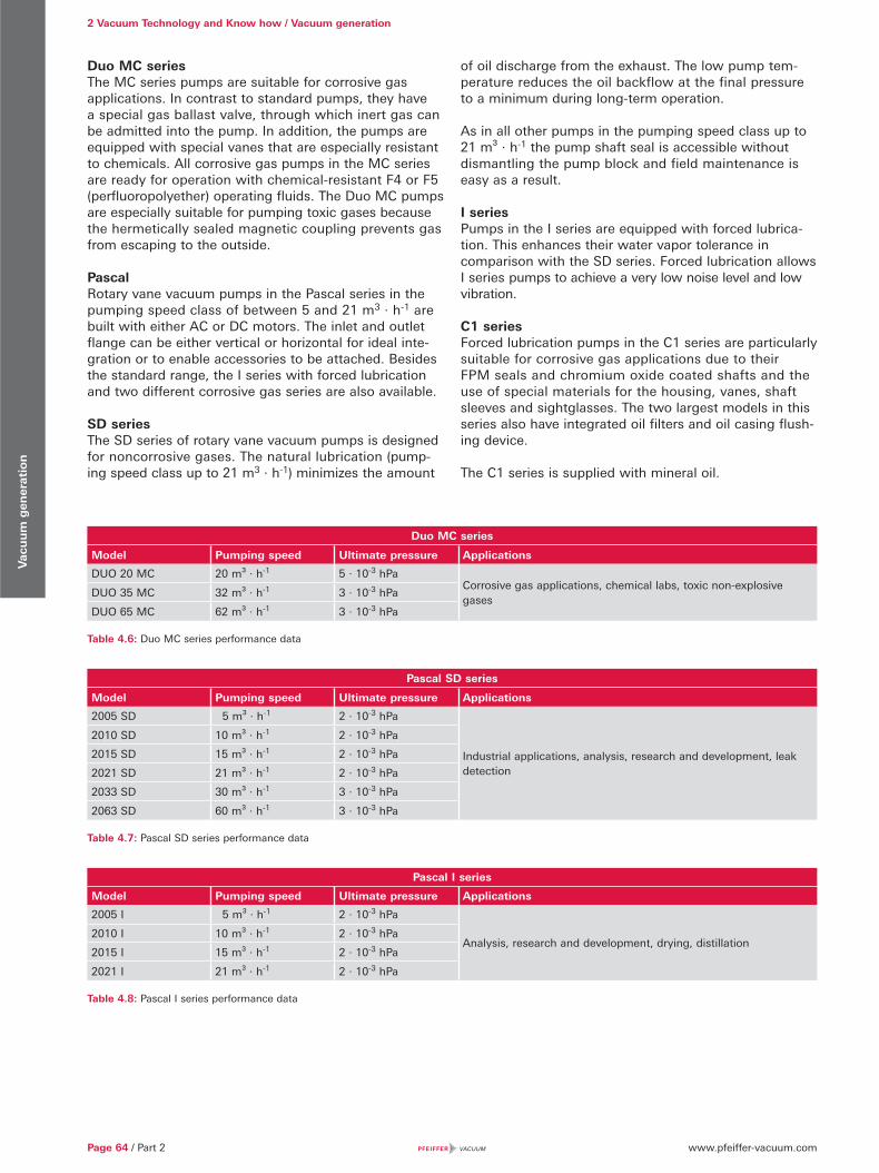
www.pfeiffer-vacuum.comPage 64 / Part 2
2 Vacuum Technology and Know how / Vacuum generationV
acu
um
gen
erat
ion
Duo MC seriesThe MC series pumps are suitable for corrosive gas applications. In contrast to standard pumps, they have a special gas ballast valve, through which inert gas can be admitted into the pump. In addition, the pumps are equipped with special vanes that are especially resistant to chemicals. All corrosive gas pumps in the MC series are ready for operation with chemical-resistant F4 or F5 (perfluoropolyether) operating fluids. The Duo MC pumps are especially suitable for pumping toxic gases because the hermetically sealed magnetic coupling prevents gas from escaping to the outside.
PascalRotary vane vacuum pumps in the Pascal series in the pumping speed class of between 5 and 21 m3 · h-1 are built with either AC or DC motors. The inlet and outlet flange can be either vertical or horizontal for ideal inte-gration or to enable accessories to be attached. Besides the standard range, the I series with forced lubrication and two different corrosive gas series are also available.
SD seriesThe SD series of rotary vane vacuum pumps is designed for noncorrosive gases. The natural lubrication (pump-ing speed class up to 21 m3 · h-1) minimizes the amount
of oil discharge from the exhaust. The low pump tem-perature reduces the oil backflow at the final pressure to a minimum during long-term operation.
As in all other pumps in the pumping speed class up to 21 m³ · h-1 the pump shaft seal is accessible without dismantling the pump block and field maintenance is easy as a result.
I seriesPumps in the I series are equipped with forced lubrica-tion. This enhances their water vapor tolerance in comparison with the SD series. Forced lubrication allows I series pumps to achieve a very low noise level and low vibration.
C1 seriesForced lubrication pumps in the C1 series are particularly suitable for corrosive gas applications due to their FPM seals and chromium oxide coated shafts and the use of special materials for the housing, vanes, shaft sleeves and sightglasses. The two largest models in this series also have integrated oil filters and oil casing flush-ing device.
The C1 series is supplied with mineral oil.
Duo MC series
Model Pumping speed Ultimate pressure Applications
DUO 20 MC 20 m³ · h-1 5 · 10-3 hPaCorrosive gas applications, chemical labs, toxic non-explosive gases
DUO 35 MC 32 m³ · h-1 3 · 10-3 hPa
DUO 65 MC 62 m³ · h-1 3 · 10-3 hPa
Table 4.6: Duo MC series performance data
Pascal SD series
Model Pumping speed Ultimate pressure Applications
2005 SD 5 m³ · h-1 2 · 10-3 hPa
Industrial applications, analysis, research and development, leak detection
2010 SD 10 m³ · h-1 2 · 10-3 hPa
2015 SD 15 m³ · h-1 2 · 10-3 hPa
2021 SD 21 m³ · h-1 2 · 10-3 hPa
2033 SD 30 m³ · h-1 3 · 10-3 hPa
2063 SD 60 m³ · h-1 3 · 10-3 hPa
Table 4.7: Pascal SD series performance data
Pascal I series
Model Pumping speed Ultimate pressure Applications
2005 I 5 m³ · h-1 2 · 10-3 hPa
Analysis, research and development, drying, distillation 2010 I 10 m³ · h-1 2 · 10-3 hPa
2015 I 15 m³ · h-1 2 · 10-3 hPa
2021 I 21 m³ · h-1 2 · 10-3 hPa
Table 4.8: Pascal I series performance data
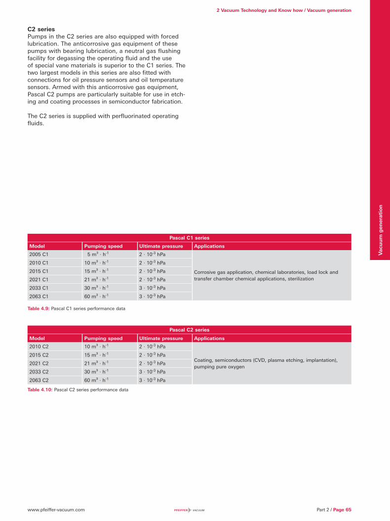
www.pfeiffer-vacuum.com
2 Vacuum Technology and Know how / Vacuum generation
Part 2 / Page 65
Vac
uu
m g
ener
atio
n
C2 seriesPumps in the C2 series are also equipped with forced lubrication. The anticorrosive gas equipment of these pumps with bearing lubrication, a neutral gas flushing facility for degassing the operating fluid and the use of special vane materials is superior to the C1 series. The two largest models in this series are also fitted with connections for oil pressure sensors and oil temperature sensors. Armed with this anticorrosive gas equipment, Pascal C2 pumps are particularly suitable for use in etch-ing and coating processes in semiconductor fabrication.
The C2 series is supplied with perfluorinated operating fluids.
Pascal C1 series
Model Pumping speed Ultimate pressure Applications
2005 C1 5 m³ · h-1 2 · 10-3 hPa
Corrosive gas application, chemical laboratories, load lock and transfer chamber chemical applications, sterilization
2010 C1 10 m³ · h-1 2 · 10-3 hPa
2015 C1 15 m³ · h-1 2 · 10-3 hPa
2021 C1 21 m³ · h-1 2 · 10-3 hPa
2033 C1 30 m³ · h-1 3 · 10-3 hPa
2063 C1 60 m³ · h-1 3 · 10-3 hPa
Table 4.9: Pascal C1 series performance data
Pascal C2 series
Model Pumping speed Ultimate pressure Applications
2010 C2 10 m³ · h-1 2 · 10-3 hPa
Coating, semiconductors (CVD, plasma etching, implantation), pumping pure oxygen
2015 C2 15 m³ · h-1 2 · 10-3 hPa
2021 C2 21 m³ · h-1 2 · 10-3 hPa
2033 C2 30 m³ · h-1 3 · 10-3 hPa
2063 C2 60 m³ · h-1 3 · 10-3 hPa
Table 4.10: Pascal C2 series performance data
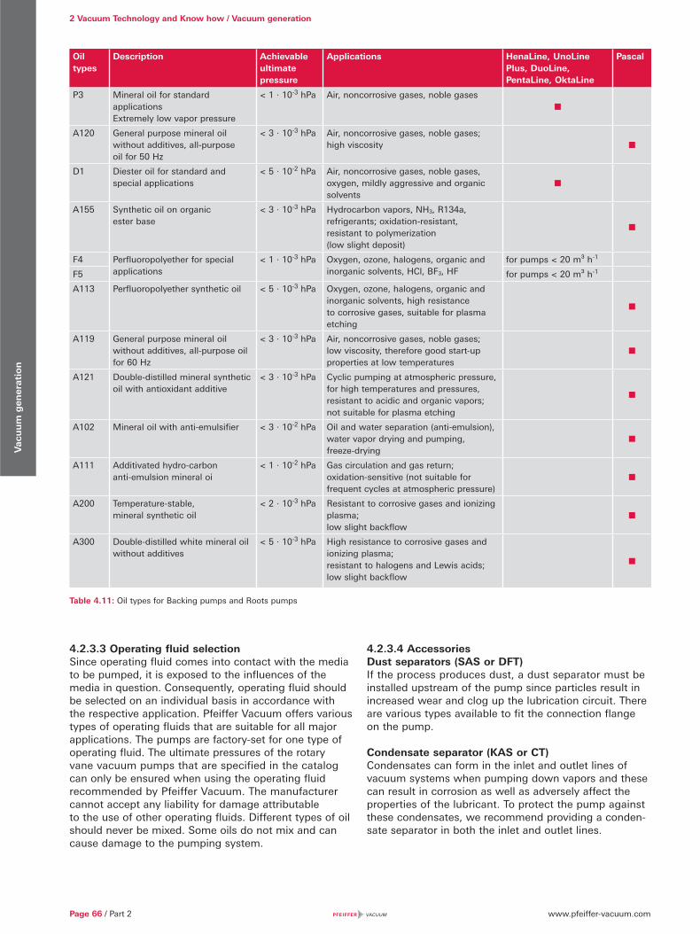
www.pfeiffer-vacuum.comPage 66 / Part 2
2 Vacuum Technology and Know how / Vacuum generationV
acu
um
gen
erat
ion
Oil types
Description Achievable ultimate pressure
Applications HenaLine, UnoLine Plus, DuoLine, PentaLine, OktaLine
Pascal
P3 Mineral oil for standard applicationsExtremely low vapor pressure
< 1 · 10-3 hPa Air, noncorrosive gases, noble gases
A120 General purpose mineral oil without additives, all-purpose oil for 50 Hz
< 3 · 10-3 hPa Air, noncorrosive gases, noble gases;high viscosity
D1 Diester oil for standard and special applications
< 5 · 10-2 hPa Air, noncorrosive gases, noble gases, oxygen, mildly aggressive and organic solvents
A155 Synthetic oil on organic ester base
< 3 · 10-3 hPa Hydrocarbon vapors, NH3, R134a, refrigerants; oxidation-resistant,resistant to polymerization (low slight deposit)
F4 Perfluoropolyether for special applications
< 1 · 10-3 hPa Oxygen, ozone, halogens, organic and inorganic solvents, HCl, BF3, HF
for pumps < 20 m³ h-1
F5 for pumps < 20 m³ h-1
A113 Perfluoropolyether synthetic oil < 5 · 10-3 hPa Oxygen, ozone, halogens, organic and inorganic solvents, high resistance to corrosive gases, suitable for plasma etching
A119 General purpose mineral oil without additives, all-purpose oil for 60 Hz
< 3 · 10-3 hPa Air, noncorrosive gases, noble gases;low viscosity, therefore good start-up properties at low temperatures
A121 Double-distilled mineral synthetic oil with antioxidant additive
< 3 · 10-3 hPa Cyclic pumping at atmospheric pressure, for high temperatures and pressures, resistant to acidic and organic vapors;not suitable for plasma etching
A102 Mineral oil with anti-emulsifier < 3 · 10-2 hPa Oil and water separation (anti-emulsion), water vapor drying and pumping, freeze-drying
A111 Additivated hydro-carbon anti-emulsion mineral oi
< 1 · 10-2 hPa Gas circulation and gas return;oxidation-sensitive (not suitable for frequent cycles at atmospheric pressure)
A200 Temperature-stable, mineral synthetic oil
< 2 · 10-3 hPa Resistant to corrosive gases and ionizing plasma; low slight backflow
A300 Double-distilled white mineral oil without additives
< 5 · 10-3 hPa High resistance to corrosive gases and ionizing plasma;resistant to halogens and Lewis acids;low slight backflow
Table 4.11: Oil types for Backing pumps and Roots pumps
4.2.3.3 Operating fluid selectionSince operating fluid comes into contact with the media to be pumped, it is exposed to the influences of the media in question. Consequently, operating fluid should be selected on an individual basis in accordance with the respective application. Pfeiffer Vacuum offers various types of operating fluids that are suitable for all major applications. The pumps are factory-set for one type of operating fluid. The ultimate pressures of the rotary vane vacuum pumps that are specified in the catalog can only be ensured when using the operating fluid recommended by Pfeiffer Vacuum. The manufacturer cannot accept any liability for damage attributable to the use of other operating fluids. Different types of oil should never be mixed. Some oils do not mix and can cause damage to the pumping system.
4.2.3.4 AccessoriesDust separators (SAS or DFT)If the process produces dust, a dust separator must be installed upstream of the pump since particles result in increased wear and clog up the lubrication circuit. There are various types available to fit the connection flange on the pump.
Condensate separator (KAS or CT)Condensates can form in the inlet and outlet lines of vacuum systems when pumping down vapors and these can result in corrosion as well as adversely affect the properties of the lubricant. To protect the pump against these condensates, we recommend providing a conden-sate separator in both the inlet and outlet lines.
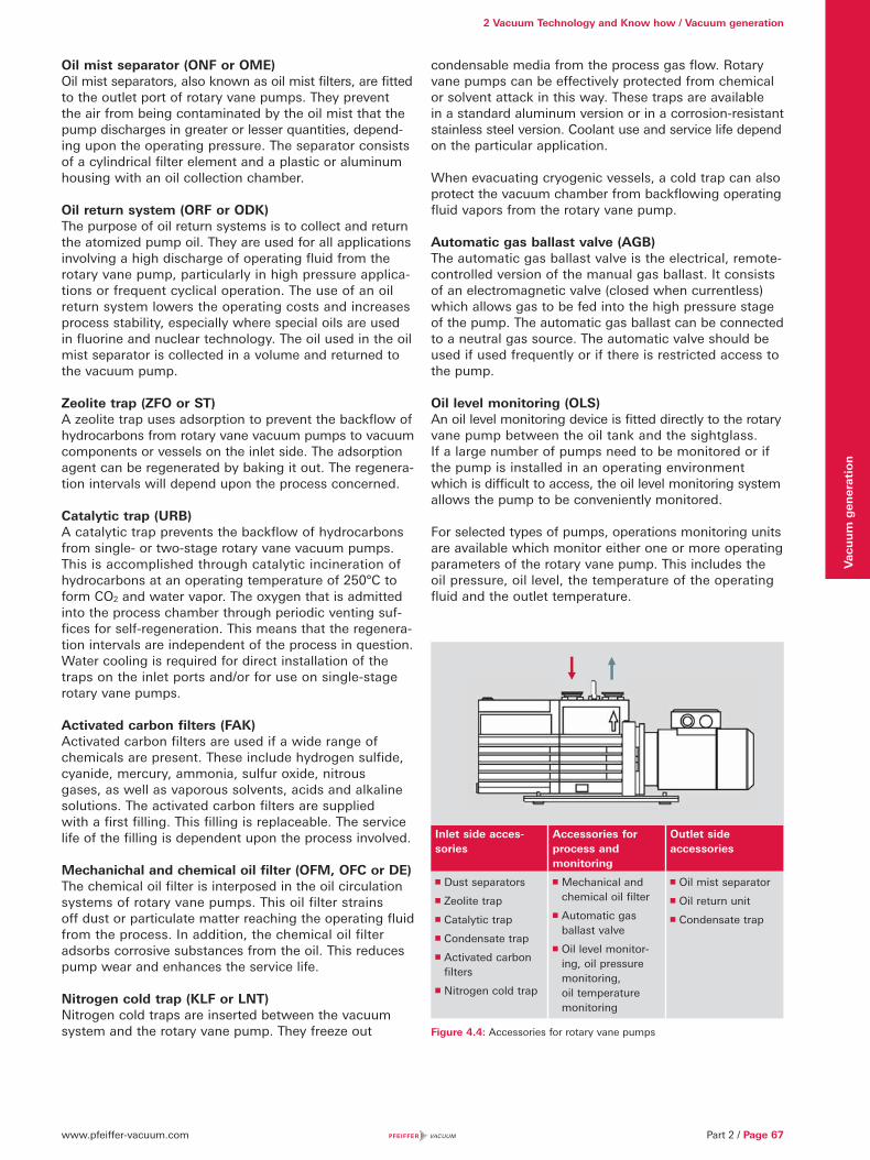
www.pfeiffer-vacuum.com
2 Vacuum Technology and Know how / Vacuum generation
Part 2 / Page 67
Vac
uu
m g
ener
atio
n
Oil mist separator (ONF or OME)Oil mist separators, also known as oil mist filters, are fitted to the outlet port of rotary vane pumps. They prevent the air from being contaminated by the oil mist that the pump discharges in greater or lesser quantities, depend-ing upon the operating pressure. The separator consists of a cylindrical filter element and a plastic or aluminum housing with an oil collection chamber.
Oil return system (ORF or ODK)The purpose of oil return systems is to collect and return the atomized pump oil. They are used for all applications involving a high discharge of operating fluid from the rotary vane pump, particularly in high pressure applica-tions or frequent cyclical operation. The use of an oil return system lowers the operating costs and increases process stability, especially where special oils are used in fluorine and nuclear technology. The oil used in the oil mist separator is collected in a volume and returned to the vacuum pump.
Zeolite trap (ZFO or ST)A zeolite trap uses adsorption to prevent the backflow of hydrocarbons from rotary vane vacuum pumps to vacuum components or vessels on the inlet side. The adsorption agent can be regenerated by baking it out. The regenera-tion intervals will depend upon the process concerned.
Catalytic trap (URB)A catalytic trap prevents the backflow of hydrocarbons from single- or two-stage rotary vane vacuum pumps. This is accomplished through catalytic incineration of hydrocarbons at an operating temperature of 250°C to form CO2 and water vapor. The oxygen that is admittedinto the process chamber through periodic venting suf-fices for self-regeneration. This means that the regenera-tion intervals are independent of the process in question. Water cooling is required for direct installation of the traps on the inlet ports and/or for use on single-stage rotary vane pumps.
Activated carbon filters (FAK)Activated carbon filters are used if a wide range of chemicals are present. These include hydrogen sulfide, cyanide, mercury, ammonia, sulfur oxide, nitrous gases, as well as vaporous solvents, acids and alkaline solutions. The activated carbon filters are supplied with a first filling. This filling is replaceable. The service life of the filling is dependent upon the process involved.
Mechanichal and chemical oil filter (OFM, OFC or DE)The chemical oil filter is interposed in the oil circulation systems of rotary vane pumps. This oil filter strains off dust or particulate matter reaching the operating fluid from the process. In addition, the chemical oil filter adsorbs corrosive substances from the oil. This reduces pump wear and enhances the service life.
Nitrogen cold trap (KLF or LNT)Nitrogen cold traps are inserted between the vacuum system and the rotary vane pump. They freeze out
condensable media from the process gas flow. Rotary vane pumps can be effectively protected from chemical or solvent attack in this way. These traps are available in a standard aluminum version or in a corrosion-resistant stainless steel version. Coolant use and service life depend on the particular application.
When evacuating cryogenic vessels, a cold trap can also protect the vacuum chamber from backflowing operating fluid vapors from the rotary vane pump.
Automatic gas ballast valve (AGB)The automatic gas ballast valve is the electrical, remote-controlled version of the manual gas ballast. It consists of an electromagnetic valve (closed when currentless) which allows gas to be fed into the high pressure stage of the pump. The automatic gas ballast can be connected to a neutral gas source. The automatic valve should be used if used frequently or if there is restricted access to the pump.
Oil level monitoring (OLS)An oil level monitoring device is fitted directly to the rotary vane pump between the oil tank and the sightglass. If a large number of pumps need to be monitored or if the pump is installed in an operating environment which is difficult to access, the oil level monitoring system allows the pump to be conveniently monitored.
For selected types of pumps, operations monitoring units are available which monitor either one or more operating parameters of the rotary vane pump. This includes the oil pressure, oil level, the temperature of the operating fluid and the outlet temperature.
Figure 4.4: Accessories for rotary vane pumps
Inlet side acces-sories
Accessories for process and monitoring
Outlet side accessories
Dust separators
Zeolite trap
Catalytic trap
Condensate trap
Activated carbon filters
Nitrogen cold trap
Mechanical and chemical oil filter
Automatic gas ballast valve
Oil level monitor-ing, oil pressure monitoring, oil temperature monitoring
Oil mist separator
Oil return unit
Condensate trap
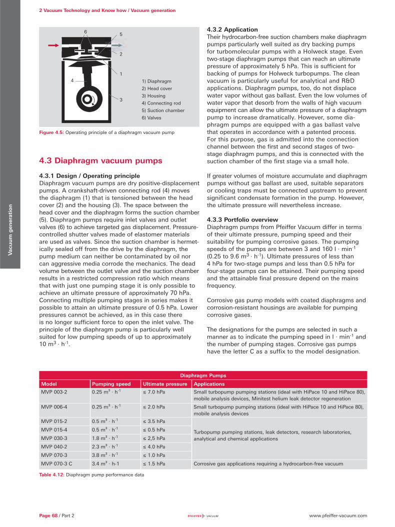
www.pfeiffer-vacuum.comPage 68 / Part 2
2 Vacuum Technology and Know how / Vacuum generationV
acu
um
gen
erat
ion
4.3 Diaphragm vacuum pumps
4.3.1 Design / Operating principleDiaphragm vacuum pumps are dry positive-displacement pumps. A crankshaft-driven connecting rod (4) moves the diaphragm (1) that is tensioned between the head cover (2) and the housing (3). The space between the head cover and the diaphragm forms the suction chamber (5). Diaphragm pumps require inlet valves and outlet valves (6) to achieve targeted gas displacement. Pressure-controlled shutter valves made of elastomer materials are used as valves. Since the suction chamber is hermet-ically sealed off from the drive by the diaphragm, the pump medium can neither be contaminated by oil nor can aggressive media corrode the mechanics. The dead volume between the outlet valve and the suction chamber results in a restricted compression ratio which means that with just one pumping stage it is only possible to achieve an ultimate pressure of approximately 70 hPa. Connecting multiple pumping stages in series makes it possible to attain an ultimate pressure of 0.5 hPa. Lower pressures cannot be achieved, as in this case there is no longer sufficient force to open the inlet valve. The principle of the diaphragm pump is particularly well suited for low pumping speeds of up to approximately 10 m3 · h-1.
4.3.2 ApplicationTheir hydrocarbon-free suction chambers make diaphragm pumps particularly well suited as dry backing pumps for turbomolecular pumps with a Holweck stage. Even two-stage diaphragm pumps that can reach an ultimate pressure of approximately 5 hPa. This is sufficient for backing of pumps for Holweck turbopumps. The clean vacuum is particularly useful for analytical and R&D applications. Diaphragm pumps, too, do not displace water vapor without gas ballast. Even the low volumes of water vapor that desorb from the walls of high vacuum equipment can allow the ultimate pressure of a diaphragm pump to increase dramatically. However, some dia-phragm pumps are equipped with a gas ballast valve that operates in accordance with a patented process. For this purpose, gas is admitted into the connection channel between the first and second stages of two-stage diaphragm pumps, and this is connected with the suction chamber of the first stage via a small hole.
If greater volumes of moisture accumulate and diaphragm pumps without gas ballast are used, suitable separators or cooling traps must be connected upstream to prevent significant condensate formation in the pump. However, the ultimate pressure will nevertheless increase.
4.3.3 Portfolio overviewDiaphragm pumps from Pfeiffer Vacuum differ in terms of their ultimate pressure, pumping speed and their suitability for pumping corrosive gases. The pumping speeds of the pumps are between 3 and 160 l · min-1 (0.25 to 9.6 m3 · h-1). Ultimate pressures of less than 4 hPa for two-stage pumps and less than 0.5 hPa for four-stage pumps can be attained. Their pumping speed and the attainable final pressure depend on the mains frequency.
Corrosive gas pump models with coated diaphragms and corrosion-resistant housings are available for pumping corrosive gases.
The designations for the pumps are selected in such a manner as to indicate the pumping speed in l · min-1 and the number of pumping stages. Corrosive gas pumps have the letter C as a suffix to the model designation.
Diaphragm Pumps
Model Pumping speed Ultimate pressure Applications
MVP 003-2 0.25 m³ · h-1 ≤ 7.0 hPa Small turbopump pumping stations (ideal with HiPace 10 and HiPace 80),mobile analysis devices, Minitest helium leak detector regeneration
MVP 006-4 0.25 m³ · h-1 ≤ 2.0 hPa Small turbopump pumping stations (ideal with HiPace 10 and HiPace 80), mobile analysis devices
MVP 015-2 0.5 m³ · h-1 ≤ 3.5 hPa
Turbopump pumping stations, leak detectors, research laboratories, analytical and chemical applications
MVP 015-4 0.5 m³ · h-1 ≤ 0.5 hPa
MVP 030-3 1.8 m³ · h-1 ≤ 2,5 hPa
MVP 040-2 2.3 m³ · h-1 ≤ 4.0 hPa
MVP 070-3 3.8 m³ · h-1 ≤ 1.0 hPa
MVP 070-3 C 3.4 m³ · h-1 ≤ 1.5 hPa Corrosive gas applications requiring a hydrocarbon-free vacuum
Table 4.12: Diaphragm pump performance data
Figure 4.5: Operating principle of a diaphragm vacuum pump
1) Diaphragm
2) Head cover
3) Housing
4) Connecting rod
5) Suction chamber
6) Valves
5
2
1
3
6
4
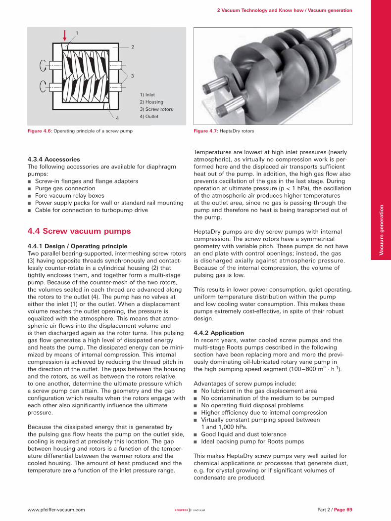
www.pfeiffer-vacuum.com
2 Vacuum Technology and Know how / Vacuum generation
Part 2 / Page 69
Vac
uu
m g
ener
atio
n
4.3.4 AccessoriesThe following accessories are available for diaphragm pumps:
Screw-in flanges and flange adapters Purge gas connection Fore-vacuum relay boxes Power supply packs for wall or standard rail mounting Cable for connection to turbopump drive
4.4 Screw vacuum pumps
4.4.1 Design / Operating principleTwo parallel bearing-supported, intermeshing screw rotors (3) having opposite threads synchronously and contact-lessly counter-rotate in a cylindrical housing (2) that tightly encloses them, and together form a multi-stage pump. Because of the counter-mesh of the two rotors, the volumes sealed in each thread are advanced along the rotors to the outlet (4). The pump has no valves at either the inlet (1) or the outlet. When a displacement volume reaches the outlet opening, the pressure is equalized with the atmosphere. This means that atmo-spheric air flows into the displacement volume and is then discharged again as the rotor turns. This pulsing gas flow generates a high level of dissipated energy and heats the pump. The dissipated energy can be mini-mized by means of internal compression. This internal compression is achieved by reducing the thread pitch in the direction of the outlet. The gaps between the housing and the rotors, as well as between the rotors relative to one another, determine the ultimate pressure which a screw pump can attain. The geometry and the gap configuration which results when the rotors engage with each other also significantly influence the ultimate pressure.
Because the dissipated energy that is generated by the pulsing gas flow heats the pump on the outlet side, cooling is required at precisely this location. The gap between housing and rotors is a function of the temper-ature differential between the warmer rotors and the cooled housing. The amount of heat produced and the temperature are a function of the inlet pressure range.
Temperatures are lowest at high inlet pressures (nearly atmospheric), as virtually no compression work is per-formed here and the displaced air transports sufficient heat out of the pump. In addition, the high gas flow also prevents oscillation of the gas in the last stage. During operation at ultimate pressure (p < 1 hPa), the oscillation of the atmospheric air produces higher temperatures at the outlet area, since no gas is passing through the pump and therefore no heat is being transported out of the pump.
HeptaDry pumps are dry screw pumps with internal compression. The screw rotors have a symmetrical geometry with variable pitch. These pumps do not have an end plate with control openings; instead, the gas is discharged axially against atmospheric pressure. Because of the internal compression, the volume of pulsing gas is low.
This results in lower power consumption, quiet operating, uniform temperature distribution within the pump and low cooling water consumption. This makes these pumps extremely cost-effective, in spite of their robust design.
4.4.2 Application In recent years, water cooled screw pumps and the multi-stage Roots pumps described in the following section have been replacing more and more the previ-ously dominating oil-lubricated rotary vane pump in the high pumping speed segment (100 – 600 m³ · h-1).
Advantages of screw pumps include: No lubricant in the gas displacement area No contamination of the medium to be pumped No operating fluid disposal problems Higher efficiency due to internal compression Virtually constant pumping speed between
1 and 1,000 hPa. Good liquid and dust tolerance Ideal backing pump for Roots pumps
This makes HeptaDry screw pumps very well suited for chemical applications or processes that generate dust, e. g. for crystal growing or if significant volumes of condensate are produced.
Figure 4.6: Operating principle of a screw pump Figure 4.7: HeptaDry rotors
1) Inlet
2) Housing
3) Screw rotors
4) Outlet
1
2
3
4
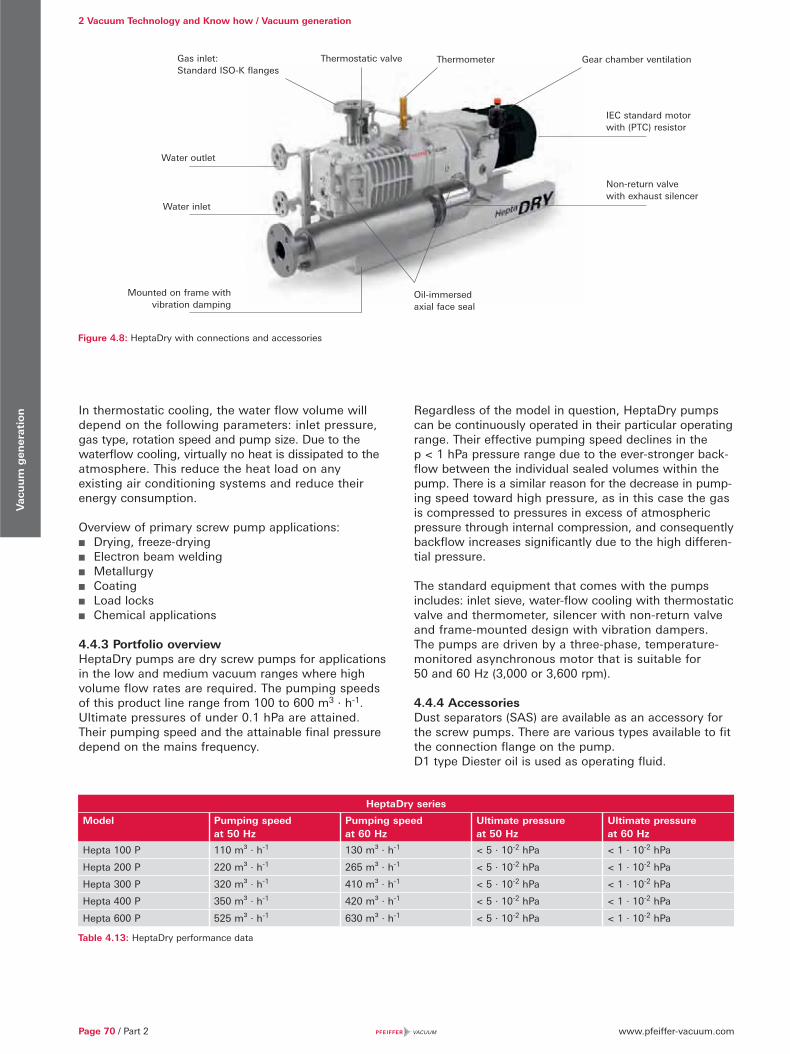
www.pfeiffer-vacuum.comPage 70 / Part 2
2 Vacuum Technology and Know how / Vacuum generationV
acu
um
gen
erat
ion In thermostatic cooling, the water flow volume will
depend on the following parameters: inlet pressure, gas type, rotation speed and pump size. Due to the waterflow cooling, virtually no heat is dissipated to the atmosphere. This reduce the heat load on any existing air conditioning systems and reduce their energy consumption.
Overview of primary screw pump applications: Drying, freeze-drying Electron beam welding Metallurgy Coating Load locks Chemical applications
4.4.3 Portfolio overviewHeptaDry pumps are dry screw pumps for applications in the low and medium vacuum ranges where high volume flow rates are required. The pumping speeds of this product line range from 100 to 600 m3 · h-1. Ultimate pressures of under 0.1 hPa are attained. Their pumping speed and the attainable final pressure depend on the mains frequency.
HeptaDry series
Model Pumping speed at 50 Hz
Pumping speed at 60 Hz
Ultimate pressure at 50 Hz
Ultimate pressure at 60 Hz
Hepta 100 P 110 m³ · h-1 130 m³ · h-1 < 5 · 10-2 hPa < 1 · 10-2 hPa
Hepta 200 P 220 m³ · h-1 265 m³ · h-1 < 5 · 10-2 hPa < 1 · 10-2 hPa
Hepta 300 P 320 m³ · h-1 410 m³ · h-1 < 5 · 10-2 hPa < 1 · 10-2 hPa
Hepta 400 P 350 m³ · h-1 420 m³ · h-1 < 5 · 10-2 hPa < 1 · 10-2 hPa
Hepta 600 P 525 m³ · h-1 630 m³ · h-1 < 5 · 10-2 hPa < 1 · 10-2 hPa
Table 4.13: HeptaDry performance data
Figure 4.8: HeptaDry with connections and accessories
Regardless of the model in question, HeptaDry pumps can be continuously operated in their particular operating range. Their effective pumping speed declines in the p < 1 hPa pressure range due to the ever-stronger back-flow between the individual sealed volumes within the pump. There is a similar reason for the decrease in pump-ing speed toward high pressure, as in this case the gas is compressed to pressures in excess of atmospheric pressure through internal compression, and consequently backflow increases significantly due to the high differen-tial pressure.
The standard equipment that comes with the pumps includes: inlet sieve, water-flow cooling with thermostatic valve and thermometer, silencer with non-return valve and frame-mounted design with vibration dampers. The pumps are driven by a three-phase, temperature-monitored asynchronous motor that is suitable for 50 and 60 Hz (3,000 or 3,600 rpm).
4.4.4 AccessoriesDust separators (SAS) are available as an accessory for the screw pumps. There are various types available to fit the connection flange on the pump.D1 type Diester oil is used as operating fluid.
IEC standard motorwith (PTC) resistor
Non-return valvewith exhaust silencer
Water outlet
Water inlet
Oil-immersedaxial face seal
Thermometer Gear chamber ventilationGas inlet: Standard ISO-K flanges
Thermostatic valve
Mounted on frame with vibration damping
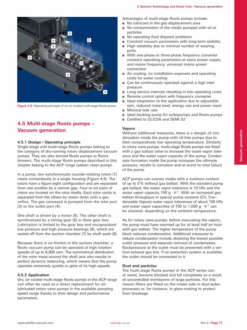
www.pfeiffer-vacuum.com
2 Vacuum Technology and Know how / Vacuum generation
Part 2 / Page 71
Vac
uu
m g
ener
atio
n
4.5 Multi-stage Roots pumps – Vacuum generation
4.5.1 Design / Operating principleSingle-stage and multi-stage Roots pumps belong to the category of dry-running rotary displacement vacuum pumps. They are also termed Roots pumps or Roots blowers. The multi-stage Roots pumps described in this chapter belong to the ACP range (adixen clean pump).
In a pump, two synchronously counter-rotating rotors (1) rotate contactlessly in a single housing (Figure 4.9). The rotors have a figure-eight configuration and are separated from one another by a narrow gap. Four to six pairs of rotors are located on the rotor shafts. Each rotor cavity is separated from the others by stator disks with a gas orifice. The gas conveyed is pumped from the inlet port (3) to the outlet port (4).
One shaft is driven by a motor (5). The other shaft is synchronized by a timing gear (6) in thew gear box. Lubrication is limited to the gear box and encapsulated low pressure and high pressure bearings (9), which are sealed off from the suction chamber (7) by shaft seals (8).
Because there is no friction in the suction chamber, a Roots vacuum pump can be operated at high rotation speeds of up to 6,000 rpm. The symmetrical distribution of the rotor mass around the shaft axis also results in perfect dynamic balancing, which means that the pump operates extremely quietly in spite of its high speeds.
4.5.2 ApplicationDry, air cooled multi-stage Roots pumps in the ACP range can often be used as a direct replacement for oil- lubricated rotary vane pumps in the available pumping speed range thanks to their design and performance parameters.
Advantages of multi-stage Roots pumps include: No lubricant in the gas displacement area No contamination of the media pumped with oil or
particles No operating fluid disposal problems Constant vacuum parameters with long-term stability High reliability due to minimal number of wearing
parts With one-phase or three-phase frequency converter
constant operating parameters at every power supply and mains frequency, universal mains power connection
Air cooling, no installation expenses and operating costs for water cooling
Can be continuously operated against a high inlet pressure
Long service intervals resulting in low operating costs Remote control option with frequency converter Ideal adaptation to the application due to adjustable
rpm, reduced noise level, energy use and power input Minimal leak rate Ideal backing pump for turbopumps and Roots pumps Certified to UL/CSA and SEMI S2
VaporsWithout additional measures, there is a danger of con-densation inside the pump with oil-free pumps due to their comparatively low operating temperature. Similarly to rotary vane pumps, multi-stage Roots pumps are fitted with a gas ballast valve to increase the water vapor toler-ance and the water vapor capacity of the pump. Conden-sate formation inside the pump increases the ultimate pressure, results in corrosion and at worst to total failure of the pump.
ACP pumps can convey media with a moisture content of up to 5 % without gas ballast. With the standard pump gas ballast, the water vapor tolerance is 10 hPa and the water vapor capacity 100 g · h-1. With an increased gas ballast throughput in special pump versions (CV, Con-densable Vapors) water vapor tolerances of about 100 hPa and water vapor capacities of 700 to 1,000 g · h-1 can be attained, depending on the ambient temperature.
As for rotary vane pumps: before evacuating the vapors, the pump must have warmed up for at least half an hour with gas ballast. The higher temperature of the pump block reduces condensation. Additional measures to reduce condensation include obtaining the lowest possible outlet pressure and separate removal of condensates. Backpressure at the outlet must be prevented with a ver-tical exhaust gas line. If an extraction system is available, the outlet should be connected to it.
Dust and particlesThe multi-stage Roots pumps in the ACP series can, at worst, become blocked and fail completely as a result of uncontrolled immissions of large particles. For this reason filters are fitted on the intake side in dust-laden processes or, for instance, in glass-making to protect from breakage.
Figure 4.9: Operating principle of an air cooled multi-stage Roots pump
1
2
3
4
5
6
7
8
9
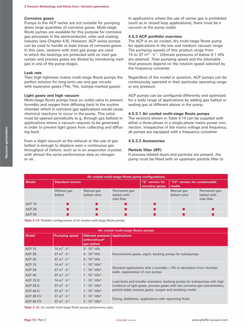
www.pfeiffer-vacuum.comPage 72 / Part 2
2 Vacuum Technology and Know how / Vacuum generationV
acu
um
gen
erat
ion
Corrosive gasesPumps in the ACP series are not suitable for pumping down large quantities of corrosive gases. Multi-stage Roots pumps are available for this purpose for corrosive gas processes in the semiconductor, solar and coating industry (see Chapter 4.6). However, ACP series pumps can be used to handle at least traces of corrosive gases. In this case, versions with inert gas purge are used in which the bearings are protected with an inert gas curtain and process gases are diluted by introducing inert gas in one of the pump stages.
Leak rateTheir high tightness makes multi-stage Roots pumps the perfect solution for long-term use and gas circuits with expensive gases (4He, 3He, isotope-marked gases).
Light gases and high vacuumMulti-stage Roots pumps have an outlet valve to prevent humidity and oxygen from diffusing back to the suction chamber which in corrosive gas applications would cause chemical reactions to occur in the pump. This valve must be opened periodically (e. g. through gas ballast) in applications where a vacuum requires to be generated in order to prevent light gases from collecting and diffus-ing back.
Even a slight vacuum at the exhaust or the use of gas ballast is enough to displace even a continuous gas throughput of helium, such as in an evaporator cryostat, with almost the same performance data as nitrogen or air.
In applications where the use of carrier gas is prohibited (such as in closed loop applications), there must be a vacuum at the pump outlet.
4.5.3 ACP portfolio overview The ACP is an air cooled, dry multi-stage Roots pump for applications in the low and medium vacuum range. The pumping speeds of this product range from 14 to 37 m3 · h-1. Ultimate pressures of below 0.1 hPa are attained. Their pumping speed and the attainable final pressure depend on the rotation speed selected by the frequency converter.
Regardless of the model in question, ACP pumps can be continuously operated in their particular operating range at any pressure.
ACP pumps can be configured differently and optimized for a wide range of applications by adding gas ballast or sealing gas at different places in the pump.
4.5.3.1 Air cooled multi-stage Roots pumps The versions shown in Table 4.14 can be supplied with either a three-phase or a single-phase mains power con-nection. Irrespective of the mains voltage and frequency, all pumps are equipped with a frequency converter.
4.5.3.2 Accessories
Particle filter (IPF)If process-related dusts and particles are present, the pump must be fitted with an upstream particle filter to
Air cooled multi-stage Roots pump configurations
Model Standard version ”G“ version for corrosive gases
”CV“ version for condensable media
Without gas ballast
Manual gas ballast valve
Permanent gas ballast with inlet filter
Manual gas ballast valve
Permanent gas ballast with inlet filter
ACP 15
ACP 28
ACP 40
Table 4.14: Possible configurations of air cooled multi-stage Roots pumps
Air cooled multi-stage Roots pumps
Model Pumping speed Ultimate pressure with/without* gas ballast
Applications
ACP 15 14 m³ · h-1 3 · 10-2 hPa
Noncorrosive gases, argon, backing pumps for turbopumpsACP 28 27 m³ · h-1 3 · 10-2 hPa
ACP 40 37 m³ · h-1 3 · 10-2 hPa
ACP 15 14 m³ · h-1 1 · 10-1 hPa*Standard applications with a humidity > 5% or desorption from chamber walls, regeneration of cryo pumps
ACP 28 27 m³ · h-1 1 · 10-1 hPa*
ACP 40 37 m³ · h-1 1 · 10-1 hPa*
ACP 15 G 14 m³ · h-1 1 · 10-1 hPa* Load locks and transfer chambers, backing pumps for turbopumps with high incidence of light gases, process gases with low corrosive gas concentration, particle-laden process gases, oxygen and oxidating media
ACP 28 G 27 m³ · h-1 1 · 10-1 hPa*
ACP 40 G 37 m³ · h-1 1 · 10-1 hPa*
ACP 28 CV 27 m³ · h-1 2 · 10-1 hPa*Drying, distillation, applications with vaporizing fluids
ACP 40 CV 37 m³ · h-1 2 · 10-1 hPa*
Table 4.15: Air cooled multi-stage Roots pump performance data
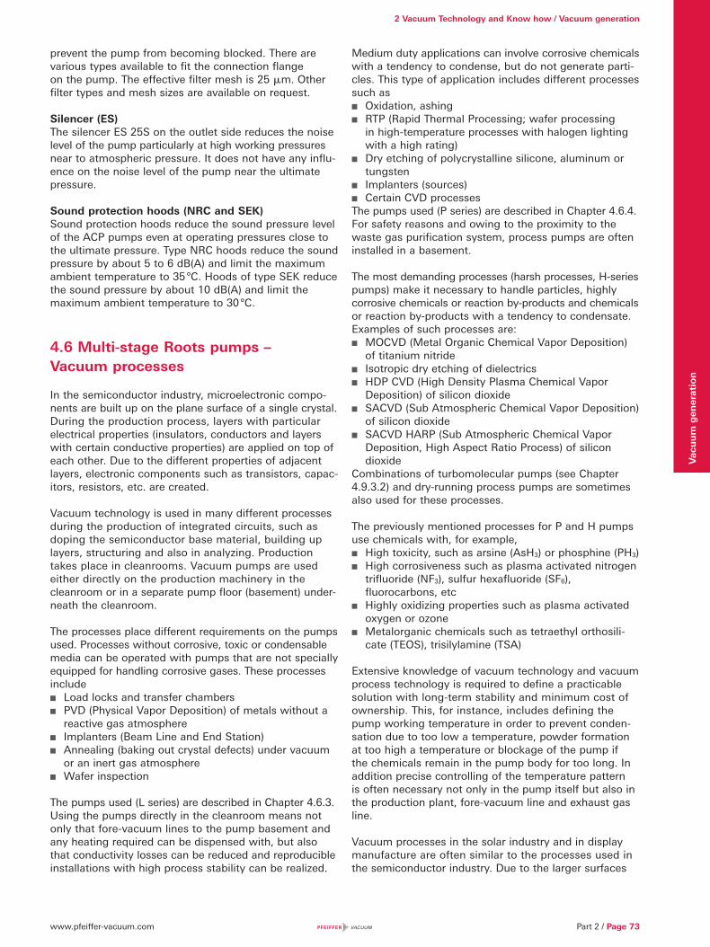
www.pfeiffer-vacuum.com
2 Vacuum Technology and Know how / Vacuum generation
Part 2 / Page 73
Vac
uu
m g
ener
atio
n
prevent the pump from becoming blocked. There are various types available to fit the connection flange on the pump. The effective filter mesh is 25 �m. Other filter types and mesh sizes are available on request.
Silencer (ES)The silencer ES 25S on the outlet side reduces the noise level of the pump particularly at high working pressures near to atmospheric pressure. It does not have any influ-ence on the noise level of the pump near the ultimate pressure.
Sound protection hoods (NRC and SEK)Sound protection hoods reduce the sound pressure level of the ACP pumps even at operating pressures close to the ultimate pressure. Type NRC hoods reduce the sound pressure by about 5 to 6 dB(A) and limit the maximum ambient temperature to 35 °C. Hoods of type SEK reduce the sound pressure by about 10 dB(A) and limit the maximum ambient temperature to 30 °C.
4.6 Multi-stage Roots pumps – Vacuum processes
In the semiconductor industry, microelectronic compo-nents are built up on the plane surface of a single crystal. During the production process, layers with particular electrical properties (insulators, conductors and layers with certain conductive properties) are applied on top of each other. Due to the different properties of adjacent layers, electronic components such as transistors, capac-itors, resistors, etc. are created.
Vacuum technology is used in many different processes during the production of integrated circuits, such as doping the semiconductor base material, building up layers, structuring and also in analyzing. Production takes place in cleanrooms. Vacuum pumps are used either directly on the production machinery in the cleanroom or in a separate pump floor (basement) under-neath the cleanroom.
The processes place different requirements on the pumps used. Processes without corrosive, toxic or condensable media can be operated with pumps that are not specially equipped for handling corrosive gases. These processes include
Load locks and transfer chambers PVD (Physical Vapor Deposition) of metals without a
reactive gas atmosphere Implanters (Beam Line and End Station) Annealing (baking out crystal defects) under vacuum
or an inert gas atmosphere Wafer inspection
The pumps used (L series) are described in Chapter 4.6.3. Using the pumps directly in the cleanroom means not only that fore-vacuum lines to the pump basement and any heating required can be dispensed with, but also that conductivity losses can be reduced and reproducible installations with high process stability can be realized.
Medium duty applications can involve corrosive chemicals with a tendency to condense, but do not generate parti-cles. This type of application includes different processes such as
Oxidation, ashing RTP (Rapid Thermal Processing; wafer processing
in high-temperature processes with halogen lighting with a high rating)
Dry etching of polycrystalline silicone, aluminum or tungsten
Implanters (sources) Certain CVD processes
The pumps used (P series) are described in Chapter 4.6.4. For safety reasons and owing to the proximity to the waste gas purification system, process pumps are often installed in a basement.
The most demanding processes (harsh processes, H-series pumps) make it necessary to handle particles, highly corrosive chemicals or reaction by-products and chemicals or reaction by-products with a tendency to condensate. Examples of such processes are:
MOCVD (Metal Organic Chemical Vapor Deposition) of titanium nitride
Isotropic dry etching of dielectrics HDP CVD (High Density Plasma Chemical Vapor
Deposition) of silicon dioxide SACVD (Sub Atmospheric Chemical Vapor Deposition)
of silicon dioxide SACVD HARP (Sub Atmospheric Chemical Vapor
Deposition, High Aspect Ratio Process) of silicon dioxide
Combinations of turbomolecular pumps (see Chapter 4.9.3.2) and dry-running process pumps are sometimes also used for these processes.
The previously mentioned processes for P and H pumps use chemicals with, for example,
High toxicity, such as arsine (AsH3) or phosphine (PH3) High corrosiveness such as plasma activated nitrogen
trifluoride (NF3), sulfur hexafluoride (SF6), fluorocarbons, etc
Highly oxidizing properties such as plasma activated oxygen or ozone
Metalorganic chemicals such as tetraethyl orthosili-cate (TEOS), trisilylamine (TSA)
Extensive knowledge of vacuum technology and vacuum process technology is required to define a practicable solution with long-term stability and minimum cost of ownership. This, for instance, includes defining the pump working temperature in order to prevent conden-sation due to too low a temperature, powder formation at too high a temperature or blockage of the pump if the chemicals remain in the pump body for too long. In addition precise controlling of the temperature pattern is often necessary not only in the pump itself but also in the production plant, fore-vacuum line and exhaust gas line.
Vacuum processes in the solar industry and in display manufacture are often similar to the processes used in the semiconductor industry. Due to the larger surfaces
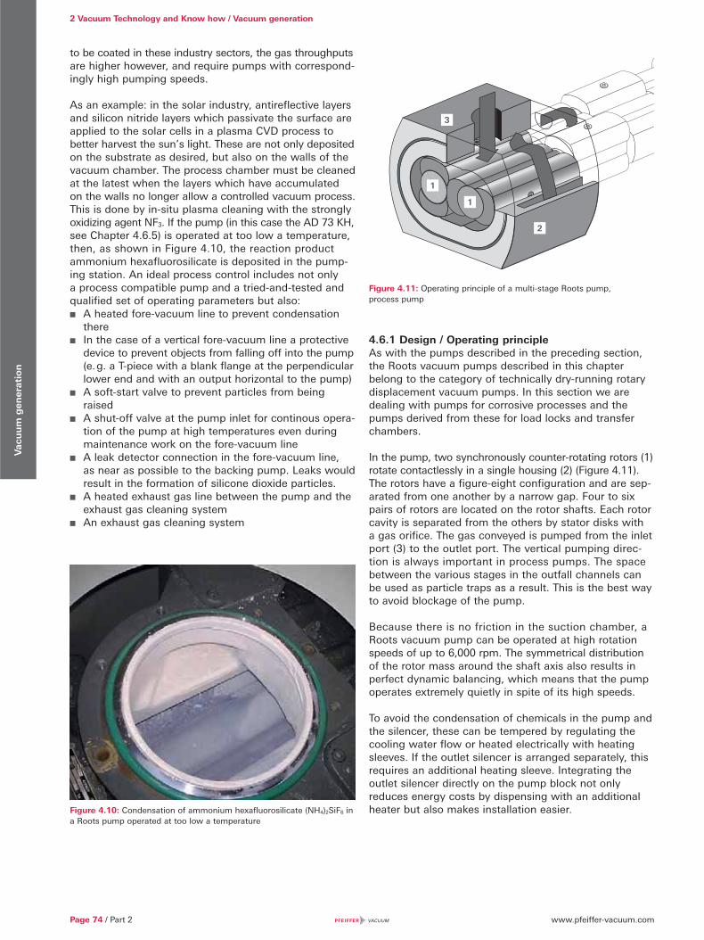
www.pfeiffer-vacuum.comPage 74 / Part 2
2 Vacuum Technology and Know how / Vacuum generationV
acu
um
gen
erat
ion
to be coated in these industry sectors, the gas throughputs are higher however, and require pumps with correspond-ingly high pumping speeds.
As an example: in the solar industry, antireflective layers and silicon nitride layers which passivate the surface are applied to the solar cells in a plasma CVD process to better harvest the sun’s light. These are not only deposited on the substrate as desired, but also on the walls of the vacuum chamber. The process chamber must be cleaned at the latest when the layers which have accumulated on the walls no longer allow a controlled vacuum process. This is done by in-situ plasma cleaning with the strongly oxidizing agent NF3. If the pump (in this case the AD 73 KH, see Chapter 4.6.5) is operated at too low a temperature, then, as shown in Figure 4.10, the reaction product ammonium hexafluorosilicate is deposited in the pump-ing station. An ideal process control includes not only a process compatible pump and a tried-and-tested and qualified set of operating parameters but also:
A heated fore-vacuum line to prevent condensation there
In the case of a vertical fore-vacuum line a protective device to prevent objects from falling off into the pump (e. g. a T-piece with a blank flange at the perpendicular lower end and with an output horizontal to the pump)
A soft-start valve to prevent particles from being raised
A shut-off valve at the pump inlet for continous opera-tion of the pump at high temperatures even during maintenance work on the fore-vacuum line
A leak detector connection in the fore-vacuum line, as near as possible to the backing pump. Leaks would result in the formation of silicone dioxide particles.
A heated exhaust gas line between the pump and the exhaust gas cleaning system
An exhaust gas cleaning system
Figure 4.10: Condensation of ammonium hexafluorosilicate (NH4)2SiF6 in a Roots pump operated at too low a temperature
4.6.1 Design / Operating principleAs with the pumps described in the preceding section, the Roots vacuum pumps described in this chapter belong to the category of technically dry-running rotary displacement vacuum pumps. In this section we are dealing with pumps for corrosive processes and the pumps derived from these for load locks and transfer chambers.
In the pump, two synchronously counter-rotating rotors (1) rotate contactlessly in a single housing (2) (Figure 4.11). The rotors have a figure-eight configuration and are sep-arated from one another by a narrow gap. Four to six pairs of rotors are located on the rotor shafts. Each rotor cavity is separated from the others by stator disks with a gas orifice. The gas conveyed is pumped from the inlet port (3) to the outlet port. The vertical pumping direc-tion is always important in process pumps. The space between the various stages in the outfall channels can be used as particle traps as a result. This is the best way to avoid blockage of the pump.
Because there is no friction in the suction chamber, a Roots vacuum pump can be operated at high rotation speeds of up to 6,000 rpm. The symmetrical distribution of the rotor mass around the shaft axis also results in perfect dynamic balancing, which means that the pump operates extremely quietly in spite of its high speeds.
To avoid the condensation of chemicals in the pump and the silencer, these can be tempered by regulating the cooling water flow or heated electrically with heating sleeves. If the outlet silencer is arranged separately, this requires an additional heating sleeve. Integrating the outlet silencer directly on the pump block not only reduces energy costs by dispensing with an additional heater but also makes installation easier.
Figure 4.11: Operating principle of a multi-stage Roots pump, process pump
1
1
2
3

www.pfeiffer-vacuum.com
2 Vacuum Technology and Know how / Vacuum generation
Part 2 / Page 75
Vac
uu
m g
ener
atio
n
4.6.2 ApplicationAdvantages of multi-stage Roots pumps in a corrosive gas version include:
Ideal adjustment to the vacuum process concerned by adjusting the temperature, the purge gas throughput and the rotation speed.
No lubricant in the gas displacement area No operating fluid disposal problems High reliability and system uptime Long service intervals, low power consumption and
media consumption of cooling water and flushing gas, and low cost of ownership as a result
Small footprint, with good integration and savings in cleanrooms and pump levels
Extensive controlling options, local or remote control, integration in a monitoring network
Minimal leak rate Ideal backing pump for turbopumps and Roots pumps
in corrosive processes Certified to UL/CSA and SEMI S2
Dust and particlesProcess pumps are exposed to particles that are conveyed to the pump from process chambers and fore-vacuum lines. In addition, particles and deposits that may result from the condensation of reaction byproducts in the pumps themselves must also be tolerated. Ideally, it is possible to avoid the formation of particles and deposits by using adjustable heating and controlled temperature patterns. By pumping in a vertical direction, any particles drop out of the pump stage and remain in the outfall channel to the next stage. After the next ventilation and the subsequent pumpdown, the particles will be dis-charged by the displaced gas into the next stage that follows. This discharging mechanism expels more than 98 % of the particles generated from the inlet to the outlet. This means that a central exhaust gas cleaning system which captures and disposes of not just process chemi-cals but also particles can be provided at the pump outlet. High-maintenance traps and filters on the intake side can be avoided wherever possible in vacuum solutions for corrosive, toxic and condensable media.
Corrosive gasesMulti-stage Roots pumps of the P and H series are specially designed for corrosive gas processes in the semiconductor, solar and coating industry for flat screens. Both the metal rotors and stators as well as the elastomer materials of the pumps are made of highly corrosion-resistant materials.
Leakage rateThe high tightness and the protection from gases diffusing back from the ambient air or an exhaust gas cleaning system or scrubber through a non-return valve make multi-stage Roots pumps the perfect solution for corrosive gas applications. Encapsulated motors are also part of the anti-leak concept.
4.6.3 Load locks and noncorrosive gasesThe ACP 120 is an entry-level model of water cooled multi-stage Roots pumps. Pumps in the ACP series are not suitable for pumping down large quantities of corrosive gases. However, ACP series pumps can be used to handle at least traces of corrosive gases. In this case, inert gas purge is used in which the bearings are protected with an inert gas curtain and process gases are diluted by introducing inert gas into the pump stages.
The ACP 120 can either be operated as a stand-alone pump or in combination with a Roots pump as an ACG 600 pumping station that is an ideal solution for industrial use and which benefits from the design of corrosive gas versions for the semiconductor industry. ACP/ACG pumps are ideally suited for clean processes through their friction-free design. They achieve excellent long-term stability and long maintenance intervals.
Figure 4.12: ACP 120
Lock pumps for the semiconductor industry have an ”L“ for ”load lock“ in their designation. In contrast to the ACP 120 described above, they are equipped with a housing and a controller. A frequency converter ensures globally reproducible performance parameters irrespective of the mains voltage and frequency.
L-series pumps are fitted with an operating hour counter, status lights and a and can be operated in a local and remote control mode between local and remote control mode.
Inlet and outlet flanges are fitted to the rear of the pump as well as an input-output interface which allows it to be linked to the control unit of a semiconductor produc-tion machine. A serial interface is optionally available to enable the pump, for example, to be connected to a monitoring network. Connections for water cooling and an optional energy-saving option are also located on the rear of the pumps (see Figure 4.13).
The optional energy-saving option (Energy Saving, ES) integrated in the pump housing reduces the pump power consumption by up to 50 %. The cost of ownership for the operator is significantly reduced as a result. Besides saving energy, the A 100 L ES can attain an ultimate pressure of 7 · 10-4 hPa. The noise level is also reduced by 3 dB(A).

www.pfeiffer-vacuum.comPage 76 / Part 2
2 Vacuum Technology and Know how / Vacuum generationV
acu
um
gen
erat
ion
By keeping the pump surfaces free, the units can also be stacked and therefore minimize the space taken in the cleanroom of a semiconductor fab or in a the basement. Thanks to its combination of a minimal footprint, stack-ability, high pumping speed even at atmospheric pres-sure, energy-saving option, low ultimate pressure and high reliability and long-term stability, the L series is the ideal solution for all load-lock processes.
The low final pressure and the reduced noise level make them attractive for analytical and research and develop-ment applications.
4.6.4 Process chemistryIn coating process, specially in the production of semi-conductors, flat screens and in the solar industry, as demonstrated in the introduction to this chapter, the corrosion resistance of vacuum pumps is of great significance. Besides the process compatibility, the small footprint and the low operating costs are particularly important pump parameters. The P series meets these requirements by lowering power input up to 53 % compared to the previous model while maintaining the same footprint.
This pump series is based on the A 103 P dry-running process pump. We have taken two models from the series and supplemented them with Roots pumps for enhanced pumping speeds and gas throughput in the process pressure range. The power input is kept low due to the six-stage design of the A 103 P and an energy-efficient motor. The six-stage design of the A 103 P reduces the differential pressures between the various stages and also the power input of the pump. Besides the sixth stage, the large-dimensioned inlet stage and the high rotation speed allow for a high pumping speed and a low ultimate pressure.
Placing the silencer on the outlet side directly on the pump block makes for a compact pump design and energy savings through direct heating of the silencer by the pump block without the need for an additional heating sleeve. Temperature-controlled and continuously monitored heating of the entire pump is necessary to prevent the condensation of reaction byproducts.
Due to the P series standby option, not only does the pump use less cooling water, but it also reduces flushing
gas consumption beyond the process operation which results in the reduction of operating costs.
Extensive activating and controlling options allow not only a manual control mode but also control through a system control and connection to a monitoring network. Important parameters can be outputted directly and exported for statistical evaluation.
The P series is CE and SEMI S2 compliant.
4.6.5 Harsh process chemistryThe ongoing development of processes especially in the semiconductor and solar industry places constantly new demands on the vacuum pumps used. Based on the proven technology of multi-stage Roots pumps, Pfeiffer Vacuum provides the perfect solution for demanding processes in these industry sectors with its H series. The gas throughput at the process pressure, the particle tolerance and the resistance to condensation have been significantly increased in comparison with previous pump solutions.
As with the P (for Process) series pumps, H series (for Harsh Process) pumps are equipped with a temperature control and an inert gas flushing system. The parameter range for optimizing adjustment to the process is far wider, however, than in pumps in the P series.
This pump series is based on the A 203 H dry-running process pump. We have taken three additional models from the series and supplemented them with Roots pumps for enhanced pumping speeds and gas through-put in the process pressure range. Due to the use of specific materials, the corrosive gas equipment of these pumps also makes it possible to use strong oxidizing agents such as NF3. The broad temperature range of the pumps enables them to adapt to widely differing processes such as tungsten deposition at low tempera-tures or nitride deposition at high temperatures. A highly efficient motor results in energy savings at low pressures and provides good startup properties after pump downtime due to its high torque.
The models in the A3H series are ideally compatible with pumps in the P series thanks to their identical interfaces and identical media connections. This means that if a process is changed on an existing production
Figure 4.13: A 100 L rear side with connections Figure 4.14: A 203 H cross-section
DN 50 KF inletMains power connection
Water ¼ NPT QCs
CDA 1/8" Swagelock(intake side option)
DN 25 KF outletRS232/485 interface(option)
SPI interface16 or 19 pins

www.pfeiffer-vacuum.com
2 Vacuum Technology and Know how / Vacuum generation
Part 2 / Page 77
Vac
uu
m g
ener
atio
n
plant, optimized pump solutions can be obtained with a minimum of installation work by exchanging the pumps.
Supplementing the A 1803 H model with a third Roots stage provides a compact and extremely powerful pumping station with maximum pumping speeds for CVD processes. The AD 73 KH uses a frequency- controlled Roots pump with a rated pumping speed of 4,500 m³ · h-1 in its own frame over the dry-running process pump. Installation is easy due to the modular
structure and the various pumps in the pumping station can be taken out singly and maintained in the event of servicing work. The frequency converter of the Roots pump on the intake side allows adjustment to the pro-cess parameters over a broad gas throughput range and for widely differing process gases.
Pfeiffer Vacuum monitors the dynamic development of processes in the various sectors of industry on an ongoing basis and will continue in the future to deliver optimized pump solutions to meet these requirements. An initial overview is given in Chapter 8, Contamination Management Solutions.
4.6.6 Portfolio overview
4.6.6.1 Water cooled process pumpsThe pumping speed and final pressure of the ACP 120 / ACP 120 G can be increased further increased by combining them with a Roots pumps. Optimized pump versions are available for larger volumes.
The technical data provided are given for a mains frequency of 50 Hz. Standard not more than 1 m3. Special versions of A 203 H and A 1803 H type pumps are suitable for volumes of up to 50 m3.
Figure 4.15: A 1503 H process pumping station
Multi-stage Roots pumps for noncorrosive applications
Model Pumping speed Ultimate pressure with/without purge gas
Applications
ACP 120 95 m³ · h-1 3 · 10-2 hPa Load locks and transfer chambers with a volume of up to 1 m3, noncorrosive gases, noble gases, regeneration of cryo pumps, backing pumps for turbopumps with noncorrosive gases
ACP 120 G 95 m³ · h-1 9 · 10-2 hPa with 35 slm purge gas
A 100 L 100 m³ · h-1 6.6 · 10-3 hPa
A 100 L ES 100 m³ · h-1 7 · 10-4 hPa
Table 4.16: Performance data for water cooled multi-stage Roots pumps for noncorrosive applications
Multi-stage Roots pumps for corrosive applications
Model Pumping speed Ultimate pressure with/without purge gas
Applications
A 103 P 120 m³ · h-1 6.5 · 10-3 hPa2.6 · 10-2 hPa with 20 slm purge gas Dry etching (oxide and poly)
AshingStrippingRTPImplantation
A 603 P 480 m³ · h-1 5 · 10-4 hPa2 · 10-3 hPa with 20 slm purge gas
A 1003 P 900 m³ · h-1 3 · 10-4 hPa1 · 10-3 hPa with 20 slm purge gas
Table 4.17: Performance data for P series water cooled multi-stage Roots pumps for corrosive applications
Multi-stage Roots pumps for corrosive applications (harsh processes)
Model Pumping speedUltimate pressure without/with purge gas
Applications
A 203 H 130 m³ · h-1 6 · 10-2 hPa5 · 10-1 hPa with 50 slm purge gas
Metal etchingCVD (PECVD, SACVD, LPCVD)ALDEpitaxyDry etching
A 803 H 600 m³ · h-1 1 · 10-3 hPa1 · 10-2 hPa with 50 slm purge gas
A 1503 H 1,100 m³ · h-1 2 · 10-3 hPa9 · 10-3 hPa with 50 slm purge gas
A 1803 H 1,650 m³ · h-1 2 · 10-3 hPa9 · 10-3 hPa with 50 slm purge gas
AD 73 KH 4,700 m³ · h-1 8 · 10-4 hPa3 · 10-3 hPa with 50 slm purge gas
Table 4.18: Performance data for H series water cooled multi-stage Roots pumps for corrosive applications (harsh processes)
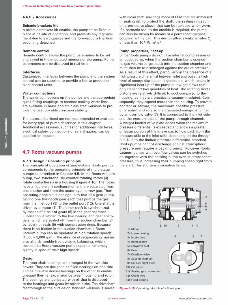
www.pfeiffer-vacuum.comPage 78 / Part 2
2 Vacuum Technology and Know how / Vacuum generationV
acu
um
gen
erat
ion
4.6.6.2 Accessories
Seismic brackets kitA seismic brackets kit enables the pump to be fixed in place at its site of operation, and prevents any displace-ment due to earthquakes and the fore-vacuum line from becoming detached.
Remote controlRemote control allows the pump parameters to be set and saved in the integrated memory of the pump. Pump parameters can be displayed in real time.
InterfacesCustomized interfaces between the pump and the system control can be supplied to provide a link to production plant control units.
Water connectionsThe water connections on the pumps and the appropriate quick fitting couplings to connect cooling water lines are available in brass and stainless steel versions to pro-vide the best possible corrosion stability.
The accessories listed are not recommended or available for every type of pump described in this chapter. Additional accessories, such as for additional interfaces, electrical safety, connections or safe shipping, can be supplied on request.
4.7 Roots vacuum pumps
4.7.1 Design / Operating principleThe principle of operation of single-stage Roots pumps corresponds to the operating principle of multi-stage pumps as described in Chapter 4.5. In the Roots vacuum pump, two synchronously counter-rotating rotors (4) rotate contactlessly in a housing (Figure 4.16). The rotors have a figure-eight configuration and are separated from one another and from the stator by a narrow gap. Their operating principle is analogous to that of a gear pump having one two-tooth gear each that pumps the gas from the inlet port (3) to the outlet port (12). One shaft is driven by a motor (1). The other shaft is synchronized by means of a pair of gears (6) in the gear chamber. Lubrication is limited to the two bearing and gear cham-bers, which are sealed off from the suction chamber (8) by labyrinth seals (5) with compression rings. Because there is no friction in the suction chamber, a Roots vacuum pump can be operated at high rotation speeds (1,500 – 3,000 rpm ). The absence of reciprocating masses also affords trouble-free dynamic balancing, which means that Roots vacuum pumps operate extremely quietly in spite of their high speeds.
DesignThe rotor shaft bearings are arranged in the two side covers. They are designed as fixed bearings on one side and as movable (loose) bearings on the other to enable unequal thermal expansion between housing and rotor. The bearings are lubricated with oil that is displaced to the bearings and gears by splash disks. The driveshaft feedthrough to the outside on standard versions is sealed
with radial shaft seal rings made of FPM that are immersed in sealing oil. To protect the shaft, the sealing rings run on a protective sleeve that can be replaced when worn. If a hermetic seal to the outside is required, the pump can also be driven by means of a permanent-magnet coupling with a can. This design affords leakage rates QI of less than 10-6 Pa m3 s-1.
Pump properties, heat-upSince Roots pumps do not have internal compression or an outlet valve, when the suction chamber is opened its gas volume surges back into the suction chamber and must then be re-discharged against the outlet pressure. As a result of this effect, particularly in the presence of a high pressure differential between inlet and outlet, a high level of energy dissipation is generated, which results in significant heat-up of the pump at low gas flows that only transport low quantities of heat. The rotating Roots pistons are relatively difficult to cool compared to the housing, as they are practically vacuum-insulated. Con-sequently, they expand more than the housing. To prevent contact or seizure, the maximum possible pressure differential, and so also the dissipated energy, is limited by an overflow valve (7). It is connected to the inlet side and the pressure side of the pump-through channels. A weight-loaded valve plate opens when the maximum pressure differential is exceeded and allows a greater or lesser portion of the intake gas to flow back from the pressure side to the inlet side, depending on the through-put. Due to the limited pressure differential, standard Roots pumps cannot discharge against atmospheric pressure and require a backing pump. However Roots vacuum pumps with overflow valves can be switched on together with the backing pump even at atmospheric pressure, thus increasing their pumping speed right from the start. This shortens evacuation times.
Figure 4.16: Operating principle of a Roots pump
4 8 7
13 10 12 11 10
965
2
3
1
1) Motor
2) Loose bearing
3) Intake port
4) Roots piston
5) Labyrinth seal
6) Gear
7) Overflow valve
8) Suction chamber
9) Oil level sight glass
10) Oil return
11) Sealing gas connection
12) Outlet port
13) Fixed bearing
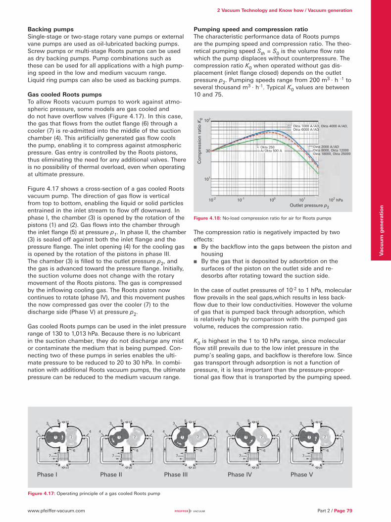
www.pfeiffer-vacuum.com
2 Vacuum Technology and Know how / Vacuum generation
Part 2 / Page 79
Vac
uu
m g
ener
atio
n
Backing pumpsSingle-stage or two-stage rotary vane pumps or external vane pumps are used as oil-lubricated backing pumps. Screw pumps or multi-stage Roots pumps can be used as dry backing pumps. Pump combinations such as these can be used for all applications with a high pump-ing speed in the low and medium vacuum range. Liquid ring pumps can also be used as backing pumps.
Gas cooled Roots pumpsTo allow Roots vacuum pumps to work against atmo-spheric pressure, some models are gas cooled and do not have overflow valves (Figure 4.17). In this case, the gas that flows from the outlet flange (6) through a cooler (7) is re-admitted into the middle of the suction chamber (4). This artificially generated gas flow cools the pump, enabling it to compress against atmospheric pressure. Gas entry is controlled by the Roots pistons, thus eliminating the need for any additional valves. There is no possibility of thermal overload, even when operating at ultimate pressure.
Figure 4.17 shows a cross-section of a gas cooled Roots vacuum pump. The direction of gas flow is vertical from top to bottom, enabling the liquid or solid particles entrained in the inlet stream to flow off downward. In phase I, the chamber (3) is opened by the rotation of the pistons (1) and (2). Gas flows into the chamber through the inlet flange (5) at pressure p1. In phase II, the chamber (3) is sealed off against both the inlet flange and the pressure flange. The inlet opening (4) for the cooling gas is opened by the rotation of the pistons in phase III. The chamber (3) is filled to the outlet pressure p2, and the gas is advanced toward the pressure flange. Initially, the suction volume does not change with the rotary movement of the Roots pistons. The gas is compressed by the inflowing cooling gas. The Roots piston now continues to rotate (phase IV), and this movement pushes the now compressed gas over the cooler (7) to the discharge side (Phase V) at pressure p2.
Gas cooled Roots pumps can be used in the inlet pressure range of 130 to 1,013 hPa. Because there is no lubricant in the suction chamber, they do not discharge any mist or contaminate the medium that is being pumped. Con-necting two of these pumps in series enables the ulti-mate pressure to be reduced to 20 to 30 hPa. In combi-nation with additional Roots vacuum pumps, the ultimate pressure can be reduced to the medium vacuum range.
Pumping speed and compression ratioThe characteristic performance data of Roots pumps are the pumping speed and compression ratio. The theo-retical pumping speed Sth = S0 is the volume flow rate which the pump displaces without counterpressure. The compression ratio K0 when operated without gas dis-placement (inlet flange closed) depends on the outlet pressure p2. Pumping speeds range from 200 m3 · h -1 to several thousand m3 · h-1. Typical K0 values are between 10 and 75.
Figure 4.18: No-load compression ratio for air for Roots pumps
The compression ratio is negatively impacted by two effects:
By the backflow into the gaps between the piston and housing
By the gas that is deposited by adsorbtion on the surfaces of the piston on the outlet side and re-desorbs after rotating toward the suction side.
In the case of outlet pressures of 10-2 to 1 hPa, molecular flow prevails in the seal gaps,which results in less back-flow due to their low conductivities. However the volume of gas that is pumped back through adsorption, which is relatively high by comparison with the pumped gas volume, reduces the compression ratio.
K0 is highest in the 1 to 10 hPa range, since molecular flow still prevails due to the low inlet pressure in the pump’s sealing gaps, and backflow is therefore low. Since gas transport through adsorption is not a function of pressure, it is less important than the pressure-propor-tional gas flow that is transported by the pumping speed.
Figure 4.17: Operating principle of a gas cooled Roots pump
Phase I Phase II Phase III Phase IV Phase V
21 21 21 21 21
4
35
4
6
7
p1
p2
4
35
4
6
7
p1
p2
4
35
4
6
7
p1
p2
4
35
4
6
7
p1
p2
4
35
4
6
7
p1
p2
Okta 2000 A / ADOkta 8000, Okta 12000Okta 18000, Okta 25000
Okta 250 A / Okta 500 A
Outlet pressure p2
10-2 10-1 100 101 102 hPa
102
30
101
Co
mp
ress
ion
rat
io K
0
Okta 1000 A / AD, Okta 4000 A / AD, Okta 6000 A / AD
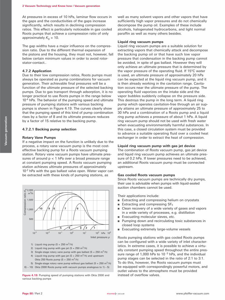
www.pfeiffer-vacuum.comPage 80 / Part 2
2 Vacuum Technology and Know how / Vacuum generationV
acu
um
gen
erat
ion
At pressures in excess of 10 hPa, laminar flow occurs in the gaps and the conductivities of the gaps increase significantly, which results in declining compression ratios. This effect is particularly noticeable in gas cooled Roots pumps that achieve a compression ratio of only approximately K0 = 10.
The gap widths have a major influence on the compres-sion ratio. Due to the different thermal expansion of the pistons and the housing, they must not, however, fall below certain minimum values in order to avoid rotor-stator-contact..
4.7.2 ApplicationDue to their low compression ratios, Roots pumps must always be operated as pump combinations for vacuum generation. Their achievable final pressures will be a function of the ultimate pressure of the selected backing pumps. Due to gas transport through adsorption, it is no longer practical to use Roots pumps in the range below 10-4 hPa. The behavior of the pumping speed and ultimate pressure of pumping stations with various backing pumps is shown in Figure 4.19. The curves clearly show that the pumping speed of this kind of pump combination rises by a factor of 8 and its ultimate pressure reduces by a factor of 15 relative to the backing pump.
4.7.2.1 Backing pump selection
Rotary Vane PumpsIf a negative impact on the function is unlikely due to the process, a rotary vane vacuum pump is the most cost-effective backing pump for a Roots vacuum pumping station. Rotary vane vacuum pumps have ultimate pres-sures of around p < 1 hPa over a broad pressure range at constant pumping speed. A Roots vacuum pumping station achieves ultimate pressures of approximately 10-2 hPa with the gas ballast valve open. Water vapor can be extracted with these kinds of pumping stations, as
well as many solvent vapors and other vapors that have sufficiently high vapor pressures and do not chemically decompose the pump oil. Examples of these include alcohols, halogenated hydrocarbons, and light normal paraffin as well as many others besides.
Liquid ring vacuum pumpsLiquid ring vacuum pumps are a suitable solution for extracting vapors that chemically attack and decompose the backing pump oil or that have such low vapor pressure that condensation in the backing pump cannot be avoided, in spite of gas ballast. However they will only achieve an ultimate pressure that is determined by the vapor pressure of the operating fluid. If 15°C water is used, an ultimate pressure of approximately 20 hPa can be expected at the liquid ring vacuum pump, and it is then already working in the cavitation range. Cavita-tion occurs near the ultimate pressure of the pump. The operating fluid vaporizes on the intake side and the vapor bubbles suddenly collapse on the pressure side. This destroys the pump in the long term. A liquid ring pump which operates cavitation-free through an air sup-ply attains an ultimate pressure of approximately 25 to 30 hPa and a combination of a Roots pump and a liquid ring pump achieves a presssure of about 1 hPa. A liquid ring vacuum pump should not be used with fresh water when evacuating environmentally harmful substances. In this case, a closed circulation system must be provided to advance a suitable operating fluid over a cooled heat exchanger in order to extract the heat of compression.
Liquid ring vacuum pump with gas jet deviceThe combination of Roots vacuum pump, gas jet device and liquid ring vacuum pump achieves an ultimate pres-sure of 0.2 hPa. If lower pressures need to be achieved, an additional Roots vacuum pump must be connected upstream.
Gas cooled Roots vacuum pumpsSince Roots vacuum pumps are technically dry pumps, their use is advisable when pumps with liquid-sealed suction chambers cannot be used.
Their applications include: Extracting and compressing helium on cryostats Extracting and compressing SF6
Clean recovery of a wide variety of gases and vapors in a wide variety of processes, e.g. distillation
Evacuating molecular sieves, etc. Pumping down and recirculating toxic substances in
closed loop systems Evacuating extremely large-volume vessels
Roots pumping stations with gas cooled Roots pumps can be configured with a wide variety of inlet character-istics. In extreme cases, it is possible to achieve a virtu-ally constant pumping speed throughout the entire pres-sure range of 1,000 hPa to 10 -3 hPa, and the individual pump stages can be selected in the ratio of 2:1 to 3:1. To do this, however, the Roots vacuum pumps must be equipped with correspondingly powerful motors, and outlet valves to the atmosphere must be provided instead of overflow valves. Figure 4.19: Pumping speed of pumping stations with Okta 2000 and
various backing pumps
1) Liquid ring pump (S = 250 m3 / h)
2) Liquid ring pump with gas jet (S = 250 m3 / h)
3) Single-stage rotary vane pump with gas ballast (S = 250 m3 / h)
4) Liquid ring pump with gas jet (S = 250 m3 / h) and upstream
Okta 250 Roots pump (S = 250 m3 / h)
5) Single-stage rotary vane pump without gas ballast (S = 250 m3 / h)
6) – 10) Okta 2000 Roots pump with vacuum pumps analogous to 1) – 5)
2,000m3/h
1,500
1,000
500
Co
mp
ress
ion
rat
io K
0
Inlet pressure p
10-3 10-2 10-1 100 101 102 hPa 103
12345
678910
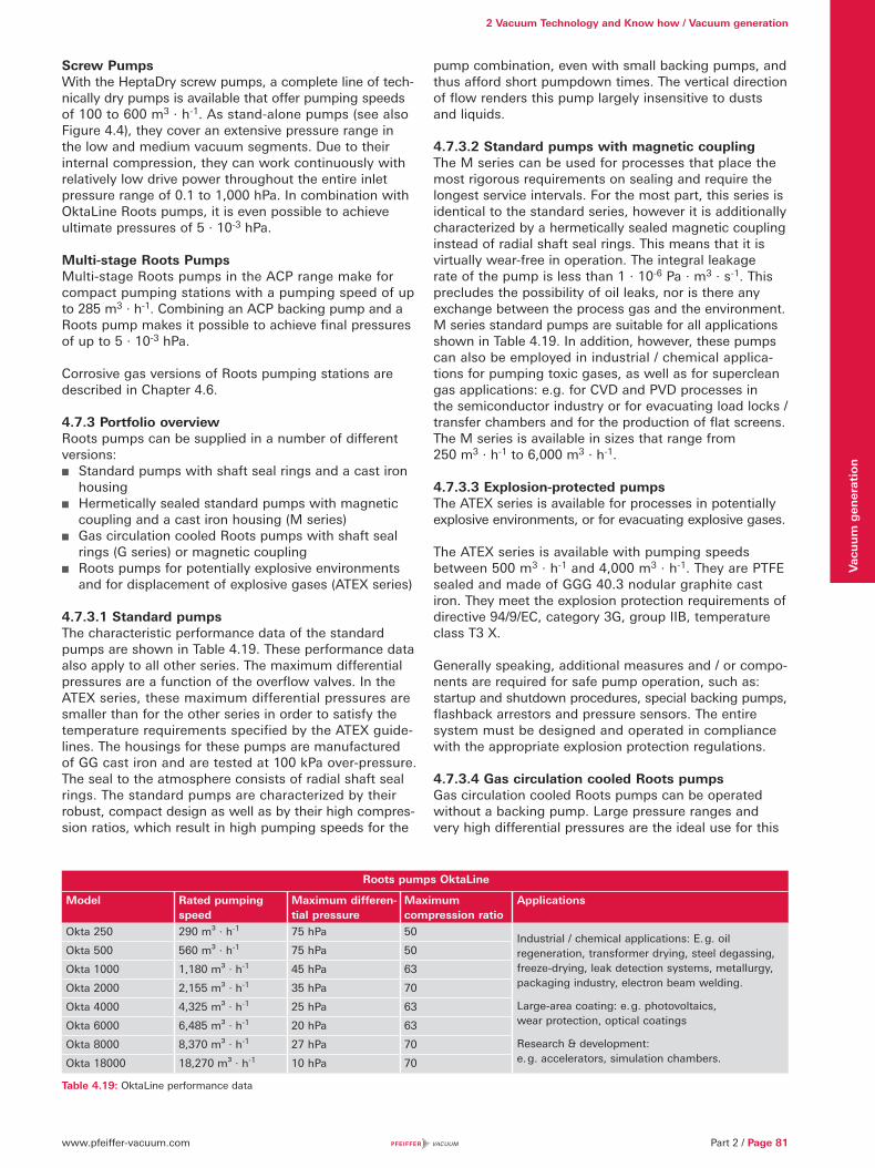
www.pfeiffer-vacuum.com
2 Vacuum Technology and Know how / Vacuum generation
Part 2 / Page 81
Vac
uu
m g
ener
atio
n
Screw PumpsWith the HeptaDry screw pumps, a complete line of tech-nically dry pumps is available that offer pumping speeds of 100 to 600 m3 · h-1. As stand-alone pumps (see also Figure 4.4), they cover an extensive pressure range in the low and medium vacuum segments. Due to their internal compression, they can work continuously with relatively low drive power throughout the entire inlet pressure range of 0.1 to 1,000 hPa. In combination with OktaLine Roots pumps, it is even possible to achieve ultimate pressures of 5 · 10-3 hPa.
Multi-stage Roots PumpsMulti-stage Roots pumps in the ACP range make for compact pumping stations with a pumping speed of up to 285 m3 · h-1. Combining an ACP backing pump and a Roots pump makes it possible to achieve final pressures of up to 5 · 10-3 hPa.
Corrosive gas versions of Roots pumping stations are described in Chapter 4.6.
4.7.3 Portfolio overviewRoots pumps can be supplied in a number of different versions:
Standard pumps with shaft seal rings and a cast iron housing
Hermetically sealed standard pumps with magnetic coupling and a cast iron housing (M series)
Gas circulation cooled Roots pumps with shaft seal rings (G series) or magnetic coupling
Roots pumps for potentially explosive environments and for displacement of explosive gases (ATEX series)
4.7.3.1 Standard pumpsThe characteristic performance data of the standard pumps are shown in Table 4.19. These performance data also apply to all other series. The maximum differential pressures are a function of the overflow valves. In the ATEX series, these maximum differential pressures are smaller than for the other series in order to satisfy the temperature requirements specified by the ATEX guide-lines. The housings for these pumps are manufactured of GG cast iron and are tested at 100 kPa over-pressure. The seal to the atmosphere consists of radial shaft seal rings. The standard pumps are characterized by their robust, compact design as well as by their high compres-sion ratios, which result in high pumping speeds for the
pump combination, even with small backing pumps, and thus afford short pumpdown times. The vertical direction of flow renders this pump largely insensitive to dusts and liquids.
4.7.3.2 Standard pumps with magnetic couplingThe M series can be used for processes that place the most rigorous requirements on sealing and require the longest service intervals. For the most part, this series is identical to the standard series, however it is additionally characterized by a hermetically sealed magnetic coupling instead of radial shaft seal rings. This means that it is virtually wear-free in operation. The integral leakage rate of the pump is less than 1 · 10-6 Pa · m3 · s-1. This precludes the possibility of oil leaks, nor is there any exchange between the process gas and the environment. M series standard pumps are suitable for all applications shown in Table 4.19. In addition, however, these pumps can also be employed in industrial / chemical applica-tions for pumping toxic gases, as well as for superclean gas applications: e.g. for CVD and PVD processes in the semiconductor industry or for evacuating load locks / transfer chambers and for the production of flat screens. The M series is available in sizes that range from 250 m3 · h-1 to 6,000 m3 · h-1.
4.7.3.3 Explosion-protected pumpsThe ATEX series is available for processes in potentially explosive environments, or for evacuating explosive gases.
The ATEX series is available with pumping speeds between 500 m3 · h-1 and 4,000 m3 · h-1. They are PTFE sealed and made of GGG 40.3 nodular graphite cast iron. They meet the explosion protection requirements of directive 94/9/EC, category 3G, group IIB, temperature class T3 X.
Generally speaking, additional measures and / or compo-nents are required for safe pump operation, such as: startup and shutdown procedures, special backing pumps, flashback arrestors and pressure sensors. The entire system must be designed and operated in compliance with the appropriate explosion protection regulations.
4.7.3.4 Gas circulation cooled Roots pumpsGas circulation cooled Roots pumps can be operated without a backing pump. Large pressure ranges and very high differential pressures are the ideal use for this
Roots pumps OktaLine
Model Rated pumping speed
Maximum differen-tial pressure
Maximum compression ratio
Applications
Okta 250 290 m³ · h-1 75 hPa 50Industrial / chemical applications: E. g. oil regeneration, transformer drying, steel degassing, freeze-drying, leak detection systems, metallurgy, packaging industry, electron beam welding.
Large-area coating: e. g. photovoltaics, wear protection, optical coatings
Research & development: e. g. accelerators, simulation chambers.
Okta 500 560 m³ · h-1 75 hPa 50
Okta 1000 1,180 m³ · h-1 45 hPa 63
Okta 2000 2,155 m³ · h-1 35 hPa 70
Okta 4000 4,325 m³ · h-1 25 hPa 63
Okta 6000 6,485 m³ · h-1 20 hPa 63
Okta 8000 8,370 m³ · h-1 27 hPa 70
Okta 18000 18,270 m³ · h-1 10 hPa 70
Table 4.19: OktaLine performance data

www.pfeiffer-vacuum.comPage 82 / Part 2
2 Vacuum Technology and Know how / Vacuum generationV
acu
um
gen
erat
ion
type of pump. Continuous use is possible at high differ-ential pressures since the gas that is heated up by compression is cooled on the pressure side and partly fed back into the suction chamber. This makes them suitable for operation at atmospheric pressure if they are used in combination with gas coolers. Gas circulation cooled Roots pumps are available in sizes from 500 m3 · h-1 (18.5 kW drive power) up to 8,000 m3 · h-1 (200 kW drive power).
4.7.4 AccessoriesSplinter shield inserts are offered as accessories for all OktaLine series Roots pumps.
The following oils for lubricating the gearing and the bearings are available as lubricants (Table 4.11):
Mineral oil P3 (in 0.5 l to 200 l containers) Perfluoropolyether F5 (in 0.5 l to 50 l containers) Diester oil D1 (in 0.5 l to 200 l containers)
Caution: Different kinds of oil should not be mixed. The pumps are prepared at delivery for one of these types of oil.
Since many Roots pumps are installed in pump combina-tions, it is possible to integrate the following accessories on an as-needed basis:
Electrical controllers Measuring instrumentation for temperature and
pressure Pressure regulation systems Heat exchangers and condensers Soundproofing encapsulation for indoor and outdoor
installation Silencers Dust separators Flushing devices Vibration isolation Liquid separators Gear chamber evacuation Sealing gas supply
Measurement connectionsIn the case of many Roots pumps, it is possible to use the measurement connections on the inlet and pressure sides of the pump. To do this, the existing locking screws can be replaced with small ISO KF flange unions. This enables appropriate temperature sensors and pressure sensors to be connected for monitoring the pump.
Sealing gas connectionWhen pumping solvents or reactive gases, the risk exists that the lubricant will be significantly diluted as a result of condensation. Reactive gases or vapors can also attack parts of the gear chamber. For the most part, this risk can be avoided by admitting a sealing gas in the area of the shaft feedthrough between working space and gear chamber. Inert gases, mostly nitrogen (N2), are used as the sealing gas.
Gear chamber evacuationIn the case of all processes in which large Roots vacuum pumping stations must reach certain pressures in short cycle times (fast evacuation), it is practical to pump
down the gear chambers of a Roots pump via an oil separator, by means of a separate vacuum pump in each chamber. This prevents gas from flowing out of the gear chamber and into the suction chamber, thus enabling the desired working pressure to be reached faster. The desired working pressure will determine whether it is possible to connect the gear chamber toward the backing-vacuum side of the Roots pump.
Flushing devicesA flushing device can be used for processes in which deposits form in the suction chambers. The design of this device will be coordinated individually with the customer on the basis of the specific requirements. The flushing device for standard pumps requires the use of sealing gas to prevent the flushing liquid from reaching the bearings or gear chambers.
Surface protectionIf the media to be pumped down are corrosive, compo-nents that come into contact with the product can be provided with durable surface protection. The plasma-polymer thin-layer system consists of a bonding agent layer, a corrosion-protection layer and a non-stick coating. The thickness of the layer is less than 1 �m. Upon request, the suction chamber can be phosphated, vented with nitrogen and vacuum sealed in order to provide short-term surface protection, e. g. for warehousing and shipment.
SealsRoots vacuum pumps come factory-equipped with O-rings made of FKM. For special applications, all pumps can be equipped with the specific O-rings or seals that are required for the respective application.
4.7.5 Pumping stationsPfeiffer Vacuum can supply standard Roots pumps with oil-lubricated single-stage and two-stage rotary vane pumps as well as with a selection of dry pumps. Please refer to Chapter 3.1, page 242, for more information.
In addition to standard pumping stations, Pfeiffer Vacuum’s vacuum system group designs and manufactures customized pumping stations (Roots pumping stations and turbo pumping stations).
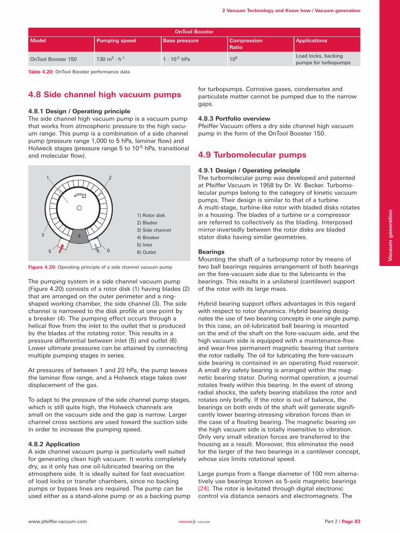
www.pfeiffer-vacuum.com
2 Vacuum Technology and Know how / Vacuum generation
Part 2 / Page 83
Vac
uu
m g
ener
atio
n
4.8 Side channel high vacuum pumps
4.8.1 Design / Operating principleThe side channel high vacuum pump is a vacuum pump that works from atmospheric pressure to the high vacu-um range. This pump is a combination of a side channel pump (pressure range 1,000 to 5 hPa, laminar flow) and Holweck stages (pressure range 5 to 10-5 hPa, transitional and molecular flow).
Figure 4.20: Operating principle of a side channel vacuum pump
The pumping system in a side channel vacuum pump (Figure 4.20) consists of a rotor disk (1) having blades (2) that are arranged on the outer perimeter and a ring-shaped working chamber, the side channel (3). The side channel is narrowed to the disk profile at one point by a breaker (4). The pumping effect occurs through a helical flow from the inlet to the outlet that is produced by the blades of the rotating rotor. This results in a pressure differential between inlet (5) and outlet (6). Lower ultimate pressures can be attained by connecting multiple pumping stages in series.
At pressures of between 1 and 20 hPa, the pump leaves the laminar flow range, and a Holweck stage takes over displacement of the gas.
To adapt to the pressure of the side channel pump stages, which is still quite high, the Holweck channels are small on the vacuum side and the gap is narrow. Larger channel cross sections are used toward the suction side in order to increase the pumping speed.
4.8.2 ApplicationA side channel vacuum pump is particularly well suited for generating clean high vacuum. It works completely dry, as it only has one oil-lubricated bearing on the atmosphere side. It is ideally suited for fast evacuation of load locks or transfer chambers, since no backing pumps or bypass lines are required. The pump can be used either as a stand-alone pump or as a backing pump
for turbopumps. Corrosive gases, condensates and particulate matter cannot be pumped due to the narrow gaps.
4.8.3 Portfolio overviewPfeiffer Vacuum offers a dry side channel high vacuum pump in the form of the OnTool Booster 150.
4.9 Turbomolecular pumps
4.9.1 Design / Operating principleThe turbomolecular pump was developed and patented at Pfeiffer Vacuum in 1958 by Dr. W. Becker. Turbomo-lecular pumps belong to the category of kinetic vacuum pumps. Their design is similar to that of a turbine. A multi-stage, turbine-like rotor with bladed disks rotates in a housing. The blades of a turbine or a compressor are referred to collectively as the blading. Interposed mirror-invertedly between the rotor disks are bladed stator disks having similar geometries.
BearingsMounting the shaft of a turbopump rotor by means of two ball bearings requires arrangement of both bearings on the fore-vacuum side due to the lubricants in the bearings. This results in a unilateral (cantilever) support of the rotor with its large mass.
Hybrid bearing support offers advantages in this regard with respect to rotor dynamics. Hybrid bearing desig-nates the use of two bearing concepts in one single pump. In this case, an oil-lubricated ball bearing is mounted on the end of the shaft on the fore-vacuum side, and the high vacuum side is equipped with a maintenance-free and wear-free permanent magnetic bearing that centers the rotor radially. The oil for lubricating the fore-vacuum side bearing is contained in an operating fluid reservoir. A small dry safety bearing is arranged within the mag-netic bearing stator. During normal operation, a journal rotates freely within this bearing. In the event of strong radial shocks, the safety bearing stabilizes the rotor and rotates only briefly. If the rotor is out of balance, the bearings on both ends of the shaft will generate signifi-cantly lower bearing-stressing vibration forces than in the case of a floating bearing. The magnetic bearing on the high vacuum side is totally insensitive to vibration. Only very small vibration forces are transferred to the housing as a result. Moreover, this eliminates the need for the larger of the two bearings in a cantilever concept, whose size limits rotational speed.
Large pumps from a flange diameter of 100 mm alterna-tively use bearings known as 5-axis magnetic bearings [24]. The rotor is levitated through digital electronic control via distance sensors and electromagnets. The
1) Rotor disk
2) Blades
3) Side channel
4) Breaker
5) Inlet
6) Outlet
1 2
65
43
OnTool Booster
Model Pumping speed Base pressure Compression Ratio
Applications
OnTool Booster 150 130 m3 · h-1 1 · 10-5 hPa 108 Load locks, backing pumps for turbopumps
Table 4.20: OnTool Booster performance data

www.pfeiffer-vacuum.comPage 84 / Part 2
2 Vacuum Technology and Know how / Vacuum generationV
acu
um
gen
erat
ion
degrees of freedom of the movement of a turborotor are continuously monitored and readjusted in real time. The absence of mechanical contact between the rotor and housing keeps the vibration generated by the pump low. The rotor revolves around its own axis of inertia. Any imbalance due to one-sided coating or erosion (such as in plasma etching) is counteracted within broad limits.
In addition to the absence of oil on the backing-vacuum side, freedom from wear and maintenance is another advantage. In the event of a power failure, the magnetic bearings are supplied with electricity through the rota-tional energy of the pump. This enables power failures to be easily bridged for several minutes. Should the power failure be of longer duration, the rotor will safely come to a stop at a very low speed through the use of an inte-grated safety bearing. During system malfunctions, the safety bearing shuts down the rotor to avoid any damage to the pump.
Motors / DrivesBrushless DC motors that afford rotational frequencies of up to 1,500 Hz (90,000 rpm) are used to drive the rotors. This enables the blade velocities that are necessary for pumping the gases.
Today, the drives are typically attached directly to the pumps. The power supply is with 24, 48 or 72 volt direct current, generated by external power supply packs or ones that are integrated in the electronic unit of the pump.
4.9.1.1 Turbomolecular pump operating principleThe pumping effect of an arrangement consisting of rotor and stator blades is based upon the transfer of impulses from the rapidly rotating blades to the gas molecules being pumped. Molecules that collide with the blades are adsorbed there and leave the blades again after a certain period of time. In this process, blade speed is added to the thermal molecular speed. To ensure that the speed component that is transferred by the blades is not lost due to collisions with other molecules, molecular flow must prevail in the pump, i. e. the mean free path must be greater than the blade spacing
Figure 4.21: Degrees of freedom of a turbo-rotor Figure 4.22: Operating principle of the turbomolecular pump
S0 = · A · v · sin � · cos � = · A · v · sin2�1
2
1
4
In the case of kinetic pumps, a counterpressure occurs when pumping gas; this causes a backflow. The pumping speed is denoted by S0. The volume flow rate decreases as pressure increases and reaches a value of 0 at the maximum compression ratio K0.
Compression ratioThe compression ratio, which is denoted K0, can be estimated according to Gaede [25]. The following applies for a visually dense blade structure (Figure 4.22):
Formula 4-8: Turbopump compression ratio
c– Mean molecule velocity [m · s-1]v Circumferential speed [m · s-1]
The geometric ratios are taken from Figure 4.22. The factor g is between 1 and 3 [26]. From the equation, it is evident that K0 increases exponentially with blade velocity v as well as with M because
(Formula 1-10)
Consequently, the compression ratio for nitrogen, for example, is significantly higher than for hydrogen.
Volume flow rate (pumping speed)Pumping speed S0 is proportional to the inlet area A and the mean circumferential velocity of the blades v, i. e. rotational speed. Taking the blade angle � into account vields:
Formula 4-9: Turbopump pumping speed
c– = 8 · R · T� · M
V c–
Area 1
Area 2
V
t
a�
b
hcos � = t– b
X Y
XY
Z3 controlled translations (X, Y, Z)
2 controlled tiltings (X, Y)
K0 = exp · ·1
sin �
1 v
g c–

www.pfeiffer-vacuum.com
2 Vacuum Technology and Know how / Vacuum generation
Part 2 / Page 85
Vac
uu
m g
ener
atio
n
Taking into account both the entry conductance of the flange
(Formula 1-24)
as well as the optimal blade angle of 45°, produces the approximate effective pumping speed S eff of a turbopump for heavy gases (molecular weight > 20) in accordance with the following formula:
Formula 4-10: Turbopump effective pumping speed
Dividing the effective pumping speed by the bladed entry surface of the uppermost disk and taking the area blocked by the blade thickness into consideration with factor df ≈ 0.9, yields the specific pumping speed of a turbopump for nitrogen, for example (curve in Figure 4.23):
Formula 4-11: Specific pumping speed
On the Y axis in Figure 4.23 the specific pumping speed is plotted in l · s-1 · cm-2 and the mean blade velocity = � · f · (Ra + Ri ) is plotted on the X axis. Moving up vertically from this point, the point of intersection with the curve shows the pump’s maximum specific pumping speed SA. Multiplying this value by the bladed surface area of the inlet disk: A = (Ra
2 - Ri2) · �, obtains the pump-
ing speed of the pump and enables it to be compared with the catalog information.
The points plotted in Figure 4.23 are determined by Pfeiffer Vacuum on the basis of the measured values of the indicated pumps. Points far above the plotted curve are physically not possible.
The pumping speeds thus determined still tell nothing about the values for light gases, e.g. for hydrogen. If a turbopump is designed for a low ultimate pressure, pump stages with various blade angles are used and the gradation is optimized for maximum pumping speeds for hydrogen. This produces pumps with sufficient com-pression ratios for both hydrogen (approximately 1,000) and nitrogen, which should be 109 due to the high partial pressure of nitrogen in the air. In the case of pure turbomolecular pumps, backing-vacuum pressures of approximately 10-2 mbar are required due to their molec-ular flow.
CEf = · Ac–
4
S0 + LEf A · v
S0 · LEf
Seff = = 4 · +1v
c–
Seff df · v
ASA = =
4 · +1vc–
Figure 4.23: Specific turbopump pumping speeds
Figure 4.25: Pumping speed as a function of inlet pressure
Figure 4.24: Pumping speed as a function of relative molecular mass
0 20 40 60 80 100 120 140
120
100
80
60
40
20
0
Relative molecular mass M
Pu
mp
ing
sp
eed
S%
Ar
N2
CH
4
He
H2
Helium
Nitrogen
Hydrogen
Inlet pressure
Pu
mp
ing
sp
eed
S
6
5
4
3
2
1
0
0 50 100 150 200 250 300 350 400 450 500 m / s
Sp
ecif
ic p
um
pin
g s
pee
d S
A
Mean blade velocity V
l / (s · cm2)
= HiPace 80
= HiPace 300
= HiPace 700
= HiPace 1500
= HiPace 2300

www.pfeiffer-vacuum.comPage 86 / Part 2
2 Vacuum Technology and Know how / Vacuum generationV
acu
um
gen
erat
ion
4.9.1.2 Holweck stage operating principleA Holweck stage (Figure 4.26) is a multi-stage Gaede type molecular pump having a helical pump channel. Due to the rotation of the rotor, gas molecules entering the pump channel receive a stimulus velocity in the direction of the channel. Backflow losses occur through gaps between the barriers that separate the Holweck channels from each other and the rotor. The gap widths must be kept small to minimize backflow. Cylindrical sleeves (1) that rotate about helical channels in the stator (2) are used as Holweck stages. Arranging stators both outside as well as inside the rotor enables two Holweck stages to be easily integrated within one and the same pump. This means that the displaced gas particles are transported outside the rotor through the stator channel and then inside the rotor through further stator channels until they are conveyed back up to the backing pump through a collecting channel. Some modern turbopumps have several of these ”pleated“ Holweck stages.
The pumping speed S0 of the Holweck stages is equal to:
Formula 4-12: Holweck stage pumping speed
Where b·h is the channel cross section and v · cos � the velocity component in the channel direction.
The compression ratio increases exponentially as a func-tion of channel length L and velocity v · cos � [4]:
Formula 4-13: Holweck stage compression ratio
The values yielded with this formula are not attained in real Holweck stages since backflow over the barrier from the neighboring channel dramatically reduces the compression ratio, and this influence is not taken into account in Formel 4-13.
To set up a turbo pumping station with diaphragm pumps with a final pressure of between 0.5 and 5 hPa, turbopumps are today equipped with Holweck stages. These kinds of pumps are termed turbo drag pumps. Since only low pumping speeds are required to generate low base pressures due to the high pre-compression of the turbopump, the displacement channels and, in par-ticular, both the channel height as well as the clearances to the rotors can be kept extremely small, thus still providing a molecular flow in the range of 1 hPa. At the same time, this increases the compression ratios for nitrogen by the required factor of 103. The shift of the compression ratio curves to higher pressure by approxi-mately two powers of ten can be seen from Figure 4.27.
Figure 4.27: Compression ratios of pure turbopumps and turbo drag pumps
Figure 4.26: Operating principle of a Holweck stage
S0 = · b · h · v · cos �1
2
K0 = with 1< g < 3v · cos � · Lc– · g · h
1) Rotor
2) Stator with threads
2
1
� b h
1012
10 11
1010
10 9
10 8
10 7
10 6
10 5
10 4
10 3
10 2
10 1
10 - 3 10 - 2 10 - 1 10 0 10 1 10 2 hPa
Backing pressure p
Co
mp
ress
ion
rat
io K
0
Classical turbopump nitrogen
Classical turbopump hydrogen
Turbo drag pump nitrogen
Turbo drag pump hydrogen

www.pfeiffer-vacuum.com
2 Vacuum Technology and Know how / Vacuum generation
Part 2 / Page 87
Vac
uu
m g
ener
atio
n
For turbopumps which are designed for high gas through-put, a compromise is made where the gas throughput, fore-vacuum compatibility and particle tolerance are concerned and the distance between the gaps in the Holweck stages is increased.
4.9.1.3 Turbopump performance data
Gas loadsThe gas loads (Formula 1-16),
that can be displaced with a turbomolecular pump increase proportionally to pressure in the range of con-stant volume flow rate. In the declining branch of the pumping speed curve the maximum displaced gas loads can continue to rise but they will reach thermal limits that depend on the size of the backing pump. The maxi-mum permissible gas loads also depend on the pump temperature (cooling and/or heated pump) and the type of gas in question. Displacing heavy noble gases is problematic, because they generate a great deal of dissi-pated energy when they strike the rotor, and due to their low specific heat, only little of it can be dissipated to the housing.
Measurement of the rotor temperature by the manufac-turer enables gas type-dependent process windows to be recommended for safely operating the turbopumps. The technical data for the turbopumps specify the maximum permissible gas loads at nominal rpms for hydrogen, helium, nitrogen, argon and CF4. A reduction in the rota-tion speed allows higher gas throughputs.
Pumps in the HiPace series with pumping speeds > 1,000 l · s-1 are equipped with rotor temperature monitoring and protect themselves from overheating.
Critical backing pressureCritical backing pressure is taken to mean the maximum pressure on the backing-vacuum side of the turbomolec-ular pump at which the pump’s compression decreases.
This value is determined as part of the measurements for determining the compression ratio in accordance with ISO 21360-1:2012 by increasing the backing pressure without gas inlet on the intake side. In the technical data for turbomolecular pumps, the maximum critical backing pressure is always specified for nitrogen.
Base pressure, ultimate pressure, residual gasIn the case of vacuum pumps, a distinction is made between ultimate pressure and base pressure (see also Section 4.1.3). While the pump must reach base pres-sure pb within the prescribed time under the conditions specified in the measurement guidelines, the ultimate pressure pe can be significantly lower. In the HV range, base pressure is reached after 48 hours of bake-out under clean conditions and with a metallic seal. What is specified as the base pressure for pumps with aluminum housings is the pressure that is achieved without bake-out and with clean FKM seals.
Corrosive gas-version pumps have a higher desorption rate which can temporarily result in higher base pressures due to the coating on the rotor surface.
Dividing the backing pressure by the compression ratio yields the ultimate pressure.
Formula 4-14: Ultimate pressure
Whether ultimate pressure will be achieved will depend upon the size and cleanliness of both the equipment and the pump, as well as upon the bake-out conditions. After extreme bakeout (to over 300 °C) only H2, CO and CO2 will be found in the residual gas. These are gases that are dissolved in the metal of the recipient and continuously escape. A typical residual gas spectrum of clean, baked out equipment is shown in Figure 4.28.
Figure 4.28: Typical UHV residual gas spectrum (turbopump)
qpV = S · p = · pdV
dt
pe =pv
K0
0 5 10 15 20 25 30 35 40 45 50
Molecular mass M
Par
tial
pre
ssu
re p
H2
C
H2OO
OH
N2+CO
CO2
10 9
10 10
1011
10 12
10 13
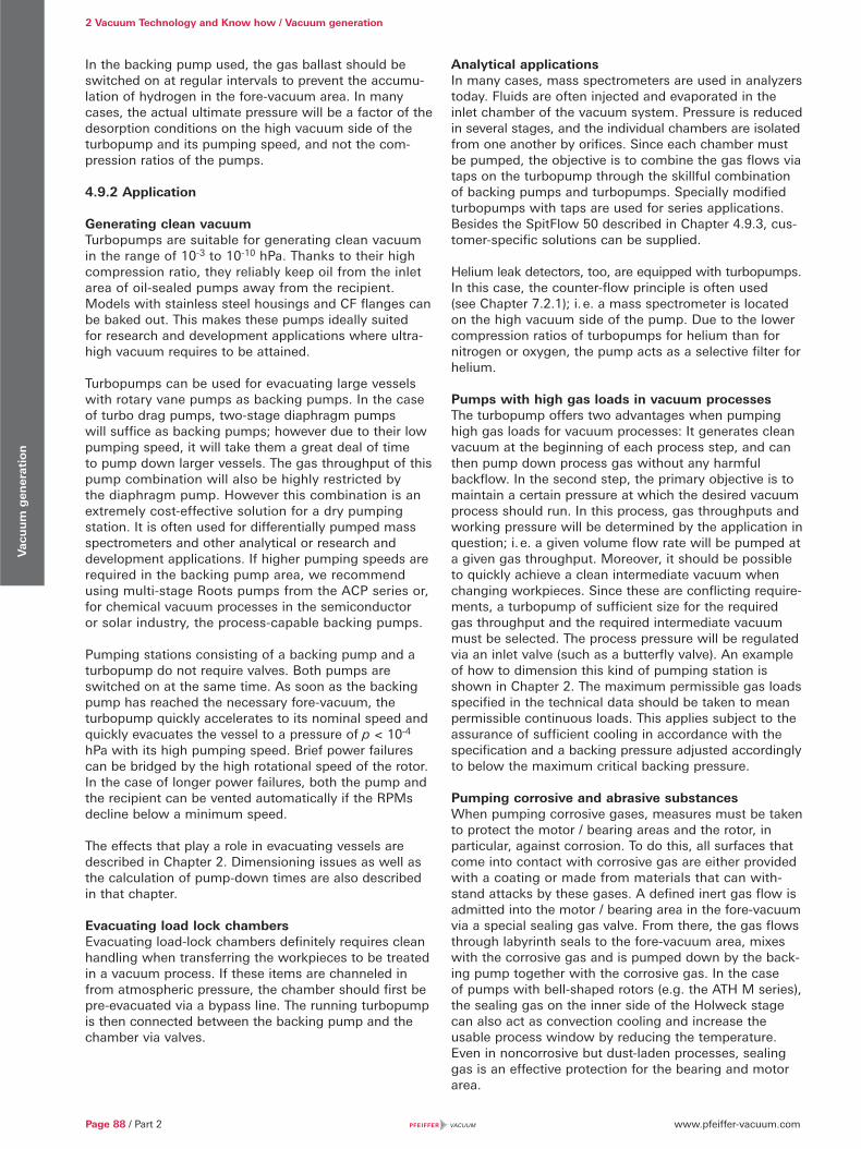
www.pfeiffer-vacuum.comPage 88 / Part 2
2 Vacuum Technology and Know how / Vacuum generationV
acu
um
gen
erat
ion
In the backing pump used, the gas ballast should be switched on at regular intervals to prevent the accumu-lation of hydrogen in the fore-vacuum area. In many cases, the actual ultimate pressure will be a factor of the desorption conditions on the high vacuum side of the turbopump and its pumping speed, and not the com-pression ratios of the pumps.
4.9.2 Application
Generating clean vacuumTurbopumps are suitable for generating clean vacuum in the range of 10-3 to 10-10 hPa. Thanks to their high compression ratio, they reliably keep oil from the inlet area of oil-sealed pumps away from the recipient. Models with stainless steel housings and CF flanges can be baked out. This makes these pumps ideally suited for research and development applications where ultra-high vacuum requires to be attained.
Turbopumps can be used for evacuating large vessels with rotary vane pumps as backing pumps. In the case of turbo drag pumps, two-stage diaphragm pumps will suffice as backing pumps; however due to their low pumping speed, it will take them a great deal of time to pump down larger vessels. The gas throughput of this pump combination will also be highly restricted by the diaphragm pump. However this combination is an extremely cost-effective solution for a dry pumping station. It is often used for differentially pumped mass spectrometers and other analytical or research and development applications. If higher pumping speeds are required in the backing pump area, we recommend using multi-stage Roots pumps from the ACP series or, for chemical vacuum processes in the semiconductor or solar industry, the process-capable backing pumps.
Pumping stations consisting of a backing pump and a turbopump do not require valves. Both pumps are switched on at the same time. As soon as the backing pump has reached the necessary fore-vacuum, the turbopump quickly accelerates to its nominal speed and quickly evacuates the vessel to a pressure of p < 10-4 hPa with its high pumping speed. Brief power failures can be bridged by the high rotational speed of the rotor. In the case of longer power failures, both the pump and the recipient can be vented automatically if the RPMs decline below a minimum speed.
The effects that play a role in evacuating vessels are described in Chapter 2. Dimensioning issues as well as the calculation of pump-down times are also described in that chapter.
Evacuating load lock chambersEvacuating load-lock chambers definitely requires clean handling when transferring the workpieces to be treated in a vacuum process. If these items are channeled in from atmospheric pressure, the chamber should first be pre-evacuated via a bypass line. The running turbopump is then connected between the backing pump and the chamber via valves.
Analytical applicationsIn many cases, mass spectrometers are used in analyzers today. Fluids are often injected and evaporated in the inlet chamber of the vacuum system. Pressure is reduced in several stages, and the individual chambers are isolated from one another by orifices. Since each chamber must be pumped, the objective is to combine the gas flows via taps on the turbopump through the skillful combination of backing pumps and turbopumps. Specially modified turbopumps with taps are used for series applications. Besides the SpitFlow 50 described in Chapter 4.9.3, cus-tomer-specific solutions can be supplied.
Helium leak detectors, too, are equipped with turbopumps. In this case, the counter-flow principle is often used (see Chapter 7.2.1); i. e. a mass spectrometer is located on the high vacuum side of the pump. Due to the lower compression ratios of turbopumps for helium than for nitrogen or oxygen, the pump acts as a selective filter for helium.
Pumps with high gas loads in vacuum processesThe turbopump offers two advantages when pumping high gas loads for vacuum processes: It generates clean vacuum at the beginning of each process step, and can then pump down process gas without any harmful backflow. In the second step, the primary objective is to maintain a certain pressure at which the desired vacuum process should run. In this process, gas throughputs and working pressure will be determined by the application in question; i. e. a given volume flow rate will be pumped at a given gas throughput. Moreover, it should be possible to quickly achieve a clean intermediate vacuum when changing workpieces. Since these are conflicting require-ments, a turbopump of sufficient size for the required gas throughput and the required intermediate vacuum must be selected. The process pressure will be regulated via an inlet valve (such as a butterfly valve). An example of how to dimension this kind of pumping station is shown in Chapter 2. The maximum permissible gas loads specified in the technical data should be taken to mean permissible continuous loads. This applies subject to the assurance of sufficient cooling in accordance with the specification and a backing pressure adjusted accordingly to below the maximum critical backing pressure.
Pumping corrosive and abrasive substances When pumping corrosive gases, measures must be taken to protect the motor / bearing areas and the rotor, in particular, against corrosion. To do this, all surfaces that come into contact with corrosive gas are either provided with a coating or made from materials that can with-stand attacks by these gases. A defined inert gas flow is admitted into the motor / bearing area in the fore-vacuum via a special sealing gas valve. From there, the gas flows through labyrinth seals to the fore-vacuum area, mixes with the corrosive gas and is pumped down by the back-ing pump together with the corrosive gas. In the case of pumps with bell-shaped rotors (e.g. the ATH M series), the sealing gas on the inner side of the Holweck stage can also act as convection cooling and increase the usable process window by reducing the temperature. Even in noncorrosive but dust-laden processes, sealing gas is an effective protection for the bearing and motor area.
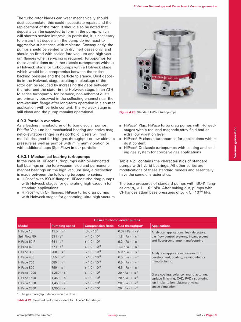
www.pfeiffer-vacuum.com
2 Vacuum Technology and Know how / Vacuum generation
Part 2 / Page 89
Vac
uu
m g
ener
atio
n
The turbo-rotor blades can wear mechanically should dust accumulate; this could necessitate repairs and the replacement of the rotor. It should also be noted that deposits can be expected to form in the pump, which will shorten service intervals. In particular, it is necessary to ensure that deposits in the pump do not react to aggressive substances with moisture. Consequently, the pumps should be vented with dry inert gases only, and should be fitted with sealed fore-vacuum and high vacu-um flanges when servicing is required. Turbopumps for these applications are either classic turbopumps without a Holweck stage, or turbopumps with a Holweck stage which would be a compromise between the critical backing pressure and the particle tolerance. Dust depos-its in the Holweck stage resulting in blockage of the rotor can be reduced by increasing the gaps between the rotor and the stator in the Holweck stage. In an ATH M series turbopump, for instance, non-adherent dusts are primarily observed in the collecting channel near the fore-vacuum flange after long-term operation in a sputter application with particle content. The Holweck stage is still clean and the pump remains operational.
4.9.3 Portfolio overviewAs a leading manufacturer of turbomolecular pumps, Pfeiffer Vacuum has mechanical-bearing and active mag-netic-levitation ranges in its portfolio. Users will find models designed for high gas throughput or low ultimate pressure as well as pumps with minimum vibration or with additional taps (SplitFlow) in our portfolio.
4.9.3.1 Mechanical-bearing turbopumpsIn the case of HiPace® turbopumps with oil-lubricated ball bearings on the fore-vacuum side and permanent-magnet bearings on the high vacuum side, a distinction is made between the following turbopump series:
HiPace® with ISO-K flanges: HiPace turbo drag pumps with Holweck stages for generating high vacuum for standard applications
HiPace® with CF flanges: HiPace turbo drag pumps with Holweck stages for generating ultra-high vacuum
HiPace® Plus: HiPace turbo drag pumps with Holweck stages with a reduced magnetic stray field and an extra low vibration level
HiPace® P: classic turbopumps for applications with a dust content
HiPace® C: classic turbopumps with coating and seal-ing gas system for corrosive gas applications
Table 4.21 contains the characteristics of standard pumps with hybrid bearings. All other series are modifications of these standard models and essentially have the same characteristics.
The base pressures of standard pumps with ISO-K flang-es are: pb < 1 · 10-7 hPa. After baking out, pumps with CF flanges attain base pressures of pb < 5 · 10-10 hPa.
HiPace turbomolecular pumps
Model Pumping speed Compression Ratio Gas throughput* Applications
HiPace 10 11.5 l · s-1 3.0 · 107 0.37 hPa · l · s-1Analytical applications, leak detectors, gas flow control systems, incandescent and fluorescent lamp manufacturing
SplitFlow 50 53 l · s-1 > 1.0 · 108 1.8 hPa · l · s-1
HiPace 60 P 64 l · s-1 > 1.0 · 106 9.2 hPa · l · s-1
HiPace 80 67 l · s-1 > 1.0 · 1011 1.3 hPa · l · s-1
Analytical applications, research & development, coating, semiconductor manufacturing
HiPace 300 260 l · s-1 > 1.0 · 1011 5.0 hPa · l · s-1
HiPace 400 355 l · s-1 > 1.0 · 1011 6.5 hPa · l · s-1
HiPace 700 685 l · s-1 > 1.0 · 1011 6.5 hPa · l · s-1
HiPace 800 790 l · s-1 > 1.0 · 1011 6.5 hPa · l · s-1
HiPace 1200 1,250 l · s-1 > 1.0 · 108 20 hPa · l · s-1Glass coating, solar cell manufacturing, surface finishing, CVD, PVD / sputtering, ion implantation, plasma physics, space simulation
HiPace 1500 1,450 l · s-1 > 1.0 · 108 20 hPa · l · s-1
HiPace 1800 1,450 l · s-1 > 1.0 · 108 20 hPa · l · s-1
HiPace 2300 1,900 l · s-1 > 1.0 · 108 20 hPa · l · s-1
*) The gas throughput depends on the drive.
Table 4.21: Selected performance data for HiPace® for nitrogen
Figure 4.29: Standard HiPace turbopumps

www.pfeiffer-vacuum.comPage 90 / Part 2
2 Vacuum Technology and Know how / Vacuum generationV
acu
um
gen
erat
ion
4.9.3.2 Active magnetic-levitation turbopumpsTable 4.22 contains the characteristics of turbopumps with active 5-axis magnetically levitated bearings. These pumps, too, are available as:
HiPace® M with ISO-K or ISO-F flanges: HiPace turbo drag pumps with Holweck stages for generating high vacuum for standard applications
HiPace® M with CF flanges: HiPace turbo drag pumps with Holweck stages for generating ultra-high vacuum
ATP M: classic turbopumps without Holweck stages with a high compression ratio for light gases and a high particle tolerance
ATH M and MT: Turbo drag pumps with Holweck stages, sealing gas system and heating for corrosive gas applications
4.9.3.3 Drives and accessoriesA variety of controls, displays and drives are available for operating turbopumps in different applications as well as extensive accessories.
The numbering used below is based upon Figure 4.31.
Turbopumps (1a) are generally equipped with an attached drive (1b). The DC power supply comes, for example, from a plug-in power supply module (2a) with a display control unit (2b). Built-in power supply units are also available. A USB converter (5b) can also be used to con-nect a PC (5a) to the RS-485 interface in order to exe-cute programming and switching functions or to transfer status displays. Profibus DP and DeviceNet converters allow the pumps to be linked to system controllers. The major switching functions can also be executed via a remote control plug using external signals. Moreover, some status displays can be taken from relay outputs.
In addition to the operating devices, various accessories are also available for special applications.
Some DCU power supply units enable a vacuum gauge to be connected in order to show the pressure as well as information on the turbopump.
With the aid of the backing pump relay box (6) the DCU power supply (2a) can be converted to a pumping station controller that can switch on both turbopump (1a) and backing pump simultaneously.
Either a fan (4), or water cooling (3) for high gas loads, can be attached to cool the pumps.
An electric vent valve (8) vents the turbopumps if the RPM declines below a given speed. In the event of a brief power failure, the vent valve will remain closed to maintain the vacuum. The pumping station will then re-start immediately when mains voltage is restored. However this necessitates a backing pump with a safety valve that will close automatically in the event of a power failure.
For UHV applications, a heater (9) can be connected to the pump that switches on automatically after a prese-lected rotation speed is attained, and switches off when the rpm decreases.
Figure 4.30: ATH M magnetic-levitation turbopump
Magnetic-levitation turbopump
Model Pumping speed Compression ratio Gas throughput* Applications
HiPace 300 M 255 l · s-1 > 1 · 1011 28 hPa · l · s-1 Analytics, coating, R&D
ATH 500 M / MT 520 l · s-1 > 2 · 107 67 hPa · l · s-1 Semiconductors, coating, R&D
HiPace 700 M 685 l · s-1 > 1 · 1011 13 hPa · l · s-1
Analytics, coating, R&DHiPace 800 M 790 l · s-1 > 1 · 1011 13 hPa · l · s-1
ATH 1603 M 1,370 l · s-1 > 6 · 108 67 hPa · l · s-1
Semiconductors, coating, R&D: Glass coating, solar cell manufacturing, surface finishing, CVD, PVD / sputtering, ion implantation, plasma physics
ATH 1600 MT 1,370 l · s-1 > 5 · 108 67 hPa · l · s-1
ATH 2303 M 1,950 l · s-1 > 1 · 108 67 hPa · l · s-1
ATH 2300 MT 1,950 l · s-1 > 1 · 108 67 hPa · l · s-1
ATP 2300 M 1,850 l · s-1 > 1 · 108 37 hPa · l · s-1
ATH 2800 M 2,150 l · s-1 > 1 · 108 84 hPa · l · s-1
ATH 2800 MT 2,150 l · s-1 > 1 · 108 84 hPa · l · s-1
ATH 3200 M 2,700 l · s-1 > 1 · 108 84 hPa · l · s-1
ATH 3200 MT 2,700 l · s-1 > 1 · 108 84 hPa · l · s-1
*) The gas throughput depends on the drive.
Table 4.22: Performance data for magnetic-bearing turbopumps for nitrogen

www.pfeiffer-vacuum.com
2 Vacuum Technology and Know how / Vacuum generation
Part 2 / Page 91
Vac
uu
m g
ener
atio
n
2a
1a
4
9
5a
8
7a 7b3
6
5b
2b 1b
1a) Turbopump
1b) TC 400 drive
2a) DCU power supply
2b) DCU 002
3) Water cooling
4) Air cooling
5a) PC
5b) USB converter
6) Backing pump relay box
7a) Sealing gas throttles
7b) Sealing gas valve
8) Venting valve
9) Heater
Electromagnetic sealing gas valves (7b) with matching throughputs, as well as sealing gas throttles (7a) for pumps of various sizes, are available for corrosive gas pumps.
Please refer to Chapter 3.1 Turbopumps in our product catalog for further details.
Figure 4.31: Example of turbopump accessories (for HiPace 300)

www.pfeiffer-vacuum.comPage 92 / Part 2
Vac
uu
m m
easu
rin
g
equ
ipm
ent
5 Vacuum measuring equipment
5.1 Fundamentals of total pressure measurement
Pressure is defined as force per unit of area: p = F/A (Formula 1-3) where F is the force and A the area to which the force is applied. The SI unit of pressure is 1 N / m² = 1 Pa. Other frequently-used units of pressure are: 1 mbar = 1 hPa = 100 Pa and 1 Torr = 133,322 Pa. If pressure is measured via the force that is exerted on an area, the pressure measurement is independent of the type of gas. A tool for converting all units of pressure commonly used in vacuum technology can be found in the Pfeiffer Vacuum app for smartphones (visit www.pfeiffer-vacuum.com).
Pressure measurement on the basis of force reaches its limits at pressures of less than 1 hPa, because the exerted forces become too small. Consequently other processes must be used. The thermal conductivity of the enclosed gas can be used, for example, or the gas molecules can be ionized and the ion current flowing between electrodes measured. These indirect measurements which determine the pressure from a gas property consequently deliver a measurement result that is dependent on the type of gas.
In vacuum technology, no single measurement method covers the entire pressure range. It is therefore necessary to use different sensors. The criteria for selecting a pressure sensor are based upon various conditions:
The pressure range to be detected Gas composition: Inert or corrosive Required accuracy and repeatability Environmental conditions, such as radioactivity
5.1.1 Direct, gas-independent pressure measurementIn the case of a diaphragm vacuum gauge, pressure is measured in accordance with the definition. A pressure p is exerted on a diaphragm having a defined area A and deflects the diaphragm proportionally to the pressure. A sensor measures the deflection; in the most straight-forward case, the deflection is transmitted mechanically to the needle moving over a pressure dial. Piezo-resistive or capacitive sensors receive the pressure signal and convert it into an electrical signal.
Piezo-diaphragm vacuum gaugesA simple and extremely robust method involves the use of a piezo-resistive pick-up. The design is shown in Figure 5.1. A diaphragm into which strain resistances have been diffused is arranged over an evacu ated volume having a reference pressure p0. The measured change in resistance as a result of diaphragm deflection serves as a parameter for the pressure. This sensor is characterized by its insensitivity to gas inrush and its high accuracy.
Figure 5.1: Design of a diaphragm vacuum gauge
Capacitive diaphragm vacuum gaugesIn a capacitive vacuum gauge (Figure 3.2), deflection of the diaphragm is measured as the change in capacity of a plate capacitor that is formed by the diaphragm and a fixed counter-electrode in a well-evacuated space having a pressure p0. The diaphragm is comprised either of ceramics with a vacuum-metalized coating or of stainless steel. This method and diaphragms of varying sensitivity can be used to perform measurements of four decades each. The lower measurement limit is 10-5 hPa.
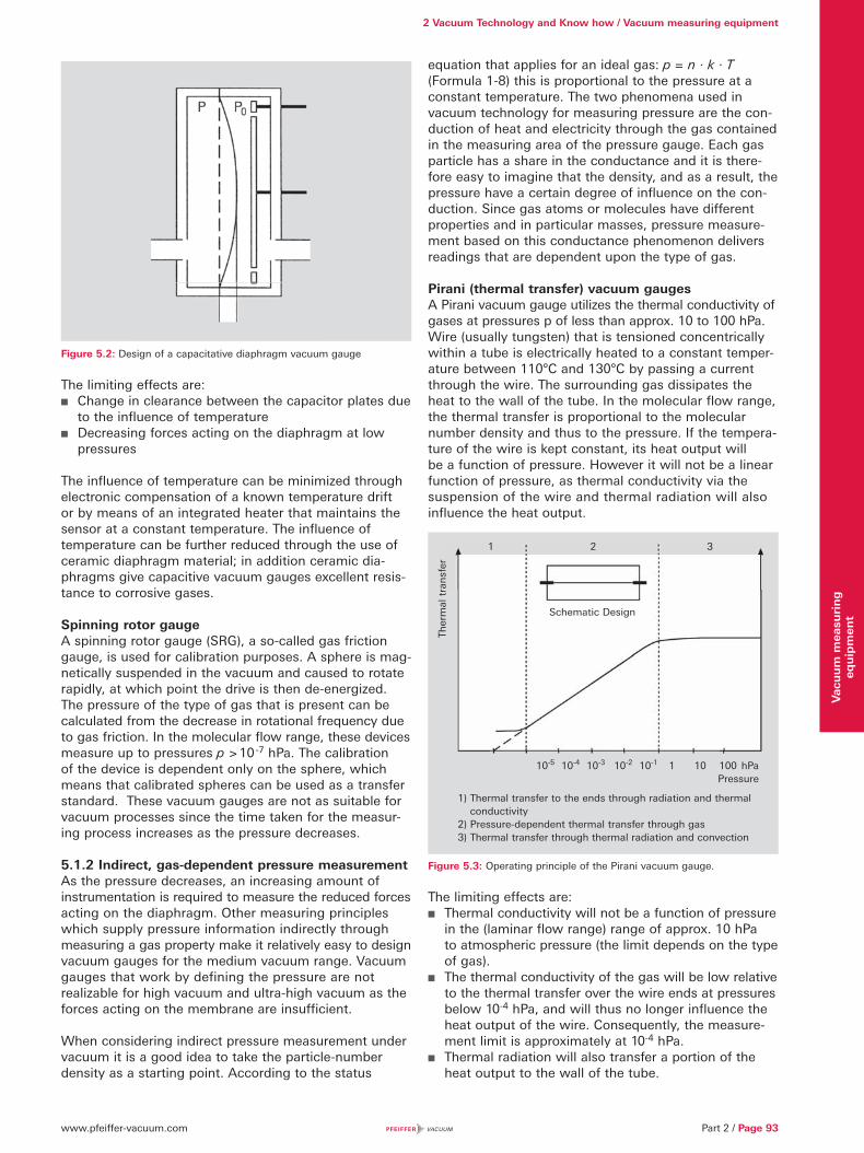
www.pfeiffer-vacuum.com Part 2 / Page 93
2 Vacuum Technology and Know how / Vacuum measuring equipment
Vac
uu
m m
easu
rin
g
equ
ipm
ent
equation that applies for an ideal gas: p = n · k · T (Formula 1-8) this is proportional to the pressure at a constant temperature. The two phenomena used in vacuum technology for measuring pressure are the con-duction of heat and electricity through the gas contained in the measuring area of the pressure gauge. Each gas particle has a share in the conductance and it is there-fore easy to imagine that the density, and as a result, the pressure have a certain degree of influence on the con-duction. Since gas atoms or molecules have different properties and in particular masses, pressure measure-ment based on this conductance phenomenon delivers readings that are dependent upon the type of gas.
Pirani (thermal transfer) vacuum gaugesA Pirani vacuum gauge utilizes the thermal conductivity of gases at pressures p of less than approx. 10 to 100 hPa. Wire (usually tungsten) that is tensioned concentrically within a tube is electrically heated to a constant temper-ature between 110°C and 130°C by passing a current through the wire. The surrounding gas dissipates the heat to the wall of the tube. In the molecular flow range, the thermal transfer is proportional to the molecular number density and thus to the pressure. If the tempera-ture of the wire is kept constant, its heat output will be a function of pressure. However it will not be a linear function of pressure, as thermal conductivity via the suspension of the wire and thermal radiation will also influence the heat output.
Figure 5.3: Operating principle of the Pirani vacuum gauge.
The limiting effects are: Thermal conductivity will not be a function of pressure
in the (laminar flow range) range of approx. 10 hPa to atmospheric pressure (the limit depends on the type of gas).
The thermal conductivity of the gas will be low relative to the thermal transfer over the wire ends at pressures below 10-4 hPa, and will thus no longer influence the heat output of the wire. Consequently, the measure-ment limit is approximately at 10-4 hPa.
Thermal radiation will also transfer a portion of the heat output to the wall of the tube.
Figure 5.2: Design of a capacitative diaphragm vacuum gauge
The limiting effects are: Change in clearance between the capacitor plates due
to the influence of temperature Decreasing forces acting on the diaphragm at low
pressures
The influence of temperature can be minimized through electronic compensation of a known temperature drift or by means of an integrated heater that maintains the sensor at a constant temperature. The influence of temperature can be further reduced through the use of ceramic diaphragm material; in addition ceramic dia-phragms give capacitive vacuum gauges excellent resis-tance to corrosive gases.
Spinning rotor gaugeA spinning rotor gauge (SRG), a so-called gas friction gauge, is used for calibration purposes. A sphere is mag-netically suspended in the vacuum and caused to rotate rapidly, at which point the drive is then de-energized. The pressure of the type of gas that is present can be calculated from the decrease in rotational frequency due to gas friction. In the molecular flow range, these devices measure up to pressures p > 10 -7 hPa. The calibration of the device is dependent only on the sphere, which means that calibrated spheres can be used as a transfer standard. These vacuum gauges are not as suitable for vacuum processes since the time taken for the measur-ing process increases as the pressure decreases.
5.1.2 Indirect, gas-dependent pressure measurementAs the pressure decreases, an increasing amount of instrumentation is required to measure the reduced forces acting on the diaphragm. Other measuring principles which supply pressure information indirectly through measuring a gas property make it relatively easy to design vacuum gauges for the medium vacuum range. Vacuum gauges that work by defining the pressure are not realizable for high vacuum and ultra-high vacuum as the forces acting on the membrane are insufficient.
When considering indirect pressure measurement under vacuum it is a good idea to take the particle-number density as a starting point. According to the status
1) Thermal transfer to the ends through radiation and thermal conductivity
2) Pressure-dependent thermal transfer through gas 3) Thermal transfer through thermal radiation and convection
Ther
mal
tra
nsf
er
1 2 3
Schematic Design
10-5 10-4 10-3 10-2 10-1 1 10 100 hPaPressure
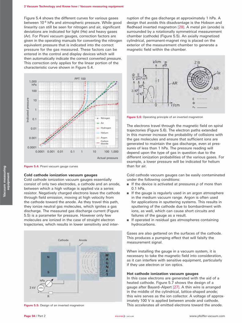
www.pfeiffer-vacuum.comPage 94 / Part 2
2 Vacuum Technology and Know how / Vacuum measuring equipmentV
acu
um
mea
suri
ng
eq
uip
men
t
Figure 5.4 shows the different curves for various gases between 10-4 hPa and atmospheric pressure. While good linearity can still be seen for nitrogen and air, significant deviations are indicated for light (He) and heavy gases (Ar). For Pirani vacuum gauges, correction factors are given in the operating manuals for converting the nitrogen equivalent pressure that is indicated into the correct pressure for the gas measured. These factors can be entered in the control and display devices which will then automatically indicate the correct converted pressure. This correction only applies for the linear portion of the characteristic curve shown in Figure 5.4.
Figure 5.4: Pirani vacuum gauge curves
Cold cathode ionization vacuum gaugesCold cathode ionization vacuum gau ges essentially consist of only two electrodes, a cathode and an anode, between which a high voltage is applied via a series resistor. Negatively charged electrons leave the cathode through field emission, moving at high velocity from the cathode toward the anode. As they travel this path, they ionize neutral gas molecules, which ignites a gas discharge. The measured gas discharge current (Figure 5.5) is a parameter for pressure. However only few molecules are ionized in the case of straight electron trajectories, which results in lower sensitivity and inter-
ruption of the gas discharge at approximately 1 hPa. A design that avoids this disadvantage is the Hobson and Redhead inverted magnetron [28]. A metal pin (anode) is surrounded by a rotationally symmetrical measurement chamber (cathode) (Figure 5.5). An axially magnetized cylindrical, permanent-magnet ring is placed on the exterior of the measurement chamber to generate a magnetic field within the chamber.
Figure 5.6: Operating principle of an inverted magnetron
The electrons travel through the mag netic field on spiral trajectories (Figure 5.6). The electron paths extended in this manner increase the probability of collisions with the gas molecules and ensure that sufficient ions are generated to maintain the gas discharge, even at pres-sures of less than 1 hPa. The pressure reading will depend upon the type of gas in question due to the different ionization probabilities of the various gases. For example, a lower pressure will be indicated for helium than for air.
Cold cathode vacuum gauges can be easily contaminated under the following conditions:
If the device is activated at pressures p of more than 0.1 hPa.
If the gauge is regularly used in an argon atmosphere in the medium vacuum range. Argon is often used for applications in sputtering systems. This results in sputtering of the cathode due to bombardment with ions, as well, which can cause short circuits and failures of the gauge as a result.
If operated in residual gas atmospheres containing hydrocarbons.
Gases are also gettered on the surfaces of the cathode. This produces a pumping effect that will falsify the measurement signal.
When installing the gauge in a vacuum system, it is necessary to take the magnetic field into consideration, as it can interfere with sensitive equipment, particularly if they use electron or ion optics.
Hot cathode ionization vacuum gaugesIn this case electrons are generated with the aid of a heated cathode. Figure 5.7 shows the design of a gauge after Bayard–Alpert [27]. A thin wire is arranged in the middle of the cylindrical, lattice-shaped anode; this wire serves as the ion collector. A voltage of approx-imately 100 V is applied between anode and cathode. This accelerates all emitted electrons toward the anode. Figure 5.5: Design of an inverted magnetron
Actual pressure
PPT 1001,000
hPa
100
10
1
0.1
0.01
0.001
0.0001
Ind
icat
ed p
ress
ure
Nitrogen
Air
Hydrogen
Helium
Argon
Carbon dioxide
0.0001 0.001 0.01 0.1 1 10 100 1,000
AnodeCathode
N
S
3 kV
R
hPa
+
E
ne
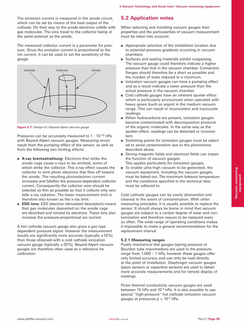
www.pfeiffer-vacuum.com Part 2 / Page 95
2 Vacuum Technology and Know how / Vacuum measuring equipment
Vac
uu
m m
easu
rin
g
equ
ipm
ent
The emission current is measured in the anode circuit, which can be set by means of the heat output of the cathode. On their way to the anode electrons collide with gas molecules. The ions travel to the collector being at the same potenial as the anode.
The measured collector current is a parameter for pres-sure. Since the emission current is proportional to the ion current, it can be used to set the sensitivity of the gauge.
Figure 5.7: Design of a Bayard-Alpert vacuum gauge
Pressures can be accurately measured to 1 · 10-10 hPa with Bayard-Alpert vacuum gauges. Measuring errors resul t from the pumping effect of the sensor, as well as from the following two limiting effects:
X-ray bremsstrahlung: Electrons that strike the anode cage cause x-rays to be emitted, some of which strike the collector. This x-ray effect causes the collector to emit photo electrons that flow off toward the anode. The resulting photoelectron current increases and falsifies the pressure-dependent collector current. Consequently the collector wire should be selected as thin as possible so that it collects only very little x-ray radiation. The lower measurement limit is therefore also known as the x-ray limit.
ESD ions: ESD (electron stimulated desorption) means that gas molecules deposited on the anode cage are desorbed and ionized by electrons. These ions also increase the pressure-proportional ion current.
A hot cathode vacuum gauge also gives a gas type dependent pressure signal. However the measurement results are significantly more accurate (typically ±10 %) than those obtained with a cold cathode ionization vacuum gauge (typically ± 25 %). Bayard-Alpert vacuum gauges are therefore often used as a reference for calibration.
5.2 Application notes
When selecting and installing vacuum gauges their properties and the particularities of vacuum measurement must be taken into account:
Appropriate selection of the installation location due to potential pressure gradients occurring in vacuum chambers.
Surfaces and sealing materials exhibit outgassing. The vacuum gauge could therefore indicate a higher pressure than that in the vacuum chamber. Connection flanges should therefore be a short as possible and the number of seals reduced to a minimum.
Ionization vacuum gauges can have a pumping effect and as a result indicate a lower pressure than the actual pressure in the vacuum chamber.
Cold cathode gauges have an inherent sputter effect which is particularly pronounced when operated with heavy gases (such as argon) in the medium vacuum range. This can result in inconsistent and inaccurate readings.
When hydrocarbons are present, ionization gauges become contaminated with decomposition products of the organic molecules. In the same way as the sputter effect, readings can be distorted or inconsis-tent.
Switching points for ionization gauges must be select-ed to avoid contamination due to the phenomena described above.
Strong magnetic fields and electrical fields can impair the function of vacuum gauges. This applies particularly for ionization gauges.
To enable ultra-high vacuum to be generated, the vacuum equipment, including the vacuum gauges, must be baked out. The maximum bakeout temperature and the conditions specified in the technical data must be adhered to.
Cold cathode gauges can be easily dismantled and cleaned in the event of contamination. With other measuring principles, it is usually possible to replace the sensor. It should always be borne in mind that vacuum gauges are subject to a certain degree of wear and con-tamination and therefore require to be replaced every so often. The wide range of operating conditions makes it impossible to make a general recommendation for the replacement interval.
5.2.1 Measuring rangesPurely mechanical dial gauges (spring pressure or Bourdon tube manometers) are used in the pressure range from 1,000 – 1 hPa; however these gauges offer only limited accuracy and can only be read directly at the point of installation. Diaphragm vacuum gauges (piezo sensors or capacitive sensors) are used to obtain more accurate measurements and for remote display of readings.
Pirani thermal conductivity vacuum gauges are used between 10 hPa and 10-4 hPa. It is also possible to use special “high-pressure” hot cathode ionization vacuum gauges at pressures p < 10-2 hPa.
Cathode Collector Anode
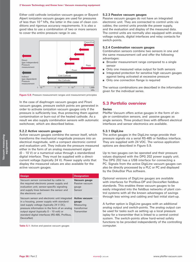
www.pfeiffer-vacuum.comPage 96 / Part 2
2 Vacuum Technology and Know how / Vacuum measuring equipmentV
acu
um
mea
suri
ng
eq
uip
men
t
Either cold cathode ionization vacuum gauges or Bayard-Alpert ionization vacuum gauges are used for pressures of less than 10-3 hPa, the latter in the case of clean con-ditions and rigorous accuracy requirements. It is also a good idea to use a combination of two or more sensors to cover the entire pressure range in use.
Figure 5.8: Pressure measurement ranges and measurement principles
In the case of diaphragm vacuum gauges and Pirani vacuum gauges, pressure switch points are generated in order to activate ionization vacuum gauges only if the pressure is sufficiently low, thus protecting them against contamination or burn-out of the heated cathode. As a result we also supply combination sensors with automatic switchover, which are described below.
5.2.2 Active vacuum gaugesActive vacuum gauges combine the sensor itself, which transforms the mechanical magnitude pressure into an electrical magnitude, with a compact electronic control and evaluation unit. They indicate the pressure measured either in the form of an analog measurement signal (0 – 10 V) or a numerical value through a standardized digital interface. They must be supplied with a direct- current voltage (typically 24 V). Power supply units that display the measured values are also available for the active vacuum gauges.
Design Designation
Vacuum sensor connected by cable to the required electronic power supply and evaluation unit; sensor-specific signaling and supply lines between the sensor and the electronic unit
Vacuum gaugePassive vacuum gaugeSensor
Vacuum sensor and electronic unit integrated in a housing, power supply with standard-ized supply voltage (typically 24 V DC); pressure information in the form of an analog output signal (typically 0 – 10 volt) or standard digital interfaces (RS-485, Profibus, DeviceNet)
Active vacuum gaugeMeasuring transformerTransmitter
Table 5.1: Active and passive vacuum gauges
5.2.3 Passive vacuum gaugesPassive vacuum gauges do not have an integrated electronic unit. They are connected to control units via cables; the control units provide the power supply, and the evaluation and display of the measured data. The control units are normally also equipped with analog voltage outputs, digital interfaces and relay contacts for switch-points.
5.2.4 Combination vacuum gaugesCombination sensors combine two sensors in one and the same measurement cell and offer the following advantages:
Broader measurement range compared to a single sensor
Only one measured value output for both sensors Integrated protection for sensitive high vacuum gauges
against being activated at excessive pressure Only one connection flange is required
The various combinations are described in the information given for the individual series.
5.3 Portfolio overviewSeriesPfeiffer Vacuum offers active gauges in the form of sin-gle or combination sensors, and passive gauges as single sensors. Three product lines with different electrical interfaces and sensor electronics are available.
5.3.1 DigiLineThe active gauges in the DigiLine range provide their pressure signals via a serial RS-485 or fieldbus interface. They are supplied with 24 VDC. The various application options are described in Figure 5.9.
Up to two gauges can be operated and their pressure values displayed with the DPG 202 power supply unit. The DPG 202 has a USB interface for connecting a PC. Signals from the active DigiLine vacuum gauges can also be directly processed by a PLC or PC and displayed by the DokuStar Plus software.
Optional versions of DigiLine gauges are available with interfaces for Profibus-DP and DeviceNet fieldbus standards. This enables these vacuum gauges to be easily integrated into the fieldbus networks of plant con-trol systems with all the known advantages of savings through less wiring and cabling and fast initial start-up.
A further option is DigiLine gauges with an additional analog output and switch-points. The analog output can be used for tasks such as setting up a local pressure isplay for a transmitter that is linked to a central control system. The switch-points allow hard-wired safety functions to be provided independently of the controlling computer.
Capacitive
Piezo
Pirani
Cold Cathode
Hot Cathode
Direct(gas independent)Pressure measurement
Indirect(gas dependent)Pressure measurement
1 · 10 -13 1 · 10 -7 1 · 10 -3 1 1,000hPa
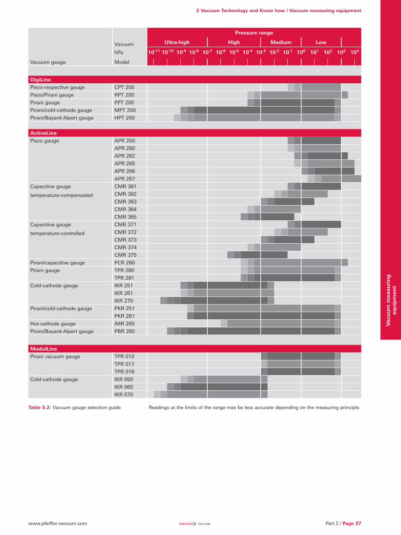
www.pfeiffer-vacuum.com Part 2 / Page 97
2 Vacuum Technology and Know how / Vacuum measuring equipment
Vac
uu
m m
easu
rin
g
equ
ipm
ent
Pressure range
Vacuum Ultra-high High Medium Low
hPa 10-11 10-10 10-9 10-8 10-7 10-6 10-5 10-4 10-3 10-2 10-1 100 101 102 103 104
Vacuum gauge Model
DigiLine
Piezo-respective gauge CPT 200
Piezo/Pirani gauge RPT 200
Pirani gauge PPT 200
Pirani/cold-cathode gauge MPT 200
Pirani/Bayard-Alpert gauge HPT 200
ActiveLine
Piezo gauge APR 250
APR 260
APR 262
APR 265
APR 266
APR 267
Capacitive gauge
temperature-compensated
CMR 361
CMR 362
CMR 363
CMR 364
CMR 365
Capacitive gauge
temperature-controlled
CMR 371
CMR 372
CMR 373
CMR 374
CMR 375
Pirani/capacitive gauge PCR 280
Pirani gauge TPR 280
TPR 281
Cold-cathode gauge IKR 251
IKR 261
IKR 270
Pirani/cold-cathode gauge PKR 251
PKR 261
Hot-cathode gauge IMR 265
Pirani/Bayard-Alpert gauge PBR 260
ModulLine
Pirani vacuum gauge TPR 010
TPR 017
TPR 018
Cold-cathode gauge IKR 050
IKR 060
IKR 070
Table 5.2: Vacuum gauge selection guide Readings at the limits of the range may be less accurate depending on the measuring principle.
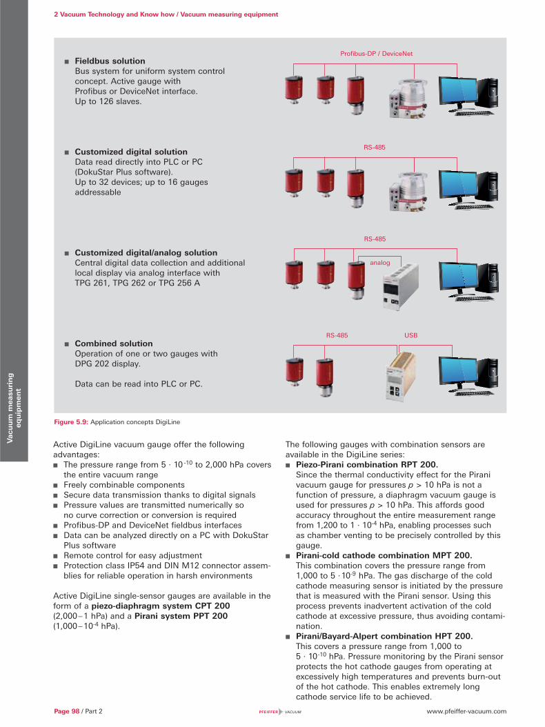
www.pfeiffer-vacuum.comPage 98 / Part 2
2 Vacuum Technology and Know how / Vacuum measuring equipmentV
acu
um
mea
suri
ng
eq
uip
men
t
Active DigiLine vacuum gauge offer the following advantages:
The pressure range from 5 · 10 -10 to 2,000 hPa covers the entire vacuum range
Freely combinable components Secure data transmission thanks to digital signals Pressure values are transmitted numerically so
no curve correction or conversion is required Profibus-DP and DeviceNet fieldbus interfaces Data can be analyzed directly on a PC with DokuStar
Plus software Remote control for easy adjustment Protection class IP54 and DIN M12 connector assem-
blies for reliable operation in harsh environments
Active DigiLine single-sensor gauges are available in the form of a piezo-diaphragm system CPT 200 (2,000 – 1 hPa) and a Pirani system PPT 200 (1,000 – 10-4 hPa).
The following gauges with combination sensors are available in the DigiLine series:
Piezo-Pirani combination RPT 200. Since the thermal conductivity effect for the Pirani vacuum gauge for pressures p > 10 hPa is not a function of pressure, a diaphragm vacuum gauge is used for pressures p > 10 hPa. This affords good accuracy throughout the entire measurement range from 1,200 to 1 · 10-4 hPa, enabling processes such as chamber venting to be precisely controlled by this gauge.
Pirani-cold cathode combination MPT 200. This combination covers the pressure range from 1,000 to 5 · 10-9 hPa. The gas discharge of the cold cathode measuring sensor is initiated by the pressure that is measured with the Pirani sensor. Using this process prevents inadvertent activation of the cold cathode at excessive pressure, thus avoiding contami-nation.
Pirani/Bayard-Alpert combination HPT 200. This covers a pressure range from 1,000 to 5 · 10-10 hPa. Pressure monitoring by the Pirani sensor protects the hot cathode gauges from operating at excessively high temperatures and prevents burn-out of the hot cathode. This enables extremely long cathode service life to be achieved.
Figure 5.9: Application concepts DigiLine
Fieldbus solution Bus system for uniform system control concept. Active gauge with Profibus or DeviceNet interface. Up to 126 slaves.
Customized digital solution Data read directly into PLC or PC (DokuStar Plus software). Up to 32 devices; up to 16 gauges addressable
Customized digital/analog solution Central digital data collection and additional local display via analog interface with TPG 261, TPG 262 or TPG 256 A
Combined solution Operation of one or two gauges with DPG 202 display. Data can be read into PLC or PC.
Profibus-DP / DeviceNet
RS-485
RS-485 USB
RS-485
analog
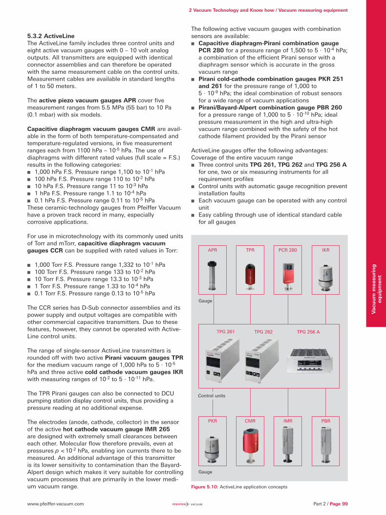
www.pfeiffer-vacuum.com Part 2 / Page 99
2 Vacuum Technology and Know how / Vacuum measuring equipment
Vac
uu
m m
easu
rin
g
equ
ipm
ent
The following active vacuum gauges with combination sensors are available:
Capacitive diaphragm-Pirani combination gauge PCR 280 for a pressure range of 1,500 to 5 · 10-4 hPa; a combination of the efficient Pirani sensor with a diaphragm sensor which is accurate in the gross vacuum range
Pirani cold-cathode combination gauges PKR 251 and 261 for the pressure range of 1,000 to 5 · 10-9 hPa; the ideal combination of robust sensors for a wide range of vacuum applications
Pirani/Bayard-Alpert combination gauge PBR 260 for a pressure range of 1,000 to 5 · 10-10 hPa; ideal pressure measurement in the high and ultra-high vacuum range combined with the safety of the hot cathode filament provided by the Pirani sensor
ActiveLine gauges offer the following advantages:Coverage of the entire vacuum range
Three control units TPG 261, TPG 262 and TPG 256 A for one, two or six measuring instruments for all requirement profiles
Control units with automatic gauge recognition prevent installation faults
Each vacuum gauge can be operated with any control unit
Easy cabling through use of identical standard cable for all gauges
5.3.2 ActiveLineThe ActiveLine family includes three control units and eight active vacuum gauges with 0 – 10 volt analog outputs. All transmitters are equipped with identical connector assemblies and can therefore be operated with the same measurement cable on the control units. Measurement cables are available in standard lengths of 1 to 50 meters.
The active piezo vacuum gauges APR cover five measurement ranges from 5.5 MPa (55 bar) to 10 Pa (0.1 mbar) with six models.
Capacitive diaphragm vacuum gauges CMR are avail-able in the form of both temperature-compensated and temperature-regulated versions, in five measurement ranges each from 1100 hPa – 10-5 hPa. The use of diaphragms with different rated values (full scale = F.S.) results in the following categories:
1,000 hPa F.S. Pressure range 1,100 to 10-1 hPa 100 hPa F.S. Pressure range 110 to 10-2 hPa 10 hPa F.S. Pressure range 11 to 10-3 hPa 1 hPa F.S. Pressure range 1.1 to 10-4 hPa 0.1 hPa F.S. Pressure range 0.11 to 10-5 hPa
These ceramic-technology gauges from Pfeiffer Vacuum have a proven track record in many, especially corrosive applications.
For use in microtechnology with its commonly used units of Torr and mTorr, capacitive diaphragm vacuum gauges CCR can be supplied with rated values in Torr:
1,000 Torr F.S. Pressure range 1,332 to 10-1 hPa 100 Torr F.S. Pressure range 133 to 10-2 hPa 10 Torr F.S. Pressure range 13.3 to 10-3 hPa 1 Torr F.S. Pressure range 1.33 to 10-4 hPa 0.1 Torr F.S. Pressure range 0.13 to 10-5 hPa
The CCR series has D-Sub connector assemblies and its power supply and output voltages are compatible with other commercial capacitive transmitters. Due to these features, however, they cannot be operated with Active-Line control units.
The range of single-sensor ActiveLine transmitters is rounded off with two active Pirani vacuum gauges TPR for the medium vacuum range of 1,000 hPa to 5 · 10-5 hPa and three active cold cathode vacuum gauges IKR with measuring ranges of 10-2 to 5 · 10-11 hPa.
The TPR Pirani gauges can also be connected to DCU pumping station display control units, thus providing a pressure reading at no additional expense.
The electrodes (anode, cathode, collector) in the sensor of the active hot cathode vacuum gauge IMR 265 are designed with extremely small clearances between each other. Molecular flow therefore prevails, even at pressures p < 10-2 hPa, enabling ion currents there to be measured. An additional advantage of this transmitter is its lower sensitivity to contamination than the Bayard-Alpert design which makes it very suitable for controlling vacuum processes that are primarily in the lower medi-um vacuum range. Figure 5.10: ActiveLine application concepts
APR TPR PCR 280 IKR
PKR CMR IMR PBR
Gauge
Gauge
Control units
TPG 262TPG 261 TPG 256 A
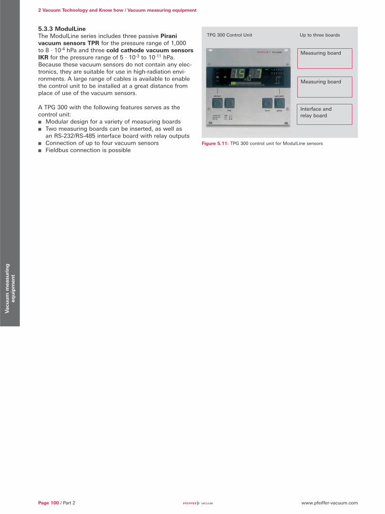
www.pfeiffer-vacuum.comPage 100 / Part 2
2 Vacuum Technology and Know how / Vacuum measuring equipmentV
acu
um
mea
suri
ng
eq
uip
men
t
5.3.3 ModulLineThe ModulLine series includes three passive Pirani vacuum sensors TPR for the pressure range of 1,000 to 8 · 10-4 hPa and three cold cathode vacuum sensors IKR for the pressure range of 5 · 10-3 to 10-11 hPa. Because these vacuum sensors do not contain any elec-tronics, they are suitable for use in high-radiation envi-ronments. A large range of cables is available to enable the control unit to be installed at a great distance from place of use of the vacuum sensors.
A TPG 300 with the following features serves as the control unit:
Modular design for a variety of measuring boards Two measuring boards can be inserted, as well as
an RS-232/RS-485 interface board with relay outputs Connection of up to four vacuum sensors Fieldbus connection is possible
Measuring board
Measuring board
TPG 300 Control Unit Up to three boards
Interface and relay board
Figure 5.11: TPG 300 control unit for ModulLine sensors

www.pfeiffer-vacuum.comPart 2 / Page 101
2 Vacuum Technology and Know how / Vacuum measuring equipment
Vac
uu
m m
easu
rin
g
equ
ipm
ent

www.pfeiffer-vacuum.comPage 102 / Part 2
Mas
s sp
ectr
omet
ers
and
resi
dual
gas
ana
lysi
s
6 Mass spectrometers and residual gas analysis
6.1 Introduction, operating principle
Mass spectrometry is one of the most popular analysis methods. A mass spectrometer analyzes the composition of chemical substances by means of partial pressure measurement under vacuum.
Figure 6.1: Total and partial pressure measurement
Analyses are typically performed in the field of research & development and in the production of products that are used in daily life:
Research & Development Catalysis research Drug development Development of new materials
Monitoring production processes in metallurgy in chemical synthesis in semiconductor production in surface technology
Trace and environmental analysis Aerosol and pollutant monitoring Doping tests Forensic analysis Isotope analysis to identify the origin
Analysis of products in the chemical industry high purity gas production pharmaceuticals the automotive (supply) industry (leak detection) Quality assurance of food products
Mass spectrometers are used to analyze gases. Solid or liquid substances can also be analyzed if they are vaporized in an upstream inlet system. The gas is diluted by pumping it down to a low pressure (molecular flow range) in a vacuum chamber and ionizing it through electron bombardment. The ions thus generated are separated in a mass filter according to their charge-to-mass ratio.
Figure 6.2: Components of a mass spectrometer
Figure 6.2 shows the typical components of a mass spectrometer system.
The substances to be analyzed are admitted to a vacuum chamber through the inlet system via a capillary or metering valve, for example, and then are
pumped down with the vacuum system to the system’s working pressure.
The actual analyzer is located in the vacuum and consists of the following components:
The ion source ionizes neutral gas particles, which are then
separated in the mass filter on the basis of their mass-to-charge ratio m/e.
The ion current is measured using a Faraday detector or a secondary electron multiplier (SEM) after the ions have left the separating system. The current is a measure of the partial pressure of the respective gas molecules or a measure of fragments that may have been generated in the ion source.
Mass and charge Total pressure is the sum of all partial pressures
in a given gas mixture In order to determine the partial pressure of a
certain component of a gas, it must be measured in isolation from the mixture
This necessitates prior separation of the mixture This is accomplished on the basis of the
mass-to-charge ratio m / e
No separation:Total pressure
Separation as a function of time or space: Individual partial pressures
Inlet system Ion source Mass filter Detector
Data analysis system
Vacuum system
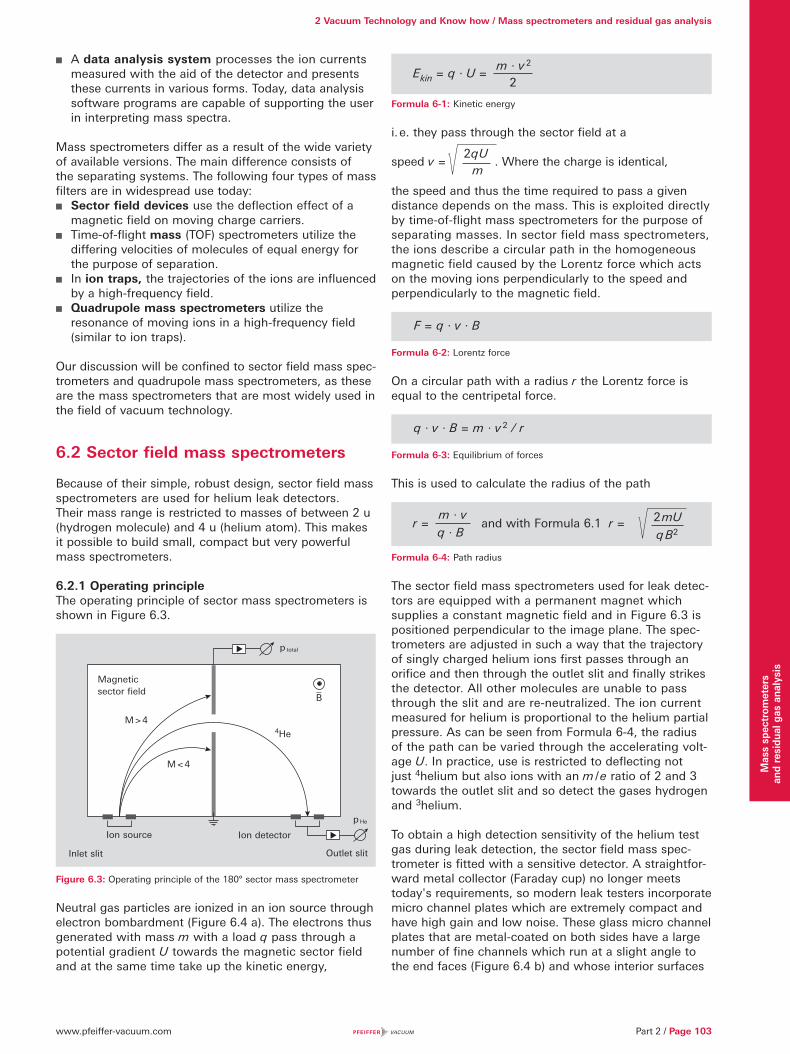
www.pfeiffer-vacuum.com Part 2 / Page 103
2 Vacuum Technology and Know how / Mass spectrometers and residual gas analysis
Mas
s sp
ectr
omet
ers
an
d re
sidu
al g
as a
naly
sis
Formula 6-1: Kinetic energy
i. e. they pass through the sector field at a
speed v = . Where the charge is identical,
the speed and thus the time required to pass a given distance depends on the mass. This is exploited directly by time-of-flight mass spectrometers for the purpose of separating masses. In sector field mass spectrometers, the ions describe a circular path in the homogeneous magnetic field caused by the Lorentz force which acts on the moving ions perpendicularly to the speed and perpendicularly to the magnetic field.
Formula 6-2: Lorentz force
On a circular path with a radius r the Lorentz force is equal to the centripetal force.
Formula 6-3: Equilibrium of forces
This is used to calculate the radius of the path
Formula 6-4: Path radius
The sector field mass spectrometers used for leak detec-tors are equipped with a permanent magnet which supplies a constant magnetic field and in Figure 6.3 is positioned perpendicular to the image plane. The spec-trometers are adjusted in such a way that the trajectory of singly charged helium ions first passes through an orifice and then through the outlet slit and finally strikes the detector. All other molecules are unable to pass through the slit and are re-neutralized. The ion current measured for helium is proportional to the helium partial pressure. As can be seen from Formula 6-4, the radius of the path can be varied through the accelerating volt-age U. In practice, use is restricted to deflecting not just 4helium but also ions with an m / e ratio of 2 and 3 towards the outlet slit and so detect the gases hydrogen and 3helium.
To obtain a high detection sensitivity of the helium test gas during leak detection, the sector field mass spec-trometer is fitted with a sensitive detector. A straightfor-ward metal collector (Faraday cup) no longer meets today's requirements, so modern leak testers incorporate micro channel plates which are extremely compact and have high gain and low noise. These glass micro channel plates that are metal-coated on both sides have a large number of fine channels which run at a slight angle to the end faces (Figure 6.4 b) and whose interior surfaces
A data analysis system processes the ion currents measured with the aid of the detector and presents these currents in various forms. Today, data analysis software programs are capable of supporting the user in interpreting mass spectra.
Mass spectrometers differ as a result of the wide variety of available versions. The main difference consists of the separating systems. The following four types of mass filters are in widespread use today:
Sector field devices use the deflection effect of a magnetic field on moving charge carriers.
Time-of-flight mass (TOF) spectrometers utilize the differing velocities of molecules of equal energy for the purpose of separation.
In ion traps, the trajectories of the ions are influenced by a high-frequency field.
Quadrupole mass spectrometers utilize the resonance of moving ions in a high-frequency field (similar to ion traps).
Our discussion will be confined to sector field mass spec-trometers and quadrupole mass spectrometers, as these are the mass spectrometers that are most widely used in the field of vacuum technology.
6.2 Sector field mass spectrometers
Because of their simple, robust design, sector field mass spectrometers are used for helium leak detectors. Their mass range is restricted to masses of between 2 u (hydrogen molecule) and 4 u (helium atom). This makes it possible to build small, compact but very powerful mass spectrometers.
6.2.1 Operating principleThe operating principle of sector mass spectrometers is shown in Figure 6.3.
Figure 6.3: Operating principle of the 180° sector mass spectrometer
Neutral gas particles are ionized in an ion source through electron bombardment (Figure 6.4 a). The electrons thus generated with mass m with a load q pass through a potential gradient U towards the magnetic sector field and at the same time take up the kinetic energy,
Ekin = q · U = m · v 2
2
F = q · v · B
q · v · B = m · v 2 / r
Ion detector
Magnetic sector field
Inlet slit
Ion source
p total
Outlet slit
p He
M < 4
M > 4
B
4He
2qU m
r = and with Formula 6.1 r =m · v
q · B2 mU
q B2
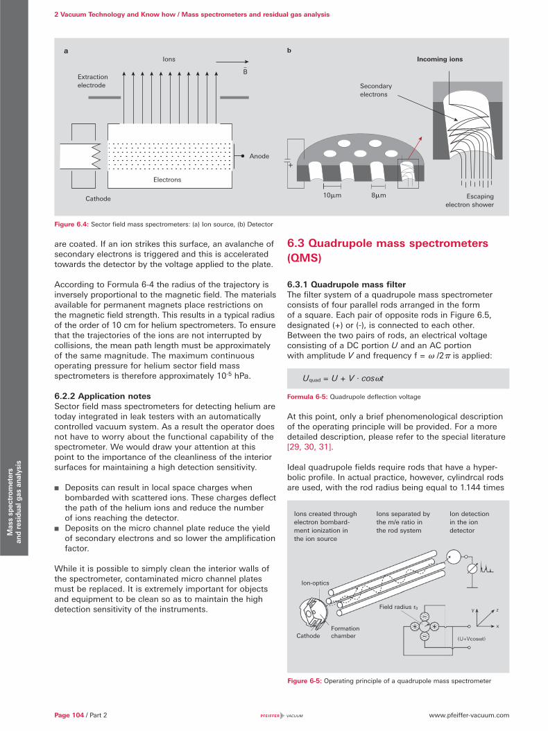
www.pfeiffer-vacuum.comPage 104 / Part 2
2 Vacuum Technology and Know how / Mass spectrometers and residual gas analysisM
ass
spec
trom
eter
s an
d re
sidu
al g
as a
naly
sis
are coated. If an ion strikes this surface, an avalanche of secondary electrons is triggered and this is accelerated towards the detector by the voltage applied to the plate.
According to Formula 6-4 the radius of the trajectory is inversely proportional to the magnetic field. The materials available for permanent magnets place restrictions on the magnetic field strength. This results in a typical radius of the order of 10 cm for helium spectrometers. To ensure that the trajectories of the ions are not interrupted by collisions, the mean path length must be approximately of the same magnitude. The maximum continuous operating pressure for helium sector field mass spectrometers is therefore approximately 10-5 hPa.
6.2.2 Application notesSector field mass spectrometers for detecting helium are today integrated in leak testers with an automatically controlled vacuum system. As a result the operator does not have to worry about the functional capability of the spectrometer. We would draw your attention at this point to the importance of the cleanliness of the interior surfaces for maintaining a high detection sensitivity.
Deposits can result in local space charges when bombarded with scattered ions. These charges deflect the path of the helium ions and reduce the number of ions reaching the detector.
Deposits on the micro channel plate reduce the yield of secondary electrons and so lower the amplification factor.
While it is possible to simply clean the interior walls of the spectrometer, contaminated micro channel plates must be replaced. It is extremely important for objects and equipment to be clean so as to maintain the high detection sensitivity of the instruments.
6.3 Quadrupole mass spectrometers (QMS)
6.3.1 Quadrupole mass filterThe filter system of a quadrupole mass spectrometer consists of four parallel rods arranged in the form of a square. Each pair of opposite rods in Figure 6.5, designated (+) or (-), is connected to each other. Between the two pairs of rods, an electrical voltage consisting of a DC portion U and an AC portion with amplitude V and frequency f = � /2� is applied:
Formula 6-5: Quadrupole deflection voltage
At this point, only a brief phenomenological description of the operating principle will be provided. For a more detailed description, please refer to the special literature [29, 30, 31].
Ideal quadrupole fields require rods that have a hyper-bolic profile. In actual practice, however, cylindrcal rods are used, with the rod radius being equal to 1.144 times
Figure 6.4: Sector field mass spectrometers: (a) Ion source, (b) Detector
Uquad = U + V · cos�t
Figure 6-5: Operating principle of a quadrupole mass spectrometer
Extraction electrode
Cathode
Electrons
Ions
Anode
B
Incoming ions
Escaping electron shower
Secondaryelectrons
10�m 8�m
a b
Ions created throughelectron bombard-ment ionization in the ion source
Ions separated by the m/e ratio in the rod system
Ion detectionin the ion detector
Field radius r0
Ion-optics
Formation chamberCathode
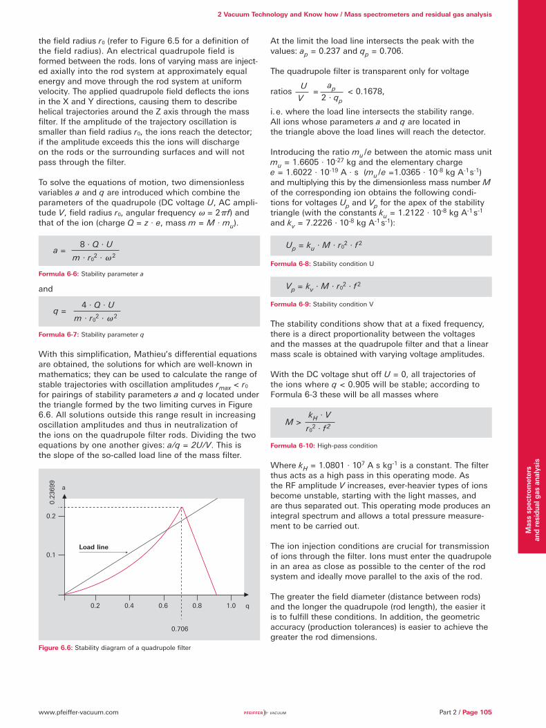
www.pfeiffer-vacuum.com Part 2 / Page 105
2 Vacuum Technology and Know how / Mass spectrometers and residual gas analysis
Mas
s sp
ectr
omet
ers
an
d re
sidu
al g
as a
naly
sis
the field radius r0 (refer to Figure 6.5 for a definition of the field radius). An electrical quadrupole field is formed between the rods. Ions of varying mass are inject-ed axially into the rod system at approximately equal energy and move through the rod system at uniform velocity. The applied quadrupole field deflects the ions in the X and Y directions, causing them to describe helical trajectories around the Z axis through the mass filter. If the amplitude of the trajectory oscillation is smaller than field radius r0, the ions reach the detector; if the amplitude exceeds this the ions will discharge on the rods or the surrounding surfaces and will not pass through the filter.
To solve the equations of motion, two dimensionless variables a and q are introduced which combine the parameters of the quadrupole (DC voltage U, AC ampli-tude V, field radius r0, angular frequency � = 2� f) and that of the ion (charge Q = z · e, mass m = M · mu).
Formula 6-6: Stability parameter a
and
Formula 6-7: Stability parameter q
With this simplification, Mathieu’s differential equations are obtained, the solutions for which are well-known in mathematics; they can be used to calculate the range of stable trajectories with oscillation amplitudes rmax < r0 for pairings of stability parameters a and q located under the triangle formed by the two limiting curves in Figure 6.6. All solutions outside this range result in increasing oscillation amplitudes and thus in neutralization of the ions on the quadrupole filter rods. Dividing the two equations by one another gives: a/q = 2U/V. This is the slope of the so-called load line of the mass filter.
Figure 6.6: Stability diagram of a quadrupole filter
At the limit the load line intersects the peak with the values: ap = 0.237 and qp = 0.706.
The quadrupole filter is transparent only for voltage
ratios = < 0.1678,
i. e. where the load line intersects the stability range. All ions whose parameters a and q are located in the triangle above the load lines will reach the detector.
Introducing the ratio mu / e between the atomic mass unit mu = 1.6605 · 10-27 kg and the elementary charge e = 1.6022 · 10-19 A · s (mu / e =1.0365 · 10-8 kg A-1 s-1) and multiplying this by the dimensionless mass number M of the corresponding ion obtains the following condi-tions for voltages Up and Vp for the apex of the stability triangle (with the constants ku = 1.2122 · 10-8 kg A-1 s-1 and kv = 7.2226 · 10-8 kg A-1 s-1):
Formula 6-8: Stability condition U
Formula 6-9: Stability condition V
The stability conditions show that at a fixed frequency, there is a direct proportionality between the voltages and the masses at the quadrupole filter and that a linear mass scale is obtained with varying voltage amplitudes.
With the DC voltage shut off U = 0, all trajectories of the ions where q < 0.905 will be stable; according to Formula 6-3 these will be all masses where
Formula 6-10: High-pass condition
Where kH = 1.0801 · 107 A s kg-1 is a constant. The filter thus acts as a high pass in this operating mode. As the RF amplitude V increases, ever-heavier types of ions become unstable, starting with the light masses, and are thus separated out. This operating mode produces an integral spectrum and allows a total pressure measure-ment to be carried out.
The ion injection conditions are crucial for transmission of ions through the filter. Ions must enter the quadrupole in an area as close as possible to the center of the rod system and ideally move parallel to the axis of the rod.
The greater the field diameter (distance between rods) and the longer the quadrupole (rod length), the easier it is to fulfill these conditions. In addition, the geometric accuracy (production tolerances) is easier to achieve the greater the rod dimensions.
a = 8 · Q · U
m · r02 · � 2
q = 4 · Q · U
m · r02 · � 2
Up = ku · M · r02 · f 2
Vp = kv · M · r02 · f 2
M > kH · V
r02 · f 2
0.2 0.4 0.6 0.8 1.0
0.2
3699
0.706
q
Load line
0.2
0.1
a
U
V
ap
2 · qp
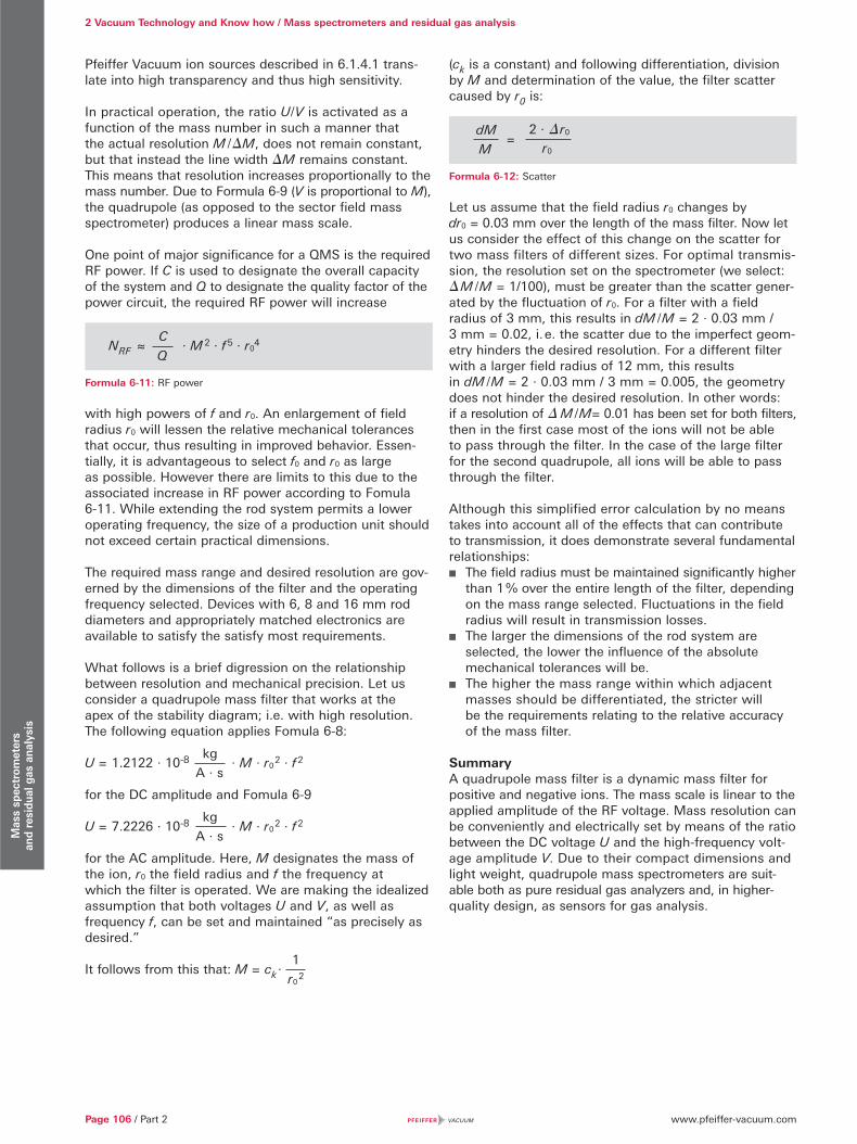
www.pfeiffer-vacuum.comPage 106 / Part 2
2 Vacuum Technology and Know how / Mass spectrometers and residual gas analysisM
ass
spec
trom
eter
s
and
resi
dual
gas
ana
lysi
s
Pfeiffer Vacuum ion sources described in 6.1.4.1 trans-late into high transparency and thus high sensitivity.
In practical operation, the ratio U/V is activated as a function of the mass number in such a manner that the actual resolution M /�M, does not remain constant, but that instead the line width �M remains constant. This means that resolution increases proportionally to the mass number. Due to Formula 6-9 (V is proportional to M), the quadrupole (as opposed to the sector field mass spectrometer) produces a linear mass scale.
One point of major significance for a QMS is the required RF power. If C is used to designate the overall capacity of the system and Q to designate the quality factor of the power circuit, the required RF power will increase
Formula 6-11: RF power
with high powers of f and r0. An enlargement of field radius r0 will lessen the relative mechanical tolerances that occur, thus resulting in improved behavior. Essen-tially, it is advantageous to select f0 and r0 as large as possible. However there are limits to this due to the associated increase in RF power according to Fomula 6-11. While extending the rod system permits a lower operating frequency, the size of a production unit should not exceed certain practical dimensions.
The required mass range and desired resolution are gov-erned by the dimensions of the filter and the operating frequency selected. Devices with 6, 8 and 16 mm rod diameters and appropriately matched electronics are available to satisfy the satisfy most requirements.
What follows is a brief digression on the relationship between resolution and mechanical precision. Let us consider a quadrupole mass filter that works at the apex of the stability diagram; i.e. with high resolution. The following equation applies Fomula 6-8:
U = 1.2122 · 10-8 · M · r0 2 · f 2
for the DC amplitude and Fomula 6-9
U = 7.2226 · 10-8 · M · r0 2 · f 2
for the AC amplitude. Here, M designates the mass of the ion, r0 the field radius and f the frequency at which the filter is operated. We are making the idealized assumption that both voltages U and V, as well as frequency f, can be set and maintained “as precisely as desired.”
It follows from this that: M = ck ·
(ck is a constant) and following differentiation, division by M and determination of the value, the filter scatter caused by r0 is:
Formula 6-12: Scatter
Let us assume that the field radius r0 changes by dr0 = 0.03 mm over the length of the mass filter. Now let us consider the effect of this change on the scatter for two mass filters of different sizes. For optimal transmis-sion, the resolution set on the spectrometer (we select: � M /M = 1/100), must be greater than the scatter gener-ated by the fluctuation of r0. For a filter with a field radius of 3 mm, this results in dM /M = 2 · 0.03 mm / 3 mm = 0.02, i. e. the scatter due to the imperfect geom-etry hinders the desired resolution. For a different filter with a larger field radius of 12 mm, this results in dM /M = 2 · 0.03 mm / 3 mm = 0.005, the geometry does not hinder the desired resolution. In other words: if a resolution of � M /M= 0.01 has been set for both filters, then in the first case most of the ions will not be able to pass through the filter. In the case of the large filter for the second quadrupole, all ions will be able to pass through the filter.
Although this simplified error calculation by no means takes into account all of the effects that can contribute to transmission, it does demonstrate several fundamental relationships:
The field radius must be maintained significantly higher than 1 % over the entire length of the filter, depending on the mass range selected. Fluctuations in the field radius will result in transmission losses.
The larger the dimensions of the rod system are selected, the lower the influence of the absolute mechanical tolerances will be.
The higher the mass range within which adjacent masses should be differentiated, the stricter will be the requirements relating to the relative accuracy of the mass filter.
SummaryA quadrupole mass filter is a dynamic mass filter for positive and negative ions. The mass scale is linear to the applied amplitude of the RF voltage. Mass resolution can be conveniently and electrically set by means of the ratio between the DC voltage U and the high-frequency volt-age amplitude V. Due to their compact dimensions and light weight, quadrupole mass spectrometers are suit-able both as pure residual gas analyzers and, in higher-quality design, as sensors for gas analysis.
NRF ≈ · M 2 · f 5 · r0
4C
Q
=dM
M
2 · � r0
r0
kg
A · s
kg
A · s
1
r0 2

www.pfeiffer-vacuum.com Part 2 / Page 107
2 Vacuum Technology and Know how / Mass spectrometers and residual gas analysis
Mas
s sp
ectr
omet
ers
and
resi
dual
gas
ana
lysi
s
6.3.2 Ion sourcesBefore gases can be analyzed in a mass filter, they must first be ionized in an ion source by means of electron bombardment (Figure 6.6). Electrons are emitted from an electrically heated cathode (filament). A voltage is applied between anode and cathode, which accelerates the electrons. Neutral gas molecules that are present in the formation space between the anode and cathode are ionized by collisions between electrons, forming single and multiple positive ions. The energy of the colliding electrons exerts a significant influence on both the number and type of ions that will be formed.
Figure 6.6: Section through an axial ion source.
Ionization of the neutral particles commences at a minimum electron energy of between 10 and 30 eV (appearance potential). The number of formed ions quickly increases as electron energy rises (acceleration voltage), reaches a maximum at 50 to 150 eV depending upon the type of gas in question, and slowly declines again as energy continues to rise. Since the yield in ions, and thus the sensitivity of the mass spectrometer, should be as large as possible, electron energies between 70 and 100 eV are typically used.
Figure 6.7: Ionization as a function of electron energy
The ion current IK+ of a gas component K can be calculated from the following relationship:
Formula 6-13: Ion current
Where:i_ = electron current (emission current), in Ale = mean path length of the electrons, in cms = differential ionization effect cross section of K,
in 1/(cm · hPa)pK = partial pressure of the gas component K, in hPa
Many types of ions are formed when ionizing complex molecules. In addition to single- and multiple-charge molecule ions (ABC+, ABC++) fragment ions also occur:
ABC+ 2e-
ABC++ + 3e-
AB+ + C + 2e-
BC+ + A + 2e-
A+ + BC + 2e-
C+ + AB + 2e-
B+ + A + C + 2e-
In addition to these types, it is also possible for recombi-nation ions, such as AC+, to form. The occurrence and relative frequency of individual types of ions are charac-teristic of a certain type of molecule and serve as an important aid in identifying the molecule, and thus as an aid in qualitative gas analysis. Figure 6.8 shows the fragment ion distribution (cracking pattern or fragment pattern) of the simple molecule CO2, recorded at 70 eV of electron energy.
Selection of the ion source and the optimal filament material is based upon the requirements imposed by the measurement task. Applications often impose con-tradictory requirements on the ion source. In order to achieve optimal results, the ion source must be matched to the task in hand. This has resulted in the development of different types of ion sources that can almost all be equipped with cathodes made of rhenium (Re), tungsten
lK+ = i– · le · s · pK
1
2
3
4
5
1) Cathode2) Wehnelt electrode3) Anode4) Formation area5) Extraction orifice
100 %5
105
15
0.15
0.01
Relative intensity
Mass number
10 15 20 25 30 35 40 45 amu
CO2
Figure 6.8: Fragment ion distribution of CO2
Pressure indicated
Electron energy [eV]
Ions [cm-1hPa-1]
101
1
10-1
10-2
101 102 103 104 105 106

www.pfeiffer-vacuum.comPage 108 / Part 2
2 Vacuum Technology and Know how / Mass spectrometers and residual gas analysisM
ass
spec
trom
eter
s an
d re
sidu
al g
as a
naly
sis
or yttriated iridium (Y2O3 / Ir). Tungsten (W) cathodes are preferred in the UHV range or where the vapor pressure of rhenium (Re) could have a disturbing effect. However the brittleness of tungsten cathodes due to the tungsten/carbon/oxygen cycle must be taken into account; i.e. due to the formation of W2C. Yttriated iridium is increasingly used today instead of the pure metal cathodes that were used in the past. The advantages offered by these cath-odes are significantly lower operating temperature and relative insensitivity to air inrush. Consequently, the preferred fields of implementation for these cathodes are the analysis of temperature-sensitive substances, e.g. metal-organic compounds, or the analysis of contami-nants in gas mixtures containing a high concentration of oxygen.
The various ion sources are described below on the basis of their attributes and fields of application. What all ion sources have in common is that they can be connected to a potential of up to 150 V. This avoids signal background due to EID ions ( EID = Electron Impact Desorption, also known as: ESD = Electron Stimulated Desorption). This technology will be explained in detail later.
Axial ion sourceThis ion source is characterized by its extremely robust mechanical design and high sensitivity. It is primarily employed for residual gas analysis in high vacuum sys-tems due to its open construction. Figure 6.6 shows a schematic diagram of an axial ion source. The cathode (1) is arranged within a hole in the Wehnelt electrode (2) and is connected with this electrode on one side. The electrons accelerated toward the anode (3) ionize gas molecules in the formation area (4). The positive ions reach the mass filter through the extraction orifice (5). Due to its relatively open construction, only minor falsification occurs through desorption and surface reactions.
Grid ion source
Figure 6.9: Grid ion source
A grid ion source is used to examine residual gas in UHV or even XHV applications. Its extremely open construction and the choice of materials ensure very low internal gas emissions. This ion source is equipped with two tungsten filaments that can be heated simulta-neously for degassing. If work is to be performed at pressures below 10 -11 hPa, rod systems that have been highly degassed especially for this purpose should be used. Measurements in the pressure range below 10-10 hPa can be falsified by so-called EID (electron impact desorption) ions. [32]. These (H+, O+, F+, Cl+) ions are directly desorbed by electron bombardment of surfaces, often with a high yield. EID ions come from adsorbed coatings that originate earlier in the history of the UHV equipment or the ion source, and usually have an initial energy of several eV. This attribute is utilized by careful selection of the field axis voltage to suppress the EID ions relative to ions from the gas phase with an energy of approximately 100 eV (Figure 6.10).
Table 6.1: Filament materials and their use
1) Grid
2) Filaments
1
2
Material Temperature Applicable gases Remarks
Y2 O3 / lr 1,300 °C Inert gases, air / O2,NOx, SOx
Short service life with halogens, insensitive to high O2 concentrations, generates some CO / CO2 from O2 or H2O background
W 1,800 °C Inert gases, H2, halogens, freons
Short service life with O2 applications,generates some CO / CO2, from O2 or H2O background, C causes brittleness
Re 1,800 °C Inert gases,hydrocarbons, H2,halogens, freons
Service life around three months due to vaporization of the material, used with hydrocarbons
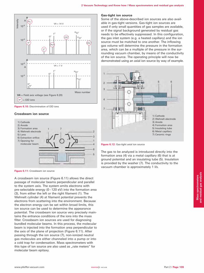
www.pfeiffer-vacuum.com Part 2 / Page 109
2 Vacuum Technology and Know how / Mass spectrometers and residual gas analysis
Mas
s sp
ectr
omet
ers
and
resi
dual
gas
ana
lysi
s
Figure 6.10: Discrimination of EID ions
Crossbeam ion source
Figure 6.11: Crossbeam ion source
A cross beam ion source (Figure 6.11) allows the direct passage of molecular beams perpendicular and parallel to the system axis. The system emits electrons with pre-selectable energy (0 – 120 eV) into the formation area (3), from either the left or the right filament (1). The Wehnelt cylinder (4) at filament potential prevents the electrons from scattering into the environment. Because the electron energy can be set within broad limits, this ion source can be used to determine the appearance potential. The crossbeam ion source very precisely main-tains the entrance conditions of the ions into the mass filter. Crossbeam ion sources are used for diagnosing bundled molecular beams. In this process, the molecular beam is injected into the formation area perpendicular to the axis of the plane of projection (Figure 6.11). After passing through the ion source (7), non-ionized neutral gas molecules are either channeled into a pump or into a cold trap for condensation. Mass spectrometers with this type of ion source are also used as „rate meters“ for molecular beam epitaxy.
Gas-tight ion source Some of the above-described ion sources are also avail-able in gas-tight versions. Gas-tight ion sources are used if only small quantities of gas samples are available, or if the signal background generated by residual gas needs to be effectively suppressed. In this configuration, the gas inlet system (e.g. a heated capillary) and the ion source must be matched to one another. The inflowing gas volume will determine the pressure in the formation area, which can be a multiple of the pressure in the sur-rounding vacuum chamber, by means of the conductivity of the ion source. The operating principle will now be demonstrated using an axial ion source by way of example.
Figure 6.12: Gas-tight axial ion source
The gas to be analyz ed is introduced directly into the formation area (4) via a metal capillary (6) that is at ground potential and an insulating tube (5). Insulation is provided by the washer (7). The conductivity to the vacuum chamber is approximately 1 l/s.
V4 = 1 V
V4 = 14 V
Mass number
Inte
nsi
ty
10-8
10-8
10-9
10-9
A
A
C+
O+F+
CO+
H2+
H+
H2O
35Cl+
37Cl+
CO2+
H+
H+
O+F+
35Cl+
37Cl+
H+ = EID ions
V4 = Field axis voltage (see Figure 6.20)
1) Cathode2) Anode3) Formation area4) Wehnelt electrode5) Lens 6) Extraction orifice7) Opening for
molecular beam
1 72
3
1
4
6
5
1) Cathode 2) Wehnelt electrode 3) Anode 4) Formation area5) Insulating tube6) Metal capillary7) Ceramic rings
1
2
3
4
7
5 6

www.pfeiffer-vacuum.comPage 110 / Part 2
2 Vacuum Technology and Know how / Mass spectrometers and residual gas analysisM
ass
spec
trom
eter
s an
d re
sidu
al g
as a
naly
sis
Sputter process monitor (SPM) ion sourceIn this ion source, the formation area (7) is connected directly with the process chamber. The analyzer is equipped with a small turbopumping station (1), which also evacuates the cathode space (5) to approximately 10-5 hPa. Electrons are injected into the formation area (7) from the low pressure side through small holes in order to ionize the gas. The ions thus formed are extracted to the mass filter through a small opening to the low-pressure side. This ion source offers two crucial advan-tages for examining the composition of the gas in sputtering processes. On one hand, the analysis is per-formed at an ion source pressure that is up to three orders of magnitude higher; i.e. a higher process pressure can be tolerated in the vacuum chamber. On the other hand, the hot filament is not in direct contact with the sputtering process. This avoids contamination by the hot cathode during sensitive processes.
Standard PrismaPlus ion sourceThe PrismaPlus mass spectrometer from Pfeiffer Vacuum is equipped with this robust and highly sensitive ion source. It is an ion source that is especially suited for residual gas analysis. Its design is comparable to that
of a grid source, with two cathodes, resulting in reliable operation. Both an open version as well as a gas-tight version with gas inlet in the axial direction are available.
All ion sources described here ionize by means of electron impact. The ion sources can be categorized into two groups:
Open ion sources are used if the gas to be analyzed is at high vacuum < 1 · 10-4 hPa.
Closed ion sources are used in analytical applications, for example, where only small volumes of sample gas are available or to reduce background effects of the mass spectrometer vacuum system.
Closed ion sources are used in combination with a differentially pumped system (Figure 6.13) in order to analyze higher-pressure gases.
6.3.3 DetectorsThe ions that are separated in the rod system on the basis of their mass-to-charge ratio can be electrically detected with various types of detectors:
By means of a Faraday cup for direct measurement of the ion current using an electrometer amplifier
Using a secondary electron multiplier (SEM) of discrete design with individual dynodes
By means of a continuous secondary electron multiplier (C-SEM)
Detector selection will primarily be based upon require-ments that relate to detection sensitivity, detection speed and signal-to-noise ratio. However it will also be governed by other application-specific requirements that relate to stability, thermal and chemical resistance, as well as space requirements.
Faraday cupIn the simplest case, the ions strike a Faraday collector (Faraday cup), where they give up their electrical charge.
Figure 6.15: Operating principle of a Faraday Cup
The resulting current is converted to a voltage that is proportional to the ion current by means of a sensitive current-to-voltage converter (electrometer amplifier). The sensitivity of the electrometer amplifier with the Faraday cup is typically in the order of K = 10-4 A/hPa. The input resistance R of the current amplifier needs to be extremely high. With typical wiring capacities C this results in time constants � = R · C in the range 0.1 s < � < 100 s. Depending upon the time constant, the measurement limit is between 1 · 10-16 and 1 · 10-14 A, and so minimal partial pressures in the order of pmin = 10-10 hPa can be detected. For UHV systems with total pressures of under 10-8 hPa this is usually.
Process chamber10-2 hPa
SPMIon source
10-5 hPa
7
6 5 4
23
1
1) Turbomolecular pump for differential pumping2) Secondary electron multiplier (SEM)3) Deflection unit 4) Quadrupole mass filter5) Filaments 6) High-conductivity piping to process chamber7) Formation area
Gas-tight designOpen design
Figure 6.13: SPM ion source
Figure 6.14: PrismaPlus ion sources
= Selected positively charged ions
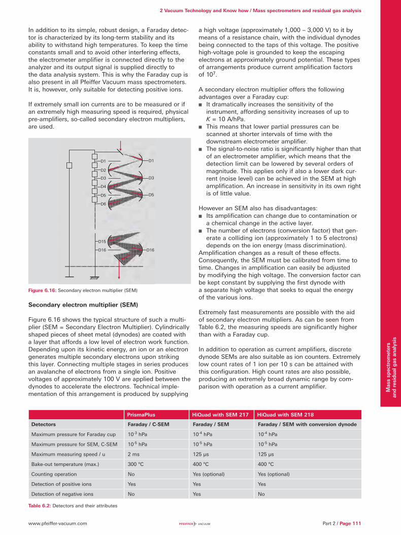
www.pfeiffer-vacuum.com Part 2 / Page 111
2 Vacuum Technology and Know how / Mass spectrometers and residual gas analysis
Mas
s sp
ectr
omet
ers
and
resi
dual
gas
ana
lysi
s
In addition to its simple, robust design, a Faraday detec-tor is characterized by its long-term stability and its ability to withstand high temperatures. To keep the time constants small and to avoid other interfering effects, the electrometer amplifier is connected directly to the analyzer and its output signal is supplied directly to the data analysis system. This is why the Faraday cup is also present in all Pfeiffer Vacuum mass spectrometers. It is, however, only suitable for detecting positive ions.
If extremely small ion currents are to be measured or if an extremely high measuring speed is required, physical pre-amplifiers, so-called secondary electron multipliers, are used.
Figure 6.16: Secondary electron multiplier (SEM)
Secondary electron multiplier (SEM)
Figure 6.16 shows the typical struc ture of such a multi-plier (SEM = Secondary Electron Multiplier). Cylindrically shaped pieces of sheet metal (dynodes) are coated with a layer that affords a low level of electron work function. Depending upon its kinetic energy, an ion or an electron generates multiple secondary electrons upon striking this layer. Connecting multiple stages in series produces an avalanche of electrons from a single ion. Positive voltages of approximately 100 V are applied between the dynodes to accelerate the electrons. Technical imple-mentation of this arrangement is produced by supplying
a high voltage (approximately 1,000 – 3,000 V) to it by means of a resistance chain, with the individual dynodes being connected to the taps of this voltage. The positive high-voltage pole is grounded to keep the escaping electrons at approximately ground potential. These types of arrangements produce current amplification factors of 107.
A secondary electron multiplier offers the following advantages over a Faraday cup:
It dramatically increases the sensitivity of the instrument, affording sensitivity increases of up to K = 10 A/hPa.
This means that lower partial pressures can be scanned at shorter intervals of time with the downstream electrometer amplifier.
The signal-to-noise ratio is significantly higher than that of an electrometer amplifier, which means that the detection limit can be lowered by several orders of magnitude. This applies only if also a lower dark cur-rent (noise level) can be achieved in the SEM at high amplification. An increase in sensitivity in its own right is of little value.
However an SEM also has disadvantages: Its amplification can change due to contamination or
a chemical change in the active layer. The number of electrons (conversion factor) that gen-
erate a colliding ion (approximately 1 to 5 electrons) depends on the ion energy (mass discrimination).
Amplification changes as a result of these effects. Consequently, the SEM must be calibrated from time to time. Changes in amplification can easily be adjusted by modifying the high voltage. The conversion factor can be kept constant by supplying the first dynode with a separate high voltage that seeks to equal the energy of the various ions.
Extremely fast measurements are possible with the aid of secondary electron multipliers. As can be seen from Table 6.2, the measuring speeds are significantly higher than with a Faraday cup.
In addition to operation as current amplifiers, discrete dynode SEMs are also suitable as ion counters. Extremely low count rates of 1 ion per 10 s can be attained with this configuration. High count rates are also possible, producing an extremely broad dynamic range by com-parison with operation as a current amplifier.
PrismaPlus HiQuad with SEM 217 HiQuad with SEM 218
Detectors Faraday / C-SEM Faraday / SEM Faraday / SEM with conversion dynode
Maximum pressure for Faraday cup 10-3 hPa 10-4 hPa 10-4 hPa
Maximum pressure for SEM, C-SEM 10-5 hPa 10-5 hPa 10-5 hPa
Maximum measuring speed / u 2 ms 125 μs 125 μs
Bake-out temperature (max.) 300 °C 400 °C 400 °C
Counting operation No Yes (optional) Yes (optional)
Detection of positive ions Yes Yes Yes
Detection of negative ions No Yes No
—.—
.—.—
.—.
—.—.—.—.—.—.—.—.—.—.—.—.—.—
D1
D2
D3
D4
D5
D6
D5
D3
D1
D15
D16 D16
Table 6.2: Detectors and their attributes

www.pfeiffer-vacuum.comPage 112 / Part 2
2 Vacuum Technology and Know how / Mass spectrometers and residual gas analysisM
ass
spec
trom
eter
s
and
resi
dual
gas
ana
lysi
s
In the counting mode, the speed of the SEM defines the upper limit of the dynamic range. With a pulse width of 20 ns, non-linearity begins at a count rate of 106 events per second. Given its pulse width, the SEM must be suit-able as a counter.
What all secondary electron multipliers have in common is that they are restricted to operating at pressures of less than 10-5 hPa. At higher pressures than these, the layer of water on the dynodes can lead to pyrolysis in operation, and thus to premature aging. Due to the high voltages involved, gas discharges that could destroy the SEM can occur at high pressures of p > 10-5 hPa.
Continuous secondary electron multiplier (C-SEM)A C-SEM (Figure 6.17) consists of a glass tube whose interior is coated with a conductive layer that has high resistance and a low work function. High voltage is applied to the layer in order to obtain a uniform voltage gradient throughout the length of the tube. Ions from the quadrupole system are routed to the conversion dynode and generate secondary electrons that trigger an elec-tron avalanche in the tube. Current amplification factors of 106 are attained at an amplification voltage of 2,500 V.
Figure 6.17: Operating principle of continuous secondary electron multiplier (C-SEM)
Here, too, amplification and dark current govern the signal-to-noise ratio, and the maximum current / dark current ratio of 106 is the current amplification factor. Thanks to a C-SEM arrangement that is slightly offset relative to the axis of the quadrupole, both a Faraday cup as well as a C-SEM can be used next to one another in the analyzer, with changeover from one detector to the other being possible when necessary.
6.3.4 Vacuum systemsThe ions must be able to pass through the quadrupole filter without colliding with neutral gas particles. Mean path lengths which are attained at pressures p < 10-4 hPa are required for the operation of quadrupole mass spectrometers. This necessitates an appropriate pumping station with pressure monitoring. In order to perform gas analysis with optimal sensitivity, not only a low base pressure is necessary but the residual gas should contain only unavoidable partial pressures stem-ming from desorption from the walls of the equipment. Residual gas spectra of this type and low base pressures are best attained with turbo drag pumping stations (Figure 4.27). An additional total pressure gauge protects the mass spectrometer against being energized at exces-sively high pressures. When setting up such a system, attention must be paid to an appropriate arrangement of gas inlet, valves, pumps and measurement instruments in order to avoid falsification stemming from unfavorable flow conditions. A separate pumping station that evacu-ates the measurement system is often required during the course of vacuum processes that run at high pressure. Small pumping stations with turbo drag pumps and dia-phragm pumps are used for this purpose.
6.3.5 Inlet systemsGases to be analyzed must usually be reduced from atmospheric pressure to pressures of less than the working pressure of the mass spectrometer (MS). Many vacuum technology processes that are monitored by mass spectrometers occur in pressure ranges p > 10-4 hPa. An essential element of a quadrupole mass spectrometer is therefore a suitable gas inlet system for the particular application. Various pressure reducing procedures are used, depending on the pressure gradi-ent in question.
Gas mixtures should be admitted to the mass spectro-meter without de-mixing if possible:
At pressures p > 10 hPa, pressure is reduced by means of a (heatable) capillary, in which laminar flow prevails, with a downstream gas inlet valve. Under some circumstances, pressure reduction by means of an additional pump will be necessary.
At pressures p < 10 hPa, pressure is reduced with an orifice and a mass spectrometer which is differentially pumped with a turbomolecular pump.
At pressures p < 10-4 hPa the mass spectrometer can be installed directly in the process chamber with an open ion source.
Where an orifice is used for reducing pressure, its gas-type dependent conductivity is canceled out by the equally gas-type dependent conductivity of the flow path towards the pump, which means that the concentrations in the QMS reflect the true gas composition.
Ion+
Conversion dynodee-
Output voltage U
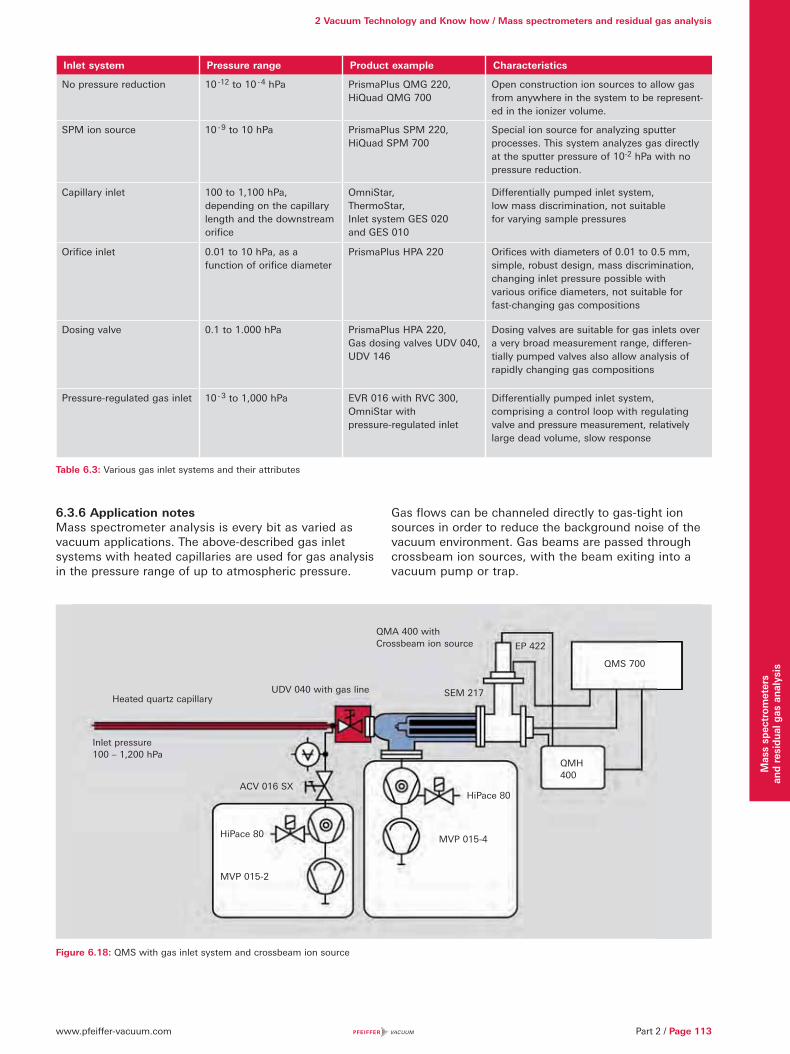
www.pfeiffer-vacuum.com Part 2 / Page 113
2 Vacuum Technology and Know how / Mass spectrometers and residual gas analysis
Mas
s sp
ectr
omet
ers
and
resi
dual
gas
ana
lysi
s
Table 6.3: Various gas inlet systems and their attributes
6.3.6 Application notesMass spectrometer analysis is every bit as varied as vacuum applications. The above-described gas inlet systems with heated capillaries are used for gas analysis in the pressure range of up to atmospheric pressure.
Gas flows can be channeled directly to gas-tight ion sources in order to reduce the background noise of the vacuum environment. Gas beams are passed through crossbeam ion sources, with the beam exiting into a vacuum pump or trap.
Inlet system Pressure range Product example Characteristics
No pressure reduction 10 -12 to 10 - 4 hPa PrismaPlus QMG 220, HiQuad QMG 700
Open construction ion sources to allow gas from anywhere in the system to be represent-ed in the ionizer volume.
SPM ion source 10 - 9 to 10 hPa PrismaPlus SPM 220,HiQuad SPM 700
Special ion source for analyzing sputter processes. This system analyzes gas directly at the sputter pressure of 10-2 hPa with no pressure reduction.
Capillary inlet 100 to 1,100 hPa, depending on the capillarylength and the downstreamorifice
OmniStar,ThermoStar,Inlet system GES 020 and GES 010
Differentially pumped inlet system, low mass discrimination, not suitable for varying sample pressures
Orifice inlet 0.01 to 10 hPa, as a function of orifice diameter
PrismaPlus HPA 220 Orifices with diameters of 0.01 to 0.5 mm, simple, robust design, mass discrimination, changing inlet pressure possible with various orifice diameters, not suitable for fast-changing gas compositions
Dosing valve 0.1 to 1.000 hPa PrismaPlus HPA 220,Gas dosing valves UDV 040, UDV 146
Dosing valves are suitable for gas inlets over a very broad measurement range, differen-tially pumped valves also allow analysis of rapidly changing gas compositions
Pressure-regulated gas inlet 10 - 3 to 1,000 hPa EVR 016 with RVC 300,OmniStar with pressure-regulated inlet
Differentially pumped inlet system, comprising a control loop with regulating valve and pressure measurement, relatively large dead volume, slow response
HiPace 80
MVP 015-4
QMH400
QMS 700
EP 422
SEM 217
HiPace 80
MVP 015-2
ACV 016 SX
UDV 040 with gas lineHeated quartz capillary
Inlet pressure100 – 1,200 hPa
QMA 400 withCrossbeam ion source
Figure 6.18: QMS with gas inlet system and crossbeam ion source

www.pfeiffer-vacuum.comPage 114 / Part 2
2 Vacuum Technology and Know how / Mass spectrometers and residual gas analysisM
ass
spec
trom
eter
s an
d re
sidu
al g
as a
naly
sis
In the pressure range p < 10 hPa (etching, sputtering or other coating processes), the gas is admitted into the mass spectrometer via an orifice or a valve. A turbopump is attached to the measuring system for pressure reduction. There are special versions for corrosive gases.
At extremely low pressures, particularly in the UHV range, open ion sources are used which have a particularly small surface area and therefore low outgassing rates (grid ion source). Due to the low gas densities, secondary electron multipliers (SEM) that are arranged perpendicular to the axis of the quadrupole must be used as detectors. To improve the signal-to-noise ratio, a turbopump that pumps down the inflowing neutral particles is attached opposite the SEM.
Secondary ion mass spectrometry (SIMS) represents a special case. In this process, ions are shot onto surfaces that in turn release positively or negatively charged secondary ions. These are detected directly by a QMS without an ion source. The measuring arrangement described in the preceding section is used in this case as well.
6.4 Portfolio overview
Pfeiffer Vacuum offers two basic mass spectrometer models:
The compact PrismaPlus with a 6 mm diameter rod system and a length of 100 mm, and
The high-resolution HiQuad with mass filter diameters of 8 mm and 16 mm and a length of 300 mm.
PrismaPlusThis is a compact device whose entire electronics are attached to the analyzer and can be removed for bake-out. The PrismaPlus offers the following features:
Mass ranges of 100, 200 and 300 u A Faraday cup and a C-SEM are available as detectors Can be equipped with a variety of ion sources and
filaments The analyzer can be baked out at up to 300°C
The PrismaPlus is used as a standalone device and can also be integrated into modules and analysis systems.
HiQuad These devices offer the utmost in accuracy and possess the following features:
The mass ranges 1–16 u, 1–128 u, 1–340 u, 1–300 u, 1–512 u, 1–1,024 u and 1–2,048 u are covered by differnt models.
There are various mass filters with rod diameters: 6 mm, 8 mm molybdenum, 8 mm stainless steel and 16 mm molybdenum
Figure 6.19: Differentially pumped QMS with various gas inlets
a) 50 hPa > p > 1 · 10- 4 hPa
b) 10 hPa > p > 1 · 10- 7 hPa
c) 10 hPa > p > 1 · 10- 7 hPa
SVV dual valvewith 1 x orifice
HPI 040, manual,with 2 x orifices
UDV 040
p < 1 · 10- 6 hPa
HiPace 80
MVP 015-4
Power supply
PrismaPlusC-SEM open ion source
24 VDC
QUADERA®
Process chamber
LAN interface
Analog and digital interfaces
PKR 251
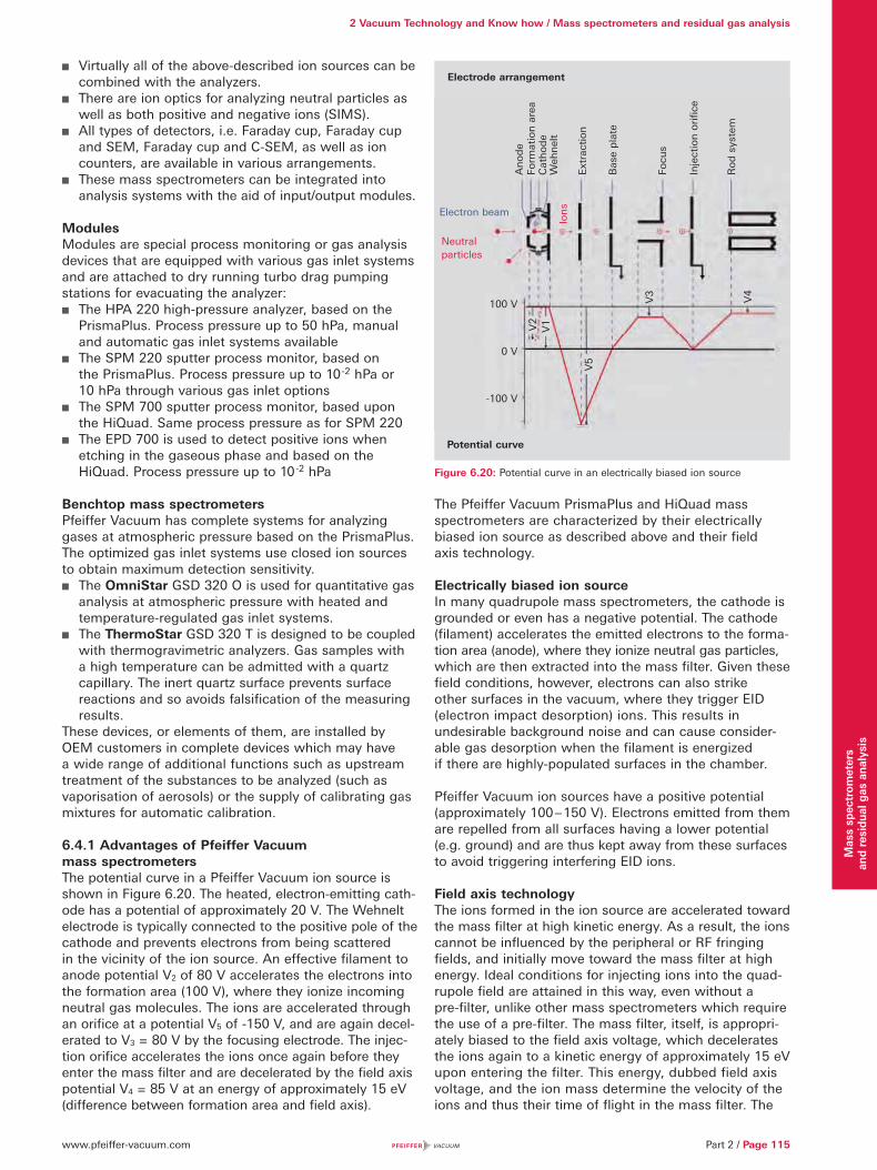
www.pfeiffer-vacuum.com Part 2 / Page 115
2 Vacuum Technology and Know how / Mass spectrometers and residual gas analysis
Mas
s sp
ectr
omet
ers
and
resi
dual
gas
ana
lysi
s
Virtually all of the above-described ion sources can be combined with the analyzers.
There are ion optics for analyzing neutral particles as well as both positive and negative ions (SIMS).
All types of detectors, i.e. Faraday cup, Faraday cup and SEM, Faraday cup and C-SEM, as well as ion counters, are available in various arrangements.
These mass spectrometers can be integrated into analysis systems with the aid of input/output modules.
ModulesModules are special process monitoring or gas analysis devices that are equipped with various gas inlet systems and are attached to dry running turbo drag pumping stations for evacuating the analyzer:
The HPA 220 high-pressure analyzer, based on the PrismaPlus. Process pressure up to 50 hPa, manual and automatic gas inlet systems available
The SPM 220 sputter process monitor, based on the PrismaPlus. Process pressure up to 10-2 hPa or 10 hPa through various gas inlet options
The SPM 700 sputter process monitor, based upon the HiQuad. Same process pressure as for SPM 220
The EPD 700 is used to detect positive ions when etching in the gaseous phase and based on the HiQuad. Process pressure up to 10-2 hPa
Benchtop mass spectrometersPfeiffer Vacuum has complete systems for analyzing gases at atmospheric pressure based on the PrismaPlus. The optimized gas inlet systems use closed ion sources to obtain maximum detection sensitivity.
The OmniStar GSD 320 O is used for quantitative gas analysis at atmospheric pressure with heated and temperature-regulated gas inlet systems.
The ThermoStar GSD 320 T is designed to be coupled with thermogravimetric analyzers. Gas samples with a high temperature can be admitted with a quartz capillary. The inert quartz surface prevents surface reactions and so avoids falsification of the measuring results.
These devices, or elements of them, are installed by OEM customers in complete devices which may have a wide range of additional functions such as upstream treatment of the substances to be analyzed (such as vaporisation of aerosols) or the supply of calibrating gas mixtures for automatic calibration.
6.4.1 Advantages of Pfeiffer Vacuum mass spectrometers The potential curve in a Pfeiffer Vacuum ion source is shown in Figure 6.20. The heated, electron -emitting cath-ode has a potential of approximately 20 V. The Wehnelt electrode is typically connected to the positive pole of the cathode and prevents electrons from being scattered in the vicinity of the ion source. An effective filament to anode potential V2 of 80 V accelerates the electrons into the formation area (100 V), where they ionize incoming neutral gas molecules. The ions are accelerated through an orifice at a potential V5 of -150 V, and are again decel-erated to V3 = 80 V by the focusing electrode. The injec-tion orifice accelerates the ions once again before they enter the mass filter and are decelerated by the field axis potential V4 = 85 V at an energy of approximately 15 eV (difference between formation area and field axis).
Figure 6.20: Potential curve in an electrically biased ion source
The Pfeiffer Vacuum PrismaPlus and HiQuad mass spectrometers are characterized by their electrically biased ion source as described above and their field axis technology.
Electrically biased ion sourceIn many quadrupole mass spectrometers, the cathode is grounded or even has a negative potential. The cathode (filament) accelerates the emitted electrons to the forma-tion area (anode), where they ionize neutral gas particles, which are then extracted into the mass filter. Given these field conditions, however, electrons can also strike other surfaces in the vacuum, where they trigger EID (electron impact desorption) ions. This results in undesirable background noise and can cause consider-able gas desorption when the filament is energized if there are highly-populated surfaces in the chamber.
Pfeiffer Vacuum ion sources have a positive potential (approximately 100 – 150 V). Electrons emitted from them are repelled from all surfaces having a lower potential (e.g. ground) and are thus kept away from these surfaces to avoid triggering interfering EID ions.
Field axis technologyThe ions formed in the ion source are accelerated toward the mass filter at high kinetic energy. As a result, the ions cannot be influenced by the peripheral or RF fringing fields, and initially move toward the mass filter at high energy. Ideal conditions for injecting ions into the quad-rupole field are attained in this way, even without a pre-filter, unlike other mass spectrometers which require the use of a pre-filter. The mass filter, itself, is appropri-ately biased to the field axis voltage, which decelerates the ions again to a kinetic energy of approximately 15 eV upon entering the filter. This energy, dubbed field axis voltage, and the ion mass determine the velocity of the ions and thus their time of flight in the mass filter. The
Electrode arrangement
Potential curve
Electron beam
Neutral particles
An
od
eFo
rmat
ion
are
aC
ath
od
e
Ext
ract
ion
Bas
e p
late
Focu
s
Inje
ctio
n o
rifi
ce
Ro
d s
yste
m
Ion
s
100 V
0 V
-100 V
V2
V1
V5
V3
V4
Weh
nel
t
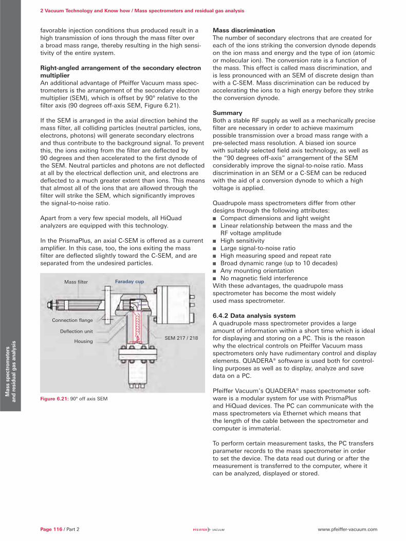
www.pfeiffer-vacuum.comPage 116 / Part 2
2 Vacuum Technology and Know how / Mass spectrometers and residual gas analysisM
ass
spec
trom
eter
s an
d re
sidu
al g
as a
naly
sis
favorable injection conditions thus produced result in a high transmission of ions through the mass filter over a broad mass range, thereby resulting in the high sensi-tivity of the entire system.
Right-angled arrangement of the secondary electron multiplierAn additional advantage of Pfeiffer Vacuum mass spec-trometers is the arrangement of the secondary electron multiplier (SEM), which is offset by 90° relative to the filter axis (90 degrees off-axis SEM, Figure 6.21).
If the SEM is arranged in the axial direction behind the mass filter, all colliding particles (neutral particles, ions, electrons, photons) will generate secondary electrons and thus contribute to the background signal. To prevent this, the ions exiting from the filter are deflected by 90 degrees and then accelerated to the first dynode of the SEM. Neutral particles and photons are not deflected at all by the electrical deflection unit, and electrons are deflected to a much greater extent than ions. This means that almost all of the ions that are allowed through the filter will strike the SEM, which significantly improves the signal-to-noise ratio.
Apart from a very few special models, all HiQuad analyzers are equipped with this technology.
In the PrismaPlus, an axial C-SEM is offered as a current amplifier. In this case, too, the ions exiting the mass filter are deflected slightly toward the C-SEM, and are separated from the undesired particles.
Mass discriminationThe number of secondary electrons that are created for each of the ions striking the conversion dynode depends on the ion mass and energy and the type of ion (atomic or molecular ion). The conversion rate is a function of the mass. This effect is called mass discrimination, and is less pronounced with an SEM of discrete design than with a C-SEM. Mass discrimination can be reduced by accelerating the ions to a high energy before they strike the conversion dynode.
SummaryBoth a stable RF supply as well as a mechanically precise filter are necessary in order to achieve maximum possible transmission over a broad mass range with a pre-selected mass resolution. A biased ion source with suitably selected field axis technology, as well as the “90 degrees off-axis” arrangement of the SEM considerably improve the signal-to-noise ratio. Mass discrimination in an SEM or a C-SEM can be reduced with the aid of a conversion dynode to which a high voltage is applied.
Quadrupole mass spectrometers differ from other designs through the following attributes:
Compact dimensions and light weight Linear relationship between the mass and the
RF voltage amplitude High sensitivity Large signal-to-noise ratio High measuring speed and repeat rate Broad dynamic range (up to 10 decades) Any mounting orientation No magnetic field interference
With these advantages, the quadrupole mass spectrometer has become the most widelyused mass spectrometer.
6.4.2 Data analysis systemA quadrupole mass spectrometer provides a large amount of information within a short time which is ideal for displaying and storing on a PC. This is the reason why the electrical controls on Pfeiffer Vacuum mass spectrometers only have rudimentary control and display elements. QUADERA® software is used both for control-ling purposes as well as to display, analyze and save data on a PC.
Pfeiffer Vacuum’s QUADERA® mass spectrometer soft-ware is a modular system for use with PrismaPlus and HiQuad devices. The PC can communicate with the mass spectrometers via Ethernet which means that the length of the cable between the spectrometer and computer is immaterial.
To perform certain measurement tasks, the PC transfers parameter records to the mass spectrometer in order to set the device. The data read out during or after the measurement is transferred to the computer, where it can be analyzed, displayed or stored.
Mass filter Faraday cup
Connection flange
Deflection unit
HousingSEM 217 / 218
Figure 6.21: 90° off axis SEM
www.pfeiffer-vacuum.com Part 2 / Page 117
2 Vacuum Technology and Know how / Mass spectrometers and residual gas analysis
Mas
s sp
ectr
omet
ers
an
d re
sidu
al g
as a
naly
sis
Typical display formats are: Mass spectra with adjustable mass range, and linearly
or logarithmically scaled axes for the concentration Trend display of the chronological sequence of partial
pressures Bar graph to reduce the quantity of data
Typical measuring tasks, such as residual gas analysis or leak detection, are pre-programmed and can be launched with a mouse click.
If quantitative analysis is to be performed, the mass spectrometer must be calibrated beforehand. If this involves recurring processes, such as calibration with subsequent quantitative analysis, these processes can be programmed with VSTA (Visual Studio Tools for Applications). Programming skills are not required, as pre-engineered modules are available for this purpose.
To solve complicated measurement tasks, a library containing fragment ion distributions for several frequent-ly occurring gases and compounds is available in the QUADERA® software. However these and other distribu-tions obtained from spectra libraries can only be viewed as guideline values, as they are influenced by various parameters, such as ionization energy, temperature or the transmission characteristics of the mass analyzer.
In analyzing mixtures containing multiple gas compo-nents, the problem of overlapping ion currents of differing origin on the same mass numbers is one that frequently occurs. There are mass numbers whose inten-sity is produced exclusively by a single gas component (e. g. argon on mass number 40, oxygen on mass number 32, carbon dioxide on mass number 44 and water on mass number 18).
In the case of other mass numbers, the overall intensity of the detected ion current is governed by the overlapping of various concentrations of fragment ions from different gas components. Depending upon the composition and concentration ratios in the gas mixture to be analyzed, suitable algorithms and calibration procedures must also be formulated for the measurement task in question. Before carrying out quantitative gas analyses by applying suitable calibration gas mixtures that each have non-overlapping components, the calibration factors for each single gas component must be determined for all over-lapping mass numbers. The concentration and/or partial pressure for these gases can then be determined by a matrix calculation. The QUADERA® mass spectrometer software performs the matrix calculation and provides the necessary gas-specific calibration routines.
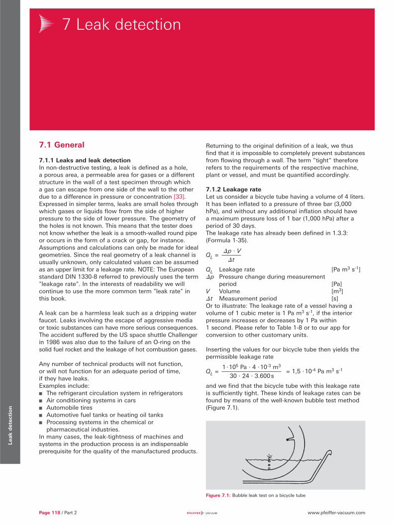
www.pfeiffer-vacuum.comPage 118 / Part 2
Lea
k d
etec
tion
7 Leak detection
7.1 General
7.1.1 Leaks and leak detectionIn non-destructive testing, a leak is defined as a hole, a porous area, a permeable area for gases or a different structure in the wall of a test specimen through which a gas can escape from one side of the wall to the other due to a difference in pressure or concentration [33]. Expressed in simpler terms, leaks are small holes through which gases or liquids flow from the side of higher pressure to the side of lower pressure. The geometry of the holes is not known. This means that the tester does not know whether the leak is a smooth-walled round pipe or occurs in the form of a crack or gap, for instance. Assumptions and calculations can only be made for ideal geometries. Since the real geometry of a leak channel is usually unknown, only calculated values can be assumed as an upper limit for a leakage rate. NOTE: The European standard DIN 1330-8 referred to previously uses the term "leakage rate". In the interests of readability we will continue to use the more common term "leak rate" in this book.
A leak can be a harmless leak such as a dripping water faucet. Leaks involving the escape of aggressive media or toxic substances can have more serious consequences. The accident suffered by the US space shuttle Challenger in 1986 was also due to the failure of an O-ring on the solid fuel rocket and the leakage of hot combustion gases.
Any number of technical products will not function, or will not function for an adequate period of time, if they have leaks. Examples include:
The refrigerant circulation system in refrigerators Air conditioning systems in cars Automobile tires Automotive fuel tanks or heating oil tanks Processing systems in the chemical or
pharmaceutical industries. In many cases, the leak-tightness of machines and systems in the production process is an indispensable prerequisite for the quality of the manufactured products.
Returning to the original definition of a leak, we thus find that it is impossible to completely prevent substances from flowing through a wall. The term ”tight“ therefore refers to the requirements of the respective machine, plant or vessel, and must be quantified accordingly.
7.1.2 Leakage rateLet us consider a bicycle tube having a volume of 4 liters. It has been inflated to a pressure of three bar (3,000 hPa), and without any additional inflation should have a maximum pressure loss of 1 bar (1,000 hPa) after a period of 30 days.The leakage rate has already been defined in 1.3.3: (Formula 1-35).
QL =
QL Leakage rate [Pa m3 s-1]� p Pressure change during measurement period [Pa]V Volume [m3]� t Measurement period [s]Or to illustrate: The leakage rate of a vessel having a volume of 1 cubic meter is 1 Pa m3 s-1, if the interior pressure increases or decreases by 1 Pa within 1 second. Please refer to Table 1-8 or to our app for conversion to other customary units.
Inserting the values for our bicycle tube then yields the permissible leakage rate
QL = = 1,5 · 10-4 Pa m3 s-1
and we find that the bicycle tube with this leakage rate is sufficiently tight. These kinds of leakage rates can be found by means of the well-known bubble test method (Figure 7.1).
Figure 7.1: Bubble leak test on a bicycle tube
� p · V
� t
1 · 105 Pa · 4 · 10-3 m3
30 · 24 · 3.600 s

www.pfeiffer-vacuum.com Part 2 / Page 119
2 Vacuum Technology and Know how / Leak detection
Lea
k d
etec
tion
7.2 Leak detection with tracer gases
Pfeiffer Vacuum uses leak detectors based upon mass spectrometers and quartz window sensors to detect the presence of tracer gases. Mass spectrometers ionize a gas mixture and isolate the desired tracer gas on the basis of their mass-to-charge ratio. Quartz window sensors are based on the selective permeation of light gases through a quartz membrane.
7.2.1 Design of a leak detector with a mass spectrometerThe operating principle of quadrupole mass spectrometers is shown in chapter 6.1.2. These units are used both purely as residual gas analyzers or process gas analyzers as well as for leak detection. Inlet systems for analyzing gas mixtures at higher pressures, including for leak detection, are described in chapter 6.1.2.5. Gas analysis systems on the basis of quadrupole mass spectrometers can be used as multi-gas leak detectors.
The operating principle of sector mass spectrometers is shown in chapter 6.1.1.
The spectrometer cell of a leak detector shown in Figure 7.2 also only works at pressures under 10-4 hPa. In leak detectors, this pressure is generated and maintained by the pumping system of the leak detector. This does not require any operator intervention.
Leak detectors with mass spectrometric analyzers are designed as shown in the diagram in Figure 7.3.
Now let us consider a refrigerator in which a loss of 10 g of refrigerant is allowable over a ten-year period. The refrigerant we use is R134a (1,1,1,2-Tetrafluoroethane) with a molecular weight of 102 g mol-1. The permissible loss is therefore about 224 Pa m3. This results in a permissible leakage rate of
QL = = 7,1 · 10-7 Pa m3 s-1
These kinds of leakage rates can only be localized and quantified by means of extremely sensitive measuring methods, for example with mass spectrometry and test gases that are not present in the atmosphere.
7.1.3 Tracer gasesThe test gases that are used for leak detection (also called tracer gases) should satisfy the following conditions: They should
Be non-toxic for humans, animals and the environ-ment
Not displace air, as hazardous situations, such as suffocation, could otherwise occur
Be inert, i. e. slow to react, and should neither react chemically nor be flammable
If possible not be present in air. Only with a gas that is present in the smallest possible concentration in the ambient air is it possible to detect even the smallest leaks
Not be mistakable for other gases Be quantifiable through test leaks.
The tracer gas helium satisfies all of these requirements. As a noble gas, it is not capable of chemically reacting. Only 5 ppm of it is present in atmospheric air, thus enabling even the smallest leakage to be detected. Since it is lighter than air, it does not pose a health hazard. Specific detection is possible using mass spectrometry, a highly sensitive and very selective analytical process (see chapters 6.1 and 7.2). There are many commercially available test leaks that are designed either as a diffusion leak or a flow leak.
The criteria described above are met by hardly any other test gas, an exception being forming gas 95/5 which is a mixture of 95 % nitrogen and 5 % hydrogen. The combustible hydrogen which is explosive in a wide mix range with air, is diluted to a degree where the mixture is neither explosive or combustible and is therefore safe for use as a test gas. The same mass spectrometry detectors can also be used as a sensitive test for hydro-gen. Due to the higher background signal of hydrogen in the analytical technology used, it does not attain the same detection sensitivity as with the test gas helium, but it by far exceeds the detection sensitivity of the pres-sure decay method.
224 Pa m3
10 · 365 · 24 · 3.600 s
Figure 7.2: Working principle of a sector mass spectrometer
6
He
2.5V
3 A
He
He
He
Stabilized power supply
VHS amplifier
He Leak Signal
4
5
1
"heavy" ions
Electrons beam
"light" ionsHelium ions
23
TARGET
+ 200 V adjustable
1 Triode electrode
Total cell pressure
2 Diaphragm
3 Braking electrode
4 Electron collector
5 Filament
6 Stand-by filament
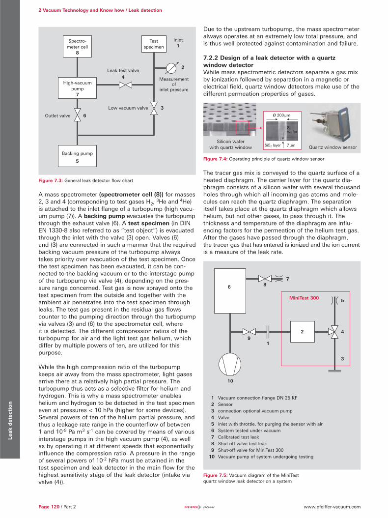
www.pfeiffer-vacuum.comPage 120 / Part 2
2 Vacuum Technology and Know how / Leak detectionLea
k d
etec
tion
Figure 7.3: General leak detector flow chart
A mass spectrometer (spectrometer cell (8)) for masses 2, 3 and 4 (corresponding to test gases H2, 3He and 4He) is attached to the inlet flange of a turbopump (high vacu-um pump (7)). A backing pump evacuates the turbopump through the exhaust valve (6). A test specimen (in DIN EN 1330-8 also referred to as “test object”) is evacuated through the inlet with the valve (3) open. Valves (6) and (3) are connected in such a manner that the required backing vacuum pressure of the turbopump always takes priority over evacuation of the test specimen. Once the test specimen has been evacuated, it can be con-nected to the backing vacuum or to the interstage pump of the turbopump via valve (4), depending on the pres-sure range concerned. Test gas is now sprayed onto the test specimen from the outside and together with the ambient air penetrates into the test specimen through leaks. The test gas present in the residual gas flows counter to the pumping direction through the turbopump via valves (3) and (6) to the spectrometer cell, where it is detected. The different compression ratios of the turbopump for air and the light test gas helium, which differ by multiple powers of ten, are utilized for this purpose.
While the high compression ratio of the turbopump keeps air away from the mass spectrometer, light gases arrive there at a relatively high partial pressure. The turbopump thus acts as a selective filter for helium and hydrogen. This is why a mass spectrometer enables helium and hydrogen to be detected in the test specimen even at pressures < 10 hPa (higher for some devices). Several powers of ten of the helium partial pressure, and thus a leakage rate range in the counterflow of between 1 and 10-9 Pa m3 s-1 can be covered by means of variousinterstage pumps in the high vacuum pump (4), as well as by operating it at different speeds that exponentiallyinfluence the compression ratio. A pressure in the range of several powers of 10-2 hPa must be attained in the test specimen and leak detector in the main flow for the highest sensitivity stage of the leak detector (intake via valve (4)).
Due to the upstream turbopump, the mass spectrometer always operates at an extremely low total pressure, and is thus well protected against contamination and failure.
7.2.2 Design of a leak detector with a quartz window detectorWhile mass spectrometric detectors separate a gas mix by ionization followed by separation in a magnetic or electrical field, quartz window detectors make use of the different permeation properties of gases.
Figure 7.4: Operating principle of quartz window sensor
The tracer gas mix is conveyed to the quartz surface of a heated diaphragm. The carrier layer for the quartz dia-phragm consists of a silicon wafer with several thousand holes through which all incoming gas atoms and mole-cules can reach the quartz diaphragm. The separation itself takes place at the quartz diaphragm which allows helium, but not other gases, to pass through it. The thickness and temperature of the diaphragm are influ-encing factors for the permeation of the helium test gas. After the gases have passed through the diaphragm, the tracer gas that has entered is ionized and the ion current is a measure of the leak rate.
Figure 7.5: Vacuum diagram of the MiniTest quartz window leak detector on a system
Spectro-meter cell
8
High-vacuum pump
7
6
3
Outlet valve
Low vacuum valve
Leak test valve
Backing pump
5
4
Test specimen
Inlet1
Measurementof
inlet pressure
2
1 Vacuum connection flange DN 25 KF 2 Sensor 3 connection optional vacuum pump 4 Valve 5 inlet with throttle, for purging the sensor with air 6 System tested under vacuum 7 Calibrated test leak 8 Shut-off valve test leak 9 Shut-off valve for MiniTest 300 10 Vacuum pump of system undergoing testing
6
3
4
5
2
87
9
MiniTest 300
Silicon waferwith quartz window Quartz window sensor
1
10
Ø 200 μm
7 μmSiO2 layer
Siwafer

www.pfeiffer-vacuum.com Part 2 / Page 121
2 Vacuum Technology and Know how / Leak detection
Lea
k d
etec
tion
The unit is connected to the system to be tested (6) with a vacuum connection flange (1). The connection (3) can optionally be connected to an additional vacuum pump. To prepare the leak test, this pump can evacuate the vacuum system of the unit while the shut-off valve (9) is still closed.
The shut-off valve (9) is opened for the test. The optional pump can generate a gas flow which reduces the response time of the sensor at higher system pressures.
The sensor (2) measures the partial pressure of helium in the vacuum. A test leak (7) on the system is used to determine the response time and calibrate the unit.
To protect the sensor and to purge the unit after a strong signal, automatic purging can be carried out. The valve (4) opens the inlet with the throttle (5) and the sensor is purged briefly with atmospheric air.
7.2.3 Test methodsThe test procedure used to detect leaks depends upon the type of test specimen and the required test results. The following criteria are formulated in the standard DIN EN 1779 [34]:
Will the test specimen be tested at overpressure or in a vacuum? In selecting the test method, if possible a method should be chosen that takes into account the pressure gradient encountered when the test specimen is actually used.
Is only a partial area or the whole area of the test specimen to be tested?
Should local leak detection, which is used to find leaks, be carried out or should integral leak detection, where the leakage rate of test specimens is typically determined for quality assurance purposes, be performed?
Leak detectors are equipped for two operating methods: The vacuum method, in which the test specimen is
evacuated and helium exerts its effect from the outside. The sniffer method, in which the workpiece is filled
with test gas overpressure � p > 100 hPa and the escaping test gas is sucked into the leak detector via a sniffer valve and detected.
7.2.4 Calibrating the leak detectorThe leak detector must be calibrated in order to determine leakage rates. This is done using a commercial test leak, which generates a known and reproducible test gas rate under defined conditions. Commercial test leaks are available in the form of a permeation leak or a capillary leak with or without a test gas reservoir. Leak detectors are usually equipped with permeation leaks with a helium reservoir. For calibration, an appropriate working cycle is often built in that automatically performs the calibration.
To obtain precise measurements, the unit should be calibrated before each use. To test large test specimens for which additional vacuum pumps are in use, it is advantageous to use an external test leak. The measure-
ment accuracy can depend on where the test leak is attached. Consequently, it is necessary to take flow conditions within the vacuum area into consideration. The use of external test leaks is also useful for deter-mining the maximum response time.
7.2.5 Local leak detectionLocal leak detection is used to identify leakage in a test specimen.
In the vacuum method, the test specimen (vessel) is connected to the leak detector, and helium is briefly sprayed onto a suspected area using a spray gun. If the pressure in the test specimen is in the molecular flow range, i. e. < 10-3 hPa, the test speed will be dependent on the volume of the test specimen and the effective pumping speed of the test setup for helium. The smaller the test specimen or the greater the pumping speed of the leak detector or auxiliary pump used, the quicker the result is obtained. At higher pressures, particularly in the laminar flow range greater than 1 hPa, the display speed will be much slower and will be governed by the pumping speed of the leak detector‘s backing pump.
In the sniffer method according to Figure 6 the test specimen (3) is filled with test gas overpressure. A sniffer probe (2) is connected to the test gas connection of the leak detector. The test gas that escapes through leaks in the test specimen can be detected by sniffing with the probe.
Figure 7.6: Local leak detection with sniffing and vacuum methods
Individual leaks can be identified using local leak detec-tion. However the sum of all leakage cannot be deter-mined. That is why this process offers only limited suit-ability for providing a GO / NO GO indication for quality assurance purposes.
Sniffer Leak Detection
Vacuum Leak Detection
Method Sniffing the test gas-filled test object
Spraying with helium
Mechanical strength
Against overpressure Against atmospheric pressure from the outside against vacuum (pressure difference 1000 hPa)
Detection limit < 1 · 10-8 Pa m3 s-1 < 5 · 10-13 Pa m3 s-1
Table 7.1: Local leak detection by sniffer and vacuum methods
Test gas
Test gas
3
2
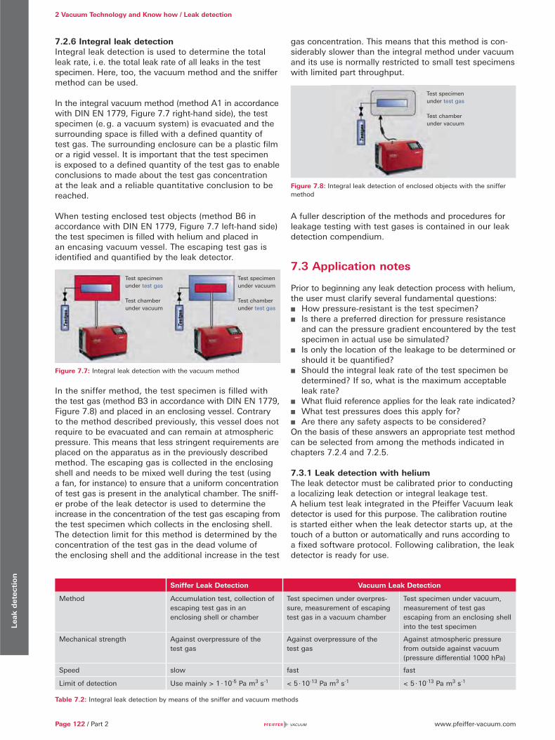
www.pfeiffer-vacuum.comPage 122 / Part 2
2 Vacuum Technology and Know how / Leak detectionLea
k d
etec
tion
7.2.6 Integral leak detectionIntegral leak detection is used to determine the total leak rate, i. e. the total leak rate of all leaks in the test specimen. Here, too, the vacuum method and the sniffer method can be used.
In the integral vacuum method (method A1 in accordance with DIN EN 1779, Figure 7.7 right-hand side), the test specimen (e. g. a vacuum system) is evacuated and the surrounding space is filled with a defined quantity of test gas. The surrounding enclosure can be a plastic film or a rigid vessel. It is important that the test specimen is exposed to a defined quantity of the test gas to enable conclusions to made about the test gas concentration at the leak and a reliable quantitative conclusion to be reached.
When testing enclosed test objects (method B6 in accordance with DIN EN 1779, Figure 7.7 left-hand side) the test specimen is filled with helium and placed in an encasing vacuum vessel. The escaping test gas is identified and quantified by the leak detector.
Figure 7.7: Integral leak detection with the vacuum method
In the sniffer method, the test specimen is filled with the test gas (method B3 in accordance with DIN EN 1779, Figure 7.8) and placed in an enclosing vessel. Contrary to the method described previously, this vessel does not require to be evacuated and can remain at atmospheric pressure. This means that less stringent requirements are placed on the apparatus as in the previously described method. The escaping gas is collected in the enclosing shell and needs to be mixed well during the test (using a fan, for instance) to ensure that a uniform concentration of test gas is present in the analytical chamber. The sniff-er probe of the leak detector is used to determine the increase in the concentration of the test gas escaping from the test specimen which collects in the enclosing shell. The detection limit for this method is determined by the concentration of the test gas in the dead volume of the enclosing shell and the additional increase in the test
Sniffer Leak Detection Vacuum Leak Detection
Method Accumulation test, collection of escaping test gas in an enclosing shell or chamber
Test specimen under overpres-sure, measurement of escaping test gas in a vacuum chamber
Test specimen under vacuum, measurement of test gas escaping from an enclosing shell into the test specimen
Mechanical strength Against overpressure of the test gas
Against overpressure of the test gas
Against atmospheric pressure from outside against vacuum (pressure differential 1000 hPa)
Speed slow fast fast
Limit of detection Use mainly > 1 · 10-5 Pa m3 s-1 < 5 · 10-13 Pa m3 s-1 < 5 · 10-13 Pa m3 s-1
gas concentration. This means that this method is con-siderably slower than the integral method under vacuum and its use is normally restricted to small test specimens with limited part throughput.
Figure 7.8: Integral leak detection of enclosed objects with the sniffer method
A fuller description of the methods and procedures for leakage testing with test gases is contained in our leak detection compendium.
7.3 Application notes
Prior to beginning any leak detection process with helium, the user must clarify several fundamental questions:
How pressure-resistant is the test specimen? Is there a preferred direction for pressure resistance
and can the pressure gradient encountered by the test specimen in actual use be simulated?
Is only the location of the leakage to be determined or should it be quantified?
Should the integral leak rate of the test specimen be determined? If so, what is the maximum acceptable leak rate?
What fluid reference applies for the leak rate indicated? What test pressures does this apply for? Are there any safety aspects to be considered?
On the basis of these answers an appropriate test method can be selected from among the methods indicated in chapters 7.2.4 and 7.2.5.
7.3.1 Leak detection with heliumThe leak detector must be calibrated prior to conducting a localizing leak detection or integral leakage test. A helium test leak integrated in the Pfeiffer Vacuum leak detector is used for this purpose. The calibration routine is started either when the leak detector starts up, at the touch of a button or automatically and runs according to a fixed software protocol. Following calibration, the leak detector is ready for use.
Table 7.2: Integral leak detection by means of the sniffer and vacuum methods
Test specimen under vacuum
Test chamber under test gas
Test specimen under test gas
Test chamber under vacuum
Test specimen under test gas
Test chamber under vacuum
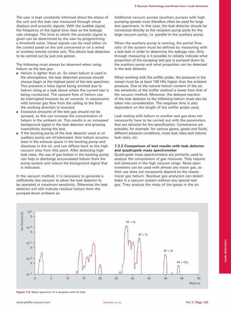
www.pfeiffer-vacuum.com Part 2 / Page 123
2 Vacuum Technology and Know how / Leak detection
Lea
k d
etec
tion
The user is kept constantly informed about the status of the unit and the leak rate measured through visual displays and acoustic signals. With the audible signal, the frequency of the signal tone rises as the leakage rate changes. The time at which the acoustic signal is given can be determined by the user by programming a threshold value. Visual signals can be read either on the control panel on the unit concerned or on a wired or wireless remote control unit. This allows leak detection to be carried out by just one person.
The following must always be observed when using helium as the test gas:
Helium is lighter than air. So when helium is used in the atmosphere, the leak detection process should always begin at the highest point of the test specimen. This prevents a false signal being emitted due to helium rising at a leak above where the current test is being conducted. The upward flow of helium can be interrupted however by air currents. In cleanrooms with laminar gas flow from the ceiling to the floor the working direction is reversed.
Excessive amounts of the test gas should not be sprayed, as this can increase the concentration of helium in the ambient air. This results in an increased background signal in the leak detector and growing insensitivity during the test.
If the backing pump of the leak detector used or an auxiliary pump are oil-lubricated, then helium accumu-lates in the exhaust space in the backing pump and dissolves in the oil, and can diffuse back to the high vacuum area from this point. After detecting high leak rates, the use of gas ballast in the backing pump can help to discharge accumulated helium from the pump system and reduce the background signal that is indicated.
In the vacuum method, it is necessary to generate a sufficiently low vacuum to allow the leak detector to be operated at maximum sensitivity. Otherwise the leak detector will still indicate residual helium from the pumped-down ambient air.
Additional vacuum pumps (auxiliary pumps) with high pumping speeds must therefore often be used for large test specimens. In this case, the leak detector should be connected directly to the recipient pump ports for the large vacuum pump, i.e. parallel to the auxiliary pump.
When the auxiliary pump is running, the partial flow ratio of the system must be defined by measuring with a test leak in order to determine the leakage rate. Only through measuring is it possible to reliably indicate what proportion of the escaping test gas is pumped down by the auxiliary pump and what proportion can be detected in the leak detector.
When working with the sniffer probe, the pressure in the vessel must be at least 100 hPa higher than the ambient pressure. Due to the natural helium content of the air, the sensitivity of the sniffer method is lower than that of the vacuum method. Moreover, the delayed reaction of the leak detector to the inflowing helium must also be taken into consideration. The response time is also dependent on the length of the sniffer probe used.
Leak testing with helium or another test gas does not necessarily have to be carried out with the parameters that are decisive for the specification. Conversions are possible, for example, for various gases, gases and fluids, different pressure conditions, mass leak rates and volume leak rates, etc.
7.3.2 Comparison of test results with leak detector and quadrupole mass spectrometerQuadrupole mass spectrometers are primarily used to analyze the composition of gas mixtures. They require test pressures in the high vacuum range. Mass spec-trometers can be used with almost any tracer gas, as their use does not necessarily depend on the classic tracer gas helium. Residual gas analyzers can detect leaks in a vacuum system without any special test gas. They analyze the mass of the gases in the air.
Figure 7.9: Mass spectrum of a recipient with air leak
10-9
5
10-10
5
10-11
5
10-12
5
10-13
Ion
Cu
rren
t [A
]
0 5 10 15 20 25 30 35 40 45 50
Mass [u]
32 = O2
40 = Ar
44 = CO2
28 = N2
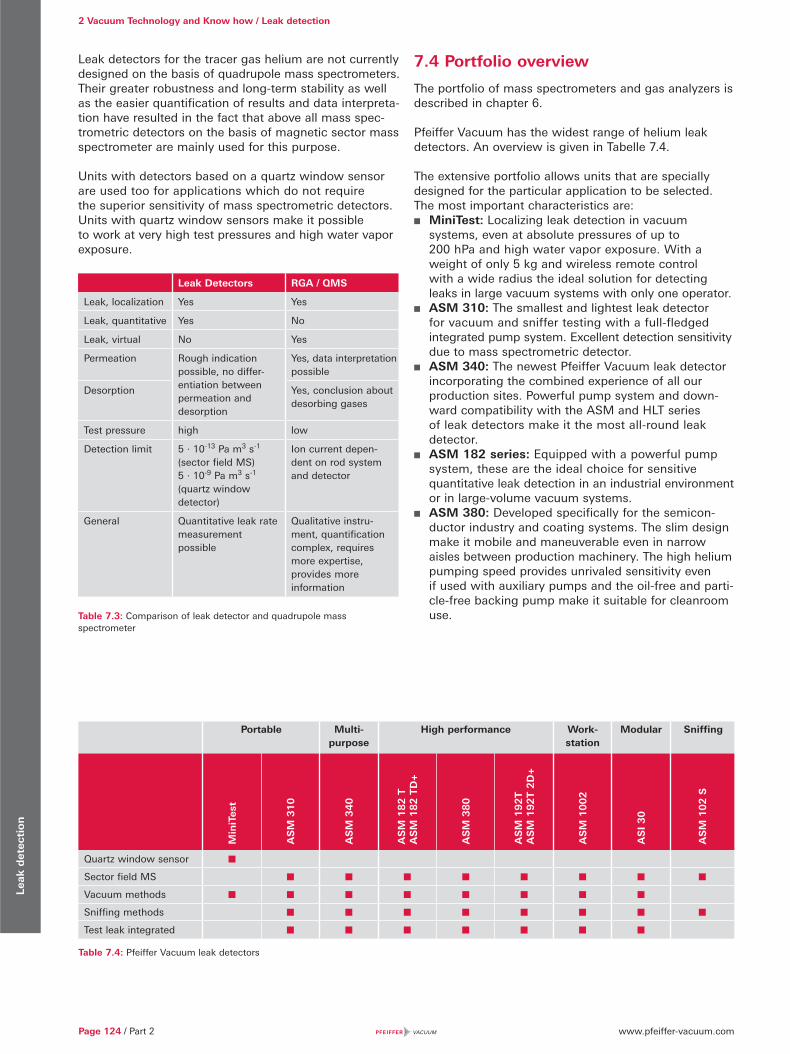
www.pfeiffer-vacuum.comPage 124 / Part 2
2 Vacuum Technology and Know how / Leak detectionLea
k d
etec
tion
Leak detectors for the tracer gas helium are not currently designed on the basis of quadrupole mass spectrometers. Their greater robustness and long-term stability as well as the easier quantification of results and data interpreta-tion have resulted in the fact that above all mass spec-trometric detectors on the basis of magnetic sector mass spectrometer are mainly used for this purpose.
Units with detectors based on a quartz window sensor are used too for applications which do not require the superior sensitivity of mass spectrometric detectors. Units with quartz window sensors make it possible to work at very high test pressures and high water vapor exposure.
Leak Detectors RGA / QMS
Leak, localization Yes Yes
Leak, quantitative Yes No
Leak, virtual No Yes
Permeation Rough indication possible, no differ-entiation between permeation and desorption
Yes, data interpretation possible
Desorption Yes, conclusion about desorbing gases
Test pressure high low
Detection limit 5 · 10-13 Pa m3 s-1 (sector field MS)5 · 10-9 Pa m3 s-1 (quartz window detector)
Ion current depen-dent on rod system and detector
General Quantitative leak rate measurement possible
Qualitative instru-ment, quantification complex, requires more expertise, provides more information
Table 7.3: Comparison of leak detector and quadrupole mass spectrometer
7.4 Portfolio overview
The portfolio of mass spectrometers and gas analyzers is described in chapter 6.
Pfeiffer Vacuum has the widest range of helium leak detectors. An overview is given in Tabelle 7.4.
The extensive portfolio allows units that are specially designed for the particular application to be selected. The most important characteristics are:
MiniTest: Localizing leak detection in vacuum systems, even at absolute pressures of up to 200 hPa and high water vapor exposure. With a weight of only 5 kg and wireless remote control with a wide radius the ideal solution for detecting leaks in large vacuum systems with only one operator.
ASM 310: The smallest and lightest leak detector for vacuum and sniffer testing with a full-fledged integrated pump system. Excellent detection sensitivity due to mass spectrometric detector.
ASM 340: The newest Pfeiffer Vacuum leak detector incorporating the combined experience of all our production sites. Powerful pump system and down-ward compatibility with the ASM and HLT series of leak detectors make it the most all-round leak detector.
ASM 182 series: Equipped with a powerful pump system, these are the ideal choice for sensitive quantitative leak detection in an industrial environment or in large-volume vacuum systems.
ASM 380: Developed specifically for the semicon-ductor industry and coating systems. The slim design make it mobile and maneuverable even in narrow aisles between production machinery. The high helium pumping speed provides unrivaled sensitivity even if used with auxiliary pumps and the oil-free and parti-cle-free backing pump make it suitable for cleanroom use.
Portable Multi- purpose
High performance Work-station
Modular Sniffing
Min
iTes
t
AS
M 3
10
AS
M 3
40
AS
M 1
82
TA
SM
18
2 T
D+
AS
M 3
80
AS
M 1
92
TA
SM
19
2T 2
D+
AS
M 1
00
2
AS
I 3
0
AS
M 1
02
S
Quartz window sensor
Sector field MS
Vacuum methods
Sniffing methods
Test leak integrated
Table 7.4: Pfeiffer Vacuum leak detectors
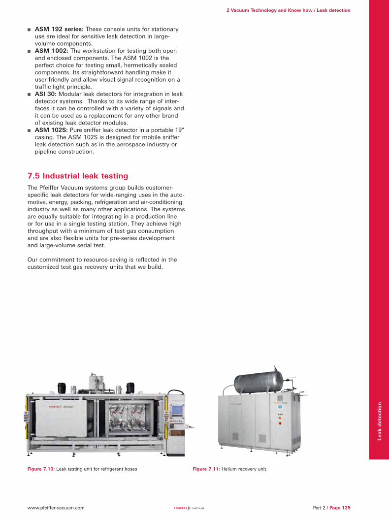
www.pfeiffer-vacuum.com Part 2 / Page 125
2 Vacuum Technology and Know how / Leak detection
Lea
k d
etec
tion
ASM 192 series: These console units for stationary use are ideal for sensitive leak detection in large- volume components.
ASM 1002: The workstation for testing both open and enclosed components. The ASM 1002 is the perfect choice for testing small, hermetically sealed components. Its straightforward handling make it user-friendly and allow visual signal recognition on a traffic light principle.
ASI 30: Modular leak detectors for integration in leak detector systems. Thanks to its wide range of inter-faces it can be controlled with a variety of signals and it can be used as a replacement for any other brand of existing leak detector modules.
ASM 102S: Pure sniffer leak detector in a portable 19" casing. The ASM 102S is designed for mobile sniffer leak detection such as in the aerospace industry or pipeline construction.
7.5 Industrial leak testingThe Pfeiffer Vacuum systems group builds customer- specific leak detectors for wide-ranging uses in the auto-motive, energy, packing, refrigeration and air-conditioning industry as well as many other applications. The systems are equally suitable for integrating in a production line or for use in a single testing station. They achieve high throughput with a minimum of test gas consumption and are also flexible units for pre-series development and large-volume serial test.
Our commitment to resource-saving is reflected in the customized test gas recovery units that we build.
Figure 7.10: Leak testing unit for refrigerant hoses Figure 7.11: Helium recovery unit

www.pfeiffer-vacuum.comSeite 126 / Band 2
Con
tam
inat
ion
m
anag
emen
t so
luti
ons
8 Contamination management solutions
8.1 Introduction
In semiconductor manufacturing, i.e. the production of integrated electronic circuits, many crucial process steps are based on vacuum technology. There are several reasons for the use of vacuum technology in Silicon processing:
Vacuum allows controlled conditions as it excludes the ambient atmosphere from the silicon wafer, namely reactive gases and dust.
Vacuum allows anisotropic etching of silicon and silicon oxide, the basic process steps for patterning the surface of the silicon wafer.
Several vacuum based processes allow the deposition of thin layers of all types of insulation and conducting films with controllable properties on silicon wafers.
The development of integrated circuits made from solid silicon is characterized by a steady increase of perfor-mance due to an ever increasing number of integrated components per device and shrinkage of the pattern size. In the course of his development the performance of the circuits has doubled approximately every two years since the 1960s which has been predicted by Gordon E. Moore and is known as Moore’s law [35]. This has been achieved by a reduction of the smallest structures
of integrated circuits like microprocessors and random access memory from about 10 μm in 1970 to sub 0.1 μm after the turn of the millennium. During this period the size of the silicon wafers increased from 1" diameter to 300 mm (~12") to improve throughput and reduce cost.
With the introduction of the 300 mm technology the so called critical dimensions shrank from 150 nm and have reached 22 nm at the time this text is written (2012). With 300 mm wafer size the production technology also changed from open cassettes (Figure 8.2 left) to closed mini environment, i.e. the wafers are transferred from one process equipment to another inside the production site in closed boxes (FOUP = Front Opening Unified Pod, Figure 8.2 right).
Figure 8.2: Wafer handling with cassettes (left) and FOUPs (right)
Figure 8.1: Moore’s Law (documented by the number of transistors in Intel and AMD microprocessors)
1971 1980 1990 2000 20111971 1980 1990 2000 2011
Tran
sist
or
cou
nt 2,600,000,000
1,000,000,000
100,000,000
10,000,000
1,000,000
100,000
10,000
2,300 40048008
80806800
8086
RCA 1802MOS 6502
Z806809
80888006
68000
80286
80386
80486
PentiumAMD K5
Pentium IIPentium III
Pentium 4
AMD K6
AMD K8
Barion Atom
CelCore 2 Duo
AMD K6-III / AMD K7
80186
Core i7 (Quad)Six-Core-Option 2400
8-Core Xeon Nehalem-EX
10-Core Xeon Westmere-EX16-Core SPARC T3
Six-Core Core i7
Six-Core Xeon 7400
Dual-Core Itanium 2AMD K10
AMD K10
POWER6Itanium 2 with 9 MB cache
Itanium 2
8-Core POWER7
Quad-Core Itanium TukwilaQuad-Core 2196
curve shows transistor count doubling every two years
Date of introduction

www.pfeiffer-vacuum.com Band 2 / Seite 127
2 Vacuum Technology and Know how / Contamination management solutions
Con
tam
inat
ion
m
anag
emen
t so
luti
ons
The International Technology Roadmap for Semiconduc-tors (ITRS) has established a list of AMCs which can provoke wafer defects [36]. This list comprises inorganic and organic acids, bases, sulphur compounds, and volatile organic compounds, see figure 8.4 for details.
There are two main sources of AMC in the FOUPs inner atmosphere. The main source are the wafers stored in the FOUP after each process step. Byproducts from the last process are released from their surface and can be absorbed by the polymer material of the FOUP or reabsorbed on other wafer surfaces. The second source is outgassing from the FOUP, either from the bulk of the polymer or from previously absorbed byproducts of other wafers and/or other processes. As polymers have a high capacity to absorb gases, the FOUP has a “memory” of the wafers it has carried. Compared to these AMC sources the contribution of the well controlled clean room air can be neglected.
Figure 8.5: AMC Sources in FOUPs
8.2 Contamination
Dust is the natural enemy of integrated circuit manufac-turing of small sized devices. In the course of the devel-opment of integrated circuits efficient methods have been developed to eliminate dust from the production environment. A dust particle of a size comparable with the elements of the circuit structure (critical dimension, CD) or larger can be problematic if it is accidentally incorporated into the device. A structure of 22 nm of silicon comprises only 41 Si atoms. On this scale not only particles present a challenge but contamination by molecules becomes an increasing challenge. Those contaminations are known as airborne molecular contamination (AMC). The change from open cassettes to closed FOUPs reduced largely particle contamination but at the same time increased the impact of AMC.
Figure 8.3: Diamondlike crystal structure of Silicon
Molecules on the surface of the wafer which originate from the ambiant air, released from the surrounding surfaces, or from a preceding process step can react with atmospheric gases forming minuscule clusters of reaction products which tend to grow during queue time when wafers are waiting for the next process step. The nucleus of molecular contamination usually is from the many compounds used in semiconductor fabrication.
Figure 8.4: Classification of airborne molecular contamination AMC
Cleanroom contamination
Wafer outgassing
FOUP outgassing
ACIDS BASES
CONDENSABLES DOPANTS
NOxNH3HCI
H2SO4
H2S
SOx
HFH2O2
IPA
O3
Acetone
NO CLASSES
Organosulfates
DOP
Silicones ToluolTrisilanol Siloxanes BHT
AminesMethylamineTriethylamineNMP
Amides
B2O3
BF3
Organophosphates TEP
TCPP
O = PO C3H6 CIO C3H6 CIO C3H6 CI
CO-OCH2-CH-C4H9
C2H5
C2H5
CO-OCH2-CH-C4H9
Categories of AMC and typical compounds
OH

www.pfeiffer-vacuum.comSeite 128 / Band 2
2 Vacuum Technology and Know how / Contamination management solutionsC
onta
min
atio
n
man
agem
ent
solu
tion
s
8.3 The nature of AMC
At atmospheric pressure and ambient temperature a solid surface, which incorporates about 1015 atoms/cm2 receives a flow of incident gas molecules and atoms of the order of 1023 [37] per second and square centimeter. This means within nanoseconds the surface will be covered by some layers of gas molecules. The probability of a molecule to stick on the surface depends largely on its nature and the nature and topography of the surface. But even minor traces of reaction by-products in the ppbv range (parts per billion of volume, i. e. 10-9) which hit the surface at a rate of 1014 s-1 cm-2 will cover a surface within seconds if the sticking coefficient is high.
Airborne molecules can be either polar or non polar. In non polar molecules the electrical charges are symmetri-cally distributed, the centers of positive and negative charges coincide. Examples are nitrogen N2 or the linear CO2 molecule. These molecules are kept on a solid surface by weak van der Waals forces, with binding energies typically ranging between thermal energy RT ≈ 2.5 kJ/mol and about 20 · RT. In polar molecules the electrical charges are asymmetrically distributed result-ing in a permanent dipolar momentum. Examples for polar molecules are water H2O and inorganic acids used in semiconductor etching processes like HF and HCl. Binding energies of polar molecules are higher, e. g. for H2O on a Si(100) surface about 138 kJ/mol. These molecules are likely to interact chemically with the surface, forming nuclei for further reactions.
8.4 From surface molecular contamination (SMC) to defects
The different phenomena at the interaction plane between a solid surface and a gas are shown in figure 8.7. Gas molecules impinge on the solid, diffuse along the surface, and desorb or get adsorbed to it. A solid surface is the boundary between the bulk material and the outer world. This surface has higher energy than the bulk material because of the pending dangling bonds of the last layer of atoms or molecules. Each of the pending dangling bonds is a potential adsorption site. The free energy of the surface depends on the nature of the material bonds, i.e. metallic, ionic or covalent. The number of adsorption sites increases from well ordered crystal surfaces to polycrystalline and to amorphous polymer materials. Any irregularity increases the number of adsorption sites.
Water vapor plays a special rule in surface processes. At 25 °C and 50 % relative humidity, air contains 16 hPa (1.58 %) of water vapor. Any surface receives a flux of water molecules of about 5 · 1021 cm-2 s-1. In about 200 ns a Mono layer of water could cover a Si (100) surface. Due to the polar nature of the water molecule the first layer will bond tightly to the surfaces and addi-tional layers of water-to-water bonds will form resulting in a stack of water layers. An acid molecule arriving on a surface exposed to atmospheric conditions will meet water molecules to assist in further reactions.Any material that is capable of absorbing water into the bulk such as plastics or elastomers, will become saturat-ed if it is exposed long enough.
Figure 8.6: Airborne polar and non polar molecules
Figure 8.8: Surface sites
Figure 8.7: Gas-solid interaction at a surface
IncomingDiffusion
Desorption
Adsorption
terrace
ad-atom
i = 1
i = 3i = 3
i = 0
step edgeisland
vacancy i = 4 kink site i = 2
CO2
N2
HF
HCI
H2O
NH3
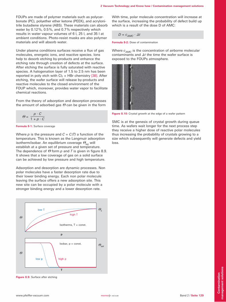
www.pfeiffer-vacuum.com Band 2 / Seite 129
2 Vacuum Technology and Know how / Contamination management solutions
Con
tam
inat
ion
m
anag
emen
t so
luti
ons
FOUPs are made of polymer materials such as polycar-bonate (PC), polyether ether ketone (PEEK), and acryloni-trile butadiene styrene (ABS). These materials can absorb water by 0.12 %, 0.5 %, and 0.7 % respectively which results in water vapour volumes of 6 l, 25 l, and 35 l at ambient conditions. Photo-resist masks are also polymer materials and will absorb water.
Under plasma conditions surfaces receive a flux of gas molecules, energetic ions, and reactive species. Ions help to desorb etching by-products and enhance the etching rate through creation of defects at the surface. After etching the surface is fully saturated with reactive species. A halogenation layer of 1.5 to 2.5 nm has been reported in poly etch with Cl2 + HBr chemistry [38]. After etching, the wafer surface will release by-products and reactive molecules to the closed environment of the FOUP which, moreover, provides water vapor to facilitate chemical reactions.
From the theory of adsorption and desorption processes the amount of adsorbed gas can be given in the form
Formula 8-1: Surface coverage
Where p is the pressure and C = C (T) a function of the temperature. This is known as the Langmuir adsorption isotherm/isobar. An equilibrium coverage eq will establish at a given set of pressure and temperature. The dependence of form p and T is given in figure 8.9. It shows that a low coverage of gas on a solid surface can be achieved by low pressure and high temperature.
Adsorption and desorption are dynamic processes. Non polar molecules have a faster desorption rate due to their lower binding energy. Each non polar molecule leaving the surface offers a new adsorption site. This new site can be occupied by a polar molecule with a stronger binding energy and a lower desorption rate.
With time, polar molecule concentration will increase at the surface, increasing the probability of defect build up which is a result of the dose D of AMC:
Formula 8-2: Dose of contamination
Where cAMC is the concentration of airborne molecular contaminants and � t the time the wafer surface is exposed to the FOUPs atmosphere.
Figure 8.10: Crystal growth at the edge of a wafer pattern
SMC is at the genesis of crystal growth during queue time. As wafers wait longer for the next process step they receive a higher dose of reactive polar molecules thus increasing the probability of crystals growing to a size which subsequently will generate defects and yield loss.
D = cAMC · � t
s
sat
Isotherms, T = const.
Isobar, p = const.
p
T
low T
high T
low p high p
= p · C
1 + p · C
Figure 8.9: Surface after etching
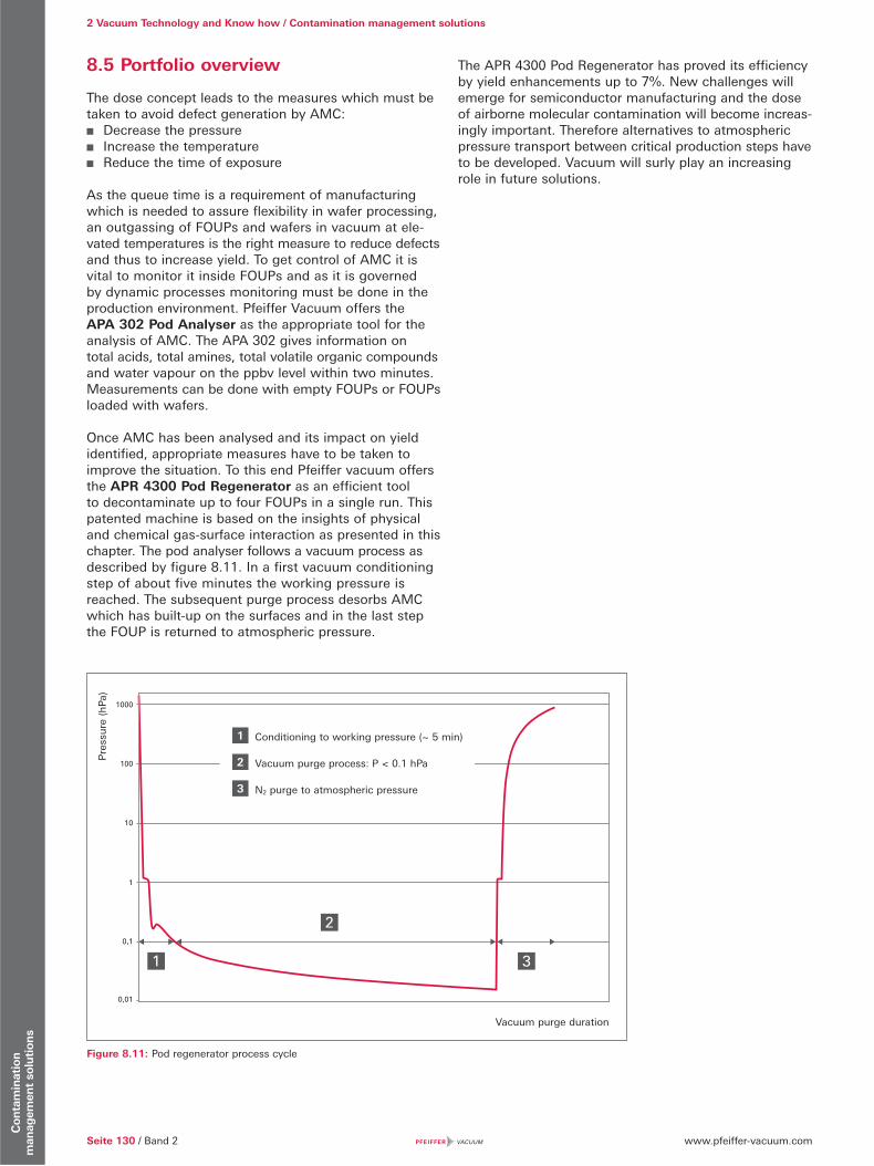
www.pfeiffer-vacuum.comSeite 130 / Band 2
2 Vacuum Technology and Know how / Contamination management solutionsC
onta
min
atio
n
man
agem
ent
solu
tion
s
8.5 Portfolio overview
The dose concept leads to the measures which must be taken to avoid defect generation by AMC:
Decrease the pressure Increase the temperature Reduce the time of exposure
As the queue time is a requirement of manufacturing which is needed to assure flexibility in wafer processing, an outgassing of FOUPs and wafers in vacuum at ele-vated temperatures is the right measure to reduce defects and thus to increase yield. To get control of AMC it is vital to monitor it inside FOUPs and as it is governed by dynamic processes monitoring must be done in the production environment. Pfeiffer Vacuum offers the APA 302 Pod Analyser as the appropriate tool for the analysis of AMC. The APA 302 gives information on total acids, total amines, total volatile organic compounds and water vapour on the ppbv level within two minutes. Measurements can be done with empty FOUPs or FOUPs loaded with wafers.
Once AMC has been analysed and its impact on yield identified, appropriate measures have to be taken to improve the situation. To this end Pfeiffer vacuum offers the APR 4300 Pod Regenerator as an efficient tool to decontaminate up to four FOUPs in a single run. This patented machine is based on the insights of physical and chemical gas-surface interaction as presented in this chapter. The pod analyser follows a vacuum process as described by figure 8.11. In a first vacuum conditioning step of about five minutes the working pressure is reached. The subsequent purge process desorbs AMC which has built-up on the surfaces and in the last step the FOUP is returned to atmospheric pressure.
Figure 8.11: Pod regenerator process cycle
The APR 4300 Pod Regenerator has proved its efficiency by yield enhancements up to 7%. New challenges will emerge for semiconductor manufacturing and the dose of airborne molecular contamination will become increas-ingly important. Therefore alternatives to atmospheric pressure transport between critical production steps have to be developed. Vacuum will surly play an increasing role in future solutions.
0,01
1 3
20,1
1
10
100
1000
Pre
ssu
re (
mb
ar)
Vacuum purge duration
Pre
ssu
re (
hPa)
Vacuum purge duration
1 Conditioning to working pressure (~ 5 min)
2 Vacuum purge process: P < 0.1 hPa
3 N2 purge to atmospheric pressure
www.pfeiffer-vacuum.com Band 2 / Seite 131
2 Vacuum Technology and Know how / Contamination management solutions
Con
tam
inat
ion
m
anag
emen
t so
luti
ons
Page 132 / Part 2 www.pfeiffer-vacuum.com
Index
1 Introduction to vacuum technology
Figure 1.1: Overview of vacuum . . . . . . . . . . . . . . . . . . . . . . . . . . . . . . . . . . . . . . . . . . . . . . . . . . . . . . . . . . . 8
Figure 1.2: Definition of total pressure . . . . . . . . . . . . . . . . . . . . . . . . . . . . . . . . . . . . . . . . . . . . . . . . . . . . . . 9
Figure 1.3: Definition of partial pressure . . . . . . . . . . . . . . . . . . . . . . . . . . . . . . . . . . . . . . . . . . . . . . . . . . . . 10
Figure 1.4: Mean free path between two collisions . . . . . . . . . . . . . . . . . . . . . . . . . . . . . . . . . . . . . . . . . . . . 12
Figure 1.5: Molecular number density (red, right-hand y axis) and
mean free path (blue, left-hand y axis) for nitrogen at a temperature of 273.15 K. . . . . . . . . . . 13
Figure 1.6: Profiles of the various types of flow regimes . . . . . . . . . . . . . . . . . . . . . . . . . . . . . . . . . . . . . . . 14
Figure 1.7: Flow ranges in vacuum as a function of p · d . . . . . . . . . . . . . . . . . . . . . . . . . . . . . . . . . . . . . . . 15
Figure 1.8: Conductance of a smooth round pipe as a function
of the mean pressure in the pipe . . . . . . . . . . . . . . . . . . . . . . . . . . . . . . . . . . . . . . . . . . . . . . . . . 16
Figure 1.9: Vapor pressure curves of various substances . . . . . . . . . . . . . . . . . . . . . . . . . . . . . . . . . . . . . . . 17
Figure 1.10: Typical residual gas spectrum of a vessel evacuated by a turbomolecular pump . . . . . . . . . . . 20
Figure 2.1: No-load compression ratio for air with Roots pumps . . . . . . . . . . . . . . . . . . . . . . . . . . . . . . . . . 24
Figure 2.2: Volume flow rate (pumping speed) of a pumping station with Hepta 100 and Okta 500 . . . . . 24
Figure 2.3: Drying system (schematic) . . . . . . . . . . . . . . . . . . . . . . . . . . . . . . . . . . . . . . . . . . . . . . . . . . . . . . 25
Figure 2.4: Roots pumping station for vapor condensation . . . . . . . . . . . . . . . . . . . . . . . . . . . . . . . . . . . . . 26
Figure 2.5: Roots pumping station for vapor condensation . . . . . . . . . . . . . . . . . . . . . . . . . . . . . . . . . . . . . 27
Figure 2.6: Roots pumping station for transformer drying . . . . . . . . . . . . . . . . . . . . . . . . . . . . . . . . . . . . . . 27
Figure 2.7: Gas throughput of different turbopumps at high process pressures . . . . . . . . . . . . . . . . . . . . . 29
Figure 2.8: Vacuum system with pressure and throughput regulation . . . . . . . . . . . . . . . . . . . . . . . . . . . . . 30
Figure 3.1: Temperature dependence of the elasticity modulus of austenitic stainless steel . . . . . . . . . . . . 34
Figure 3.2: Temperature dependence of the 0.2 % yield point of austenitic stainless steel . . . . . . . . . . . . . 34
Figure 3.3: De Long diagram . . . . . . . . . . . . . . . . . . . . . . . . . . . . . . . . . . . . . . . . . . . . . . . . . . . . . . . . . . . . . 35
Figure 3.4: Cross section image of a laser weld . . . . . . . . . . . . . . . . . . . . . . . . . . . . . . . . . . . . . . . . . . . . . . 39
Figure 3.5: Cross section image of WIG orbital weld . . . . . . . . . . . . . . . . . . . . . . . . . . . . . . . . . . . . . . . . . . 39
Figure 3.6: O-ring seals in rectangular groove, trapezoidal-groove and in an angular position . . . . . . . . . . 41
Figure 3.7: ISO-KF connection with centering ring and clamping ring . . . . . . . . . . . . . . . . . . . . . . . . . . . . . 41
Figure 3.8: ISO-KF flange mounted on base plate with centering ring and claw clamps . . . . . . . . . . . . . . . 41
Figure 3.9: ISO-K connection with centering ring and double claw clamps . . . . . . . . . . . . . . . . . . . . . . . . . 42
Figure 3.10: ISO-K flange mounted on base plate with centering ring and claw clamps . . . . . . . . . . . . . . . . 42
Figure 3.11: ISO-K flange mounted on base plate with O-ring nut
and claw clamps for base plate with sealing groove . . . . . . . . . . . . . . . . . . . . . . . . . . . . . . . . . 42
Figure 3.12: ISO-K flange mounted on base plate with centering ring, bolt ring and screws . . . . . . . . . . . . 42
Figure 3.13: ISO-F connection with centering ring and screws . . . . . . . . . . . . . . . . . . . . . . . . . . . . . . . . . . . 43
Figure 3.14: ISO-K flange with bolt ring mounted on ISO-F flange with centering ring and screws . . . . . . . 43
Figure 3.15: CF connection with copper flat gasket and screws . . . . . . . . . . . . . . . . . . . . . . . . . . . . . . . . . . 43
Figure 3.16: COF connection with copper wire seal and screws . . . . . . . . . . . . . . . . . . . . . . . . . . . . . . . . . . 44
Figure 3.17: EUV source chamber with cooling profiles and water-cooled flanges . . . . . . . . . . . . . . . . . . . . 47
Figure 3.18: Space simulation chamber with pillow plate cooling . . . . . . . . . . . . . . . . . . . . . . . . . . . . . . . . . 47
Figure 3.19: CF viewport with glass-metal fusing . . . . . . . . . . . . . . . . . . . . . . . . . . . . . . . . . . . . . . . . . . . . . . 49
Figure 3.20: Electrical feedthrough with ceramically insulated wire conductor made of copper . . . . . . . . . . 50
Figure 3.21: Bellows-sealed angle valve . . . . . . . . . . . . . . . . . . . . . . . . . . . . . . . . . . . . . . . . . . . . . . . . . . . . . 51
Figure 3.22: Inline valve with electropneumatic actuation . . . . . . . . . . . . . . . . . . . . . . . . . . . . . . . . . . . . . . . 51
Index of figures
2 Basic calculations
3 Mechanicalcomponents in vacuum
www.pfeiffer-vacuum.com Part 2 / Page 133
Vacuum Technology and Know how / Index
Figure 3.23: UHV gate valve . . . . . . . . . . . . . . . . . . . . . . . . . . . . . . . . . . . . . . . . . . . . . . . . . . . . . . . . . . . . . . 52
Figure 3.24: UHV all-metal gas-dosing valve . . . . . . . . . . . . . . . . . . . . . . . . . . . . . . . . . . . . . . . . . . . . . . . . . . 52
Figure 3.25: Bellows-sealed UHV rotary feedthrough (cattail principle) . . . . . . . . . . . . . . . . . . . . . . . . . . . . . 53
Figure 3.26: Magnetically coupled UHV rotary feedthrough . . . . . . . . . . . . . . . . . . . . . . . . . . . . . . . . . . . . . . 54
Figure 3.27: Elastomer-sealed rotary feedthrough . . . . . . . . . . . . . . . . . . . . . . . . . . . . . . . . . . . . . . . . . . . . . . 54
Figure 3.28: Z-axis precision manipulator . . . . . . . . . . . . . . . . . . . . . . . . . . . . . . . . . . . . . . . . . . . . . . . . . . . . 55
Figure 3.29: XY-axis precision manipulator . . . . . . . . . . . . . . . . . . . . . . . . . . . . . . . . . . . . . . . . . . . . . . . . . . . 56
Figure 4.1: Overview of vacuum pumps . . . . . . . . . . . . . . . . . . . . . . . . . . . . . . . . . . . . . . . . . . . . . . . . . . . . 58
Figure 4.2: Operating principle of a rotary vane pump . . . . . . . . . . . . . . . . . . . . . . . . . . . . . . . . . . . . . . . . . 60
Figure 4.3: Pfeiffer Vacuum rotary vane pumps . . . . . . . . . . . . . . . . . . . . . . . . . . . . . . . . . . . . . . . . . . . . . . 62
Figure 4.4: Accessories for rotary vane pumps . . . . . . . . . . . . . . . . . . . . . . . . . . . . . . . . . . . . . . . . . . . . . . . 67
Figure 4.5: Operating principle of a diaphragm vacuum pump . . . . . . . . . . . . . . . . . . . . . . . . . . . . . . . . . . . 68
Figure 4.6: Operating principle of a screw pump . . . . . . . . . . . . . . . . . . . . . . . . . . . . . . . . . . . . . . . . . . . . . 69
Figure 4.7: HeptaDry rotors . . . . . . . . . . . . . . . . . . . . . . . . . . . . . . . . . . . . . . . . . . . . . . . . . . . . . . . . . . . . . . 69
Figure 4.8: HeptaDry with connections and accessories. . . . . . . . . . . . . . . . . . . . . . . . . . . . . . . . . . . . . . . . 70
Figure 4.9: Operating principle of an air cooled multi-stage Roots pump . . . . . . . . . . . . . . . . . . . . . . . . . . 71
Figure 4.10: Condensation of ammonium hexafluorosilicate (NH4)2SiF6 in a Roots pump
operated at too low a temperature . . . . . . . . . . . . . . . . . . . . . . . . . . . . . . . . . . . . . . . . . . . . . . . 74
Figure 4.11: Operating principle of a multi-stage Roots pump, process pump . . . . . . . . . . . . . . . . . . . . . . . 74
Figure 4.12: ACP 120 . . . . . . . . . . . . . . . . . . . . . . . . . . . . . . . . . . . . . . . . . . . . . . . . . . . . . . . . . . . . . . . . . . . . 75
Figure 4.13: A 100 L rear side with connections . . . . . . . . . . . . . . . . . . . . . . . . . . . . . . . . . . . . . . . . . . . . . . . 76
Figure 4.14: A 203 H cross-section . . . . . . . . . . . . . . . . . . . . . . . . . . . . . . . . . . . . . . . . . . . . . . . . . . . . . . . . . 76
Figure 4.15: A 1503 H process pumping station . . . . . . . . . . . . . . . . . . . . . . . . . . . . . . . . . . . . . . . . . . . . . . . 77
Figure 4.16: Operating principle of a Roots pump . . . . . . . . . . . . . . . . . . . . . . . . . . . . . . . . . . . . . . . . . . . . . . 78
Figure 4.17: Operating principle of a gas cooled Roots pump . . . . . . . . . . . . . . . . . . . . . . . . . . . . . . . . . . . . 79
Figure 4.18: No-load compression ratio for air for Roots pumps . . . . . . . . . . . . . . . . . . . . . . . . . . . . . . . . . . 79
Figure 4.19: Pumping speed of pumping stations with Okta 2000 and various backing pumps . . . . . . . . . . 80
Figure 4.20: Operating principle of a side channel vacuum pump . . . . . . . . . . . . . . . . . . . . . . . . . . . . . . . . . 83
Figure 4.21: Degrees of freedom of a turbo-rotor . . . . . . . . . . . . . . . . . . . . . . . . . . . . . . . . . . . . . . . . . . . . . . 84
Figure 4.22: Operating principle of the turbomolecular pump . . . . . . . . . . . . . . . . . . . . . . . . . . . . . . . . . . . . 84
Figure 4.23: Specific turbopump pumping speeds . . . . . . . . . . . . . . . . . . . . . . . . . . . . . . . . . . . . . . . . . . . . . 85
Figure 4.24: Pumping speed as a function of relative molecular mass . . . . . . . . . . . . . . . . . . . . . . . . . . . . . . 85
Figure 4.25: Pumping speed as a function of inlet pressure . . . . . . . . . . . . . . . . . . . . . . . . . . . . . . . . . . . . . . 85
Figure 4.26: Operating principle of a Holweck stage . . . . . . . . . . . . . . . . . . . . . . . . . . . . . . . . . . . . . . . . . . . 86
Figure 4.27: Compression ratios of pure turbopumps and turbo drag pumps . . . . . . . . . . . . . . . . . . . . . . . . 86
Figure 4.28: Typical UHV residual gas spectrum (turbopump) . . . . . . . . . . . . . . . . . . . . . . . . . . . . . . . . . . . . 87
Figure 4.29: Standard HiPace turbopumps . . . . . . . . . . . . . . . . . . . . . . . . . . . . . . . . . . . . . . . . . . . . . . . . . . . 89
Figure 4.30: ATH M magnetic-levitation turbopump . . . . . . . . . . . . . . . . . . . . . . . . . . . . . . . . . . . . . . . . . . . . 90
Figure 4.31: Example of turbopump accessories (for HiPace 300) . . . . . . . . . . . . . . . . . . . . . . . . . . . . . . . . . 91
Figure 5.1: Design of a diaphragm vacuum gauge . . . . . . . . . . . . . . . . . . . . . . . . . . . . . . . . . . . . . . . . . . . . 92
Figure 5.2: Design of a capacitative diaphragm vacuum gauge . . . . . . . . . . . . . . . . . . . . . . . . . . . . . . . . . . 93
Figure 5.3: Operating principle of the Pirani vacuum gauge . . . . . . . . . . . . . . . . . . . . . . . . . . . . . . . . . . . . . 93
Figure 5.4: Pirani vacuum gauge curves . . . . . . . . . . . . . . . . . . . . . . . . . . . . . . . . . . . . . . . . . . . . . . . . . . . . 94
Figure 5.5: Design of an inverted magnetron . . . . . . . . . . . . . . . . . . . . . . . . . . . . . . . . . . . . . . . . . . . . . . . . 94
Figure 5.6: Operating principle of an inverted magnetron . . . . . . . . . . . . . . . . . . . . . . . . . . . . . . . . . . . . . . . 94
Figure 5.7: Design of a Bayard-Alpert vacuum gauge . . . . . . . . . . . . . . . . . . . . . . . . . . . . . . . . . . . . . . . . . . 95
Figure 5.8: Pressure measurement ranges and measurement principles . . . . . . . . . . . . . . . . . . . . . . . . . . . 96
Figure 5.9: Application concepts DigiLine . . . . . . . . . . . . . . . . . . . . . . . . . . . . . . . . . . . . . . . . . . . . . . . . . . . 98
Figure 5.10: ActiveLine application concepts . . . . . . . . . . . . . . . . . . . . . . . . . . . . . . . . . . . . . . . . . . . . . . . . . 99
Figure 5.11: TPG 300 control unit for ModulLine sensors . . . . . . . . . . . . . . . . . . . . . . . . . . . . . . . . . . . . . . . 100
4 Vacuum generation
5 Vacuum measuring equipment
Page 134 / Part 2 www.pfeiffer-vacuum.com
Vacuum Technology and Know how / Index
Figure 6.1: Total and partial pressure measurement . . . . . . . . . . . . . . . . . . . . . . . . . . . . . . . . . . . . . . . . . . 102
Figure 6.2: Components of a mass spectrometer . . . . . . . . . . . . . . . . . . . . . . . . . . . . . . . . . . . . . . . . . . . . 102
Figure 6.3: Operating principle of the 180° sector mass spectrometer . . . . . . . . . . . . . . . . . . . . . . . . . . . . 103
Figure 6.4: Sector field mass spectrometers: (a) Ion source, (b) Detector . . . . . . . . . . . . . . . . . . . . . . . . . 104
Figure 6.5: Operating principle of a quadrupole mass spectrometer . . . . . . . . . . . . . . . . . . . . . . . . . . . . . 104
Figure 6.6: Stability diagram of a quadrupole filter . . . . . . . . . . . . . . . . . . . . . . . . . . . . . . . . . . . . . . . . . . . 105
Figure 6.6: Section through an axial ion source . . . . . . . . . . . . . . . . . . . . . . . . . . . . . . . . . . . . . . . . . . . . . 107
Figure 6.7: Ionization as a function of electron energy . . . . . . . . . . . . . . . . . . . . . . . . . . . . . . . . . . . . . . . . 107
Figure 6.8: Fragment ion distribution of CO2 . . . . . . . . . . . . . . . . . . . . . . . . . . . . . . . . . . . . . . . . . . . . . . . 107
Figure 6.9: Grid ion source . . . . . . . . . . . . . . . . . . . . . . . . . . . . . . . . . . . . . . . . . . . . . . . . . . . . . . . . . . . . . . 108
Figure 6.10: Discrimination of EID ions . . . . . . . . . . . . . . . . . . . . . . . . . . . . . . . . . . . . . . . . . . . . . . . . . . . . . 109
Figure 6.11: Crossbeam ion source . . . . . . . . . . . . . . . . . . . . . . . . . . . . . . . . . . . . . . . . . . . . . . . . . . . . . . . . 109
Figure 6.12: Gas-tight axial ion source . . . . . . . . . . . . . . . . . . . . . . . . . . . . . . . . . . . . . . . . . . . . . . . . . . . . . 109
Figure 6.13: SPM ion source . . . . . . . . . . . . . . . . . . . . . . . . . . . . . . . . . . . . . . . . . . . . . . . . . . . . . . . . . . . . . 110
Figure 6.14: PrismaPlus ion sources . . . . . . . . . . . . . . . . . . . . . . . . . . . . . . . . . . . . . . . . . . . . . . . . . . . . . . . 110
Figure 6.15: Operating principle of a Faraday Cup . . . . . . . . . . . . . . . . . . . . . . . . . . . . . . . . . . . . . . . . . . . . 110
Figure 6.16: Secondary electron multiplier (SEM) . . . . . . . . . . . . . . . . . . . . . . . . . . . . . . . . . . . . . . . . . . . . . 111
Figure 6.17: Operating principle of continuous secondary electron multiplier (C-SEM) . . . . . . . . . . . . . . . . 112
Figure 6.18: QMS with gas inlet system and crossbeam ion source . . . . . . . . . . . . . . . . . . . . . . . . . . . . . . 113
Figure 6.19: Differentially pumped QMS with various gas inlets . . . . . . . . . . . . . . . . . . . . . . . . . . . . . . . . . 114
Figure 6.20: Potential curve in an electrically biased ion source . . . . . . . . . . . . . . . . . . . . . . . . . . . . . . . . . . 115
Figure 6.21: 90° off axis SEM. . . . . . . . . . . . . . . . . . . . . . . . . . . . . . . . . . . . . . . . . . . . . . . . . . . . . . . . . . . . . 116
Figure 7.1: Bubble leak test on a bicycle tube . . . . . . . . . . . . . . . . . . . . . . . . . . . . . . . . . . . . . . . . . . . . . . . 118
Figure 7.2: Working principle of a sector mass spectrometer . . . . . . . . . . . . . . . . . . . . . . . . . . . . . . . . . . . 119
Figure 7.3: General leak detector flow chart . . . . . . . . . . . . . . . . . . . . . . . . . . . . . . . . . . . . . . . . . . . . . . . . 120
Figure 7.4: Operating principle of quartz window sensor . . . . . . . . . . . . . . . . . . . . . . . . . . . . . . . . . . . . . . 120
Figure 7.5: Vacuum diagram of the MiniTest quartz window leak detector on a system . . . . . . . . . . . . . . 120
Figure 7.6: Local leak detection with sniffing and vacuum methods . . . . . . . . . . . . . . . . . . . . . . . . . . . . . 121
Figure 7.7: Integral leak detection with the vacuum method . . . . . . . . . . . . . . . . . . . . . . . . . . . . . . . . . . . 122
Figure 7.8: Integral leak detection of enclosed objects with the sniffer method . . . . . . . . . . . . . . . . . . . . 122
Figure 7.9: Mass spectrum of a recipient with air leak . . . . . . . . . . . . . . . . . . . . . . . . . . . . . . . . . . . . . . . . 123
Figure 7.10: Leak testing unit for refrigerant hoses . . . . . . . . . . . . . . . . . . . . . . . . . . . . . . . . . . . . . . . . . . . . 125
Figure 7.11: Helium recovery unit . . . . . . . . . . . . . . . . . . . . . . . . . . . . . . . . . . . . . . . . . . . . . . . . . . . . . . . . . 125
Figure 8.1: Moore's law
(documented by the number of transistors in Intel and AMD microprocessors) . . . . . . . . . . . 126
Figure 8.2: Wafer handling with cassettes (left) and FOUPs (right) . . . . . . . . . . . . . . . . . . . . . . . . . . . . . . 126
Figure 8.3: Diamondlike crystal structure of Silicon . . . . . . . . . . . . . . . . . . . . . . . . . . . . . . . . . . . . . . . . . . 127
Figure 8.4: Classification of airborne molecular contamination AMC . . . . . . . . . . . . . . . . . . . . . . . . . . . . . 127
Figure 8.5: AMC sources in FOUPs . . . . . . . . . . . . . . . . . . . . . . . . . . . . . . . . . . . . . . . . . . . . . . . . . . . . . . . 127
Figure 8.6: Airborne polar and non polar molecules . . . . . . . . . . . . . . . . . . . . . . . . . . . . . . . . . . . . . . . . . . 128
Figure 8.7: Gas-solid interaction at a surface . . . . . . . . . . . . . . . . . . . . . . . . . . . . . . . . . . . . . . . . . . . . . . . 128
Figure 8.8: Surface sites . . . . . . . . . . . . . . . . . . . . . . . . . . . . . . . . . . . . . . . . . . . . . . . . . . . . . . . . . . . . . . . . 128
Figure 8.9: Surface after etching . . . . . . . . . . . . . . . . . . . . . . . . . . . . . . . . . . . . . . . . . . . . . . . . . . . . . . . . . 129
Figure 8.10: Crystal growth at the edge of a wafer pattern . . . . . . . . . . . . . . . . . . . . . . . . . . . . . . . . . . . . . 129
Figure 8.11: Pod regenerator process cycle . . . . . . . . . . . . . . . . . . . . . . . . . . . . . . . . . . . . . . . . . . . . . . . . . . 130
6 Mass spectrometers and residual gas analysis
7 Leak detection
8 Contamination management solutions
Vacuum Technology and Know how / Index
www.pfeiffer-vacuum.com Part 2 / Page 135
1 Introduction to vacuum technology
Table 1.1: Composition of atmospheric air . . . . . . . . . . . . . . . . . . . . . . . . . . . . . . . . . . . . . . . . . . . . . . . . . . 10
Table 1.2: Pressure ranges in vacuum technology . . . . . . . . . . . . . . . . . . . . . . . . . . . . . . . . . . . . . . . . . . . . 10
Table 1.3: Conversion table for units of pressure . . . . . . . . . . . . . . . . . . . . . . . . . . . . . . . . . . . . . . . . . . . . . 10
Table 1.4: Molar masses and mean thermal velocities of various gases . . . . . . . . . . . . . . . . . . . . . . . . . . . 12
Table 1.5: Mean free path of selected gases at 273.15 K . . . . . . . . . . . . . . . . . . . . . . . . . . . . . . . . . . . . . . . 13
Table 1.6: Mean free path of a nitrogen molecule at 273.15 K (0°C) . . . . . . . . . . . . . . . . . . . . . . . . . . . . . 13
Table 1.7: Overview of types of flow regimes . . . . . . . . . . . . . . . . . . . . . . . . . . . . . . . . . . . . . . . . . . . . . . . . 14
Table 1.8: Conversion table for units of throughput . . . . . . . . . . . . . . . . . . . . . . . . . . . . . . . . . . . . . . . . . . . 15
Table 2.1: Pumping speed of a Roots pumping station and pump-down times . . . . . . . . . . . . . . . . . . . . . . 24
Table 3.1: Chemical composition (mass fraction) of stainless steels according
to the European material designation pursuant to EN 10088 part 1 . . . . . . . . . . . . . . . . . . . . . . 33
Table 3.2: Chemical composition (mass fraction) of stainless steels according
to the material designation pursuant to AISI (American Iron and Steel Institute) . . . . . . . . . . . . 33
Table 3.3: Stainless steel properties . . . . . . . . . . . . . . . . . . . . . . . . . . . . . . . . . . . . . . . . . . . . . . . . . . . . . . . . 33
Table 3.4: Elastomer properties . . . . . . . . . . . . . . . . . . . . . . . . . . . . . . . . . . . . . . . . . . . . . . . . . . . . . . . . . . . 37
Table 3.5: Comparison of sealing materials . . . . . . . . . . . . . . . . . . . . . . . . . . . . . . . . . . . . . . . . . . . . . . . . . . 38
Table 3.6: Mechanical characteristics and material of screws at room temperature . . . . . . . . . . . . . . . . . . 45
Table 3.7: Friction coefficient for stainless steel and zinc-plated steel screws . . . . . . . . . . . . . . . . . . . . . . 45
Table 3.8: Temperature dependence of the 0.2% yield point for stainless steel
and steel screws with diameters ≤ M24 . . . . . . . . . . . . . . . . . . . . . . . . . . . . . . . . . . . . . . . . . . . . 45
Table 3.9: Maximum tightening torque and maximum resulting preload force
for stainless steel screws . . . . . . . . . . . . . . . . . . . . . . . . . . . . . . . . . . . . . . . . . . . . . . . . . . . . . . . 46
Table 3.10: Maximum tightening torque and maximum resulting preload force
for steel screws of strength class 8.8 . . . . . . . . . . . . . . . . . . . . . . . . . . . . . . . . . . . . . . . . . . . . . . 46
Table 4.1: HenaLine performance data (all data refer to 50 Hz operation) . . . . . . . . . . . . . . . . . . . . . . . . . . 62
Table 4.2: UnoLine Plus performance data (all data refer to 50 Hz operation) . . . . . . . . . . . . . . . . . . . . . . . 62
Table 4.3: PentaLine performance data . . . . . . . . . . . . . . . . . . . . . . . . . . . . . . . . . . . . . . . . . . . . . . . . . . . . . 63
Table 4.4: DuoLine performance data . . . . . . . . . . . . . . . . . . . . . . . . . . . . . . . . . . . . . . . . . . . . . . . . . . . . . . 63
Table 4.5: Duo M series performance data . . . . . . . . . . . . . . . . . . . . . . . . . . . . . . . . . . . . . . . . . . . . . . . . . . 63
Table 4.6: Duo MC series performance data . . . . . . . . . . . . . . . . . . . . . . . . . . . . . . . . . . . . . . . . . . . . . . . . . 64
Table 4.7: Pascal SD series performance data . . . . . . . . . . . . . . . . . . . . . . . . . . . . . . . . . . . . . . . . . . . . . . . . 64
Table 4.8: Pascal I series performance data . . . . . . . . . . . . . . . . . . . . . . . . . . . . . . . . . . . . . . . . . . . . . . . . . 64
Table 4.9: Pascal C1 series performance data . . . . . . . . . . . . . . . . . . . . . . . . . . . . . . . . . . . . . . . . . . . . . . . . 65
Table 4.10: Pascal C2 series performance data . . . . . . . . . . . . . . . . . . . . . . . . . . . . . . . . . . . . . . . . . . . . . . . . 65
Table 4.11: Oil types for backing pumps and Roots pumps . . . . . . . . . . . . . . . . . . . . . . . . . . . . . . . . . . . . . . 66
Table 4.12: Diaphragm pump performance data . . . . . . . . . . . . . . . . . . . . . . . . . . . . . . . . . . . . . . . . . . . . . . . 68
Table 4.13: HeptaDry performance data . . . . . . . . . . . . . . . . . . . . . . . . . . . . . . . . . . . . . . . . . . . . . . . . . . . . . 70
Table 4.14: Possible configurations of air cooled multi-stage Roots pumps . . . . . . . . . . . . . . . . . . . . . . . . . . 72
Table 4.15: Air cooled multi-stage Roots pump performance data . . . . . . . . . . . . . . . . . . . . . . . . . . . . . . . . . 72
Table 4.16: Performance data for water cooled multi-stage Roots pumps
for noncorrosive applications . . . . . . . . . . . . . . . . . . . . . . . . . . . . . . . . . . . . . . . . . . . . . . . . . . . . 77
Table 4.17: Performance data for P series water cooled multi-stage Roots pumps
for corrosive applications . . . . . . . . . . . . . . . . . . . . . . . . . . . . . . . . . . . . . . . . . . . . . . . . . . . . . . . 77
Table 4.18: Performance data for H series water cooled multi-stage Roots pumps
for corrosive applications (harsh processes) . . . . . . . . . . . . . . . . . . . . . . . . . . . . . . . . . . . . . . . . . 77
Table 4.19: OktaLine performance data . . . . . . . . . . . . . . . . . . . . . . . . . . . . . . . . . . . . . . . . . . . . . . . . . . . . . . 81
Table 4.20: OnTool Booster performance data . . . . . . . . . . . . . . . . . . . . . . . . . . . . . . . . . . . . . . . . . . . . . . . . 83
Table 4.21: Selected performance data for HiPace® for nitrogen . . . . . . . . . . . . . . . . . . . . . . . . . . . . . . . . . . 89
Table 4.22: Performance data for magnetic-bearing turbopumps for nitrogen . . . . . . . . . . . . . . . . . . . . . . . . 90
Table 5.1: Active and passive vacuum gauges . . . . . . . . . . . . . . . . . . . . . . . . . . . . . . . . . . . . . . . . . . . . . . . 96
Table 5.2: Vacuum gauge selection guide . . . . . . . . . . . . . . . . . . . . . . . . . . . . . . . . . . . . . . . . . . . . . . . . . . . 97
Index of tables
2 Basic calculations
3 Mechanical components in vacuum
4 Vacuum generation
5 Vacuum measuring equipment
Page 136 / Part 2 www.pfeiffer-vacuum.com
Vacuum Technology and Know how / Index
Table 6.1: Filament materials and their use . . . . . . . . . . . . . . . . . . . . . . . . . . . . . . . . . . . . . . . . . . . . . . . . . 108
Table 6.2: Detectors and their attributes . . . . . . . . . . . . . . . . . . . . . . . . . . . . . . . . . . . . . . . . . . . . . . . . . . . 111
Table 6.3: Various gas inlet systems and their attributes . . . . . . . . . . . . . . . . . . . . . . . . . . . . . . . . . . . . . . 113
Table 7.1: Local leak detection by sniffer and vacuum methods . . . . . . . . . . . . . . . . . . . . . . . . . . . . . . . . 121
Table 7.2: Integral leak detection by means of the sniffer and vacuum methods . . . . . . . . . . . . . . . . . . . 122
Table 7.3: Comparison of leak detector and quadrupole mass spectrometer . . . . . . . . . . . . . . . . . . . . . . . 124
Table 7.4: Pfeiffer Vacuum leak detectors . . . . . . . . . . . . . . . . . . . . . . . . . . . . . . . . . . . . . . . . . . . . . . . . . . 124
6 Mass spectrometers and residual gas analysis
7 Leak fetection
1 Introduction to vacuum technology
Formula 1-1: Barometric formula . . . . . . . . . . . . . . . . . . . . . . . . . . . . . . . . . . . . . . . . . . . . . . . . . . . . . . . . . . . 9
Formula 1-2: Numerical barometric formula . . . . . . . . . . . . . . . . . . . . . . . . . . . . . . . . . . . . . . . . . . . . . . . . . . 9
Formula 1-3: Definition of pressure . . . . . . . . . . . . . . . . . . . . . . . . . . . . . . . . . . . . . . . . . . . . . . . . . . . . . . . . . 9
Formula 1-4: Boyle-Mariotte law . . . . . . . . . . . . . . . . . . . . . . . . . . . . . . . . . . . . . . . . . . . . . . . . . . . . . . . . . . 11
Formula 1-5: Gay-Lussac΄s law . . . . . . . . . . . . . . . . . . . . . . . . . . . . . . . . . . . . . . . . . . . . . . . . . . . . . . . . . . . . 11
Formula 1-6: General equation of state for ideal gases . . . . . . . . . . . . . . . . . . . . . . . . . . . . . . . . . . . . . . . . . 11
Formula 1-7: Equation of state for ideal gases I . . . . . . . . . . . . . . . . . . . . . . . . . . . . . . . . . . . . . . . . . . . . . . 11
Formula 1-8: Equation of state for ideal gases II . . . . . . . . . . . . . . . . . . . . . . . . . . . . . . . . . . . . . . . . . . . . . . 11
Formula 1-9: Most probable speed . . . . . . . . . . . . . . . . . . . . . . . . . . . . . . . . . . . . . . . . . . . . . . . . . . . . . . . . 12
Formula 1-10: Mean speed . . . . . . . . . . . . . . . . . . . . . . . . . . . . . . . . . . . . . . . . . . . . . . . . . . . . . . . . . . . . . . . . 12
Formula 1-11: Mean free path . . . . . . . . . . . . . . . . . . . . . . . . . . . . . . . . . . . . . . . . . . . . . . . . . . . . . . . . . . . . . 12
Formula 1-12: Mean free path II . . . . . . . . . . . . . . . . . . . . . . . . . . . . . . . . . . . . . . . . . . . . . . . . . . . . . . . . . . . . 12
Formula 1-13: Knudsen number . . . . . . . . . . . . . . . . . . . . . . . . . . . . . . . . . . . . . . . . . . . . . . . . . . . . . . . . . . . . 14
Formula 1-14: Reynolds number . . . . . . . . . . . . . . . . . . . . . . . . . . . . . . . . . . . . . . . . . . . . . . . . . . . . . . . . . . . 14
Formula 1-15: pV throughput . . . . . . . . . . . . . . . . . . . . . . . . . . . . . . . . . . . . . . . . . . . . . . . . . . . . . . . . . . . . . . 15
Formula 1-16: Throughput of a vacuum pump . . . . . . . . . . . . . . . . . . . . . . . . . . . . . . . . . . . . . . . . . . . . . . . . 15
Formula 1-17: Volume flow rate, or pumping speed, of a vacuum pump . . . . . . . . . . . . . . . . . . . . . . . . . . . . 15
Formula 1-18: Definition of conductance . . . . . . . . . . . . . . . . . . . . . . . . . . . . . . . . . . . . . . . . . . . . . . . . . . . . . 16
Formula 1-19: Ohm's law . . . . . . . . . . . . . . . . . . . . . . . . . . . . . . . . . . . . . . . . . . . . . . . . . . . . . . . . . . . . . . . . . 16
Formula 1-20: Parallel connection conductance . . . . . . . . . . . . . . . . . . . . . . . . . . . . . . . . . . . . . . . . . . . . . . . 16
Formula 1-21: Series connection conductivities . . . . . . . . . . . . . . . . . . . . . . . . . . . . . . . . . . . . . . . . . . . . . . . 16
Formula 1-22: Blocking of an orifice . . . . . . . . . . . . . . . . . . . . . . . . . . . . . . . . . . . . . . . . . . . . . . . . . . . . . . . . 16
Formula 1-23: Orifice flow . . . . . . . . . . . . . . . . . . . . . . . . . . . . . . . . . . . . . . . . . . . . . . . . . . . . . . . . . . . . . . . . 17
Formula 1-24: Orifice conductivity . . . . . . . . . . . . . . . . . . . . . . . . . . . . . . . . . . . . . . . . . . . . . . . . . . . . . . . . . . 17
Formula 1-25: Orifice conductivity for air . . . . . . . . . . . . . . . . . . . . . . . . . . . . . . . . . . . . . . . . . . . . . . . . . . . . . 17
Formula 1-26: Conductance of a pipe in laminar flow . . . . . . . . . . . . . . . . . . . . . . . . . . . . . . . . . . . . . . . . . . . 17
Formula 1-27: Conductance of a pipe in laminar flow for air . . . . . . . . . . . . . . . . . . . . . . . . . . . . . . . . . . . . . 17
Formula 1-28: Molecular pipe flow . . . . . . . . . . . . . . . . . . . . . . . . . . . . . . . . . . . . . . . . . . . . . . . . . . . . . . . . . 17
Formula 1-29: Passage probability for long round pipes . . . . . . . . . . . . . . . . . . . . . . . . . . . . . . . . . . . . . . . . . 17
Formula 1-30: Molecular pipe conductivity . . . . . . . . . . . . . . . . . . . . . . . . . . . . . . . . . . . . . . . . . . . . . . . . . . . 17
Formula 1-31: Molecular pipe conductivity . . . . . . . . . . . . . . . . . . . . . . . . . . . . . . . . . . . . . . . . . . . . . . . . . . . 17
Formula 1-32: Desorption rate . . . . . . . . . . . . . . . . . . . . . . . . . . . . . . . . . . . . . . . . . . . . . . . . . . . . . . . . . . . . . 19
Formula 1-33: Desorption rate from plastics . . . . . . . . . . . . . . . . . . . . . . . . . . . . . . . . . . . . . . . . . . . . . . . . . . 19
Formula 1-34: Permeation . . . . . . . . . . . . . . . . . . . . . . . . . . . . . . . . . . . . . . . . . . . . . . . . . . . . . . . . . . . . . . . . 19
Formula 1-35: Leak rate . . . . . . . . . . . . . . . . . . . . . . . . . . . . . . . . . . . . . . . . . . . . . . . . . . . . . . . . . . . . . . . . . . 19
Formula 1-36: Ultimate pressure as a function of time . . . . . . . . . . . . . . . . . . . . . . . . . . . . . . . . . . . . . . . . . . 20
Index of formulas
Vacuum Technology and Know how / Index
www.pfeiffer-vacuum.com Part 2 / Page 137
2 Basic calculations
4 Vacuum generation
Formula 2-1: Roots pump gas load . . . . . . . . . . . . . . . . . . . . . . . . . . . . . . . . . . . . . . . . . . . . . . . . . . . . . . . . 22
Formula 2-2: Compression ratio of Roots pump . . . . . . . . . . . . . . . . . . . . . . . . . . . . . . . . . . . . . . . . . . . . . . 22
Formula 2-3: Compression ratio of Roots pump for laminar flow . . . . . . . . . . . . . . . . . . . . . . . . . . . . . . . . . 22
Formula 2-4: Compression ratio of Roots pump for molecular flow . . . . . . . . . . . . . . . . . . . . . . . . . . . . . . . 23
Formula 2-5: Pumping speed of Roots pumping station with overflow valve open
and at high fore-vacuum pressure . . . . . . . . . . . . . . . . . . . . . . . . . . . . . . . . . . . . . . . . . . . . . . 23
Formula 2-6: Pumping speed of Roots pumping station with overflow valve closed
and fore-vacuum pressure close to differential pressure . . . . . . . . . . . . . . . . . . . . . . . . . . . . 23
Formula 2-7: Pumping speed of Roots pumping station at high intake pressure . . . . . . . . . . . . . . . . . . . . . 23
Formula 2-8: Pumping speed of Roots pumping station at low intake pressure. . . . . . . . . . . . . . . . . . . . . . 23
Formula 2-9: Pump-down time . . . . . . . . . . . . . . . . . . . . . . . . . . . . . . . . . . . . . . . . . . . . . . . . . . . . . . . . . . . . 23
Formula 2-10: Calculating the pumping speed . . . . . . . . . . . . . . . . . . . . . . . . . . . . . . . . . . . . . . . . . . . . . . . . 23
Formula 2-11: Gas throughput for pumping down vapors. . . . . . . . . . . . . . . . . . . . . . . . . . . . . . . . . . . . . . . . 25
Formula 2-12: Calculation of the condensation surface area . . . . . . . . . . . . . . . . . . . . . . . . . . . . . . . . . . . . . 26
Formula 2-13: Base pressure of a vacuum system . . . . . . . . . . . . . . . . . . . . . . . . . . . . . . . . . . . . . . . . . . . . . 27
Formula 2-14: Diffusion coefficient (T) . . . . . . . . . . . . . . . . . . . . . . . . . . . . . . . . . . . . . . . . . . . . . . . . . . . . . . . 28
Formula 4-1: Compression ratio . . . . . . . . . . . . . . . . . . . . . . . . . . . . . . . . . . . . . . . . . . . . . . . . . . . . . . . . . . . 59
Formula 4-2: Pump combination gas flow . . . . . . . . . . . . . . . . . . . . . . . . . . . . . . . . . . . . . . . . . . . . . . . . . . . 59
Formula 4-3: Backflow conductance . . . . . . . . . . . . . . . . . . . . . . . . . . . . . . . . . . . . . . . . . . . . . . . . . . . . . . . 59
Formula 4-4: Actual compression ratio . . . . . . . . . . . . . . . . . . . . . . . . . . . . . . . . . . . . . . . . . . . . . . . . . . . . . 59
Formula 4-5: Pumping speed recursion formula . . . . . . . . . . . . . . . . . . . . . . . . . . . . . . . . . . . . . . . . . . . . . . 59
Formula 4-6: Water vapor tolerance . . . . . . . . . . . . . . . . . . . . . . . . . . . . . . . . . . . . . . . . . . . . . . . . . . . . . . . . 60
Formula 4-7: Water vapor capacity . . . . . . . . . . . . . . . . . . . . . . . . . . . . . . . . . . . . . . . . . . . . . . . . . . . . . . . . 60
Formula 4-8: Turbopump compression ratio . . . . . . . . . . . . . . . . . . . . . . . . . . . . . . . . . . . . . . . . . . . . . . . . . 84
Formula 4-9: Turbopump pumping speed . . . . . . . . . . . . . . . . . . . . . . . . . . . . . . . . . . . . . . . . . . . . . . . . . . . 84
Formula 4-10: Turbopump effective pumping speed . . . . . . . . . . . . . . . . . . . . . . . . . . . . . . . . . . . . . . . . . . . . 85
Formula 4-11: Specific pumping speed . . . . . . . . . . . . . . . . . . . . . . . . . . . . . . . . . . . . . . . . . . . . . . . . . . . . . . 85
Formula 4-12: Holweck stage pumping speed . . . . . . . . . . . . . . . . . . . . . . . . . . . . . . . . . . . . . . . . . . . . . . . . 86
Formula 4-13: Holweck stage compression ratio . . . . . . . . . . . . . . . . . . . . . . . . . . . . . . . . . . . . . . . . . . . . . . . 86
Formula 4-14: Ultimate pressure . . . . . . . . . . . . . . . . . . . . . . . . . . . . . . . . . . . . . . . . . . . . . . . . . . . . . . . . . . . 87
Formula 6-1: Kinetic energy . . . . . . . . . . . . . . . . . . . . . . . . . . . . . . . . . . . . . . . . . . . . . . . . . . . . . . . . . . . . . 103
Formula 6-2: Lorentz force . . . . . . . . . . . . . . . . . . . . . . . . . . . . . . . . . . . . . . . . . . . . . . . . . . . . . . . . . . . . . . 103
Formula 6-3: Equilibrium of forces . . . . . . . . . . . . . . . . . . . . . . . . . . . . . . . . . . . . . . . . . . . . . . . . . . . . . . . . 103
Formula 6-4: Path radius . . . . . . . . . . . . . . . . . . . . . . . . . . . . . . . . . . . . . . . . . . . . . . . . . . . . . . . . . . . . . . . 103
Formula 6-5: Quadrupole deflection voltage . . . . . . . . . . . . . . . . . . . . . . . . . . . . . . . . . . . . . . . . . . . . . . . . 104
Formula 6-6: Stability parameter a . . . . . . . . . . . . . . . . . . . . . . . . . . . . . . . . . . . . . . . . . . . . . . . . . . . . . . . . 105
Formula 6-7: Stability parameter q . . . . . . . . . . . . . . . . . . . . . . . . . . . . . . . . . . . . . . . . . . . . . . . . . . . . . . . . 105
Formula 6-8: Stability condition U . . . . . . . . . . . . . . . . . . . . . . . . . . . . . . . . . . . . . . . . . . . . . . . . . . . . . . . . 105
Formula 6-9: Stability condition V . . . . . . . . . . . . . . . . . . . . . . . . . . . . . . . . . . . . . . . . . . . . . . . . . . . . . . . . 105
Formula 6-10: High-pass condition . . . . . . . . . . . . . . . . . . . . . . . . . . . . . . . . . . . . . . . . . . . . . . . . . . . . . . . . 105
Formula 6-11: RF power . . . . . . . . . . . . . . . . . . . . . . . . . . . . . . . . . . . . . . . . . . . . . . . . . . . . . . . . . . . . . . . . . 106
Formula 6-12: Scatter . . . . . . . . . . . . . . . . . . . . . . . . . . . . . . . . . . . . . . . . . . . . . . . . . . . . . . . . . . . . . . . . . . . 106
Formula 6-13: Ion current . . . . . . . . . . . . . . . . . . . . . . . . . . . . . . . . . . . . . . . . . . . . . . . . . . . . . . . . . . . . . . . . 107
Formula 8-1: Surface coverage. . . . . . . . . . . . . . . . . . . . . . . . . . . . . . . . . . . . . . . . . . . . . . . . . . . . . . . . . . . 129
Formula 8-2: Dose of contamination . . . . . . . . . . . . . . . . . . . . . . . . . . . . . . . . . . . . . . . . . . . . . . . . . . . . . . 129
6 Mass spectrometers and residual gas analysis
8 Contamination management solutions
Page 138 / Part 2 www.pfeiffer-vacuum.com
Vacuum Technology and Know how / Index
[1] Paul Scherrer Institut, Villigen, CH
[2] DIN 28400-1, Edition: 1990-05, Title (German): Vakuumtechnik;
Benennung und Definitionen; Allgemeine Benennungen.
[3] Karl Jousten (publisher), Wutz Handbuch Vakuumtechnik,
7th Edition, Vieweg Verlag Braunschweig/Wiesbaden, p. 667
[4] G. M. Barrow, G. W. Herzog (edited), Physikalische Chemie Teil 1:
Atome, Moleküle, Kerne, 5th Edition, Vieweg Verlag Braunschweig/
Wiesbaden, p. 2 ff
[5] Karl Jousten (publisher), Wutz Handbuch Vakuumtechnik,
7th Edition, Vieweg Verlag Braunschweig/Wiesbaden, p. 17
[6] Karl Jousten (publisher), Wutz Handbuch Vakuumtechnik,
7th Edition, Vieweg Verlag Braunschweig/Wiesbaden, p. 23
[7] Karl Jousten (publisher), Wutz Handbuch Vakuumtechnik,
7th Edition, Vieweg Verlag Braunschweig/Wiesbaden, p. 25
[8] Karl Jousten (publisher), Wutz Handbuch Vakuumtechnik,
7th Edition, Vieweg Verlag Braunschweig/Wiesbaden,
Table 17.5, p. 667
[9] Christian Edelmann, Vakuumphysik, Spektrum Akademischer Verlag,
Heidelberg/Berlin 1988, p. 38
[10] Karl Jousten (publisher), Wutz Handbuch Vakuumtechnik,
7th Edition, Vieweg Verlag Braunschweig/Wiesbaden, Table 17.6,
p. 668
[11] Karl Jousten (publisher), Wutz Handbuch Vakuumtechnik,
7th Edition, Vieweg Verlag Braunschweig/Wiesbaden, p. 84
[12] Karl Jousten (publisher), Wutz Handbuch Vakuumtechnik,
7th Edition, Vieweg Verlag Braunschweig/Wiesbaden, p. 83
[13] Christian Edelmann, Vakuumphysik, Spektrum Akademischer Verlag,
Heidelberg/Berlin 1988, p. 132
[14] Karl Jousten (publisher), Wutz Handbuch Vakuumtechnik,
7th Edition, Vieweg Verlag Braunschweig/Wiesbaden, p. 690
[15] Karl Jousten (publisher), Wutz Handbuch Vakuumtechnik,
7th Edition, Vieweg Verlag Braunschweig/Wiesbaden
[16] Christian Edelmann, Vakuumphysik, Spektrum Akademischer Verlag,
Heidelberg/Berlin 1988
[17] Jobst H. Kerspe, Vakuumtechnik in der industriellen Praxis,
3rd Edition, expert Verlag, Renningen 2003
[18] John F. O’Hanlon, A user's guide to vacuum technology
(3rd Edition), Wiley-Interscience, Hoboken, New Jersey, 2003
[19] J. Delafosse, G. Mongodin, Les calculs de la technique du vide,
Société française des ingénieurs et techniciens du vide, 1961
[20] Karl Jousten (publisher), Wutz Handbuch Vakuumtechnik,
9th Edition, Vieweg Verlag Braunschweig/Wiesbaden, p. 272
Literature index
Vacuum Technology and Know how / Index
www.pfeiffer-vacuum.com Part 2 / Page 139
[21] Karl Jousten (publisher), Wutz Handbuch Vakuumtechnik,
9th Edition, Vieweg Verlag Braunschweig/Wiesbaden, p. 273 ff
[22] Karl Jousten (publisher), Wutz Handbuch Vakuumtechnik,
9th Edition, Vieweg Verlag Braunschweig/Wiesbaden, p. 150
[23] Karl Jousten (publisher), Wutz Handbuch Vakuumtechnik,
9th Edition, Vieweg Verlag Braunschweig/Wiesbaden, p. 638
[24] G. Schweitzer, H. Bleuler, A. Traxler, Active Magnetic Bearings,
vdf Hochschulverlag AG, 1994
[25] Karl Jousten (publisher), Wutz Handbuch Vakuumtechnik,
9th Edition, Vieweg Verlag Braunschweig/Wiesbaden, pp. 327 – 331
[26] Karl Jousten (publisher), Wutz Handbuch Vakuumtechnik,
9th Edition, Vieweg Verlag Braunschweig/Wiesbaden, pp. 321 – 325
[27] Bayard, R. T. and. D. Alpert, Rev. Sci. Instr. 21 (1950) p. 571
[28] Hobson and Redhead, Can. J. Phys. 36 (1958) p. 271
[29] Dawson, Peter H., Quadrupole Mass Spectrometry and
Its Applications, American Institute of Physics (1997)
[30] Gross, Jürgen H., Mass Spectrometry: A Textbook, Springer (2011)
[31] Fachbericht Balzers BG 800003, Das Funktionsprinzip des
Quadrupol-Massenspektrometers (1990)
[32] Redhead, P. A., Hobson, J. P. and Kornelsen, E. V., The Physical
Basis of Ultrahigh Vacuum, Chapman & Hall, London (1968)
[33] DIN EN 1330-8:1998-7 Zerstörungsfreie Prüfung – Terminologie –
Teil 8: Begriffe der Dichtheitsprüfung
[34] DIN EN 1779:1999-10: Zerstörungsfreie Prüfung – Dichtheits-
prüfung – Kriterien zur Auswahl von Prüfmethoden und -verfahren
[35] G. E. Moore: Cramming more components onto integrated circuits.
In: Electronics. 38, no. 8, 1965, pp. 114 – 117
[36] http://www.itrs.net/Links/2011ITRS/Home2011.htm;
see: Yield Enhancement
[37] P. Gonzáles et al.: FOUPs Polymers Against AMCs: The HF Case,
Future Fab international, issue 42
[38] Jin, Weidong, Study of Plasma-Surface Kinetics And Feature Profile
Simulation of Poly-Silicon Etching in CI2/HBr Plasma, M.I.T., Dept.
of Chemical Engineering
Page 140 / Part 2 www.pfeiffer-vacuum.com
Legal notice Pfeiffer Vacuum GmbHApril 2013Price: € 15.–
Photo creditsPfeiffer Vacuum GmbH: Product images and drawings
Product photos Michael Gleim, Industriefotografie, 35452 Heuchelheim, Germany
Publisher and party responsible for contentPfeiffer Vacuum GmbHBerliner Strasse 4335614 Asslar, GermanyPhone +49 6441 802 0Fax +49 6441 802 [email protected]
LayoutLots of Dots MediaGroup. AG, 55129 Mainz, Germany
Printed bymsp druck und medien gmbh, 57555 Mudersbach, Germany