2D Frame Analysis

Static and dynamic analysis of frames and trusses

v2.0

User manual

April 2008

GENERAL

Thank you for using Engissol products. Our R&D department which constitutes of

experienced engineers and programmers can assure you that you will be provided with a

finite element application of high standards and guaranteed accurate analysis results.

Engissol’s know-how with respect to engineering application development is incomparable,

a fact that is proven by thousands of satisfied end-users around the world.

2D Frame Analysis is a finite element application that can perform static and dynamic

analysis of plane frames and trusses with any type of complexity. It uses the powerful and

well-known analysis core “ENGISSOL – FEM Library” which has received many awards

because of its flexibility in handling large-scale linear and non-linear arithmetic problems. 2D

Frame Analysis is intentionally limited to linear static and dynamic analysis in order to cover

the everyday engineering demand efficiently. It has been tested thoroughly to meet specific

standards and is considered to be the best frame and truss analysis application at a very low

price.

Apart from this, at Engissol we are always looking for feedback on how to improve our

products. You can contact us at engissol@engisso.com.

PROGRAM FEATURES

The Frame Analysis application is available in 3 different packages (Static, Dynamic and

Truss).

Static Analysis version: Static analysis of all kind of frames

Truss analysis version: Static analysis of all kind of trusses

Dynamic analysis version: Static and dynamic analysis of all kind of frames and trusses

Each licensed feature from the following is activated. Features in red are only available

in the Dynamic Analysis version.

A. Static Edition

Features

Analysis

Use of highly flexible, general, finite element method

Static and dynamic analysis of multi span beams, 2D trusses and 2D frames

Modal analysis and eigenvalues estimation

User controlled damping coefficient

Mode superposition method in order to calculate the dynamic response

Automatic creation of consistent mass matrix (Engissol’s patent)

Multi-step dynamic analysis which is fully customized

User controlled step and time parameters

Definition of time-dependent loading on elements and nodes

Unlimited number of Nodes and Beams

3 Degrees of freedom per Node, 6 per Beam

Supports all major measure units

All type of boundary conditions (fixed, rollers, etc.)

Translational and rotational spring supports

Initial displacement and speed conditions

Extremely easy model creation, no need to first define nodes and then

elements, nodes are produced automatically

Consideration of thermal loads

Pre-processing:

Top quality graphics rendering

Full GUI including zoom, pan, grid, snap options

Every user action can be done graphically at real time

Immediate switch to other measure units

Easy model creation (members, loads, supports etc) in a user friendly

environment with many graphical features

Embedded library with major steel section shapes

Definition of custom beam sections

Embedded library with major materials (wood, steel, concrete)

Definition of custom materials

Easy and fast modification of the material properties

End release option at specified degrees of freedom (all types of end releases

are supported)

Quick apply vertical and horizontal distributed loads on elements

Application of time dependent loads at each time step graphically

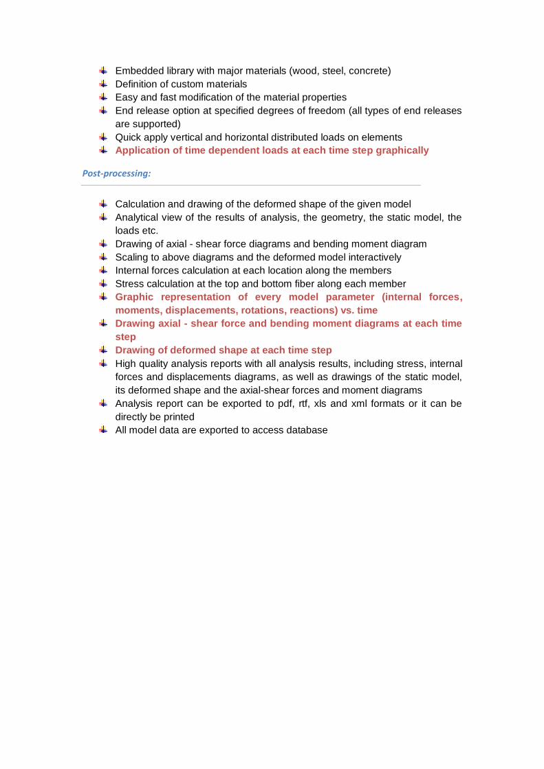
Post-processing:

Calculation and drawing of the deformed shape of the given model

Analytical view of the results of analysis, the geometry, the static model, the

loads etc.

Drawing of axial - shear force diagrams and bending moment diagram

Scaling to above diagrams and the deformed model interactively

Internal forces calculation at each location along the members

Stress calculation at the top and bottom fiber along each member

Graphic representation of every model parameter (internal forces,

moments, displacements, rotations, reactions) vs. time

Drawing axial - shear force and bending moment diagrams at each time

step

Drawing of deformed shape at each time step

High quality analysis reports with all analysis results, including stress, internal

forces and displacements diagrams, as well as drawings of the static model,

its deformed shape and the axial-shear forces and moment diagrams

Analysis report can be exported to pdf, rtf, xls and xml formats or it can be

directly be printed

All model data are exported to access database

COORDINATE SYSTEMS

Two coordinate systems are used by the program. The local one and the global one. The

global system is the same for the whole model. The local system is defined by placing its x

axis on the examined element pointing from the smaller to the greater edge node number.

This convention is respected at every reference to local and global coordinate systems.

Please note that the positive rotation convention is the counter clockwise for both

coordinate systems.

MENU DESCRIPTION

Material tab

You can define materials in this tab. Each material is defined by the following properties:

a name

the modulus of elasticity

the specific weight (this value is used only during dynamic analysis in order to

calculate the mass matrix)

the thermal coefficient, which corresponds to the axial strain when a unary

temperature change is applied to a specimen of this material

Remember that the Default material cannot be deleted.

By clicking the “From library” button, the following form is displayed which gives you the

ability to insert a pre-defined material. Steel, concrete (all grades), wood (all grades) and

custom material definition are supported.

Section tab

Sections are defined in this tab. The following properties are needed in order to define a

section:

a name

the cross section area

the moment of inertia (this inertia moment corresponds to an axis pointing into the

screen)

the section height, which is used during the calculation of the bending moments on

the frame element due to temperature differences above and below it

Remember that the Default section cannot be deleted.

By clicking the “From library” button, the following form is displayed which gives you the

ability to insert standard cross sections.

Frame element tab

In this tab, all needed data to define a frame element are given.

Geometry page

The geometry of both, starting and ending nodes, is given in this page.

You can define a frame element by clicking on the “New” button, or you can insert it

graphically by using the button of the program toolbar.

Section page

You can choose here the section of the frame element that you are about to define.

Material page

You can choose here the material of the frame element that you are about to define.

Release page

The end releases of the frame element are defined in this page. They all refer to the local

coordinate system of the frame element.

Loads page

Distributed loads on the frame element are defined in this page. They refer to the local

coordinate system of the frame element.

Node tab

As described, the nodes are generated automatically after the creation of each frame

element. In this tab, the properties of the generated nodes are given as following:

Coordinates: The coordinates of the node in the global coordinate system.

Nodal loads: The loads applied to the node in the global coordinate system.

Supports: The supports of the node.

In case of springs, the full support option should be unchecked for the

corresponding degree of freedom. The related spring constant box will then be

enabled. You have to give then the constant of the matching spring (translational or

rotational). Remember all these options refer to the global coordinate system.

Initial displacements: The initial, if any, displacements (for degrees of freedom x,y)

and rotation (for degree of freedom z) are given in this section. They are taken into

account during the static and the dynamic analysis.

Initial velocities for dynamic analysis: The initial, if any, velocities of the node are

given in this section. They are used to define the initial conditions of the model

during the dynamic analysis and they refer to the global coordinate system.

Options tab

In this tab, general program options are defined.

Units page

The measure units are defined here. You can select among a wide variety of units. The grid

size is also defined here.

Colors page

From this page, drawing colors can be customized.

Time steps page

You can define here parameters that are used during the dynamic analysis, such as the time

period and the time step number. These options affect only the dynamic analysis procedure.

By setting the current time parameter, you can see your model (both loads and results) at

the selected time.

Dynamic preferences page

The following dynamic preferences are defined in this page. They only affect the dynamic

analysis procedure:

Damping coefficient ksi: The damping coefficient that is applied to each mode as

modal damping. (equal for all modes) Zero value means no damping. Ksi mainly

depends on the material of the structure.

Number of modes to find: The desired number of nodes to be found.

Significant digits for eigenvalues: Decimal accuracy of the calculated eigenvalues.

Max. iterations for a mode: Maximum number of iterations for the estimation of a

mode.

Max. iterations for mode searches: Maximum searching iteration number to

estimate a mode.

It is suggested not to change the last three parameters in order to avoid arithmetic and

convergence problems during the dynamic analysis.

Results tab

In this tab, all analysis results regarding nodes and frame elements are presented. In case of

dynamic analysis, these results refer to the times step selected at the Time steps page in

the Options tab.

Nodes page

Nodal analysis results are presented in this section. For the selected node, the displacements

(x, y) and rotation (z) are shown, as well as the reactions, if any. In case of spring supports,

the corresponding spring reactions are shown. All these results refer to the global

coordinate system of the model.

Frame elements page

Frame elements analysis results are presented in this section. For the selected frame

element, the edge node displacements/rotation are shown, as well as the internal forces

acting on the edge nodes of the element. While all displacements and rotations refer to the

local coordinate system of the element, the internal forces are presented respecting the

classic statics convention. By clicking on the Internal forces and stresses button, you can get

the internal forces and stresses at locations along the element length.

Internal forces and stresses along member

By choosing the desired frame element and the distance from the starting node, you can get

internal element forces (axial-shear forces and bending moment) at this location. Normal

and shear stresses are also calculated at this location.

Please note that internal forces are displayed in the local coordinate system of the element.

Classic statics convention

The internal forces are presented with respect to the following coordinate system which

constitutes the classic statics convention:

Main window description

The main window of the application includes the following tab page collection. A

comprehensive description of each tab page follows.

Model tab

The static model can very easily be created from this window. The toolbar on the left can

help you during the drawing of the model interactively. A description of each toolbar button

follows:

Deformed tab

The deformed shape of the model is displayed in this tab.

Single selection

Boxed selection

Clear selection

Pan

Zoom extends

Zoom in

Zoom out

Zoom window

Draw an element

Apply element load

Apply nodal load

Apply restraints (supports)

Apply spring restraints (supports)

Clear restraints (supports)

Axial diagram tab

The axial force diagram is displayed in this tab.

Shear diagram tab

The shear force diagram is displayed in this tab.

Moment diagram tab

The moment diagram is displayed in this tab.

Modes tab

The calculated mode shapes are displayed in this tab. By clicking the Next button, more

mode shapes are displayed. The calculated period for each mode is also displayed.

Status bar description

The status bar includes the following controls:

Draw grid If selected, the grid is displayed

Snap to grid If selected, the mouse snaps to the grid points

Snap to nodes If selected, the mouse snaps to all previously created nodes

Draw element loads If selected, element loads are displayed

Draw nodal loads If selected, nodal loads are displayed

Draw supports If selected, supports are displayed

Draw reactions If selected, reactions are displayed

Show selection only If selected, only the selected elements are displayed

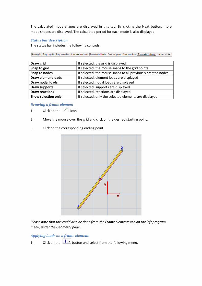
Drawing a frame element

1. Click on the icon

2. Move the mouse over the grid and click on the desired starting point.

3. Click on the corresponding ending point.

Please note that this could also be done from the Frame elements tab on the left program

menu, under the Geometry page.

Applying loads on a frame element

1. Click on the button and select from the following menu.

2. Enter a load value in the following form that will come up.

3. Click on the element you want to assign the load to.

4. The element load has been assigned to the selected element.

Please note that this could also be done from the Frame elements tab on the left program

menu, under the loads page.

Applying loads on a node

1. Click on the icon and select from the following menu.

2. Enter a load value in the following form that will come up.

3. Click on the node you want to assign the load to.

4. The element load has been assigned to the selected node.

Please note that this could also be done from the Auto generated nodes tab on the left

program menu.

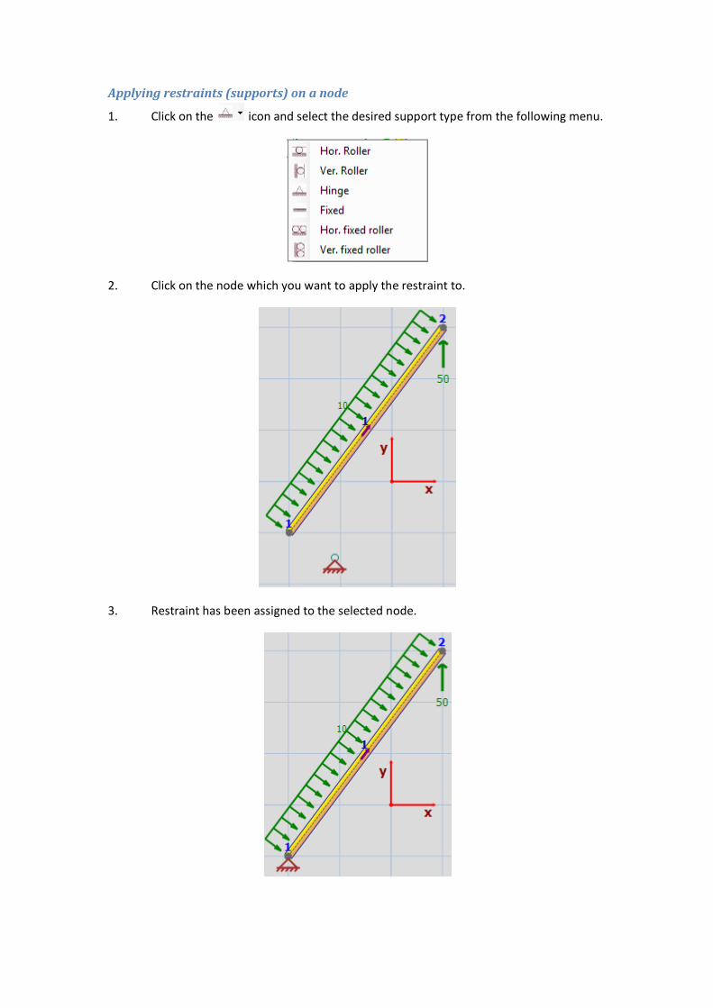
Applying restraints (supports) on a node

1. Click on the icon and select the desired support type from the following menu.

2. Click on the node which you want to apply the restraint to.

3. Restraint has been assigned to the selected node.

Please note that this could also be done from the Auto generated nodes tab on the left

program menu.

Applying spring restraints (supports) on a node

1. Click on the icon and select from the following menu.

2. Enter the spring stiffness in the following form that will come up.

3. Click on the node you want to apply the spring support to.

4. Spring support has been assigned.

Please note that this could also be done from the Auto generated nodes tab on the left

program menu.

Deleting and modifying a frame element

1. Either select the element graphically and double click on it (or right click), or select it

from the frame elements combo box in the frame elements menu on your left.

OR (double click or right click)

2. The menu with the examined frame element’s data will show, as following:

3. Click on Edit in order to enable the controls and start modifying the data, or on

Delete to delete the selected frame element.

4. Then click on OK to finish.

Modifying a node

1. Either select the node graphically and double click on it (or right click), or select it

from the nodes combo box in Auto generated nodes menu on your left.

2. The menu with the examined node’s data will show, as following:

3. Click on Edit in order to enable the controls and start modifying the data.

4. Then click on OK to finish.

Creating, modifying and deleting a material

1. Select the material from the materials combo box.

2. Click on Edit to modify its data, on Delete to delete it, or on New button to create a

new material.

3. Then click on OK to finish.

Creating, modifying and deleting a section

1. Select the section from the materials combo box.

2. Click on Edit to modify its data, on Delete to delete it, or on New button to create a

new section.

3. Then click on OK to finish.

Running static analysis

1. Make sure that the option Linear static analysis is checked under the Calculate

menu.

2. Simply click on Run analysis item or on the toolbar icon.

Running dynamic analysis

1. Make sure that the option Dynamic (Mode superposition) analysis is checked under

the Calculate menu.

2. Enter time step number in the following tab on your right.

3. Make sure that the preferences under the Dynamic Analysis tab are correct.

4. Simply click on Run analysis item or on the toolbar icon.

Applying dynamic loads

This can be done very simply following these steps:

1. Set the time step number under the Time step tab on your right.

2. Choose the time at which you want to impose a load in your model.

3. Apply the loads in your model as you would do in case of a static analysis. These

loads will be imposed only at the selected time (at 0.667 seconds)

4. Continue applying nodal and element forces for each desired time step.

Viewing results of dynamic analysis

1. Choose the time at which you want to see the results.

2. All model results will now refer to the selected time step.

Viewing graphs of dynamic analysis results

You can watch the dynamic response of the model in the whole given time span.

1. After dynamic analysis is complete, click on the icon or on the Graphics dynamic

analysis results item under the Tools menu.

2. The following form is displayed.

3. You can choose among many characteristic values (nodal displacements, reactions,

element internal forces etc) which will represent the Y axis. The X axis of the graph is the

time.

4. The graph, which is automatically created, shows the behavior of the model in the

time span in a compact form. This is of course very useful.

Creating an analysis report

1. Click on the icon.

2. A window with the created report will display.

3. By using the buttons , you can browse your report. As you can see

it contains all model data and results, as well as all diagrams regarding the deformed shape,

the internal forces diagrams (axial – shear force and bending moment) and the mode

shapes.

4. You can export the report to many formats, including .rtf (Word) and .xls (Excel) file

format by clicking on the icon.

5. The report can be printed by clicking on the icon.

In case of dynamic analysis, the results in the report refer to the latest time step.