(V) SMALL OPEN ECONOMIES LECTURES 14 & 15

• Devaluation in small open economies

• The Salter-Swan (NTGs) model

Definition of Small Open Economies: The prices of all tradable goods are determined exogenously on world markets – not just importables but exportables as well.

LECTURE 14: DEVALUATION IN SMALL OPEN ECONOMIES

Key Question: If a country is too small to affect its terms of trade (i.e., it must take prices of its X & M as given on world markets), does that mean E has no effect on TB or BP?

Answer: No. Two channels --

(1) Contractionary effects of devaluation reduce spending.

(2) Output can shift from non-traded sector to traded.

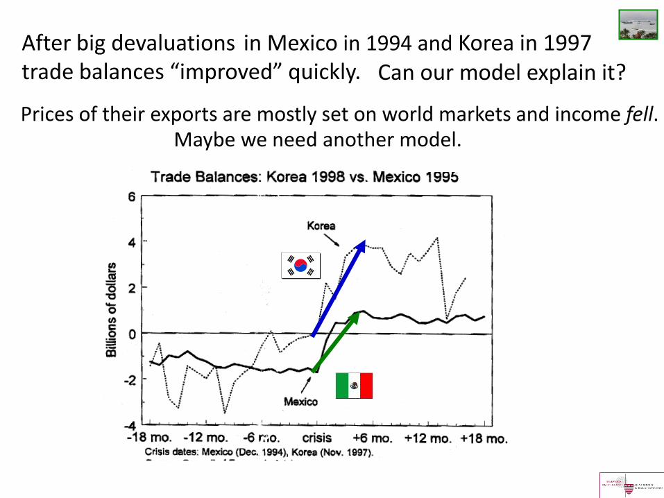
After big devaluations in Mexico in 1994 and Korea in 1997 trade balances “improved” quickly.

Prices of their exports are mostly set on world markets and income fell.

Can our model explain it?

Maybe we need another model.

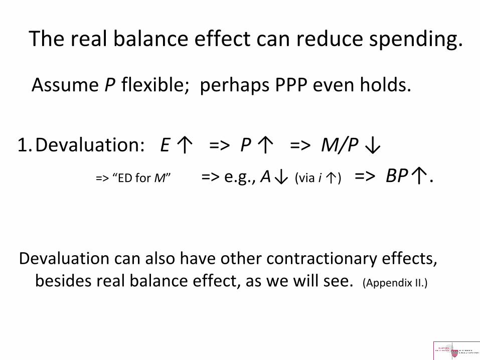
The real balance effect can reduce spending.

Assume P flexible; perhaps PPP even holds.

1.Devaluation: E ↑ => P ↑ => M/P ↓

=> “ED for M” => e.g., A ↓ (via i ↑) => BP ↑.

Devaluation can also have other contractionary effects, besides real balance effect, as we will see. (Appendix II.)

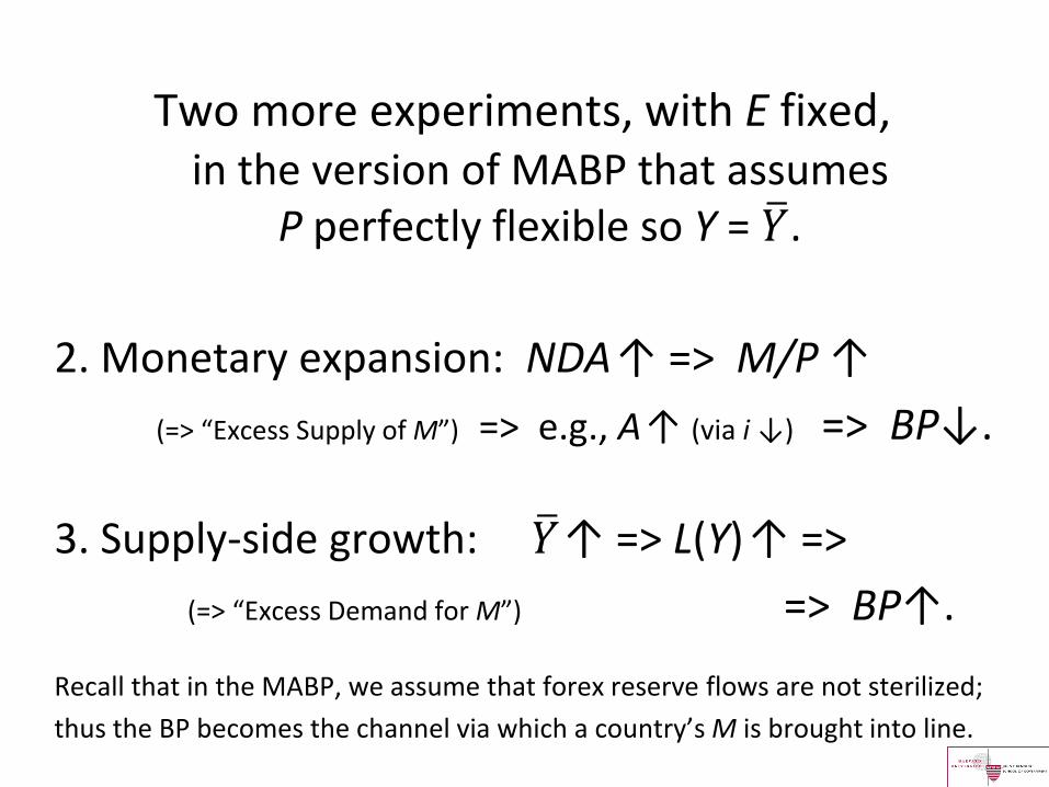
Two more experiments, with E fixed,

2. Monetary expansion: NDA ↑ => M/P ↑

(=> “Excess Supply of M”) => e.g., A ↑ (via i ↓) => BP↓.

3. Supply-side growth: 𝑌 ↑ => L(Y) ↑ =>

(=> “Excess Demand for M”) => BP↑.

Recall that in the MABP, we assume that forex reserve flows are not sterilized;

thus the BP becomes the channel via which a country’s M is brought into line.

in the version of MABP that assumes P perfectly flexible so Y = 𝑌 .

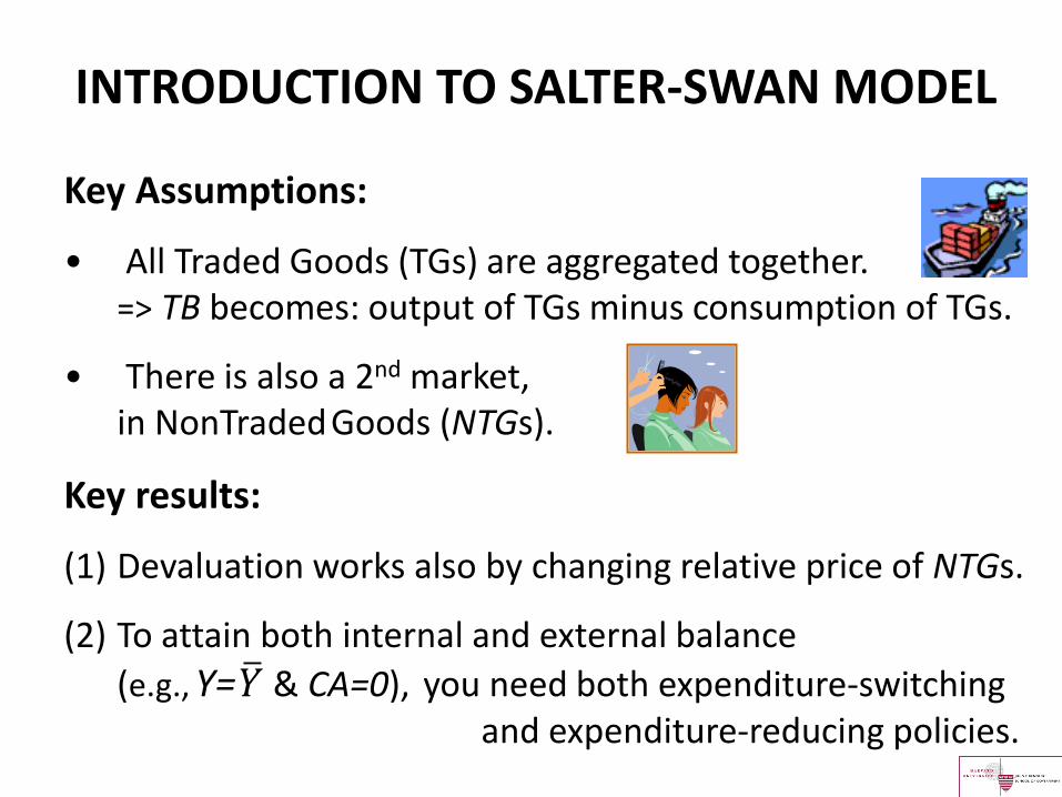
INTRODUCTION TO SALTER-SWAN MODEL

Key Assumptions:

• All Traded Goods (TGs) are aggregated together. => TB becomes: output of TGs minus consumption of TGs.

• There is also a 2nd market, in NonTraded Goods (NTGs).

Key results:

(1) Devaluation works also by changing relative price of NTGs.

(2) To attain both internal and external balance

(e.g., Y= 𝑌 & CA=0), you need both expenditure-switching and expenditure-reducing policies.

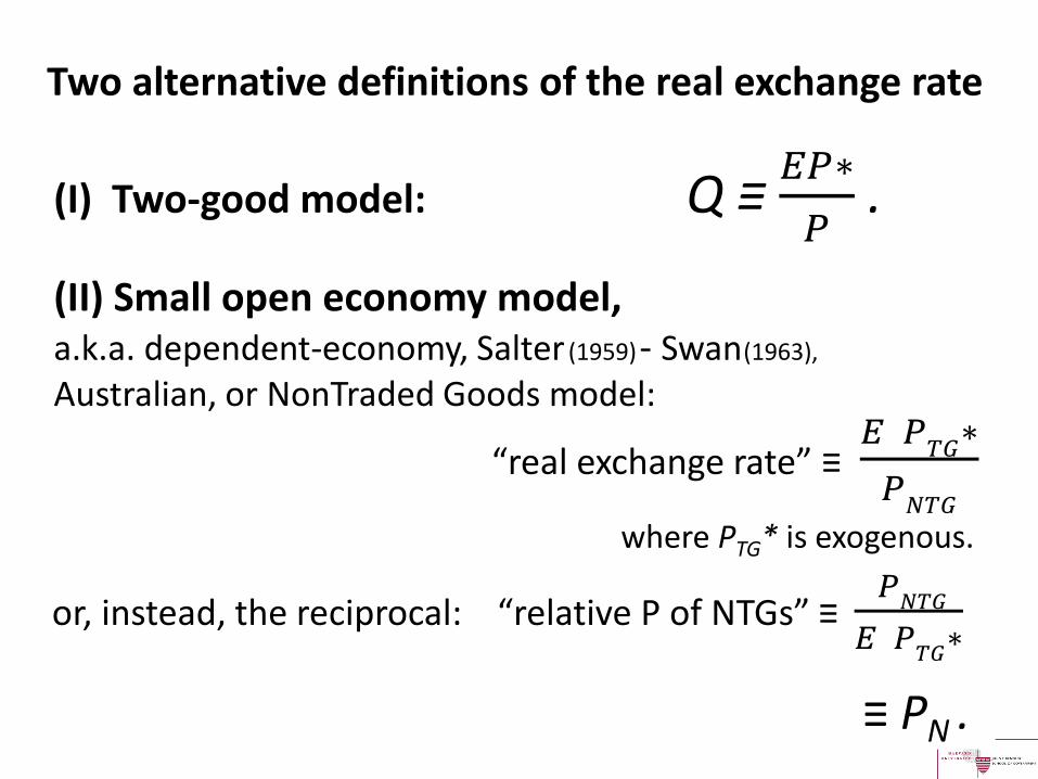
Two alternative definitions of the real exchange rate

(I) Two-good model: Q ≡ 𝐸𝑃∗

𝑃 .

(II) Small open economy model, a.k.a. dependent-economy, Salter (1959) - Swan (1963),

Australian, or NonTraded Goods model:

“real exchange rate” ≡ 𝐸 𝑃

𝑇𝐺∗

𝑃𝑁𝑇𝐺

or, instead, the reciprocal: “relative P of NTGs” ≡ 𝑃

𝑁𝑇𝐺

𝐸 𝑃𝑇𝐺

∗

≡ PN .

where PTG* is exogenous.

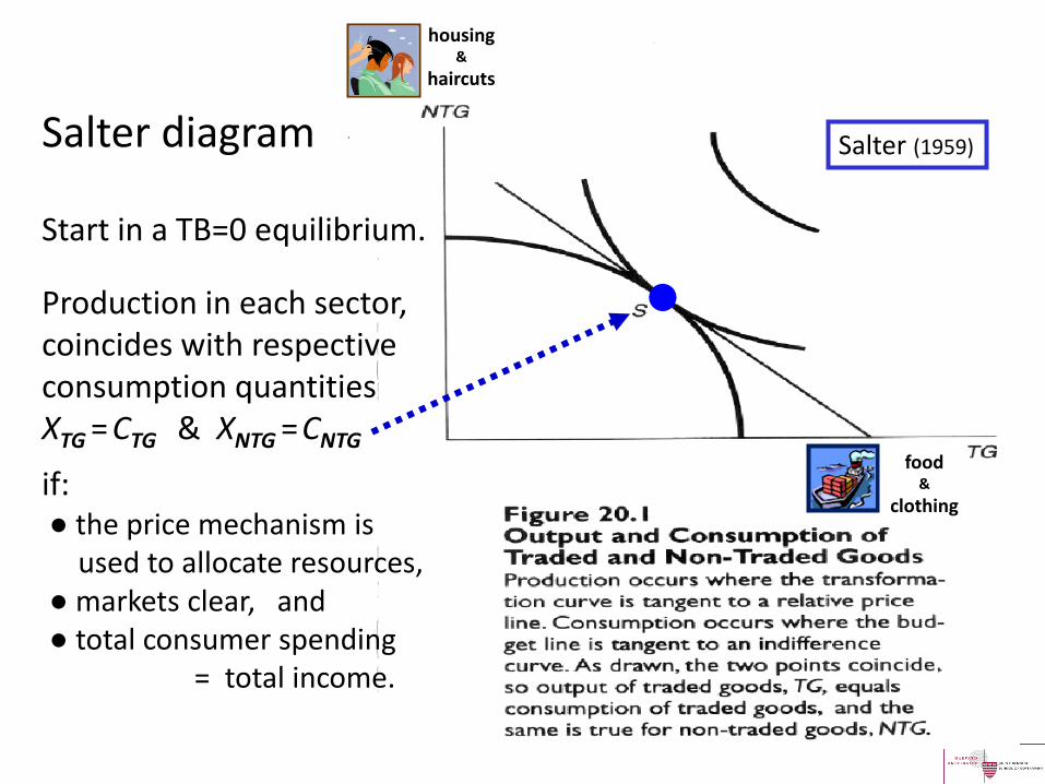
Salter diagram

Start in a TB=0 equilibrium.

Production in each sector, coincides with respective consumption quantities XTG = CTG & XNTG = CNTG

if: ● the price mechanism is used to allocate resources, ● markets clear, and ● total consumer spending = total income.

Salter (1959)

●

housing &

haircuts

food &

clothing

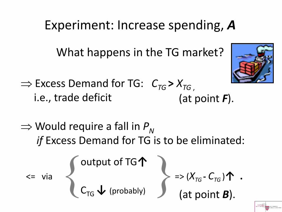
Experiment: Increase spending, A

What happens in the TG market?

Excess Demand for TG: CTG > XTG , i.e., trade deficit

Would require a fall in PN

if Excess Demand for TG is to be eliminated:

output of TG↑ <= via => (XTG - CTG )↑ .

CTG ↓ (probably) { }

(at point F).

(at point B).

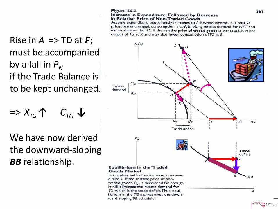
Rise in A => TD at F ; must be accompanied by a fall in PN if the Trade Balance is to be kept unchanged.

=> CTG ↓ We have now derived the downward-sloping BB relationship.

XTG ↑

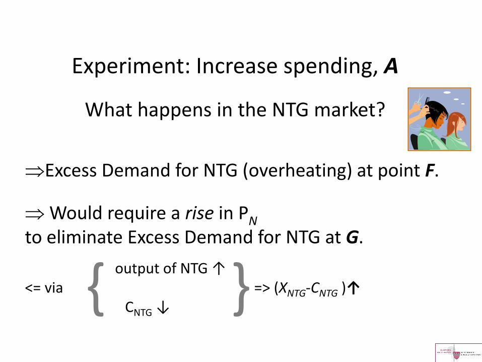
Experiment: Increase spending, A

Excess Demand for NTG (overheating) at point F.

Would require a rise in PN to eliminate Excess Demand for NTG at G.

output of NTG ↑ <= via => (XNTG-CNTG )↑ CNTG ↓

{ }

What happens in the NTG market?

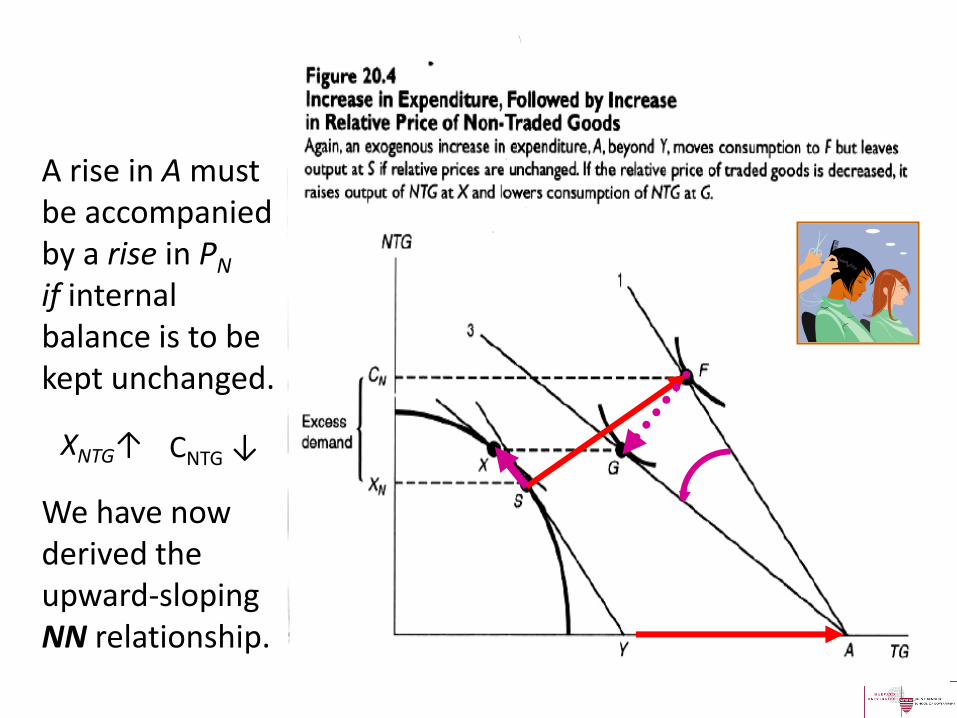
A rise in A must be accompanied by a rise in PN if internal balance is to be kept unchanged.

We have now derived the upward-sloping NN relationship.

CNTG ↓ XNTG↑

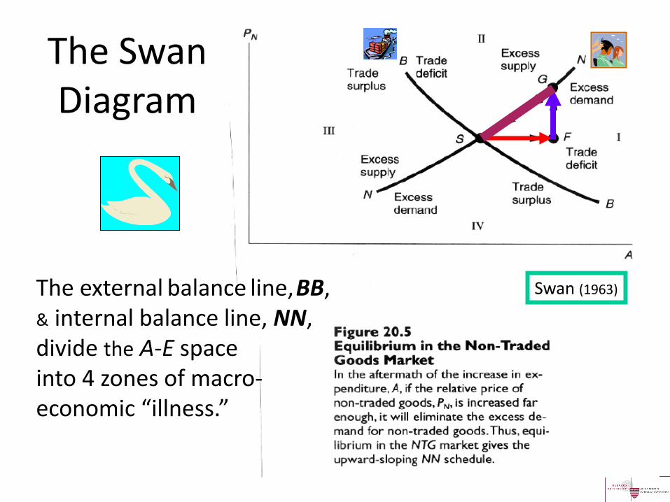
The Swan Diagram

The external balance line, BB, & internal balance line, NN, divide the A-E space into 4 zones of macro- economic “illness.”

Swan (1963)

Swan Diagram, continued

The Tinbergen-Meade principle of targets & instruments

To attain two goals -- internal and external balance -- you need two independent policy instruments:

expenditure-switching policies (exchange rate)

and expenditure-reducing policies (fiscal or monetary contraction).

15

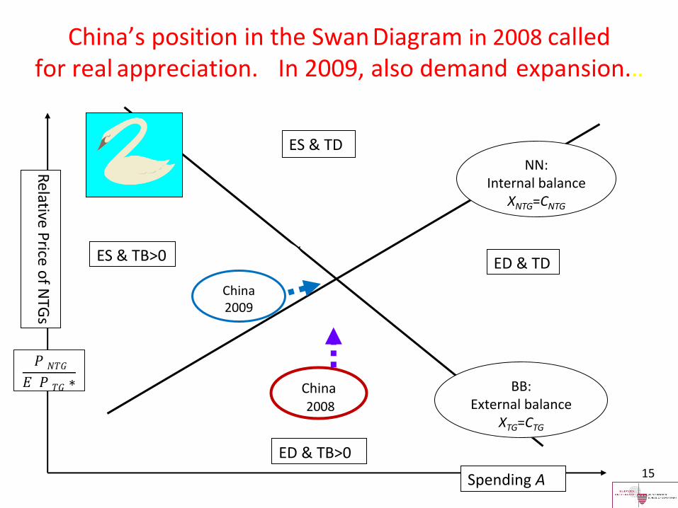
China’s position in the Swan Diagram in 2008 called for real appreciation. .

Relative P

rice of N

TGs

ED & TD

ES & TD

ES & TB>0

China 2008

BB: External balance

XTG=CTG

China 2002

ED & TB>0

Spending A

China 2009

NN: Internal balance

XNTG=CNTG

𝑃 𝑁𝑇𝐺

𝐸 𝑃 𝑇𝐺 ∗

In 2009, also demand expansion..

Two policy experiments

• (1) Fall in Demand: A

• => recession at point H in fig. 20.6.

If PN is sticky & exchange rate fixed, downward adjustment to point E may be slow & painful.

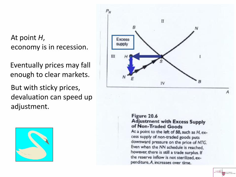
At point H, economy is in recession.

Eventually prices may fall enough to clear markets.

But with sticky prices, devaluation can speed up adjustment.

Second policy experiment

(2) Devaluation: E

Improves TB in two ways:

(i) Real balance effect, reduces spending.

(ii) Fall in PNTG /PTG , switches spending out of TG, & switches supply into TG (at E).

Appendix I: Rudiger Dornbusch, AER (1973)

“Devaluation, Money & Nontraded Goods”

Combines NTG model , with MABP

Two automatic mechanisms of adjustment:

(i) PNTG flexible => always on NN; PN rises instantly in response to ED.

(ii) reserve flows not sterilized; Money adjusts in response to TD.

E.g., two experiments 1. NDA => jump to point G. (Fig. 20.5)

2. E => jump to point E. (Fig. 20.6) In each case, over time, reserve flows gradually bring

the economy back to S (following the sequence of arrows).

Two prominent explanations:

• High interest rates raise default probability.

The IMF may not have sufficiently realized this – according to Furman & Stiglitz; and Radelet & Sachs; both in BPEA (1998).

• Devaluation is contractionary: many possible channels, including real balance effect & balance-sheet effect.

Appendix II: CONTRACTIONARY EFFECTS OF DEVALUATION

Why were the real effects of the 1997-98 East Asia currency crisis so severe?

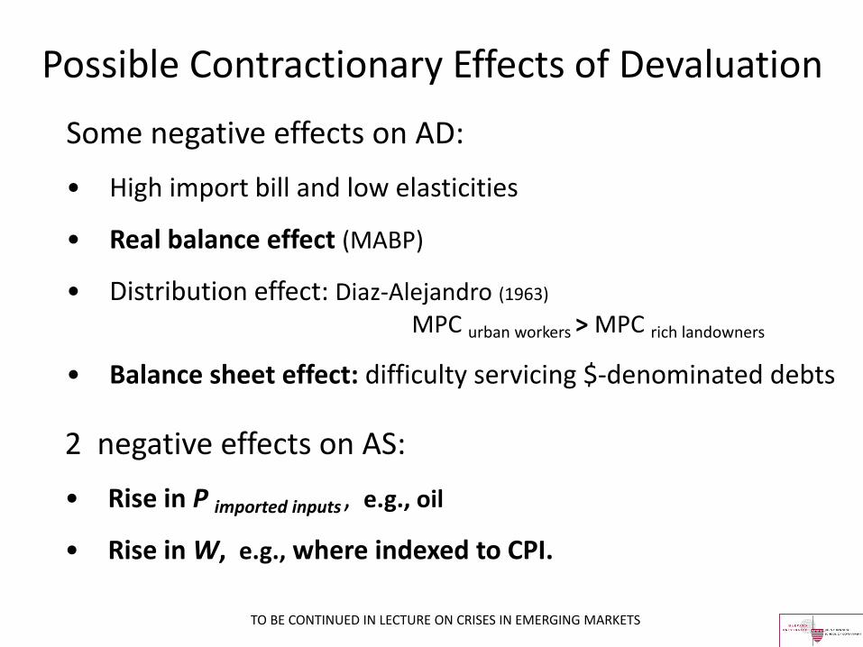
Some negative effects on AD:

• High import bill and low elasticities

• Real balance effect (MABP)

• Distribution effect: Diaz-Alejandro (1963)

MPC urban workers > MPC rich landowners

• Balance sheet effect: difficulty servicing $-denominated debts

Possible Contractionary Effects of Devaluation

2 negative effects on AS:

• Rise in P imported inputs , e.g., oil

• Rise in W, e.g., where indexed to CPI.

TO BE CONTINUED IN LECTURE ON CRISES IN EMERGING MARKETS

API-120 - Prof. J.Frankel

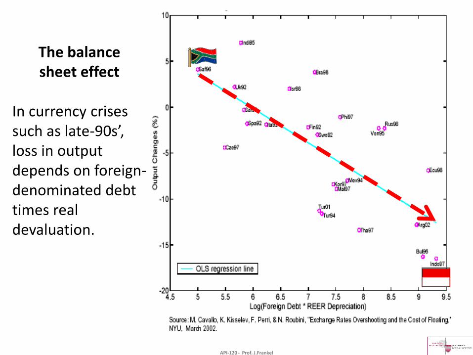
The balance sheet effect

In currency crises such as late-90s’, loss in output depends on foreign-denominated debt times real devaluation.