V. EMPIRICAL RESULTS INDIA 632 0.0003 0.0609 - … · malaysia 646 - 0.0001 0.0288 - 0.0536 0.0006...

~ 1 ~

V. EMPIRICAL RESULTS

V.1. DESCRIPTIVE STATISTICS

For each of the market returns, the descriptive statistics and their corresponding

standard errors and test statistics are calculated using Excel. The results for the first and

second moments for total observations are arranged on regional classification and

presented in the following table:

SIZE MEAN MAX MIN MEDIAN STD. DEV

EGYPT 495 0.0004- 0.0240 0.0538- 0.0010 0.0104

ISRAEL 546 0.0002 0.0340 0.0566- 0.0012 0.0114

S. AFRICA 675 0.0001- 0.1003 0.1138- 0.0010 0.0189

ARGENTINA 647 0.0009- 0.0653 0.1052- 0.0005 0.0157

BRAZIL 733 0.0008 0.1231 0.1124- 0.0019 0.0223

CANADA 698 0.0005- 0.0815 0.0892- 0.0009 0.0147

CHILE 662 0.0004 0.1060 0.0698- 0.0019 0.0133

MEXICO 669 0.0000 0.0850 0.0860- 0.0011 0.0173

UNITED STATES 733 0.0003- 0.0689 0.0689- 0.0003 0.0122

AUSTRALIA 712 0.0001- 0.0831 0.0804- 0.0013 0.0157

CHINA 657 0.0016 0.0865 0.0548- 0.0029 0.0153

HONG KONG 651 0.0002 0.0759 0.1049- 0.0010 0.0149

INDONESIA 634 0.0000 0.0662 0.1033- 0.0017 0.0157

INDIA 632 0.0003 0.0609 0.0806- 0.0017 0.0166

JAPAN 632 0.0005- 0.0786 0.0591- 0.0000 0.0121

MALAYSIA 646 0.0001- 0.0288 0.0536- 0.0006 0.0090

NEW ZEALAND 688 0.0005- 0.0569 0.0548- 0.0004 0.0121

PHILIPPINES 649 0.0000- 0.0508 0.0776- 0.0015 0.0145

SINGAPORE 678 0.0004- 0.0526 0.0639- 0.0006 0.0123

S. KOREA 644 0.0006 0.1378 0.1139- 0.0018 0.0189

TAIWAN 650 0.0002- 0.0565 0.0454- 0.0011 0.0123

THAILAND 624 0.0003- 0.0575 0.0874- 0.0001 0.0124

AFRICA

AMERICA

ASIA

~ 2 ~


EURO AREA 717 0.0002- 0.0727 0.0701- 0.0003 0.0140

AUSTRIA 662 0.0006- 0.1097 0.0821- 0.0008 0.0178

DENMARK 693 0.0004- 0.0757 0.0682- 0.0005 0.0147

FRANCE 718 0.0002- 0.0767 0.0715- 0.0006 0.0142

GERMANY 714 0.0001 0.0755 0.0649- 0.0011 0.0139

NETHERLANDS 715 0.0004- 0.0717 0.0740- 0.0005 0.0147

RUSSIA 647 0.0000 0.1484 0.1310- 0.0011 0.0219

SPAIN 711 0.0001 0.0733 0.0685- 0.0011 0.0139

SWEDEN 689 0.0001- 0.0852 0.0674- 0.0012 0.0165

SWITZERLAND 693 0.0003- 0.0760 0.0577- 0.0003 0.0114

UNITED KINGDOM 711 0.0005- 0.0785 0.0709- 0.0003 0.0139

EUROPE

Table 1. Descriptive Statistics of the Full Sample Market Returns based on Regional Classification

From the table above it can be seen that several economies have positive average

returns: Israel, Brazil, Chile, Mexico, China, Hong Kong, Indonesia, India, South Korea,

Germany, and Spain. As for the rest of the markets, they reported negative average return.

Nevertheless, the median for all markets are uniformly positive. It signifies the presence of

extreme large values in the distribution. As for the variation around the mean return,

Russia shows the highest volatility during the time period considered. Volatility is highest in

South Africa, Brazil, South Korea and Russia for Africa, America, Asia, and Europe region,

respectively. Since the samples are divided into two sub-groups, the statistics of each

period are also determined and summarized as follows1:

1 Since the lag order p = 3, observation for tranquil period starts at t = p + 1 = 4

~ 3 ~


EGYPT 472 0.0002- 0.0240 0.0538- 0.0010 0.0101

ISRAEL 546 0.0002 0.0340 0.0566- 0.0011 0.0114

S. AFRICA 675 0.0002- 0.1003 0.1138- 0.0009 0.0190

ARGENTINA 554 0.0004- 0.0589 0.0524- 0.0006 0.0117

BRAZIL 623 0.0012 0.0842 0.0774- 0.0020 0.0172

CANADA 595 0.0001 0.0556 0.0525- 0.0010 0.0099

CHILE 559 0.0008 0.0354 0.0415- 0.0018 0.0102

MEXICO 568 0.0006 0.0582 0.0412- 0.0017 0.0123

UNITED STATES 626 0.0000 0.0490 0.0459- 0.0005 0.0077

AUSTRALIA 605 0.0004 0.0720 0.0552- 0.0014 0.0116

CHINA 556 0.0017 0.0865 0.0548- 0.0029 0.0151

HONG KONG 551 0.0006 0.0565 0.0417- 0.0012 0.0113

INDONESIA 547 0.0007 0.0537 0.0678- 0.0023 0.0135

INDIA 548 0.0010 0.0534 0.0575- 0.0021 0.0144

JAPAN 543 0.0001- 0.0295 0.0282- 0.0001 0.0089

MALAYSIA 558 0.0002 0.0276 0.0536- 0.0008 0.0084

NEW ZEALAND 585 0.0000- 0.0346 0.0477- 0.0005 0.0089

PHILIPPINES 546 0.0004 0.0475 0.0572- 0.0018 0.0126

SINGAPORE 578 0.0004 0.0344 0.0407- 0.0010 0.0098

S. KOREA 541 0.0009 0.0407 0.0355- 0.0019 0.0109

TAIWAN 552 0.0000- 0.0444 0.0454- 0.0011 0.0104

THAILAND 526 0.0003 0.0373 0.0874- 0.0003 0.0108

EURO AREA 608 0.0002 0.0467 0.0391- 0.0003 0.0090

AUSTRIA 560 0.0001- 0.0679 0.0649- 0.0008 0.0120

DENMARK 586 0.0003 0.0463 0.0559- 0.0011 0.0102

FRANCE 609 0.0002 0.0486 0.0404- 0.0007 0.0094

GERMANY 607 0.0005 0.0356 0.0383- 0.0011 0.0089

NETHERLANDS 607 0.0001- 0.0432 0.0712- 0.0006 0.0099

RUSSIA 553 0.0003 0.1172 0.0893- 0.0011 0.0158

SPAIN 604 0.0006 0.0486 0.0368- 0.0014 0.0090

SWEDEN 584 0.0002 0.0509 0.0535- 0.0013 0.0112

SWITZERLAND 586 0.0001 0.0324 0.0356- 0.0004 0.0078

UNITED KINGDOM 602 0.0000- 0.0514 0.0467- 0.0005 0.0091

AFRICA

AMERICA

ASIA

EUROPE

Table 2. Descriptive Statistics of Market Returns for Tranquil Period

~ 4 ~

SIZE MEAN MAX MIN MEDIAN STDEV

EGYPT 20 0.0057- 0.0121 0.0340 0.1003 0.0153

ISRAEL 35 0.0010- 0.0445- 0.0566- 0.1138- 0.0220

S. AFRICA 104 0.0016- 0.0035- 0.0034 0.0026- 0.0353

ARGENTINA 90 0.0048- 0.0653 0.1052- 0.0033- 0.0304

BRAZIL 107 0.0017- 0.1231 0.1124- 0.0003- 0.0411

CANADA 100 0.0041- 0.0815 0.0892- 0.0029- 0.0302

CHILE 100 0.0018- 0.1060 0.0698- 0.0024 0.0243

MEXICO 98 0.0033- 0.0850 0.0860- 0.0051- 0.0341

UNITED STATES 107 0.0022- 0.0689 0.0689- 0.0028- 0.0261

AUSTRALIA 104 0.0032- 0.0831 0.0804- 0.0016- 0.0302

CHINA 98 0.0011 0.0450 0.0424- 0.0003 0.0170

HONG KONG 97 0.0020- 0.0759 0.1049- 0.0000- 0.0278

INDONESIA 84 0.0047- 0.0662 0.1033- 0.0039- 0.0256

INDIA 81 0.0040- 0.0609 0.0806- 0.0025- 0.0272

JAPAN 86 0.0033- 0.0786 0.0591- 0.0060- 0.0239

S. KOREA 100 0.0011- 0.1378 0.1139- 0.0023- 0.0409

MALAYSIA 85 0.0017- 0.0288 0.0300- 0.0030- 0.0123

NEW ZEALAND 100 0.0031- 0.0569 0.0548- 0.0008- 0.0232

PHILIPPINES 100 0.0023- 0.0508 0.0776- 0.0002- 0.0221

SINGAPORE 97 0.0049- 0.0526 0.0639- 0.0039- 0.0214

TAIWAN 95 0.0013- 0.0565 0.0418- 0.0009 0.0199

THAILAND 95 0.0038- 0.0575 0.0579- 0.0032- 0.0188

EURO AREA 106 0.0025- 0.0727 0.0701- 0.0021- 0.0292

AUSTRIA 99 0.0035- 0.1097 0.0821- 0.0042- 0.0362

DENMARK 104 0.0041- 0.0757 0.0682- 0.0033- 0.0290

FRANCE 106 0.0023- 0.0767 0.0715- 0.0020- 0.0292

GERMANY 104 0.0022- 0.0755 0.0649- 0.0020- 0.0294

NETHERLANDS 105 0.0025- 0.0717 0.0740- 0.0016- 0.0301

RUSSIA 91 0.0020- 0.1484 0.1310- 0.0008 0.0435

SPAIN 104 0.0026- 0.0733 0.0685- 0.0031- 0.0290

SWEDEN 102 0.0026- 0.0852 0.0674- 0.0019- 0.0290

SWITZERLAND 104 0.0027- 0.0760 0.0577- 0.0020- 0.0228

UNITED KINGDOM 106 0.0031- 0.0785 0.0709- 0.0021- 0.0286

AFRICA

AMERICA

EUROPE

ASIA

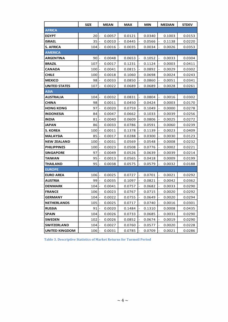
Table 3. Descriptive Statistics of Market Returns for Turmoil Period

~ 5 ~

In tranquil times, there are only a handful of markets exhibit negative mean

returns: Egypt, South Africa, Argentina, Japan, New Zealand, Taiwan, Austria, the

Netherlands and United Kingdom. However, during the turmoil period, all markets

uniformly reported negative average return. The opposite direction is observed in the

variance of each return, the volatility is significantly higher during the turmoil period. This

pattern is omnipresent for all markets under investigation.

In order to deduce information from the distribution of the market returns, these

statistics are analysed using parametric tests described in details in the preceding chapter.

The standard error and t-statistic for each distribution parameters mentioned above are

calculated only for the full sample. The results are arranged based on regional

classification:

~ 6 ~

STAT SE t STAT SE t STAT SE t

EGYPT 0.00- 0.00 0.87- 1.07- 0.11 9.72- 2.48 0.22 2.37-

ISRAEL 0.00 0.00 0.51 1.00- 0.10 9.57- 3.40 0.21 1.88

S. AFRICA 0.00- 0.00 0.17- 0.02 0.09 0.22 4.67 0.19 8.87

ARGENTINA 0.00- 0.00 1.51- 0.85- 0.10 8.79- 6.10 0.19 16.10

BRAZIL 0.00 0.00 0.92 0.13- 0.09 1.42- 5.05 0.18 11.34

CANADA 0.00- 0.00 0.88- 0.62- 0.09 6.64- 7.96 0.19 26.75

CHILE 0.00 0.00 0.83 0.22- 0.10 2.36- 9.05 0.19 31.80

MEXICO 0.00 0.00 0.05 0.21- 0.09 2.26- 5.06 0.19 10.85

UNITED STATES 0.00- 0.00 0.67- 0.30- 0.09 3.37- 7.04 0.18 22.34

AUSTRALIA 0.00 0.00 0.16- 0.02 0.10 3.86- 1.89 0.19 11.47

CHINA 0.00 0.00 2.68 0.12- 0.10 0.16 6.78 0.19 5.82-

HONG KONG 0.00 0.00 0.30 1.10- 0.10 1.23- 6.45 0.19 19.71

INDONESIA 0.00 0.00 0.01 0.52- 0.10 11.27- 2.22 0.19 17.73

INDIA 0.00- 0.00 0.51 0.15- 0.10 5.35- 5.44 0.19 4.02-

JAPAN 0.00- 0.00 1.05- 0.60- 0.10 1.52- 3.42 0.19 12.52

MALAYSIA 0.00- 0.00 0.17- 0.56- 0.09 6.22- 3.98 0.19 2.17

NEW ZEALAND 0.00- 0.00 1.07- 0.58- 0.10 6.03- 3.19 0.19 5.25

PHILIPPINES 0.00- 0.00 0.03- 0.49- 0.09 6.06- 3.52 0.19 0.96

SINGAPORE 0.00 0.00 0.83- 0.15 0.10 5.17- 14.44 0.19 2.77

S. KOREA 0.00- 0.00 0.81 0.26- 0.10 1.60 1.62 0.19 59.28

TAIWAN 0.00- 0.00 0.37- 0.76- 0.10 2.69- 6.80 0.20 7.20-

THAILAND 0.00- 0.00 0.63- 0.76- 0.10 7.80- 6.80 0.20 19.39

EURO AREA 0.00- 0.00 0.35- 0.01 0.09 0.07 5.53 0.18 13.84

AUSTRIA 0.00- 0.00 0.89- 0.04- 0.10 0.44- 6.78 0.19 19.87

DENMARK 0.00- 0.00 0.66- 0.38- 0.09 4.05- 5.95 0.19 15.83

FRANCE 0.00- 0.00 0.33- 0.19 0.09 2.05 6.08 0.18 16.84

GERMANY 0.00 0.00 0.18 0.07 0.09 0.72 5.58 0.18 14.07

NETHERLANDS 0.00- 0.00 0.75- 0.33- 0.09 3.65- 5.84 0.18 15.51

RUSSIA 0.00 0.00 0.03 0.13- 0.10 1.38- 11.47 0.19 43.97

SPAIN 0.00 0.00 0.22 0.11- 0.09 1.22- 6.18 0.18 17.32

SWEDEN 0.00- 0.00 0.09- 0.18 0.09 1.92 4.37 0.19 7.33

SWITZERLAND 0.00- 0.00 0.70- 0.07- 0.09 0.73- 6.22 0.19 17.32

UNITED KINGDOM 0.00- 0.00 0.96- 0.10 0.09 1.03 7.31 0.18 23.43

AFRICA

AFRICA

ASIA

EUROPE

KURTOSISMEAN SKEWNESS

Table 4. Distribution Parameter Test Statistics based on Regional Classification

At level of significance α = 5% the null hypothesis of the sample means cannot be

rejected for almost all stock markets considered in this study. The parametric test

~ 7 ~

conducted on the sample mean indicates the estimated arithmetic mean is significant for

most of the countries investigated, except for the Shanghai SE in China. The t-statistic

indicates that we reject the null hypothesis for this market.

The second parametric test is carried out on the skewness coefficient. The results

of the test for skewness indicate that the distribution of international equity market

encompasses different shapes. Some estimated skewness coefficients are not significantly

different from zero; this is the case for market returns in South Africa, Brazil, China, Hong

Kong, Japan, South Korea, Euro Area, Austria, Germany, Russia, Spain, Sweden, Switzerland

and United Kingdom. As for the sample from Egypt, Israel, Argentina, Canada, Chile,

Mexico, United States, Australia, Indonesia, India, Malaysia, New Zealand, Philippines,

Singapore, Taiwan, Thailand, Denmark and the Netherlands, the null hypothesis is rejected

and the estimated negative coefficient of skewness for each of these market is statistically

significant. It is worth nothing that Indonesia has the highest negative skewness coefficient.

On the other hand, only one market shows a significant positively-skewed distribution, i.e.

the CAC 40 in France.

Random variables with a negative skewness coefficient is said to have a distribution

that is distorted to the left, i.e. left-skewed, due to the presence of extremely small values

(Berenson, Levine, & Krehbiel, 2009). In other words, this distribution is characterized by

higher probability for values to be lower than the expected value that it is for value to fall

above the mean (Hamilton, 1994). Since most of the values are in the upper proportion of

the distribution, the mean value of this distribution is smaller than its median (Berenson,

Levine, & Krehbiel, 2009).

Contrarily, a positive value of skewness coefficient indicates right-skewness which

means that the mean are larger than the median, i.e. most of the values are in the lower

~ 8 ~

proportion of the distribution (Berenson, Levine, & Krehbiel, 2009). The result of the t-test

indicates the presence of extreme positive values, i.e. higher returns than expected, in

France market.

The third test implemented in this study is the test of excess kurtosis. Test statistics

for kurtosis coefficient reveal that most of the returns in this study have significant positive

excess kurtosis (Kr > 3). This type of distribution is said to have high peak and heavy tails,

and often referred to as a leptokurtic distribution (Tsay, 2005). This type of distribution

implies that the tails of its support have more mass than a Gaussian distribution with the

same variance does (Hamilton, 1994; Tsay, 2005). In practice, this means that a random

sample from such a distribution tends to contain more extreme values from the upper or

the lower side of the mean (Tsay, 2005).

Only two countries are found to have kurtosis coefficient not significantly different

from three, i.e. Israel and the Philippines. Therefore, it can be conjectured that the peak

and tails of the distribution from the two markets are approaching those of normal

distribution. On the other hand, some countries, namely Egypt, China, India, and Taiwan,

are found to have kurtosis coefficient to be significantly less than three. Distribution with

negative excess kurtosis has short tails and is called a platykurtic distribution (Tsay, 2005).

This type of distribution will be less peaked in the mean, have thinner tails and more of the

distribution in the shoulders than a normal distribution (Brooks, 2008).

Countries in this study are also grouped according to their income level (The World

Bank, 2010). Classifying countries based on their economic development provides another

perspective on the distribution of market returns. Therefore the results are re-arranged as:

~ 9 ~

COUNTRY SKEWNESS KURTOSIS COUNTRY SKEWNESS KURTOSIS

CHINA NON PLATY CANADA NEGATIVE LEPTO

EGYPT NEGATIVE PLATY DENMARK NEGATIVE LEPTO

INDONESIA NEGATIVE LEPTO EURO AREA NON LEPTO

INDIA NEGATIVE PLATY FRANCE POSITIVE LEPTO

PHILIPPINES NEGATIVE NON GERMANY NON LEPTO

THAILAND NEGATIVE LEPTO HONG KONG NON LEPTO

ISRAEL NEGATIVE NON

ARGENTINA NEGATIVE LEPTO JAPAN NON LEPTO

BRAZIL NON LEPTO NETHERLANDS NEGATIVE LEPTO

CHILE NEGATIVE LEPTO NEW ZEALAND NEGATIVE LEPTO

MALAYSIA NEGATIVE LEPTO SINGAPORE NEGATIVE LEPTO

MEXICO NEGATIVE LEPTO S. KOREA NON LEPTO

RUSSIA NON LEPTO SPAIN NON LEPTO

S. AFRICA NON LEPTO SWEDEN NON LEPTO

SWITZERLAND NON LEPTO

AUSTRALIA NEGATIVE LEPTO UNITED KINGDOM NON LEPTO

AUSTRIA NON LEPTO UNITED STATES NEGATIVE LEPTO

LOWER-MIDDLE INCOME

UPPER-MIDDLE INCOME

HIGH INCOME

HIGH INCOME

Table 5. Distribution Parameters based on Income-Level Classification2

The results in Table 6. indicate that all of the countries in lower-middle income

group, except for China, have significant negatively-skewed distribution. For other income

levels the results indicate a rather heterogeneous picture: some markets have left-skewed

distribution; some do not have significant skewness in their distribution. One market in

high-income group exhibits positively-skewed distribution. However, the analysis of

kurtosis coefficients when countries are grouped based on their economic development

indicates a somewhat regular pattern. Other than Israel, all of the countries in the upper-

middle and high income groups have significant leptokurtic distribution. Meanwhile only

two countries in the lower-middle income group exhibit significant excess kurtosis. These

statistics appear to be in contrary to the results obtained by another study in international

stock markets over the period of 1994 - 2005 (Evans & McMillan, 2009) in which they

suggested that excess kurtosis is more noticeable for developing economies.

2 Taiwan is excluded from the list based on income-level classification because it is not listed on the

World Bank website

~ 10 ~

V.2. NORMALITY TEST

EGYPT 100.19 NEW ZEALAND 63.90

ISRAEL 95.05 PHILIPPINES 37.69

S. AFRICA 78.81 SINGAPORE 34.37

S. KOREA 3,516.51

ARGENTINA 336.49 TAIWAN 59.10

BRAZIL 130.54 THAILAND 436.77

CANADA 759.85

CHILE 1,016.71 EURO AREA 191.54

MEXICO 122.87 AUSTRIA 394.88

UNITED STATES 510.26 DENMARK 267.14

FRANCE 287.79

AUSTRALIA 146.56 GERMANY 198.35

CHINA 33.95 NETHERLANDS 253.96

HONG KONG 389.89 RUSSIA 1,935.69

INDONESIA 441.17 SPAIN 301.52

INDIA 44.86 SWEDEN 57.39

JAPAN 159.04 SWITZERLAND 300.46

MALAYSIA 43.42 UNITED KINGDOM 550.20

AFRICA ASIA

AMERICA

EUROPE

ASIA

Table 6. Normality Test of Market Returns

From the results of the JB statistics tabulated in Table 7, it can be concluded that all

of stock returns in this study are found to have a distribution which is significantly different

from normal distribution, with South Korea have the highest JB statistic. Non-normality in

financial data could correspond to a one-off or extreme events that are unlikely to be

repeated and the information content of which is deemed of no relevance for the data as a

whole (e.g. stock market crashes, financial panics, etc) or it could also arise from certain

types of heteroscedasticity (Brooks, 2008) whereas in the latter case the non-normality is

intrinsic to all of the data and outlier removal would not make the residuals of such a

model normal.

No conclusion can be made regarding the source of the non-normality of market

returns examined in this study. However, it is worth noting that a leptokurtic distribution

~ 11 ~

with fatter tails and is more peaked at the mean than a normally distributed random

variable with the same mean and variance is far more likely to characterize financial time

series and the residuals from a financial time series model (Tsay, 2005; Brooks, 2008). The

larger the deviation from normality for market returns, the more volatile they are, i.e.

extreme values can be observed with relatively higher frequency.

It is suggested that positive kurtosis and negative skewness can be attributed to

not only the inherent heteroscedasticity of market returns, i.e. time-varying variance, but

also to the non-stationarity of their population mean, as appear to be the case of this study

(Fama, 1965; Stokie, 1982). As the result of the unconditional heteroscedasticity, even for a

very large sample the variability of the sample variance will not tend to dampen nearly as

much as would be expected with a Gaussian process (Fama, 1965). Nevertheless, due to

the scope of this study, implications of the non-normality in market returns are assumed

away.

On the other hand, the normality of the distribution of the error terms, i.e.

regression residuals, , is necessary for this study. The exact normality of the

OLS estimators is hinged crucially on the normality of the distribution of the errors in the

population (Fama, 1965; Wooldridge, 2009). Keeping in mind that the exact inference

based on t and F statistics requires the normality of the errors (Wooldridge, 2009; Gujarati

& Porter, 2009), these statistics are assumed to have large sample justifications without the

normality assumptions. Assuming normality of the estimated residuals from non-normally

distributed returns is apparently invalid. Other distributions have been suggested for

market returns (See, e.g.: (Cont, 2001)). However, due to the availability of statistical

software at hand, the Central Limit theorem is assumed to prevail and the distribution of

the samples in this study converges to normality with increasing sample size. In other

~ 12 ~

words, we assume that multivariate normal distribution is applicable for the markets

investigated here.

V.3. SIMPLE CORRELATION

Simple correlation coefficient indicates linear dependence between returns of

market j and those of USA market. The coefficient and their corresponding p-values from

significance tests are calculated using SPSS and summarized by regional classification in the

following table:

ρ SIG. ρ SIG. ρ SIG.

EGYPT 0.226 0.000 0.172 0.000 0.483 0.031

ISRAEL 0.507 0.000 0.552 0.000 0.515 0.000

SOUTH AFRICA 0.661 0.000 0.614 0.000 0.702 0.000

ARGENTINA 0.695 0.000 0.689 0.000 0.708 0.000

BRAZIL 0.797 0.000 0.785 0.000 0.825 0.000

CANADA 0.828 0.000 0.761 0.000 0.868 0.000

CHILE 0.704 0.000 0.688 0.000 0.733 0.000

MEXICO 0.821 0.000 0.794 0.000 0.843 0.000

AUSTRALIA 0.569 0.000 0.450 0.000 0.652 0.000

CHINA 0.095 0.015 0.066 0.118 0.171 0.092

HONGKONG 0.541 0.000 0.432 0.000 0.625 0.000

INDONESIA 0.323 0.000 0.346 0.000 0.305 0.002

INDIA 0.458 0.000 0.355 0.000 0.596 0.000

JAPAN 0.426 0.000 0.277 0.000 0.529 0.000

MALAYSIA 0.334 0.000 0.298 0.000 0.439 0.000

NEW ZEALAND 0.470 0.000 0.364 0.000 0.540 0.000

AMERICA

ASIA

FULL PERIOD TRANQUIL TURMOIL

AFRICA

~ 13 ~


PHILIPPINES 0.386 0.000 0.381 0.000 0.417 0.000

SINGAPORE 0.531 0.000 0.457 0.000 0.599 0.000

SOUTH KOREA 0.502 0.000 0.378 0.000 0.554 0.000

TAIWAN 0.402 0.000 0.327 0.000 0.499 0.000

THAILAND 0.372 0.000 0.268 0.000 0.503 0.000

EURO AREA 0.787 0.000 0.740 0.000 0.811 0.000

AUSTRIA 0.669 0.000 0.618 0.000 0.696 0.000

DENMARK 0.700 0.000 0.615 0.000 0.751 0.000

FRANCE 0.779 0.000 0.753 0.000 0.793 0.000

GERMANY 0.788 0.000 0.711 0.000 0.828 0.000

NETHERLANDS 0.606 0.000 0.606 0.000 0.605 0.000

RUSSIA 0.455 0.000 0.498 0.000 0.425 0.000

SPAIN 0.734 0.000 0.674 0.000 0.765 0.000

SWEDEN 0.717 0.000 0.672 0.000 0.743 0.000

SWITZERLAND 0.728 0.000 0.687 0.000 0.752 0.000

UNITED KINGDOM 0.767 0.000 0.737 0.000 0.782 0.000


EUROPE

ASIA

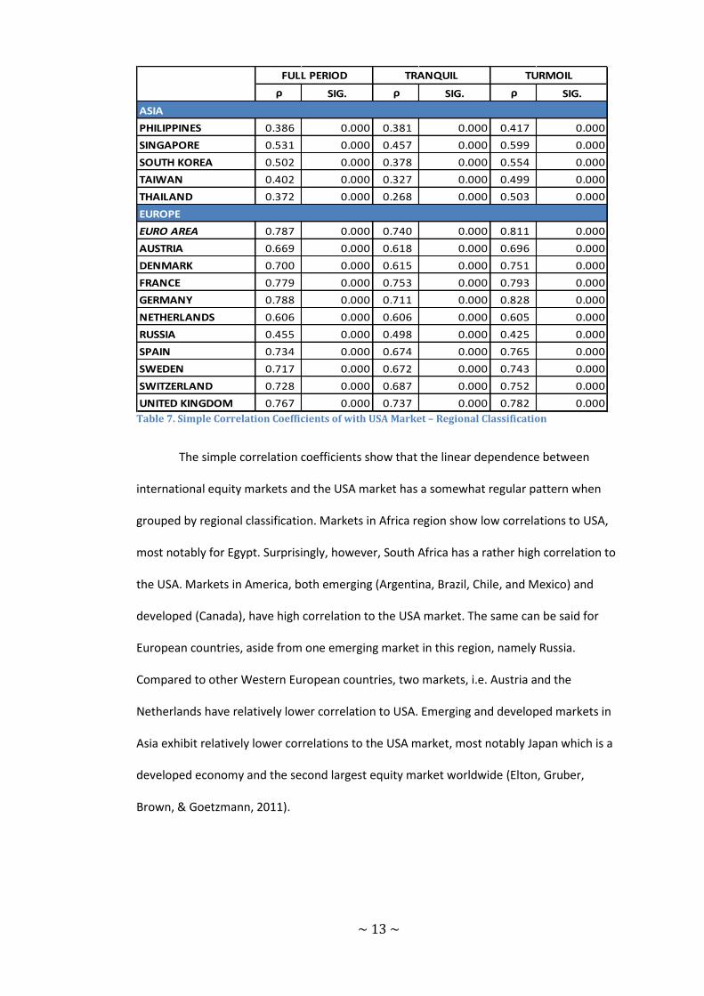
Table 7. Simple Correlation Coefficients of with USA Market – Regional Classification

The simple correlation coefficients show that the linear dependence between

international equity markets and the USA market has a somewhat regular pattern when

grouped by regional classification. Markets in Africa region show low correlations to USA,

most notably for Egypt. Surprisingly, however, South Africa has a rather high correlation to

the USA. Markets in America, both emerging (Argentina, Brazil, Chile, and Mexico) and

developed (Canada), have high correlation to the USA market. The same can be said for

European countries, aside from one emerging market in this region, namely Russia.

Compared to other Western European countries, two markets, i.e. Austria and the

Netherlands have relatively lower correlation to USA. Emerging and developed markets in

Asia exhibit relatively lower correlations to the USA market, most notably Japan which is a

developed economy and the second largest equity market worldwide (Elton, Gruber,

Brown, & Goetzmann, 2011).

~ 14 ~

The estimated coefficients showing non-significant linear dependence to USA are

marked in bold and italic numbers. It is found China has no significant correlation to the

United States during the tranquil and turmoil sub-samples. Even though its correlation to

the United States for the full sample period is significant, albeit very low, China will be

excluded from further analysis. For the rest of the countries considered in this study, all of

the correlation coefficients are statistically significant for α = 5%.

The results suggest that regional proximity play a role on cross-border

interdependence. These findings are in line with those from previous study (Bekaert &

Hodrick, 2009). Re-grouping the countries based on their income-level, the correlations

coefficients are presented as:

~ 15 ~


EGYPT 0.226 0.000 0.172 0.000 0.483 0.031

INDONESIA 0.323 0.000 0.346 0.000 0.305 0.002

INDIA 0.458 0.000 0.355 0.000 0.596 0.000

PHILIPPINES 0.386 0.000 0.381 0.000 0.417 0.000

THAILAND 0.372 0.000 0.268 0.000 0.503 0.000

ARGENTINA 0.695 0.000 0.689 0.000 0.708 0.000

BRAZIL 0.797 0.000 0.785 0.000 0.825 0.000

CHILE 0.704 0.000 0.688 0.000 0.733 0.000

MALAYSIA 0.334 0.000 0.298 0.000 0.439 0.000

MEXICO 0.821 0.000 0.794 0.000 0.843 0.000

RUSSIA 0.455 0.000 0.498 0.000 0.425 0.000

SOUTH AFRICA 0.661 0.000 0.614 0.000 0.702 0.000

AUSTRALIA 0.569 0.000 0.450 0.000 0.652 0.000

AUSTRIA 0.669 0.000 0.618 0.000 0.696 0.000

CANADA 0.828 0.000 0.761 0.000 0.868 0.000

DENMARK 0.700 0.000 0.615 0.000 0.751 0.000

EURO AREA 0.787 0.000 0.740 0.000 0.811 0.000

FRANCE 0.779 0.000 0.753 0.000 0.793 0.000

GERMANY 0.788 0.000 0.711 0.000 0.828 0.000

HONGKONG 0.541 0.000 0.432 0.000 0.625 0.000

ISRAEL 0.507 0.000 0.552 0.000 0.515 0.000

JAPAN 0.426 0.000 0.277 0.000 0.529 0.000

NETHERLANDS 0.606 0.000 0.606 0.000 0.605 0.000

NEW ZEALAND 0.470 0.000 0.364 0.000 0.540 0.000

SINGAPORE 0.531 0.000 0.457 0.000 0.599 0.000

SOUTH KOREA 0.502 0.000 0.378 0.000 0.554 0.000

SPAIN 0.734 0.000 0.674 0.000 0.765 0.000

SWEDEN 0.717 0.000 0.672 0.000 0.743 0.000

SWITZERLAND 0.728 0.000 0.687 0.000 0.752 0.000

UNITED KINGDOM 0.767 0.000 0.737 0.000 0.782 0.000

LOWER-MIDDLE INCOME

UPPER-MIDDLE INCOME

HIGH INCOME


Table 8. Simple Correlation Coefficients with USA Market – Income-Level Classification

From the table above, it can be seen that all of the lower-middle income countries

have low correlation to the USA market. The countries in the upper-middle income group

have high correlation to the United States, except Malaysia and Russia. Most of the

countries in high income group show relatively higher correlation to the USA market

compared to other income groups. The lowest correlation exhibits by a country in this

income level, i.e. possess macroeconomic similarities to the United States, is that

calculated from Japan market

~ 16 ~

As for the coefficients estimated for the two sub-samples, most of these

correlation coefficients show an increase in the crisis sub-sample compared to those in the

tranquil and full periods. This feature of increasing correlations during the crisis-period has

been well documented in previous studies (See, for instance, (King, Sentana, & Wadhwani,

1994; Ramchand & Susmel, 1998; Morana & Beltratti, 2008; Bekaert & Hodrick, 2009). Two

markets show relatively stable correlation coefficients for the three periods, i.e. Israel and

the Netherlands. Two exceptional markets in this study are Russia and Indonesia stock

markets. Their correlations with United States market are lower during the crisis sub-

sample compared to those from either full or tranquil period.

In Russia case, lower correlation coefficient is probably due to the time window

definition for crisis period in this study. The free-fall of stock markets in Russia was

noticeable around mid September and trading in this country was suspended on 17

September 2008 (Bush, 2008). By re-defining the tranquil period from the beginning of data

collection to 31/08/2008 and the crisis period from 01/09/2008 – 31/03/2009, Russia’s

correlations with the USA are 0.401 and 0.466 for the re-defined tranquil and crisis period,

respectively. The result for Indonesian market is an interesting phenomenon, considering

that in October 2008 the trading in Indonesian stock market Jakarta Stock Exchange was

suspended due massive sell-outs (SPIEGEL Staff, 2008). Nevertheless, the heterogeneity of

the direction of cross-market correlation during a high volatility period has been reported

in previous study (Corsetti, Pericoli, & Sbracia, 2001).

~ 17 ~

V.4. SERIAL- AND CROSS-CORRELATION TEST

In order to justify the application of multivariate financial time series, such as

Vector Autoregressive (VAR) model employed in this study, serial- and cross-correlations

between the returns of market j and those of USA are investigated. For covariate m = 2 and

lag order p = 3 the multivariate statistics ( ) are summarized in the table below:

COUNTRY Q2(3) COUNTRY Q2(3) COUNTRY Q2(3)

EGYPT 206.35 AUSTRALIA 604.74 EURO AREA 431.94

ISRAEL 173.80 HONG KONG 373.15 AUSTRIA 450.22

SOUTH AFRICA 407.17 INDONESIA 318.76 DENMARK 417.75

INDIA 261.26 FRANCE 461.73

ARGENTINA 341.92 JAPAN 446.81 GERMANY 356.93

BRAZIL 323.93 MALAYSIA 368.77 NETHERLANDS 646.18

CANADA 325.19 NEW ZEALAND 520.00 RUSSIA 311.73

CHILE 325.09 PHILIPPINES 502.05 SPAIN 426.62

MEXICO 339.91 SINGAPORE 359.00 SWEDEN 402.64

SOUTH KOREA 338.65 SWITZERLAND 383.06

TAIWAN 391.77 UNITED KINGDOM 498.74

THAILAND 306.82

ASIA

AMERICA

EUROPEAFRICA

Table 9. Multivariate Ljung-Box Statistics

The critical value of distribution for α = 5% and degrees of freedom

is 21.026 (Berenson, Levine, & Krehbiel, 2009). Therefore, it can be concluded that all the

returns data in this study have significant serial- and cross-correlations with its past values

and the past values of USA market. Thus, the application of VAR model with p = 3 is

justified to remove these linear dependencies. Since the lag order is found not to change

the conclusion of the conditional correlation analysis (Forbes & Rigobon, 2002), it is not

deemed necessary to perform joint test for longer lag.

V.5. REGRESSION ANALYSIS

For a specified VAR model, the parameters can be estimated using either the

ordinary least squares method (OLS) or the maximum likelihood estimation (Tsay, 2005).

Since the two methods are asymptotically equivalent, the OLS method is chosen for this

~ 18 ~

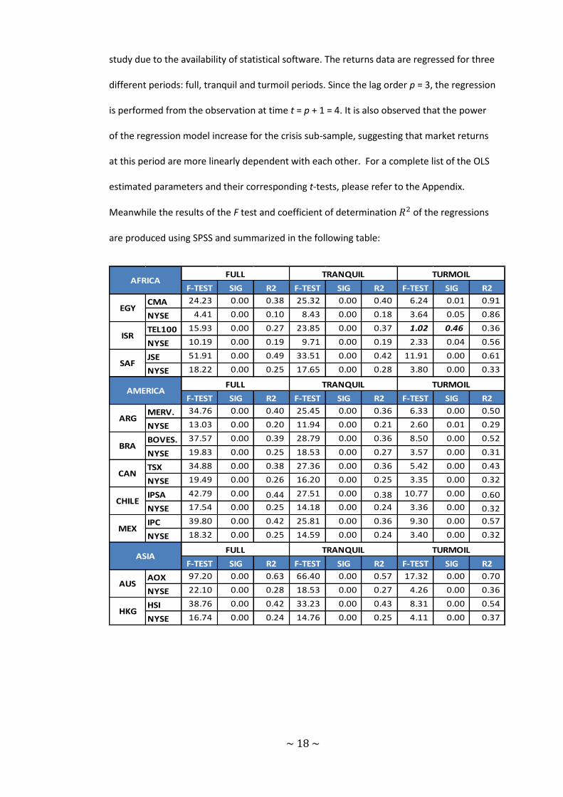
study due to the availability of statistical software. The returns data are regressed for three

different periods: full, tranquil and turmoil periods. Since the lag order p = 3, the regression

is performed from the observation at time t = p + 1 = 4. It is also observed that the power

of the regression model increase for the crisis sub-sample, suggesting that market returns

at this period are more linearly dependent with each other. For a complete list of the OLS

estimated parameters and their corresponding t-tests, please refer to the Appendix.

Meanwhile the results of the F test and coefficient of determination of the regressions

are produced using SPSS and summarized in the following table:

F-TEST SIG R2 F-TEST SIG R2 F-TEST SIG R2

CMA 24.23 0.00 0.38 25.32 0.00 0.40 6.24 0.01 0.91

NYSE 4.41 0.00 0.10 8.43 0.00 0.18 3.64 0.05 0.86

TEL100 15.93 0.00 0.27 23.85 0.00 0.37 1.02 0.46 0.36

NYSE 10.19 0.00 0.19 9.71 0.00 0.19 2.33 0.04 0.56

JSE 51.91 0.00 0.49 33.51 0.00 0.42 11.91 0.00 0.61

NYSE 18.22 0.00 0.25 17.65 0.00 0.28 3.80 0.00 0.33


MERV. 34.76 0.00 0.40 25.45 0.00 0.36 6.33 0.00 0.50

NYSE 13.03 0.00 0.20 11.94 0.00 0.21 2.60 0.01 0.29

BOVES. 37.57 0.00 0.39 28.79 0.00 0.36 8.50 0.00 0.52

NYSE 19.83 0.00 0.25 18.53 0.00 0.27 3.57 0.00 0.31

TSX 34.88 0.00 0.38 27.36 0.00 0.36 5.42 0.00 0.43

NYSE 19.49 0.00 0.26 16.20 0.00 0.25 3.35 0.00 0.32

IPSA 42.79 0.00 0.44 27.51 0.00 0.38 10.77 0.00 0.60

NYSE 17.54 0.00 0.25 14.18 0.00 0.24 3.36 0.00 0.32

IPC 39.80 0.00 0.42 25.81 0.00 0.36 9.30 0.00 0.57

NYSE 18.32 0.00 0.25 14.59 0.00 0.24 3.40 0.00 0.32


AOX 97.20 0.00 0.63 66.40 0.00 0.57 17.32 0.00 0.70

NYSE 22.10 0.00 0.28 18.53 0.00 0.27 4.26 0.00 0.36

HSI 38.76 0.00 0.42 33.23 0.00 0.43 8.31 0.00 0.54

NYSE 16.74 0.00 0.24 14.76 0.00 0.25 4.11 0.00 0.37

TRANQUIL TURMOIL

AUS

HKG

ASIA

EGY

AFRICA

AMERICA

FULL

TRANQUIL TURMOIL

FULL TRANQUIL TURMOIL

MEX

ISR

SAF

FULL

ARG

BRA

CAN

CHILE

~ 19 ~


JKSE 33.89 0.00 0.40 29.04 0.00 0.39 5.07 0.00 0.46

NYSE 15.26 0.00 0.23 16.31 0.00 0.27 2.08 0.03 0.26

BSE30 25.94 0.00 0.34 28.81 0.00 0.39 4.06 0.00 0.42

NYSE 14.32 0.00 0.22 12.81 0.00 0.22 2.12 0.03 0.27

NIKKEI 61.08 0.00 0.54 31.17 0.00 0.41 14.79 0.00 0.71

NYSE 12.79 0.00 0.20 12.05 0.00 0.21 2.86 0.00 0.32

KLCI 39.40 0.00 0.43 44.36 0.00 0.50 4.86 0.00 0.45

NYSE 15.37 0.00 0.23 14.61 0.00 0.24 2.85 0.00 0.32

NZX50 73.41 0.00 0.57 52.84 0.00 0.53 14.22 0.00 0.66

NYSE 18.48 0.00 0.25 18.88 0.00 0.28 3.42 0.00 0.32

PSEI20 74.68 0.00 0.59 53.30 0.00 0.55 23.69 0.00 0.77

NYSE 21.86 0.00 0.29 16.74 0.00 0.27 4.57 0.00 0.39

STI 32.83 0.00 0.37 35.05 0.00 0.43 4.75 0.00 0.40

NYSE 18.32 0.00 0.25 17.54 0.00 0.27 3.77 0.00 0.35

KOSPI 39.67 0.00 0.43 28.19 0.00 0.39 7.13 0.00 0.50

NYSE 18.28 0.00 0.26 9.31 0.00 0.17 4.53 0.00 0.38

TWSE 42.19 0.00 0.44 34.93 0.00 0.44 8.65 0.00 0.56

NYSE 19.17 0.00 0.27 16.95 0.00 0.27 3.03 0.00 0.31

S.E.T 28.23 0.00 0.36 18.23 0.00 0.30 8.17 0.00 0.27

NYSE 14.49 0.00 0.22 11.97 0.00 0.22 3.23 0.00 0.32


STOXX50 58.70 0.00 0.50 33.55 0.00 0.40 11.23 0.00 0.59

NYSE 20.19 0.00 0.26 18.02 0.00 0.27 4.13 0.00 0.35

ATX 56.70 0.00 0.51 31.65 0.00 0.41 11.94 0.00 0.62

NYSE 17.10 0.00 0.24 14.09 0.00 0.24 3.73 0.00 0.34

OMXC 65.42 0.00 0.54 37.37 0.00 0.44 13.09 0.00 0.63

NYSE 19.99 0.00 0.26 17.84 0.00 0.27 3.88 0.00 0.34

CAC40 61.44 0.00 0.51 34.17 0.00 0.41 12.09 0.00 0.61

NYSE 20.20 0.00 0.26 18.13 0.00 0.27 4.12 0.00 0.35

DAX30 48.94 0.00 0.46 32.50 0.00 0.40 8.23 0.00 0.52

NYSE 20.94 0.00 0.26 18.46 0.00 0.27 4.13 0.00 0.35

AEX 34.70 0.00 0.37 18.30 0.00 0.27 9.26 0.00 0.55

NYSE 87.08 0.00 0.60 56.61 0.00 0.53 17.37 0.00 0.69

RTSI 33.51 0.00 0.39 31.37 0.00 0.41 5.75 0.00 0.47

NYSE 18.42 0.00 0.26 15.46 0.00 0.26 3.58 0.00 0.36

MSE 59.94 0.00 0.51 31.69 0.00 0.39 11.80 0.00 0.61

NYSE 20.46 0.00 0.26 17.34 0.00 0.26 4.12 0.00 0.35

OMXS 56.40 0.00 0.50 35.67 0.00 0.43 10.17 0.00 0.58

NYSE 18.97 0.00 0.25 15.94 0.00 0.25 3.68 0.00 0.33

SSMI 57.40 0.00 0.50 28.08 0.00 0.37 14.39 0.00 0.65

NYSE 18.43 0.00 0.25 14.84 0.00 0.24 4.41 0.00 0.37

FTSE100 5.13 0.00 0.42 38.50 0.00 0.44 10.47 0.00 0.57

NYSE 7.01 0.00 0.50 19.14 0.00 0.28 3.78 0.00 0.33

SWE

SWI

UK

DEN

FRA

GER

NED

RUS

SPA


EUR

EUROPE

AUT

PHI

SIG

S.KOR

TAI

THA

NZ

INA

IND

JAP

MAL

ASIAFULL TRANQUIL TURMOIL

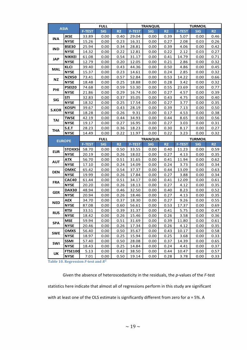
Table 10. Regression F-test and

Given the absence of heteroscedasticity in the residuals, the p-values of the F-test

statistics here indicate that almost all of regressions perform in this study are significant

with at least one of the OLS estimate is significantly different from zero for α = 5%. A

~ 20 ~

regression for Israel market for the crisis sub-sample found to be insignificant, i.e. all of its

parameters are not significantly different from zero. Therefore we exclude Israel from

further analysis.

The of the regression signifies the explanatory power of the fitted model

(Berenson, Levine, & Krehbiel, 2009). From the regression s of the VAR(3) model in this

study it can be conjectured that in general, USA market is less dependent on serial- and

cross-correlation with market j as indicated by the lower for regression perform on USA

market returns. Exceptions are Thailand in crisis period, the Netherlands for all periods, and

United Kingdom for full period. When for USA market is found to be larger than those

for the market j, it indicates that the latter is less dependent of serial- and cross-correlation

with USA. Nevertheless, by looking at individual t-test of the regression parameter, it can

be concluded that, holding other explanatory variables constant, most of the equity

markets exhibits pronounced cross-correlation with past values of USA market, except for

Egypt.

In addition to lower for the regression of USA return, the exogeneity of this

market is evidence on the p-values of t-test for each of its estimated parameters for lagged

returns of market j. Almost all past values of market j have no significant impact on USA

return. Only in tranquil period regression on Hong Kong past values there appears to be

some feedback to USA. The results of regression suggest that USA market is less dependent

on the feedback from other markets. Therefore it can be concluded that the exogeneity

assumption of the USA market is a reasonable one. The granger causality of USA market,

especially on Asian markets, has been suggested by previous study (Atteberry & Swanson,

1997; Cha & Cheung., 1998; Cheung, Cheung, & Ng, 2007; Ding, 2010).

~ 21 ~

The t-test of the constant term show that almost all of the intercepts are not

significantly different from zero. The p-values also suggest that serial correlation of market

j appears to become less significant during crisis period. The same pattern is also observed

for USA market, its linear dependence on its past values appear to decline during turmoil

times. Exceptions to this are observed in countries in Europe region. Most countries in this

region show pronounced serial correlation in all periods. United Kingdom becomes more

serially correlated in crisis period. From all European countries, only Russia shows a

decrease in serial correlation during high volatility period. Taking the joint impact of all the

explanatory variables into consideration, the linear dependence between market j and USA

market appears to increase during the turmoil period as indicated by the increase in

values for this period.

Regarding past values of interest rates, the dependence of each of market returns

on their respective interest rates and of USA interest rates is less significant. However, it is

observed that there is a dependence of USA return is on daily short-term interest rates of

several markets, namely Japan and United Kingdom.

V.6. RESIDUALS ANALYSIS

In order to proceed with the correlation analysis, the regression residuals are

analysed to test whether assumptions underlying the OLS estimation are not violated.

Residuals analysis is also necessary to determine whether the fitted model selected is an

appropriate model. There are four assumptions of regression, namely: linearity,

independence of errors, normality of error and equal variance (Berenson, Levine, &

Krehbiel, 2009). As mentioned previously, the normality of the residuals is not analysed

because of large sample justification.

~ 22 ~

Linearity testing of residuals is a procedure to check whether there is a relationship

between the explanatory variables and the residuals. The residuals series are found to

be uncorrelated with the past value (p > 0) for all time series models (Tsay, 2005). Due

to the time constraint, any relationship between residuals and the past values of interest

rates will be assumed away. The robustness of this assumption will be tested in the

sensitivity analysis by removing the lagged values of interest rates from the right hand side

(RHS) variables and compare the resulting correlation to that of the original model which

include lagged interest rates as RHS variables.

Therefore we proceed with the Durbin-Watson (DW) test to check the serial

correlation of the residuals. The DW statistics are produced using SPSS and the results are

as follows:

AFRICA MKT. J MKT. USA MKT. J MKT. USA MKT. J MKT. USA

EGYPT 1.99 1.98 2.00 2.00 2.42 1.86

ISRAEL 1.96 2.00 1.93 1.98 2.01 2.11

SOUTH AFRICA 1.97 1.97 1.94 1.97 1.91 2.00

AMERICA MKT. J MKT. USA MKT. J MKT. USA MKT. J MKT. USA

ARGENTINA 1.94 1.99 1.97 1.97 1.87 2.03

BRAZIL 1.96 1.97 1.92 1.94 2.02 2.00

CANADA 1.89 1.94 1.87 1.93 1.88 1.93

CHILE 1.98 1.98 1.95 1.94 2.03 2.05

MEXICO 1.99 1.98 1.98 1.96 1.97 2.00

ASIA MKT. J MKT. USA MKT. J MKT. USA MKT. J MKT. USA

AUSTRALIA 1.99 1.96 1.96 1.94 1.96 1.95

HONG KONG 1.94 1.92 1.97 1.97 1.91 1.90

INDONESIA 2.02 2.02 1.99 1.89 2.00 2.10

INDIA 1.96 1.90 1.98 1.97 1.89 1.78

JAPAN 1.96 1.98 1.95 1.99 1.95 1.95

MALAYSIA 1.95 2.01 1.88 1.99 2.03 2.03

NEW ZEALAND 2.00 2.00 1.95 1.95 1.97 2.04

PHILIPPINES 1.91 1.96 1.91 2.00 1.83 1.92

SINGAPORE 2.00 2.00 1.97 1.97 1.99 2.07

SOUTH KOREA 1.99 1.94 1.99 1.94 1.99 1.93

TAIWAN 1.98 1.94 1.98 1.95 1.93 1.97

THAILAND 1.96 2.01 1.92 1.96 1.96 1.96


~ 23 ~

EUROPE MKT. J MKT. USA MKT. J MKT. USA MKT. J MKT. USA

EURO AREA 1.87 1.91 1.89 1.94 1.75 1.90

AUSTRIA 1.93 1.98 1.93 1.96 1.81 1.97

DENMARK 1.84 1.94 1.91 1.95 1.68 1.95

FRANCE 1.85 1.91 1.88 1.94 1.72 1.91

GERMANY 1.89 1.93 1.92 1.95 1.83 1.93

NETHERLANDS 1.96 1.95 1.98 1.97 1.90 2.00

RUSSIA 2.01 1.96 1.92 1.91 2.06 2.00

SPAIN 1.87 1.93 1.91 1.98 1.72 1.72

SWEDEN 1.87 1.93 1.92 1.95 1.71 1.92

SWITZERLAND 1.87 1.95 1.90 1.96 1.74 1.99

UNITED KINGDOM 1.93 1.93 1.96 1.95 1.72 1.92


Table 11. Durbin-Watson Statistics of Regression Residuals

From the DW-statistics of market returns for all periods considered, it can be seen

that all values of DW statistics are close to 2. Therefore, it can be safely concluded that the

residuals obtained from this regression model are not serially correlated (Berenson, Levine,

& Krehbiel, 2009).

The Levene tests are performed on both the Australia market and the USA market

for full period. The residuals from each market are divided into ten sub-groups. The median

is selected for the equal variance test because it is has been suggested that employing

median instead of mean for Levene test provides good robustness against many types of

non-normal data while simultaneously maintaining good test power (NIST/SEMATECH).

The test statistics are LW = 1.15 and 0.56 for Australia and USA market,

respectively. The critical value of distribution with degree of freedom 699 for numerator

and 9 for denominator at level of significance α = 5% is 2.71 (Berenson, Levine, & Krehbiel,

2009). Therefore we do not reject the null hypothesis of equal variance. This statistic is

produced using Excel due to the non-availability of other statistical software. With limited

time available at hand, the possibilities of violation to residuals homoscedasticity

assumption for other markets are assumed away.

~ 24 ~

V.7. CORRELATION ANALYSIS

V.7.1. CONDITIONAL CORRELATION COEFFICIENTS

By conditioning the returns matrix on the past values of market j and USA market

and the past values of interest rates from each market, the linear dependence between

market j and USA market for each period and their significance tests are summarized in the

following table:

TRANQUIL SIG. CRISIS SIG.

EGYPT 0.175 0.000 0.149 0.001 0.178 0.452

SOUTH AFRICA 0.620 0.000 0.548 0.000 0.707 0.000

ARGENTINA 0.709 0.000 0.709 0.000 0.728 0.000

BRAZIL 0.786 0.000 0.778 0.000 0.831 0.000

CANADA 0.827 0.000 0.761 0.000 0.880 0.000

CHILE 0.702 0.000 0.687 0.000 0.748 0.000

MEXICO 0.825 0.000 0.794 0.000 0.884 0.000

AUSTRALIA 0.516 0.000 0.364 0.000 0.655 0.000

HONGKONG 0.496 0.000 0.350 0.000 0.625 0.000

INDONESIA 0.274 0.000 0.305 0.000 0.273 0.012

INDIA 0.465 0.000 0.305 0.000 0.662 0.000

JAPAN 0.289 0.000 0.158 0.000 0.395 0.000

MALAYSIA 0.290 0.000 0.240 0.000 0.416 0.000

NEW ZEALAND 0.402 0.000 0.257 0.000 0.501 0.000

PHILIPPINES 0.250 0.000 0.278 0.000 0.281 0.005

SINGAPORE 0.476 0.000 0.367 0.000 0.549 0.000

SOUTH KOREA 0.422 0.000 0.279 0.000 0.477 0.000

TAIWAN 0.291 0.000 0.216 0.000 0.410 0.000

THAILAND 0.335 0.000 0.204 0.000 0.486 0.000

ASIA

FULL VAR SIG. SEPARATE VAR

AFRICA

AMERICA

~ 25 ~


EURO AREA 0.764 0.000 0.721 0.000 0.797 0.000

AUSTRIA 0.653 0.000 0.609 0.000 0.673 0.000

DENMARK 0.665 0.000 0.589 0.000 0.741 0.000

FRANCE 0.755 0.000 0.733 0.000 0.774 0.000

GERMANY 0.751 0.000 0.688 0.000 0.792 0.000

NETHERLANDS 0.462 0.000 0.474 0.000 0.386 0.000

RUSSIA 0.414 0.000 0.461 0.000 0.377 0.000

SPAIN 0.710 0.000 0.659 0.000 0.760 0.000

SWEDEN 0.682 0.000 0.656 0.000 0.704 0.000

SWITZERLAND 0.688 0.000 0.666 0.000 0.706 0.000

UNITED KINGDOM 0.754 0.000 0.719 0.000 0.787 0.000

EUROPE


Table 12. Conditional Correlation Coefficients by Regional Classification

All of the conditional correlations in Table 13 are statistically significant, except for

the correlation coefficient between Egypt and USA during the crisis period (marked in bold

and italic number). Therefore, Egypt will be excluded from further analysis.

Given the past values of the common factors, the conditional correlations between

market j and USA market show the same tendency as that of the simple coefficients.

Markets in America and Europe regions show high correlations with USA market, except for

the Netherlands and Russia. Both emerging and developed markets in Asia region show

relatively lower conditional correlation to the market in the United States. The results for

Africa region show a fragmented view. A less developed market such as Egypt show a very

low correlation to USA, with its coefficient during the high volatility period is not

statistically different from zero. On the other hand, a more developed market like South

Africa shows high correlation to USA.

By removing any serial- and cross-correlation in the market returns, the calculated

conditional correlation coefficients are in general lower than the simple coefficients in

Table 8 except for several countries. Those that are found to exhibit higher conditional

~ 26 ~

correlations are countries in America region. For countries in this region, the calculation

results show that the conditional correlation is relatively the same or higher than the

simple coefficient.

Grouping the countries based on their income-level, the conditional correlation

coefficients can be presented as:


EGYPT 0.175 0.000 0.149 0.001 0.178 0.452

INDONESIA 0.274 0.000 0.305 0.000 0.273 0.012

INDIA 0.465 0.000 0.305 0.000 0.662 0.000

PHILIPPINES 0.250 0.000 0.278 0.000 0.281 0.005

THAILAND 0.335 0.000 0.204 0.000 0.486 0.000

ARGENTINA 0.709 0.000 0.709 0.000 0.728 0.000

BRAZIL 0.786 0.000 0.778 0.000 0.831 0.000

CHILE 0.702 0.000 0.687 0.000 0.748 0.000

MALAYSIA 0.290 0.000 0.240 0.000 0.416 0.000

MEXICO 0.825 0.000 0.794 0.000 0.884 0.000

RUSSIA 0.414 0.000 0.461 0.000 0.377 0.000

SOUTH AFRICA 0.620 0.000 0.548 0.000 0.707 0.000

AUSTRALIA 0.516 0.000 0.364 0.000 0.655 0.000

AUSTRIA 0.653 0.000 0.609 0.000 0.673 0.000

CANADA 0.827 0.000 0.761 0.000 0.880 0.000

DENMARK 0.665 0.000 0.589 0.000 0.741 0.000

EURO AREA 0.764 0.000 0.721 0.000 0.797 0.000

FRANCE 0.755 0.000 0.733 0.000 0.774 0.000

GERMANY 0.751 0.000 0.688 0.000 0.792 0.000

HONGKONG 0.496 0.000 0.350 0.000 0.625 0.000

JAPAN 0.289 0.000 0.158 0.000 0.395 0.000

HIGH INCOME


LOWER-MIDDLE INCOME

UPPER-MIDDLE INCOME

~ 27 ~


NETHERLANDS 0.462 0.000 0.474 0.000 0.386 0.000

NEW ZEALAND 0.402 0.000 0.257 0.000 0.501 0.000

SINGAPORE 0.476 0.000 0.367 0.000 0.549 0.000

SOUTH KOREA 0.422 0.000 0.279 0.000 0.477 0.000

SPAIN 0.710 0.000 0.659 0.000 0.760 0.000

SWEDEN 0.682 0.000 0.656 0.000 0.704 0.000

SWITZERLAND 0.688 0.000 0.666 0.000 0.706 0.000

UNITED KINGDOM 0.754 0.000 0.719 0.000 0.787 0.000


HIGH INCOME

Table 13. Conditional Correlation Coefficients by Income Level Classification

The same conclusion can be discerned as that obtained from the calculation of

simple correlation coefficient. All of the lower-middle income countries have low

conditional correlation to the USA market. The countries in the upper-middle income group

have high correlation to the United States, except Malaysia and Russia. Most of the high

income countries show relatively high correlation to the USA market, notably those in the

Europe region. High income countries with relatively lower correlations are those in Asia

region and the Netherlands. Japan shows the lowest correlation for this group of income-

level.

On the other hand, almost all conditional correlations are higher during the crisis

period compared to those in the full and tranquil period, save for Indonesia, the

Netherlands and Russia. However, as stated by Forbes and Rigobon (2001; 2002), this

relatively higher correlation during the crisis period does not translate into contagion if the

increase between the turmoil times relative to the low volatility period is not statistically

significant. Following their methodology, conditional correlation coefficient for the crisis

period is estimated from the full period OLS residuals for each economy. These coefficients

for full and crisis periods are then adjusted for heteroscedasticity effect by taking into

account the relative increase of variance of returns in the crisis country.

~ 28 ~

The relative increase of variance is calculated between the two different periods:

turmoil and relatively low volatility periods. Following Forbes and Rigobon method, it is

calculated between crisis and full sample period. The USA market variance during crisis is

around 3.5 times higher compared to that in a more tranquil period.

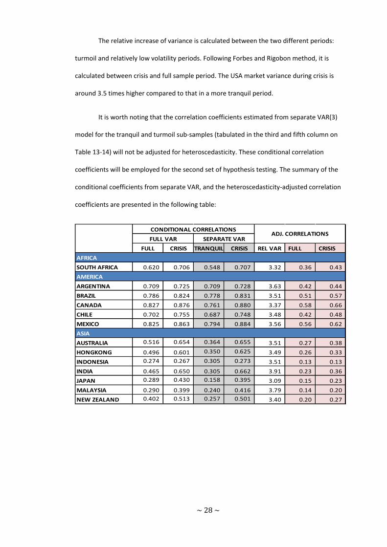
It is worth noting that the correlation coefficients estimated from separate VAR(3)

model for the tranquil and turmoil sub-samples (tabulated in the third and fifth column on

Table 13-14) will not be adjusted for heteroscedasticity. These conditional correlation

coefficients will be employed for the second set of hypothesis testing. The summary of the

conditional coefficients from separate VAR, and the heteroscedasticity-adjusted correlation

coefficients are presented in the following table:

FULL CRISIS TRANQUIL CRISIS REL VAR FULL CRISIS

SOUTH AFRICA 0.620 0.706 0.548 0.707 3.32 0.36 0.43

ARGENTINA 0.709 0.725 0.709 0.728 3.63 0.42 0.44

BRAZIL 0.786 0.824 0.778 0.831 3.51 0.51 0.57

CANADA 0.827 0.876 0.761 0.880 3.37 0.58 0.66

CHILE 0.702 0.755 0.687 0.748 3.48 0.42 0.48

MEXICO 0.825 0.863 0.794 0.884 3.56 0.56 0.62

AUSTRALIA 0.516 0.654 0.364 0.655 3.51 0.27 0.38

HONGKONG 0.496 0.601 0.350 0.625 3.49 0.26 0.33

INDONESIA 0.274 0.267 0.305 0.273 3.51 0.13 0.13

INDIA 0.465 0.650 0.305 0.662 3.91 0.23 0.36

JAPAN 0.289 0.430 0.158 0.395 3.09 0.15 0.23

MALAYSIA 0.290 0.399 0.240 0.416 3.79 0.14 0.20

NEW ZEALAND 0.402 0.513 0.257 0.501 3.40 0.20 0.27

AMERICA

ASIA

CONDITIONAL CORRELATIONSADJ. CORRELATIONS

FULL VAR SEPARATE VAR

AFRICA

~ 29 ~

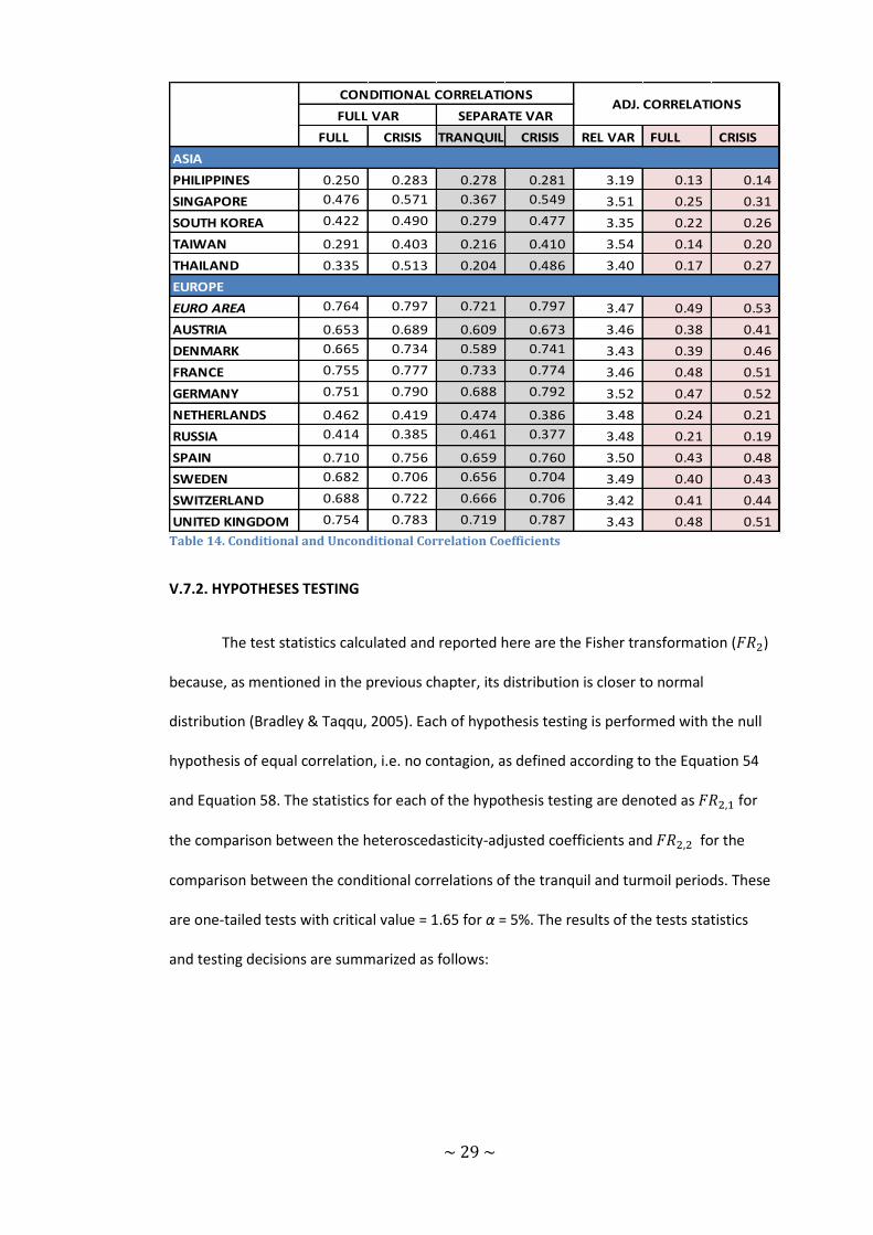
FULL CRISIS TRANQUIL CRISIS REL VAR FULL CRISIS

PHILIPPINES 0.250 0.283 0.278 0.281 3.19 0.13 0.14

SINGAPORE 0.476 0.571 0.367 0.549 3.51 0.25 0.31

SOUTH KOREA 0.422 0.490 0.279 0.477 3.35 0.22 0.26

TAIWAN 0.291 0.403 0.216 0.410 3.54 0.14 0.20

THAILAND 0.335 0.513 0.204 0.486 3.40 0.17 0.27

EURO AREA 0.764 0.797 0.721 0.797 3.47 0.49 0.53

AUSTRIA 0.653 0.689 0.609 0.673 3.46 0.38 0.41

DENMARK 0.665 0.734 0.589 0.741 3.43 0.39 0.46

FRANCE 0.755 0.777 0.733 0.774 3.46 0.48 0.51

GERMANY 0.751 0.790 0.688 0.792 3.52 0.47 0.52

NETHERLANDS 0.462 0.419 0.474 0.386 3.48 0.24 0.21

RUSSIA 0.414 0.385 0.461 0.377 3.48 0.21 0.19

SPAIN 0.710 0.756 0.659 0.760 3.50 0.43 0.48

SWEDEN 0.682 0.706 0.656 0.704 3.49 0.40 0.43

SWITZERLAND 0.688 0.722 0.666 0.706 3.42 0.41 0.44

UNITED KINGDOM 0.754 0.783 0.719 0.787 3.43 0.48 0.51

EUROPE

ASIA

CONDITIONAL CORRELATIONSADJ. CORRELATIONS

FULL VAR SEPARATE VAR

Table 14. Conditional and Unconditional Correlation Coefficients

V.7.2. HYPOTHESES TESTING

The test statistics calculated and reported here are the Fisher transformation ( )

because, as mentioned in the previous chapter, its distribution is closer to normal

distribution (Bradley & Taqqu, 2005). Each of hypothesis testing is performed with the null

hypothesis of equal correlation, i.e. no contagion, as defined according to the Equation 54

and Equation 58. The statistics for each of the hypothesis testing are denoted as for

the comparison between the heteroscedasticity-adjusted coefficients and for the

comparison between the conditional correlations of the tranquil and turmoil periods. These

are one-tailed tests with critical value = 1.65 for α = 5%. The results of the tests statistics

and testing decisions are summarized as follows:

~ 30 ~

FULL TRA CRI SE FR2,1 CONT. SE FR2,2 CONT.

SOUTH AFRICA 672 568 104 0.11 0.86 NO 0.11 2.46 YES

ARGENTINA 644 554 90 0.11 0.17 NO 0.12 0.34 NO

BRAZIL 730 623 107 0.10 0.70 NO 0.11 1.43 NO

CANADA 695 595 100 0.11 1.19 NO 0.11 3.44 YES

CHILE 659 559 100 0.11 0.65 NO 0.11 1.15 NO

MEXICO 666 568 98 0.11 0.84 NO 0.11 2.81 YES

AUSTRALIA 709 605 104 0.11 1.09 NO 0.11 3.74 YES

HONGKONG 648 551 97 0.11 0.74 NO 0.11 3.29 YES

INDONESIA 631 547 84 0.12 0.03- NO 0.12 0.29- NO

INDIA 629 548 81 0.12 1.19 NO 0.12 3.98 YES

JAPAN 629 543 86 0.12 0.72 NO 0.12 2.19 YES

MALAYSIA 643 558 85 0.12 0.51 NO 0.12 1.67 YES

NEW ZEALAND 685 585 100 0.11 0.68 NO 0.11 2.62 YES

PHILIPPINES 646 546 100 0.11 0.17 NO 0.11 0.03 NO

SINGAPORE 675 578 97 0.11 0.63 NO 0.11 2.09 YES

SOUTH KOREA 641 541 100 0.11 0.41 NO 0.11 2.11 YES

TAIWAN 647 552 95 0.11 0.56 NO 0.11 1.92 YES

THAILAND 621 526 95 0.11 1.01 NO 0.11 2.87 YES

EURO AREA 714 608 106 0.11 0.52 NO 0.11 1.69 YES

AUSTRIA 659 560 99 0.11 0.35 NO 0.11 0.99 NO

DENMARK 690 586 104 0.11 0.77 NO 0.11 2.57 YES

FRANCE 715 609 106 0.11 0.33 NO 0.11 0.89 NO

GERMANY 711 607 104 0.11 0.58 NO 0.11 2.16 YES

NETHERLANDS 712 607 105 0.11 0.26- NO 0.11 1.01- NO

RUSSIA 644 553 91 0.11 0.15- NO 0.11 0.89- NO

SPAIN 708 604 104 0.11 0.58 NO 0.11 1.91 YES

SWEDEN 686 584 102 0.11 0.25 NO 0.11 0.82 NO

SWITZERLAND 690 586 104 0.11 0.39 NO 0.11 0.70 NO

UNITED KINGDOM 708 602 106 0.11 0.44 NO 0.11 1.48 NO

EUROPE

SAMPLE SIZE FISHER TRANS.1 FISHER TRANS.2

AFRICA

AMERICA

ASIA

Table 15. Fisher Transformation Statistics by Regional Classification

The results of the first hypothesis testing are in agreement with those found by

Forbes and Rigobon. Virtually there was no shift-contagion found in the stock market crash

of 2008. The test statistics calculated for the unconditional correlation for all countries

suggested that widespread shift-contagion did not occur during the stock market crash of

2008 and there was only a continuance of, albeit high, comovement between the United

~ 31 ~

States and other markets. The results from the first hypothesis testing appear to support

the non-crisis-contingent theory, i.e. there is no change in the propagation mechanisms.

However, the tests performed using conditional correlation coefficients from

separate VARs present different results. As suggested by Dungey and Zhumabekova (2001),

a more powerful test is to perform separate estimation of the VAR model for tranquil and

turmoil periods and compare the resulting conditional correlation coefficients between the

two periods. Following this procedure, it is found that several countries experienced shift-

contagion during the period investigated in this study. In other words, there was a

significant increase of correlation coefficient observed in the crisis period compared to that

in a relatively low volatility period.

In Africa region, South Africa is found to be highly correlated with USA market.

During the crisis period defined in this study, there is evidence of shift-contagion in this

market. In America region, only Canada and Mexico are found to exhibit shift-contagion

during the turmoil period. There is evidence of significant increase in market linkages

between USA and each of the market in Asia region, whether developed (e.g. Japan) or

emerging ones, except for Indonesia and the Philippines. On the other hand, most of the

markets in Europe did not experience shift-contagion except for the aggregate market of

Euro Area, Denmark, Germany, and Spain.

Relying on the second hypothesis testing and grouping the countries into their

income-level, the data presents a clearer pattern:

~ 32 ~

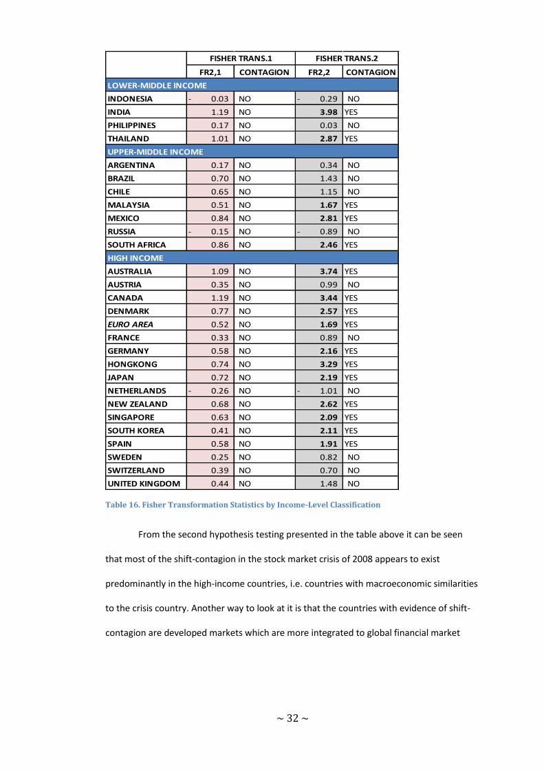
FR2,1 CONTAGION FR2,2 CONTAGION

INDONESIA 0.03- NO 0.29- NO

INDIA 1.19 NO 3.98 YES

PHILIPPINES 0.17 NO 0.03 NO

THAILAND 1.01 NO 2.87 YES

ARGENTINA 0.17 NO 0.34 NO

BRAZIL 0.70 NO 1.43 NO

CHILE 0.65 NO 1.15 NO

MALAYSIA 0.51 NO 1.67 YES

MEXICO 0.84 NO 2.81 YES

RUSSIA 0.15- NO 0.89- NO

SOUTH AFRICA 0.86 NO 2.46 YES

AUSTRALIA 1.09 NO 3.74 YES

AUSTRIA 0.35 NO 0.99 NO

CANADA 1.19 NO 3.44 YES

DENMARK 0.77 NO 2.57 YES

EURO AREA 0.52 NO 1.69 YES

FRANCE 0.33 NO 0.89 NO

GERMANY 0.58 NO 2.16 YES

HONGKONG 0.74 NO 3.29 YES

JAPAN 0.72 NO 2.19 YES

NETHERLANDS 0.26- NO 1.01- NO

NEW ZEALAND 0.68 NO 2.62 YES

SINGAPORE 0.63 NO 2.09 YES

SOUTH KOREA 0.41 NO 2.11 YES

SPAIN 0.58 NO 1.91 YES

SWEDEN 0.25 NO 0.82 NO

SWITZERLAND 0.39 NO 0.70 NO

UNITED KINGDOM 0.44 NO 1.48 NO

FISHER TRANS.1 FISHER TRANS.2

LOWER-MIDDLE INCOME

UPPER-MIDDLE INCOME

HIGH INCOME

Table 16. Fisher Transformation Statistics by Income-Level Classification

From the second hypothesis testing presented in the table above it can be seen

that most of the shift-contagion in the stock market crisis of 2008 appears to exist

predominantly in the high-income countries, i.e. countries with macroeconomic similarities

to the crisis country. Another way to look at it is that the countries with evidence of shift-

contagion are developed markets which are more integrated to global financial market

~ 33 ~

where the United States is the most dominant player. Therefore, they are more at risk to

shock propagated from USA.

Looking at the correlation coefficients between market j and USA, there appear to

be a relationship between high market interdependence and their regional proximity.

However, the results from correlation test do not suggest a pronounced linkage between

regional proximity to the crisis country and shift-contagion. Relying on the results

calculated from the conditional correlation coefficient, shift-contagion appears to be more

pronounced in the Asia region, most notably those with high income level.

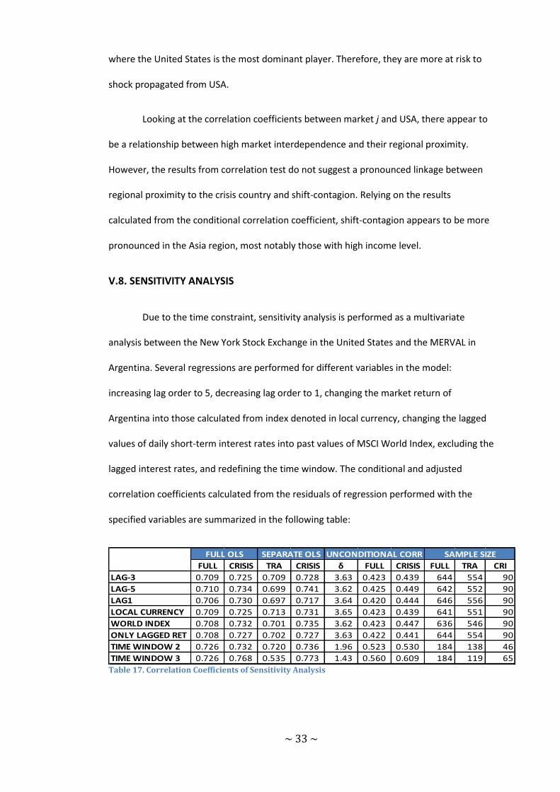
V.8. SENSITIVITY ANALYSIS

Due to the time constraint, sensitivity analysis is performed as a multivariate

analysis between the New York Stock Exchange in the United States and the MERVAL in

Argentina. Several regressions are performed for different variables in the model:

increasing lag order to 5, decreasing lag order to 1, changing the market return of

Argentina into those calculated from index denoted in local currency, changing the lagged

values of daily short-term interest rates into past values of MSCI World Index, excluding the

lagged interest rates, and redefining the time window. The conditional and adjusted

correlation coefficients calculated from the residuals of regression performed with the

specified variables are summarized in the following table:

FULL CRISIS TRA CRISIS δ FULL CRISIS FULL TRA CRI

LAG-3 0.709 0.725 0.709 0.728 3.63 0.423 0.439 644 554 90

LAG-5 0.710 0.734 0.699 0.741 3.62 0.425 0.449 642 552 90

LAG1 0.706 0.730 0.697 0.717 3.64 0.420 0.444 646 556 90

LOCAL CURRENCY 0.709 0.725 0.713 0.731 3.65 0.423 0.439 641 551 90

WORLD INDEX 0.708 0.732 0.701 0.735 3.62 0.423 0.447 636 546 90

ONLY LAGGED RET 0.708 0.727 0.702 0.727 3.63 0.422 0.441 644 554 90

TIME WINDOW 2 0.726 0.732 0.720 0.736 1.96 0.523 0.530 184 138 46

TIME WINDOW 3 0.726 0.768 0.535 0.773 1.43 0.560 0.609 184 119 65

FULL OLS SEPARATE OLS UNCONDITIONAL CORR SAMPLE SIZE

Table 17. Correlation Coefficients of Sensitivity Analysis

~ 34 ~

The test statistics for the differences between correlation coefficient of the crisis

and of the relatively low volatility period are:

SE FR2,1 CONTAGION SE FR2,2 CONTAGION

LAG-3 0.11 0.17 NO 0.12 0.34 NO

LAG-5 0.11 0.26 NO 0.12 0.76 NO

LAG1 0.11 0.26 NO 0.12 0.35 NO

LOCAL CURRENCY 0.11 0.17 NO 0.12 0.32 NO

WORLD INDEX 0.11 0.26 NO 0.12 0.61 NO

ONLY LAGGED RET 0.11 0.20 NO 0.12 0.44 NO

TIME WINDOW 2 0.17 0.06 NO 0.18 0.19 NO

TIME WINDOW 3 0.15 0.51 NO 0.16 2.74 YES

FISHER TRANS. 2FISHER TRANS.1

Table 18. Fisher Transformation Statistics of Sensitivity Analysis

The results of the sensitivity analysis show that both hypothesis testing methods

are quite robust toward lag order. No different results obtained for different lag order, i.e.

no shift-contagion is found for Argentina stock market in the time period considered.

Changing the currency into local currency also does not affect the conclusion for this

market. Sensitivity analysis are also carried out by changing the common factor into past

values of a global index, in this study the global index chosen is MSCI World Index, and by

excluding aggregate shocks altogether. Changing the variables of the common factors does

not affect the results of the correlation rest. No shift-contagion is found in Argentina during

the stock market crash of 2008.

Some suggested that Forbes and Rigobon correlation analysis method consistently

over-rejects the hypothesis of contagion mostly due to the comparison of large sample of

non-crisis period to a small sample of crisis period (Dungey & Zhumabekova, 2001).

Therefore the analysis of time window sensitivity will be performed with different length of

crisis period. By shortening the length of both tranquil and turmoil period, i.e. changing

sample sizes, we come to the same conclusion as that obtained with longer period.

However, changing the specification of the turmoil period (in this study, moving it earlier to

~ 35 ~

beginning of September 2008) affects the conclusion for the second set of hypothesis. The

bias introduced by the different specification of crisis time window is significant. This

finding is similar to that reported in previous study (Rigobon, 2001).

V. EMPIRICAL RESULTS INDIA 632 0.0003 0.0609 - … · malaysia 646 - 0.0001 0.0288 - 0.0536 0.0006...

Documents

Transcript of V. EMPIRICAL RESULTS INDIA 632 0.0003 0.0609 - … · malaysia 646 - 0.0001 0.0288 - 0.0536 0.0006...