Utilization of Nonlinear Model Predictive Control to ... · Utilization of Nonlinear Model...
12
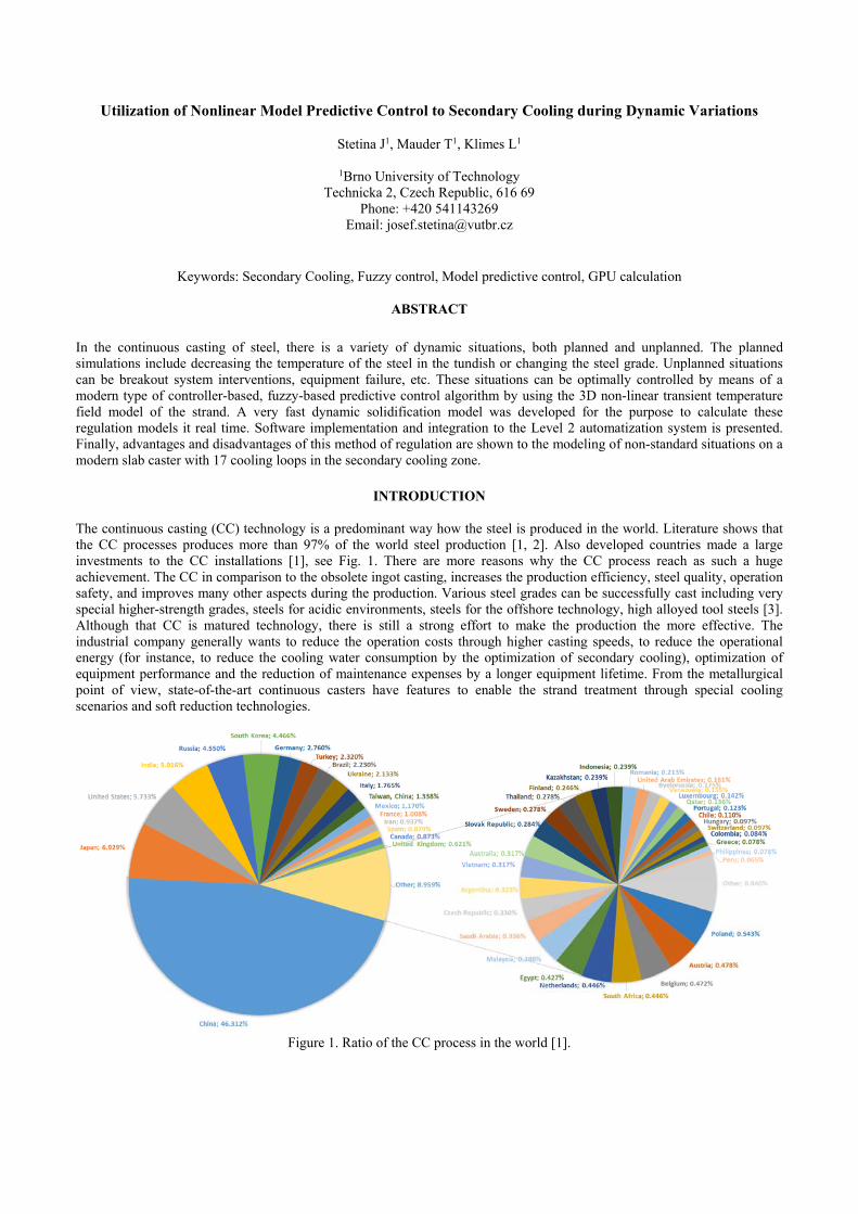
Utilization of Nonlinear Model Predictive Control to Secondary Cooling during Dynamic Variations Stetina J 1 , Mauder T 1 , Klimes L 1 1 Brno University of Technology Technicka 2, Czech Republic, 616 69 Phone: +420 541143269 Email: [email protected] Keywords: Secondary Cooling, Fuzzy control, Model predictive control, GPU calculation ABSTRACT In the continuous casting of steel, there is a variety of dynamic situations, both planned and unplanned. The planned simulations include decreasing the temperature of the steel in the tundish or changing the steel grade. Unplanned situations can be breakout system interventions, equipment failure, etc. These situations can be optimally controlled by means of a modern type of controller-based, fuzzy-based predictive control algorithm by using the 3D non-linear transient temperature field model of the strand. A very fast dynamic solidification model was developed for the purpose to calculate these regulation models it real time. Software implementation and integration to the Level 2 automatization system is presented. Finally, advantages and disadvantages of this method of regulation are shown to the modeling of non-standard situations on a modern slab caster with 17 cooling loops in the secondary cooling zone. INTRODUCTION The continuous casting (CC) technology is a predominant way how the steel is produced in the world. Literature shows that the CC processes produces more than 97% of the world steel production [1, 2]. Also developed countries made a large investments to the CC installations [1], see Fig. 1. There are more reasons why the CC process reach as such a huge achievement. The CC in comparison to the obsolete ingot casting, increases the production efficiency, steel quality, operation safety, and improves many other aspects during the production. Various steel grades can be successfully cast including very special higher-strength grades, steels for acidic environments, steels for the offshore technology, high alloyed tool steels [3]. Although that CC is matured technology, there is still a strong effort to make the production the more effective. The industrial company generally wants to reduce the operation costs through higher casting speeds, to reduce the operational energy (for instance, to reduce the cooling water consumption by the optimization of secondary cooling), optimization of equipment performance and the reduction of maintenance expenses by a longer equipment lifetime. From the metallurgical point of view, state-of-the-art continuous casters have features to enable the strand treatment through special cooling scenarios and soft reduction technologies. Figure 1. Ratio of the CC process in the world [1].
Transcript of Utilization of Nonlinear Model Predictive Control to ... · Utilization of Nonlinear Model...
Utilization of Nonlinear Model Predictive Control to Secondary Cooling during Dynamic Variations
Stetina J1, Mauder T1, Klimes L1
1Brno University of Technology Technicka 2, Czech Republic, 616 69
Phone: +420 541143269 Email: [email protected]
Keywords: Secondary Cooling, Fuzzy control, Model predictive control, GPU calculation
ABSTRACT
In the continuous casting of steel, there is a variety of dynamic situations, both planned and unplanned. The planned simulations include decreasing the temperature of the steel in the tundish or changing the steel grade. Unplanned situations can be breakout system interventions, equipment failure, etc. These situations can be optimally controlled by means of a modern type of controller-based, fuzzy-based predictive control algorithm by using the 3D non-linear transient temperature field model of the strand. A very fast dynamic solidification model was developed for the purpose to calculate these regulation models it real time. Software implementation and integration to the Level 2 automatization system is presented. Finally, advantages and disadvantages of this method of regulation are shown to the modeling of non-standard situations on a modern slab caster with 17 cooling loops in the secondary cooling zone.
INTRODUCTION
The continuous casting (CC) technology is a predominant way how the steel is produced in the world. Literature shows that the CC processes produces more than 97% of the world steel production [1, 2]. Also developed countries made a large investments to the CC installations [1], see Fig. 1. There are more reasons why the CC process reach as such a huge achievement. The CC in comparison to the obsolete ingot casting, increases the production efficiency, steel quality, operation safety, and improves many other aspects during the production. Various steel grades can be successfully cast including very special higher-strength grades, steels for acidic environments, steels for the offshore technology, high alloyed tool steels [3]. Although that CC is matured technology, there is still a strong effort to make the production the more effective. The industrial company generally wants to reduce the operation costs through higher casting speeds, to reduce the operational energy (for instance, to reduce the cooling water consumption by the optimization of secondary cooling), optimization of equipment performance and the reduction of maintenance expenses by a longer equipment lifetime. From the metallurgical point of view, state-of-the-art continuous casters have features to enable the strand treatment through special cooling scenarios and soft reduction technologies.
Figure 1. Ratio of the CC process in the world [1].

Many of these challenges can be solved by using computer heat-transfer, stress-strain and micro-macro segregation numerical models [4, 5, 6]. Computational capabilities have progressed to the point where models used in the CC control include only minor physical simplifications and they can provide more accurate results. The complex 3-D simulations with very fine meshes run even faster than the real time and they can be used for the on-line control of the CC process. Moreover, the numerical models can be supplemented by the optimization, decision-making (optimal control) algorithms and quality control algorithms [7, 8, 9]. An integration of numerical models with optimization algorithms to the level 2 control systems give a general tool for the quality and casting productivity improvement. The basic idea of the paper can be divided into two major parts. The first part deals with the original 3-D heat-transfer-solidification numerical simulation including comprehensive long-term validations on the real slab and billet casters. The second part deals with advanced optimal control tools for the steel quality and the casting productivity improvement. In the first part, a natural effort will be discussed how to accelerate the computation of numerical models in order to improve the applicability for on-line control by using parallelization and computing on graphics processing units (GPUs), the so-called GPGPU programming. The second part will discuss an optimal control algorithm based on the fuzzy logic.
NUMERICAL MODEL OF HEAT TRANSFER AND SOLIDIFICATION
The mathematical formulation of heat transfer and solidification to the temperature distribution and the solid shell profile prediction is based on the governing equation of transient heat conduction, which is also called the Fourier-Kirchhoff equation [4, 9]. The three-dimensional heat transfer can be expressed as
.eff
H Hv k T T
z
(1)
where keff is the effective thermal conductivity (W/m K); T is the temperature (K); H is the volume enthalpy (J/m3); τ is the time (s); v is the casting speed (m/min) and z is the direction of casting (m). For a steady state simulation, the first term at the left hand side in Eq. (1) is zero. Thermophysical properties and IDS The thermophysical parameters such as the thermal conductivity, density, specific heat capacity and the enthalpy are all strong functions of the temperature. Generally there are three common ways how to determine them. Many authors use the empirical relationships which can be applied for certain steel grades and temperature ranges. The second possibility is the real material measurement on small steel samples via Differential thermal analysis or Differential scanning calorimetry. The results are much better than in the previous approach, but the expensiveness of these measurements and a large number of different steel grades cast in CC makes it unacceptable. The last way to estimate thermophysical parameters is the solidification analysis packages. Results of these packages are acceptable and validated for a large range of steel grades. In this paper the thermophysical parameters are computed from the specific chemical composition of the steel by using the solidification analysis package IDS [10]. The IDS (InterDendritic Solidification) is a thermodynamic-kinetic package, which simulates phase changes, compound formation/dissolution and the solute distribution during the solidification of steels and during their cooling /heating process after the solidification. The package also simulates solid state phase transformations related to the austenite decomposition process (ADC) at temperatures below 900/600 °C, and it calculates important thermophysical material properties (enthalpy, thermal conductivity, density, etc.) from the liquid state down to the room temperature. These data are needed in other models, such as in heat transfer and thermal stress models, whose reliability highly depends on the input data itself. The calculations of IDS have been compared with many experimental solidification related measurements showing a good agreement [11]. In order to demonstrate the usability of the presented numerical model, two different type of steels (a low carbon S355JR and a high carbon 30CrNiMo8 steel) were chosen, see Table 1.
Table 1. Chemical composition of the examined grades of steel C Si Mn P Cr Nb V
S355JR 0.11 0.45 1.55 0.075 0 0.02 0 w/% 30CrNiMo8 0.28 0.25 0.45 0.125 1.90 0 0 w/%
S Ni Mo Cu Al Ti Ca S355JR 0.025 0 0 0 0.375 0 0 w/%
30CrNiMo8 0.025 1.90 0.35 0 0.30 0 0 w/% The thermophysical properties for the steel grades S355JR and 30CrNiMo8 determined with the use of IDS are shown in Figures 2 and 3.

Figure 2. IDS results for the steel S355JR.
Figure 3. IDS results for the steel 30CrNiMo8. Initial and boundary conditions In order to have a well-posed problem, initial and boundary conditions must be provided. The initial condition is generally expressed as
0 0, , , , ,T x y z T x y z , (2)
where T0 is the initial temperature distribution in the time τ = 0. Very often the initial temperature is set to the casting temperature Tcast. This is the most common for steady-state simulations. In case of dynamic simulation, the user mostly chooses some already calculated temperature field as initial condition. The determination of the boundary conditions is a more complex issue. Boundary conditions have to be set properly, because boundary conditions highly influence the numerical result. Boundary conditions include the meniscus temperature, heat flux in the mold and under the rollers, forced convection under the nozzles, and free convection and radiation in the tertiary cooling zone. These are mathematically described in Table 2. Table 2. Boundary conditions
Temperature in the meniscus 0, , z castT x y z T
In the exit area 0T
kn
In the mold area
In the secondary cooling zone - nozzles 4 4water amb
Tk htc T T T T
n
In the secondary cooling zone - rollers
In the tertiary cooling zone 44ambambnat TTTThtc
n
Tk

In the Table 2, Twater is the cooling water temperature; Tamb is the ambient temperature; htc is the heat transfer coefficient (W/m2 K); σ is the Stefan-Boltzman constant (W/m2 K4), ε is the emissivity of the slab surface (-), a and b are constants (-), Lk is the length of mould (m). In [5 - 8], a large number of empirical relationships for the determination of boundary conditions through the caster can be found. Unfortunately there is a lack of information such as the rate of water flow in mold walls, the distance and impact angle between the nozzle and the strand surface, influence of the Leidenfrost effect, influence of the strand temperature to the heat transfer coefficient, etc. The more accurate way is the use of laboratory experiments and the operating temperature measurement. The advantage of the model discussed in this paper is that it obtains heat transfer coefficients from measurements of the spraying characteristics of all nozzles used at the caster on a so-called hot plate in the experimental laboratory, see [12]. The experiment is shown in Figure 4 where the nozzle is placed between two rollers and moves under the test plate and sprays the surface. A sufficient range of operational pressures of water and a sufficient range of casting speeds of the strand (i.e. casting speed) were measured. Heat transfer coefficients obtained by the inverse heat conduction problem are entered into a database of boundary conditions from which (based on interpolation) the model determines the appropriate heat transfer coefficient beneath the nozzle for the required temperature of the surface of the slab, the operational pressure of the water, and for the required casting speed. This approach represents a unique combination of experimental measurement in a laboratory and a numerical simulation for the calculation of the non-linear boundary conditions. The measurement part of the research is carried out by Heat and Fluid Flow Laboratory at the Brno University of Technology. Information about the laboratory and the experiment can be found in [12]. The heat transfer coefficient (as well as the heat flux) is calculated using the IHCP (inverse heat conduction problem) from temperatures measured by thermocouples. The IHCP solution does not give the heat transfer coefficient as a continuous function but as a set of discrete values. The objective of the final data processing is to obtain the heat transfer coefficient as a function of position x at a slab and of surface temperature T; htc = f(x,T). A laboratory stand (Fig. 4) developed for testing the nozzles applied for continuous casting was used to test the cooling intensity with the water at elevated temperatures. The tested air-mist nozzles are located under a test plate. The steel frame holds three major parts of the stand: a test plate, a driving mechanism with a nozzle(s) and a heater. The test plate is made of austenitic steel to prevent the surface from a significant oxidation. There are holes drilled into the plate where the thermocouples are placed. The driving mechanism moves the spraying nozzle(s) under the plate. The temperature of 1250 °C was set as the initial temperature. The experiment is finished when the temperature in all the measured points is below 500 °C. An inverse task is used to re-compute the internal temperatures to the surface temperatures in order to obtain the htc.
Figure 4. Laboratory experiment on hot plate (left - thermocouples position, right – the test plate sprayed with nozzles) [12]. Geometric conditions and mesh size In this paper all geometric conditions are taken from the real slab caster with 17 cooling loops in the secondary cooling zone. The loops 1 and 3 influence both the top and the bottom surfaces, while zones 5, 7, 9, 11, 13, 15, and 17 are spraying the top surface and zones 6, 8, 10, 12, 14, and 16 are spraying bottom surface. Only the cooling loop 2 sprays the left and right sides of the strand. Specifications of the slab caster are listed in Table 3. The simulations are carried out for a frequently cast slab cross-section 1400 x 200 mm. Table 3. Caster specifications
Ladle capacity 220 tons Meter weight 1.86 t/m 1,4 t/min No. segments 12 Torch cutting machine type Slab Marking Machine type
Slab width 800-1500 mm Slab thickness 150-210 mm Caster length 26 m Mold length 900 mm Caster radius 8 m No. cooling loops 17 Casting speed 0.9-2 m/min Electrical mold oscillation system

The numerical model has a non-equidistant mesh in all the directions. The reason for this is that the largest temperature gradients are near the surface. In the casting direction the nodes are adapted to the rollers and nozzles positions to get a more accurate determination of boundary conditions. Between the numerical results accuracy (fineness of mesh) and the speed of simulation there has to be a compromise. In the finite difference method, a finer mesh typically results in a more accurate solution. The results should not be affected by the change of the size of the mesh size. The formal method for establishing the mesh convergence requires a curve of a critical result parameter (temperatures) in a specific fixed location, to be plotted against some measure of the mesh density. Several convergence runs were tested. The results in Figure 5 can be used to decide when the convergence is achieved, or how far away the most refined mesh is from the full convergence. The x axis is the number of elements, the y-left axis is the temperature in several points at the top surface (at the end of each cooling circuit) and the y-right axis is the value of the metallurgical length.
Figure 5. Temperatures and metallurgical length for different mesh densities [9]. Software implementation and parallel computation The core of numerical model is programmed in C++ which allows for fast calculations. In cooperation with the IDS, the model allows the user for an application of various enthalpy-temperature functions, thus the temperature field can be calculated for various steel grades via their chemical composition. During the simulation, the Eq. (1) is solved numerically. The explicit schemes easily allow the parallel decomposition. As already mentioned in the introduction, there is a natural effort to speedup numerical models solving the solidification and heat transfer of cast slabs in order to utilize these models for on-line control and regulation of casting process in real time. Currently used commercial dynamic models use traditional single or multi-core CPU computing. However, various computing problems, which can be parallelized, are possible to solve on graphics processing units (GPUs) [13]. These devices, primarily developed for computer graphics acceleration and real-time image rendering, can be used for technical and scientific computing, so-called general-purpose computing on graphic processors (GPGPU). A GPU generally consists of a rather large number (hundreds) of simple cores, which are designed to concurrently execute an identical code but with different data. For computing on GPUs, the parallel computing platform and programming approach are needed. NVIDIA Corporation, which is a forefront manufacturer of GPUs, has developed the Compute Unified Device Architecture (CUDA). The dynamic solidification model presented in the paper was implemented and developed with the use of CUDA C/C++. Nowadays, GPGPU computing is widely used for massively parallel problems, mainly for image processing, Monte Carlo simulations, or molecular dynamics simulations. Several papers were also published in relation to heat transfer problems, see, e.g., [14]. However, the presented usage of GPGPU computing of the dynamic solidification model for continuous casting is rather progressive and has not been published in literature yet. As already described, GPGPU computing is suitable for solving problems with an opportunity for massive parallelism. The described dynamic solidification model belongs among such problems, mainly due to features of the control volume method and due to the explicit time discretization. In order to compare the computing performance, a series of benchmark tests was performed [13]. The CPU-based model was running on a computer with Intel Core 2 Quad processor with four cores of 2.4 GHz and 6 GB RAM memory. The GPU-based model was tested on a computer with the GPU device NVIDIA Tesla C2075, which includes 448 CUDA cores of 1.15 GHz and 6 GB RAM memory. The performance tests were carried out for several number of control volumes of the dynamic solidification model, i.e., for various computing accuracy: from the coarsest grid with 100,000 of control volumes to a finer grid with 5 million of control volumes. Results of computing performance tests are shown in Fig. 6. At the y axis, there is a relative computational time which means that the computing time is divided by the simulated time period. For instance the numerical model with one million nodes is 1.56-times slower than the real time a classic CPU, but on the GPU the simulation runs faster than the real time.

Figure 6. GPU – model benchmarking – relative computational time [13]. As can be clearly seen in Fig. 6, GPU computing allows for a very significant speedup of the dynamic solidification model in comparison to CPU-based computing. The speedup of the model varies with the number of control volumes of the model, i.e., with the density of the mesh, which directly influences the numerical accuracy. For the coarsest grid with 100,000 of control volumes, the speedup provided by the GPU computing is about 30-times in comparison to the CPU computed model. However, when the number of control volumes increases the performance of GPU becomes more evident and the speedup increases as well. For the finer grid with 3 million of control volumes, the speedup is even about 50-times. When we come back to Fig. 5, one can see that if we want to calculate a precise model (at least 2 mil. nodes) in the real time, we have to use GPU computing. Numerical model validation The numerical model of the temperature field without a proper validation cannot be used for the real casting process control. The presented model was validated by surface temperature measurements provided by pyrometers and temperature scanners on the slab and the billet casters [15]. The real history data were selected from castings between 2009 and 2013. The on-line version of the presented numerical model runs in the control system of the slab caster operating in EVRAZ VI´TKOVICE STEEL, a.s. in the Czech Republic and the billet caster operating in Trinecke zelezarny in the Czech Republic. The models were configured for the identical geometry and setup of casting machines [15]. The unevenly oxidized surface of the strand affects the emissivity of the surface and makes the non-contact temperature measurement difficult. Therefore, the data from the pyrometers before the use for the numerical model validation were statistically processed. The median filtering and averaging of measured data through the casting sequence were used. The temperature validation contains a large number of simulations for different steel grades, size of slab, and casting conditions. The temperature field validation for the slab caster is shown in Fig. 7 while for the billet caster in Fig. 8.
Figure 7. Slab caster validation.

Figure 8. Billet caster validation.
FUZZY LOGIC AND MODEL PREDICTIVE CONTROL REGULATION
In order to improve the quality of steel processed on the CC machine, the Fuzzy based controller was created. Unlike classic PID regulators, the Fuzzy regulator gives us better control utilization, higher stability with less overshoots, flexible knowledge base design, fast response on dynamic changes and nonlinear control [16]. An essential aspect of the fuzzy control is the definition and combination of linguistic variables and linguistic rules. Four linguistic variables were created. The "error" presents the temperature difference at a particular control point; the "impact" represents the mean distance between a control point and the adjusting cooling circuit; "total error" is calculated as a sum of all "errors"; and the "metallurgical length" represents the actual position of the solidification point. The linguistic rules are in the form that IF x is A AND y IS B, THEN z IS C. So for instance, IF the actual error of the controlled temperature IS "big" AND the impact IS "big", THEN the modification of cooling intensity IS also "big". Similar fuzzy rules are applied for each circuit and for modification of the casting speed. By the evaluation of these simple rules the optimal values can be found. Membership functions for all linguistic variables are trapezoidal-shaped uniformly distributed through the corresponding intervals. As a defuzzification method the standard center of gravity was chosen. If there is a requirement for a faster reaction, for instance, the on-line regulation case, the user can choose for deffuzification a different method, such as the largest or smallest (absolute) value of maximum. However the regulation will be compressed although less stable. More information about the application of the fuzzy regulator and the detailed description can be found in [9].
Figure 9. Slab caster temperature history at the top and at the bottom surfaces including the allowed temperature intervals.

The steel quality is controlled by keeping the surface and core strand temperatures in the specific ranges corresponding to the hot ductility of steel in order to avoid surface and core defects [17]. Temperatures on the strand surfaces are monitored in specific locations. We call these locations as the “control points”. The inner quality is influenced by the position of the metallurgical length (the length of liquid material from the meniscus). The input for the regulation algorithm is the final temperature field (output from the numerical model), specifically the temperatures in the control points and the value of the metallurgical length. The control points can be placed anywhere at the strand surface. The control of secondary cooling is divided into several cooling loops (17 in this case) and, from the regulation point of view, the most “interesting” surface temperatures are in front of and behind the circuits. In the presented case, the control points are placed behind each circuit, which also helps to easily create the linguistic rules and the linguistic variables for fuzzy logic decisions. The example of temperature intervals and the average surface temperature which satisfies these intervals can be seen in Fig. 9. The numerical model allows us to calculate the future states of the temperature field. In combination with the fuzzy regulator, the model-based predictive control (MPC) can be created. Though primarily utilized in the petroleum industry, the model-based predictive control has been recently used in many engineering application, mainly due to a rapid development of computers and their performance [18, 19]. The MPC utilizes the model of the process to predict the behavior of the system resulting from the changes in the inputs and to evaluate the consequences of these modifications. We deal with the Scenario approach where the fuzzy regulator picks the best solution. The Scenario approach in this situation means to recalculate the solidification model many times, which increases the computational time significantly. However, by using the developed very fast GPU numerical model the Fuzzy-Model predictive control (F-MPC) brings elegant, robust and powerful solution how to optimally control the CC process.
INTEGRATION OF THE F-MPC-NUMERICAL MODEL TO LEVEL 2 AUTOMATIZATION SYSTEM
An integration of the discussed F-MPC-numerical model to the Level 2 automatization system is carried out in the cooperation with ASM Automation Company (www.asmautomation.com). ASM Automation was founded in 1999 in Germany and the company is focused on providing services in industrial automation. In 2008 the company expanded into the Czech Republic. At present the company has 4 branches located in two countries where experienced specialists take care of the projects. Since the beginning of its existence, the company ASM Automation supplies a complex solution of industrial automation, especially for foundries and steel mills. The company developing original software products and offers the custom software development according to customer requirements. Flagship product is the Level 2 process automation system (Level 2) for Electric Arc Furnaces (EAF), Ladle Furnaces (LF) and Continuous Casting Machines (CCM).
Figure 10. Block scheme of software implementation.
Level 2 is a modular system. Individual modules can be modified or added based on customer specifications for adjusting a particular operation - we offer made-to-measure solutions to our clients. The customers can use a fat-client Level 2 application with an auto update utility or a web browser based client for remote control. In June 2014, the cooperation with Brno University of Technology (BUT) started to implement a more precise metallurgical model (Dynamic Solidification Model) for CCM into our Level 2 system. We also offer the Breakout prevention system. Depending on the wish of customer we can also deliver different metallurgical models for EAF and LF.

Main goals of the system are to decrease the tapping temperature of EAF, to decrease the melting and refining time of EAF and LF, precise calculation of energy, temperature, alloys and costs + optimized metallurgical models for EAF, LF and CCM. Last but not least aim is to increase the total productivity and quality. The overall software implementation is shown as a block scheme in Fig. 10. The client part of the presented numerical model interface (called Brno Dynamic Solidification Model) has a simple style and can be also operated using touch control. The part of user interface can be seen in Fig. 11.
Figure 11. Numerical model interface.
RESULTS AND DISCUSSION
The fuzzy regulator was tested for many different fuzzy parameters, for different temperature and casting speed constraints, for different caster and slab geometries, and for different steel grades. This section shows an example of the setting of constraints and related results. The first scenario simulates 1 hour casting process where a drop of the casting from 1.9 to 1.2 m/min at 30 min and the increase of the casting speed from 1.2 to 1.9 m/min occurs at time 40 min, see Fig. 12. The simulation is provided for three cases; first case simulates a situation without a regulation intervention, in the second case the fuzzy regulation is applied while the third one is the case where the F-MPC regulator is used. The simulations are provided for the caster with 17 cooling zones described in Table 3.
Figure 12. Casting speed for the test case.
Table 4. Temperature limits in °C for 16 regulation points
RP 1 2 3 4 5 6 7 8 9 10 11 12 13 14 15 16
Lower 1200 1100 1010 1010 960 960 950 950 920 920 890 890 850 850 820 820

limit
Upper limit
1400 1212 1122 1122 1050 1050 1020 1020 990 990 952 952 930 930 921 921
For this caster 16 controlled points has been placed after cooling zones on the top and bottom surface. The allowed temperature interval for these 16 controlled points are shown in Table 4 and Fig. 9. For each control strategy two figures are presented: the time-dependent water flow volumes through all cooling circuits, and the time-dependent temperature errors that evaluate the control process. The results are shown in Fig. 13 – 15.
Figure 13. Case with no regulation: left-Water flow volumes, right - Surface temperature errors
Figure 14. Case with fuzzy regulation: left-Water flow volumes, right - Surface temperature errors
Figure 15. Case with fuzzy-MPC regulation: left-Water flow volumes, right - Surface temperature errors
The second scenario simulates a change of steel grade S355JR to steel grade 30CrNiMo8 (Tab. 1). The casting speed is constant of 1.9 m/min. The simulation was again carried out for three cases; first case simulates a situation without the regulation intervention, in the second case the fuzzy regulation is applied while the third one is the case where the F-MPC regulator is used. The allowed temperature intervals are the same as in the case one (Table 4). The results of simulations can be seen in Fig. 16 - 18.

Figure 16. Case with no regulation: left-Water flow volumes, right - Surface temperature errors
Figure 17. Case with fuzzy regulation: left-Water flow volumes, right - Surface temperature errors
Figure 18. Case with fuzzy-MPC regulation: left-Water flow volumes, right - Surface temperature errors
In order to compare the execution times, both the regulators were calculated on the single CPU. Average execution time for 1 hour simulation (testing cases) with the fuzzy controller was approximately 27.25 min, while using the F-MPC controller simulation takes 47.20 min. It was also mentioned above that using the MPC prolongs the computation time. In case that all these simulations should be calculated for the finer meshes, using the GPU model would be necessary in order to have results faster than the real time. The F-MPC reached very good results, the temperature errors are negligible in comparison with the fuzzy control or with the situation without the regulation. However there is one attribute in which the classic fuzzy regulator has a better behavior than the F-MPC. The fuzzy control has smoother reaction that the F-MPC, see Fig. 13 - 18 left. The prediction was set to the future time 15 sec. This interval can be longer which will smooth the results. On the other hand the temperature errors can be larger. The user has to set some compromise between smoothness of control and temperature errors.
CONCLUSIONS
The paper presents the use of advanced 3D transient numerical heat transfer model, its extension to the GPU calculation, validation for slab and billet casters and the possibility for advanced control algorithms based on the fuzzy logic and the model predictive control (and their combination) for the regulation of secondary cooling. The numerical model is general by using the IDS solidification model and is highly accurate due to extensive nozzle measurements in the Heat and Fluid Flow Laboratory. Massive parallelization on the GPU allows us to calculate numerical models with millions of nodes faster than the real time. The cooperation with ASM Automation Company presents a very elegant solution how to integrate the

mentioned model to the Level 2 automation system. Moreover, to increase the quality of steel, the fuzzy regulator was created to establish appropriate cooling intensities for different casting speeds and casting temperature conditions; to optimally react to dynamic changes of process parameters; and to avoid and prevent liquid steel breakouts by monitoring the position of the metallurgical length. The regulator was tested for different casting conditions and parameter setting. The main advantage is a small number of evaluations to find the optimal solution. As an extension, original MPC was connected to the fuzzy regulator (FMPC) in order to get even better results. The calculation with the MPC prolong the execution time but in combination with the GPU numerical model, the optimal regulation can be found faster than the real time. This solution brings the real-time regulator which can efficiently solve dynamic changes which occur in the real CC process. The system concept was universally designed to optimally control any slab or billet CC process and can be used for maximizing the productivity and increasing the final steel quality.
ACKNOWLEDGEMENTS The presented research was supported by the NETME+ project (LO1202) with the financial support from the Ministry of
Education, Youth and Sports of the Czech Republic under the “National Sustainability Programme I” and by the TG01010054 project of the Technology Agency of the Czech Republic.
REFERENCES
1. Dahmen, B.,Economical and flexible tailor-made solutions for the production of new steel grades, In METEC & 2nd ESTAD 2015 Proceedings. 1. Dusseldorf: Steel Institute VDEh, 2015. s. 1-8. ISBN: 978-3-00-049542- 7
2. Sulaiman H. Steel in automotive industry– the view from the supply chain, In METEC & 2nd ESTAD 2015 Proceedings. 1. Dusseldorf: Steel Institute VDEh, 2015. s. 1-8. ISBN: 978-3-00-049542- 7
3. K. Mouralova, J. Kovar, Quality of Dimensions Accurancy of Components After Wedm Depending on The Heat Treatment. MM Science Journal, 2015, Vol. 4, pp. 790-793. ISSN: 1803- 1269.
4. D.M. Stefanescu: Science and Engineering of Casting Solidification, Second Edition, 2009, New York, Springer Science, p. 402.
5. H. Wang, et al.: ISIJ International, 2005, vol.45(9), pp-1291-1296. 6. S. Louhenkilpi, et al.: Materials Science and Engineering A, 2005, 413–414, pp. 135 – 138. 7. J. Zhemping, et al.: Proceedings of the 2007 IEEE International Conference on Integration Technology, 2007,
Shenzhen, China: IEEE, pp. 558 – 562. 8. P. Zheng, J. Guo, and X.J. Hao: IEEE International Conference on Industrial Technology, 2004, Hammamet, Tinisia:
IEEE, pp. 1156 - 1161. 9. T. Mauder, C. Sandera, J. Stetina, Optimal control algorithm for continuous casting process by using fuzzy logic, Steel
Res. Int., 2015, Vol. 86(7), pp. 785-798, DOI: 10.1002/srin.201400213. 10. J. Miettinen: Brief Description of Solidification Package IDS: User manual, 2015, Casim Consulting Oy Espoo,
Finland, p. 16. 11. J. Miettinen: Validation of IDS calculations with experimental data, Project report, 2015, Aalto University, Finland, p.
19. 12. M. Raudensky, M. Hnizdil, J. Hwang, S. Lee, and S. Kim: Materiali in tehnologije, 2012, vol. 46(3), pp. 311 - 315. 13. L. Klimes, and J. Stetina: Conference proceedings of 22nd Conference on metallurgy and materials, 2013, Ostrava,
Tanger, s.r.o. pp. 34 - 39. 14. FU, W. S., WANG, W. H., HUANG, S. H. An investigation of natural convection of three dimensional horizontal
parallel plates from a steady to an unsteady situation by a CUDA computation platform. International journal of heat and mass transfer, 55 (2012) 17-18, pp. 4638-4650.
15. J. Stetina, F. Kavicka, T. Mauder, L. Klimes. Transient simulation temperature field for continuous casting steel billet and slab. In METEC InSteelCon 2011. Dusseldorf, Německo, TEMA Technologie Marketing AG. 2011. p. 13 - 22.
16. L. Klimes, T. Mauder, J. Stetina Comparison of regulation algorithms for secondary cooling of continuous casting process. In Proceedings of METAL 2015. Ostrava, TANGER Ostrava, s.r.o. 2015. p. 39 - 44. ISBN 978-80-87294-58-1.
17. G.S. Jansto: METAL 2013 Conference proceedings, 2013, Ostrava, Tanger s.r.o. pp. 32 - 39. 18. L. Klimes, J. Stetina: Materiali in tehnologije, 2014, vol.48(4), pp. 525-530 19. A. Ivanova. Model predictive control of secondary cooling model in continuous casting. In METAL 2013: 22nd
International Conference on Metallurgy and Materials. Ostrava: TANGER, 2013, pp. 81–86.