UTILIZATION OF A TIME DOMAIN SIMU ...
114
Risto Tiainen UTILIZATION OF A TIME DOMAIN SIMU- LATOR IN THE TECHNICAL AND ECONOMIC ANALYSIS OF A WIND TURBINE ELECTRIC DRIVE TRAIN Thesis for the degree of Doctor of Science (Technology) to be presented with due permis- sion for public examination and criticism in the Auditorium of the Student Union House at Lappeenranta University of Technology, Lappeenranta, Finland, on the 13 th of August, 2010, at noon. Acta Universitatis Lappeenrantaensis 391
Transcript of UTILIZATION OF A TIME DOMAIN SIMU ...

Risto Tiainen
UTILIZATION OF A TIME DOMAIN SIMU-LATOR IN THE TECHNICAL AND ECONOMICANALYSIS OF A WIND TURBINE ELECTRICDRIVE TRAIN
Thesis for the degree of Doctor of Science(Technology) to be presented with due permis-sion for public examination and criticism inthe Auditorium of the Student Union Houseat Lappeenranta University of Technology,Lappeenranta, Finland, on the 13th of August,2010, at noon.
Acta UniversitatisLappeenrantaensis391

Supervisors Professor Jero AholaLappeenranta University of TechnologyFinland
Dr. Tuomo LindhLappeenranta University of TechnologyFinland
Reviewers Professor Kimmo KauhaniemiUniversity of VaasaFinland
Dr. Jouko NiiranenABB DrivesFinland
Opponents Professor Kimmo KauhaniemiUniversity of VaasaFinland
Dr. Jouko NiiranenABB DrivesFinland
ISBN 978-952-214-947-3ISBN 978-952-214-948-0 (PDF)
ISSN 1456-4491
Lappeenrannan teknillinen yliopistoDigipaino 2010

Abstract
Risto Tiainen
Utilization of a Time Domain Simulator in the Technical and Economic Analysis of aWind Turbine Electric Drive Train
Dissertation, Lappeenranta University of Technology109 p.Lappeenranta 2010ISBN 978-952-214-947-3, ISBN 978-952-214-948-0 (PDF)ISSN 1456-4491
The amount of installed wind power has been growing exponentially during the past tenyears. As wind turbines have become a significant source of electrical energy, the interactionsbetween the turbines and the electric power network need to be studied more thoroughly thanbefore. Especially, the behavior of the turbines in fault situations is of prime importance;simply disconnecting all wind turbines from the network during a voltage drop is no longeracceptable, since this would contribute to a total network collapse. These requirements havebeen a contributor to the increased role of simulations in the study and design of the electricdrive train of a wind turbine.
When planning a wind power investment, the selection of the site and the turbine are crucialfor the economic feasibility of the installation. Economic feasibility, on the other hand, is thefactor that determines whether or not investment in wind power will continue, contributingto green electricity production and reduction of emissions. In the selection of the installationsite and the turbine (siting and site matching), the properties of the electric drive train ofthe planned turbine have so far been generally not been taken into account. Additionally, al-though the loss minimization of some of the individual components of the drive train has beenstudied, the drive train as a whole has received less attention. Furthermore, as a wind turbinewill typically operate at a power level lower than the nominal most of the time, efficiencyanalysis in the nominal operating point is not sufficient.

This doctoral dissertation attempts to combine the two aforementioned areas of interest bystudying the applicability of time domain simulations in the analysis of the economic feasibil-ity of a wind turbine. The utilization of a general-purpose time domain simulator, otherwiseapplied to the study of network interactions and control systems, in the economic analysisof the wind energy conversion system is studied. The main benefits of the simulation-basedmethod over traditional methods based on analytic calculation of losses include the abil-ity to reuse and recombine existing models, the ability to analyze interactions between thecomponents and subsystems in the electric drive train (something which is impossible whenconsidering different subsystems as independent blocks, as is commonly done in the analyt-ical calculation of efficiencies), the ability to analyze in a rather straightforward manner theeffect of selections other than physical components, for example control algorithms, and theability to verify assumptions of the effects of a particular design change on the efficiency ofthe whole system.
Based on the work, it can be concluded that differences between two configurations can beseen in the economic performance with only minor modifications to the simulation modelsused in the network interaction and control method study. This eliminates the need of devel-oping analytic expressions for losses and enables the study of the system as a whole instead ofmodeling it as series connection of independent blocks with no loss interdependencies. Threeexample cases (site matching, component selection, control principle selection) are providedto illustrate the usage of the approach and analyze its performance.
Keywords: Wind power, simulation, technical and economic analysisUDC 621.548:621.311.245:004.94.003

Acknowledgments
The research documented in this thesis was carried out at the Institute of Energy Technology(LUT Energia) at Lappeenranta University of Technology (LUT) during the years 2008–2009.The research was partly funded by the Graduate School of Electrical Engineering (GSEE) andThe Switch Ltd.
I would like to thank the people I have had the pleasure of working with at the University.Especially my supervisors, Professor Jero Ahola and Dr. Tuomo Lindh, and my former col-league, Dr. Ville Särkimäki, deserve a big thank you. You have been an inexhaustible sourceof ideas, comments, and (constructive) criticism over the years.
I would also like to thank the pre-examiners of this thesis, Professor Kimmo Kauhaniemiand Dr. Jouko Niiranen, for their valuable comments and corrections during the preparationof this thesis. Many of your comments gave me new insight on the topics discussed in thisbook.
Furthermore, the contribution of Dr. Hanna Niemelä, who helped me rid the manuscript ofall of those recurring mistakes I tend to make with my English, is sincerely acknowledged.
When working in an academic environment, the work pace is sometimes hectic. More oftenthan not, however, there is time for lengthy coffee breaks. These breaks, if spent with a goodcoffee-drinking squad, provide an excellent chance to get new ideas and to broaden yourthinking. I had the pleasure to take part in many such occasions, and I would like to thank allthose colleagues who used to sit around the round table with me.
The financial support by the Walter Ahlström Foundation, the Jenny and Antti Wihuri Foun-dation, the Lahja and Lauri Hotinen Fund, and the Ulla Tuominen Foundation is greatlyappreciated.
Finally, I would like to express my gratitude to my family. Especially I’d like to thank you,Tiina, my dear fiancée, for bearing with me when I was sitting by the computer writing forthe most of the day and just acting grumpy for the rest of the day. Or deriving equations inthe middle of the night. I wish I could guarantee that this won’t happen ever again, but I’m

afraid I can’t. But I’m also sure we’ll pull through just fine.
Lappeenranta, May 31st, 2010
Risto Tiainen

Contents
Symbols and Abbreviations 9
1 Introduction 131.1 Motivation of the Research . . . . . . . . . . . . . . . . . . . . . . . . . . . 141.2 Objective of the Research . . . . . . . . . . . . . . . . . . . . . . . . . . . . 181.3 Outline of the Thesis . . . . . . . . . . . . . . . . . . . . . . . . . . . . . . 181.4 Scientific Contribution of the Thesis . . . . . . . . . . . . . . . . . . . . . . 19
2 Development of the Analysis Method 212.1 Introduction to Wind Power . . . . . . . . . . . . . . . . . . . . . . . . . . . 212.2 Wind Turbine Annual Energy Output . . . . . . . . . . . . . . . . . . . . . . 23
2.2.1 Power of Wind . . . . . . . . . . . . . . . . . . . . . . . . . . . . . 232.2.2 Wind Turbine Output Power . . . . . . . . . . . . . . . . . . . . . . 242.2.3 Wind Statistics . . . . . . . . . . . . . . . . . . . . . . . . . . . . . 272.2.4 Calculating the AEO . . . . . . . . . . . . . . . . . . . . . . . . . . 30
2.3 Regulations Relevant to Wind Power . . . . . . . . . . . . . . . . . . . . . . 352.3.1 International and European Standards . . . . . . . . . . . . . . . . . 362.3.2 Transmission System Operator Requirements . . . . . . . . . . . . . 37
2.4 Investment Analysis . . . . . . . . . . . . . . . . . . . . . . . . . . . . . . . 392.4.1 Components of the Analysis . . . . . . . . . . . . . . . . . . . . . . 392.4.2 Common Analysis Methods . . . . . . . . . . . . . . . . . . . . . . 402.4.3 Analysis Using the Present Value Method . . . . . . . . . . . . . . . 412.4.4 Supplementing the Analysis with the Payback Time . . . . . . . . . . 462.4.5 Implemented Tools . . . . . . . . . . . . . . . . . . . . . . . . . . . 48
2.5 Summary . . . . . . . . . . . . . . . . . . . . . . . . . . . . . . . . . . . . 50
3 Simulations in the Wind Turbine Technical and Economic Analysis 513.1 Introduction . . . . . . . . . . . . . . . . . . . . . . . . . . . . . . . . . . . 513.2 Calculation of Powers and Losses . . . . . . . . . . . . . . . . . . . . . . . 523.3 Modeling the Losses in the Simulation . . . . . . . . . . . . . . . . . . . . . 54
3.3.1 Generator . . . . . . . . . . . . . . . . . . . . . . . . . . . . . . . . 583.3.2 Filters . . . . . . . . . . . . . . . . . . . . . . . . . . . . . . . . . . 593.3.3 Power Electronic Converter . . . . . . . . . . . . . . . . . . . . . . 603.3.4 Transformer . . . . . . . . . . . . . . . . . . . . . . . . . . . . . . . 62
3.4 Example Cases . . . . . . . . . . . . . . . . . . . . . . . . . . . . . . . . . 62

3.4.1 Case 1: Component Selection . . . . . . . . . . . . . . . . . . . . . 623.4.2 Case 2: Electric Drive Train Sizing . . . . . . . . . . . . . . . . . . 713.4.3 Case 3: Drive Train Control Evaluation . . . . . . . . . . . . . . . . 813.4.4 Discussion . . . . . . . . . . . . . . . . . . . . . . . . . . . . . . . 85
4 Conclusion and Discussion 87
Appendices 91
A Loss Calculation over a Three-Phase Component 93
B Wind Distribution Graphs 97
References 103

List of Symbols and Abbreviations
Roman Letters
A AreaA State vectorCi Investment costComr Operations, maintenance, and repair costsCp Wind turbine power coefficientc Weibull distribution scale parameterD DiameterE EnergyEao Annual energy output (AEO)F (v) Weibull cumulative distribution functionfnom Nominal frequencyJ Incomek Weibull distribution shape parameterN Number of binsnnom Nominal rotation speed (revolutions per minute)P Active powerPe Electrical powerPw Power of windPw Average power of windp Instantaneous power; Interest rate; Number of pole pairsp(v) Weibull probability density functionQ Reactive powerr RadiusS Scrap value, salvage valueT Turbine lifeTTT e Electrical torque (space vector)Tpb Payback timet Timet0 Initial time indexu Voltage (instantaneous value)

v, vw Wind speed (scalar)v Average wind speed (scalar)vcut−in Cut-in speed of a wind turbinevcut−out Cut-out speed of a wind turbine
Greek Letters
Γ (x) The gamma functionη Efficiencyλ Tip speed ratioπ Average price of electricityρ Density of airψψψs Stator flux linkage (space vector)ω Angular frequency
Subscripts
e Electricalm, mech Mechanicaln, nom Nominalopt Optimalt Turbinew Wind
Acronyms
AEO Annual Energy OutputCDF Cumulative Density FunctionCOE Cost of EnergyDD Direct DriveDFIG Doubly Fed Induction GeneratorDFT Discrete Fourier TransformEMC Electromagnetic CompatibilityESR Equivalent Series ResistanceESL Equivalent Series Inductance

FEM Finite Element MethodFRT Fault Ride-ThroughHAWT Horizontal-Axis Wind TurbineHV High VoltageIEA International Energy AgencyIEC International Electrotechnical CommissionIGBT Insulated Gate Bipolar TransistorLV Low Voltage (<1000 V)MPPT Maximum Power Point TrackingMV Medium VoltageOECD Organization for Economic Co-operation and DevelopmentOMR Operations, Maintenance, and RepairPCC Point of Common CouplingPDF Probability Density FunctionPM Permanent MagnetPMSG Permanent Magnet Synchronous GeneratorRPM Revolutions per MinuteTSO Transmission System OperatorVSI Voltage Source InverterWECS Wind Energy Conversion SystemWWEA World Wind Energy Association


13
Chapter 1
Introduction
Wind was one of the first sources of energy taken into use by man. It was used as an alterna-tive to human or animal power, for example in grinding grain and pumping water. After thetechnological advances in the 18th and 19th centuries, however, wind power gave way to moreeasily controllable and predictable means of power production, such as coal-powered steamengines and hydroelectric generators. Interest in wind energy was renewed in the 1960s and70s along with an increase in general awareness of environmental protection – and an increasein the price of oil.
Although some (not very successful) megawatt-class turbines were built in the 1970s, earlymodern wind turbines were typically small in today’s terms. In the early 1980s, the nominalpower of wind turbines was typically around 50 kW. The applied technology was furtherdeveloped and upscaled. In the mid-1990s, the nominal power of new wind turbines hadalready reached the next order of magnitude, being approximately 500–750 kW (Neij, 1999).Since then, upscaling has continued, and modern utility-scale wind turbines have commonlya nominal power of 1 MW or more.
The installed wind power capacity is constantly growing. After the year 2000, the annualincrease in total installed wind power capacity1 has been approximately 25–30 % (WWEA,2008, REN21, 2008). However, globally, the total electrical energy production from windis still small compared with many other sources: approximately 1 % of global electricityproduction comes from wind generators (WWEA, 2008). Potential for further growth exists.Hoogwijk et al. (2004) estimate the global technical potential of on-shore wind energy tobe approximately six times the current global electricity consumption. Archer and Jacobson(2005) arrive at similar figures.
The approximately one percent of the world’s electricity generation by wind turbines is notthe whole picture. This wind energy production is very unevenly distributed over the surfaceof the planet. 73 % of the installed global wind power capacity was located in Europe in
1The sum of the nominal powers of all installed turbines

14 Introduction
2004, Germany being the largest single contributor (17 GW, 49 % of the total Europeancapacity) and Denmark being the country with the largest percentage (20 %) of electricitydemand covered by wind power production (Hansen and Hansen, 2006). The European coastis one of the most favorable sites for wind power production (Archer and Jacobson, 2005).However, increasing wind power capacity has thus far also necessitated economic incentives.Tariff-based remuneration systems for wind power in otherwise liberalized electricity marketshave generally been successful. On the other hand, lack of stable conditions for investmentin wind power may be a significant obstacle to major adoption of wind turbines. This hasbeen the case in, for example, the United Kingdom, which is one of the windiest countriesin Europe and yet has only a modest amount of wind power capacity (Ibenholt, 2002). Thiskind of economic supportive measures by the government often also have an impact on thedevelopment of wind power industry in a country, as concluded by Lewis and Wiser (2007).The leading wind turbine manufacturers come from countries with significant wind powerproduction; the four manufacturers with the greatest market share were in 2004 Vestas (34 %world market share; Denmark), Gamesa Eolica (17 %; Spain), Enercon (15 %; Germany),and GE Wind (11 %; USA) (Hansen and Hansen, 2006).
Thus, economic factors play a key role in the increase in wind power generation. Tradition-ally, the feasibility of a planned wind power installation is evaluated by calculating the costof producing a kilowatt-hour of electricity (see e.g. (Tande and Hunter, 1994)). This figurecan then be used to compare the wind power-based system with another power source (forexample, a diesel-powered system in Lysen (1983, Section 12)), another wind turbine, oranother location for the same turbine. The latter two are called wind turbine site matchingand siting, respectively. Studies of this kind have been widely published, for example byRehman et al. (2003), Rehman and Ahmad (2004), Ucar and Balo (2009b,a), Ahmed Shataand Hanitsch (2008), Jowder (2009). The studies referenced do not go into the details of thewind turbine drive train. Instead, they treat the turbines as ”black boxes”, where the outputelectrical power of the turbine system equals the mechanical power captured by the turbine.In reality, the efficiency of the electric drive train is not unity and not even constant but afunction of the operating point (wind speed).
Regarding the turbine system as a black box, as described above, is often sufficient whenselecting the most suitable site for a turbine or selecting the power rating of a planned system.However, this kind of an analysis is of no help to a manufacturer of wind turbine drive trainelectric components (such as generators and converters) when selecting these components andtheir parameters, or control algorithms. This kind of an analysis and optimization has beencarried out by deriving analytical expressions for the efficiency of subsystem components by,for example, Grauers (1996), Polinder et al. (2006), Li and Chen (2007).
1.1 Motivation of the Research
The economic feasibility of a turbine is, as discussed, of prime importance. Wind powertechnology is constantly developing, and there are multiple technologies for the conversionof mechanical rotation energy of the turbine into electrical energy. The selection of drive

1.1 Motivation of the Research 15
train components and their parameters involves thus quite a lot of work. Optimally, theconfiguration selected is the one which provides the lowest cost of energy while meeting alltechnical requirements. These technical requirements include, for example, fault tolerance(or, fault ride-through, FRT, capability). FRT capabilities of wind turbines are of increasingimportance as the level of wind power penetration in power systems increases. In many cases,the fulfillment of FRT requirements is tested and verified using simulations (see (Luukkoet al., 2009b)). The fault ride-through capability (especially in full power converter-baseddrives) can be affected by electrical and control design, and, therefore, there often exists asimulation model of the electric drive train.
Knowing the difficulties related to the analytic calculation of losses and knowing that thereoften exist simulation models of the electric drive train of a wind turbine system suggest thatit might be feasible to combine the economic feasibility study (e.g. siting, site matching)and the technical simulation models into a technical and economic analysis of the feasibil-ity of a proposed wind turbine system. This kind of a system would eliminate the need todevelop any additional loss models and yet be able to analyze the feasibility of a given com-ponent or subsystem selection compared with others, thereby including the contribution ofdiffering technical selections in the economic analysis. In practice, by adopting this kind ofan approach, a wind power manufacturer or a technology integrator with existing simulationmodels of their technology could with relatively little effort show a potential customer (windpower investor) the effect of alternative technical selections on the economy of the candidatesystems in various wind conditions.
Analytical calculation of losses has at least two downsides. First of all, analytical calculationof losses in multiple operating points is far from straightforward even for a single component.Secondly, and perhaps more importantly, considering components of the drive train indepen-dently fails to take into account the possible effects of parameter selections in one part of thedrive train on the losses of another part of the same drive train. The effects are often such thatthey demand an iterative solution. For example, changing the components of the generatorfilter will change the voltages in the generator terminals, which will change the generatorstator copper losses, which will change the stator current, which will change the losses in thegenerator filter, which will change the voltages in the generator terminals, and so on. The ef-ficiency of the series connection of elements is not generally the product of the efficiencies ofthe individual components measured independently of the series connection. In other words,the efficiency of a single component (or subsystem) is not a constant, but rather a function ofthe operating point of the component. Furthermore, the operating point can be defined to bedetermined by the vectors of state variables (currents and voltages) of both the input and theoutput terminals,
ηi = f (Ain,i,Aout,i) , (1.1)
where ηi is the efficiency of component i, Ain,i is the vector of state variables for the inputport of component i, and Aout,i is the vector of state variables for the output port of componenti. The dependency of the efficiency of a component of the states of the input and output ports(the function f ) can be determined by, for example, laboratory measurements, or simulations.
When multiple components are connected in series (or in parallel), the states of the portsof a component are no longer independent of the other components. The efficiency of the

16 Introduction
total system is not generally equal to the product of the efficiencies of individual componentsdetermined independently of the whole system. Figure 1.1 illustrates the case.
Comp. 1
η1
Comp. 2 Comp. 3
Comp. 1 Comp. 2 Comp. 3
η1 η2 η3+ +η =
a)
b)
Ain,1 Aout,1 Ain,2 Aout,2 Ain,3 Aout,3
Ain,1 Aout,1 Ain,2 Aout,2 Ain,3 Aout,3= =
=f1(Ain,1,Aout,1) η2=f2(Ain,2,Aout,2) η3=f3(Ain,3,Aout,3)
Fig. 1.1. Efficiency of a component is a function of the states of its input and output (a). When connect-ing components in series (b), each individual component is no longer independent. The total efficiencyof the series connection is not generally equal to the product of the efficiencies of individual componentsmeasured (or calculated, or simulated) independently of the whole system.
Simulations are a useful tool in the determination of the states of the subsystem interfacesin a complex system, something which is far from straightforward using analytic methods.With simulation models that accurately model all relevant loss mechanisms and componentinteractions, the total system efficiency can be determined with good accuracy. Thus, a sig-nificant benefit of the simulation-based approach over analytic methods is the fact that thestates of the inputs and outputs of all components in a system can be determined in a rel-atively straightforward way. Additionally, determining the efficiency of a component as afunction of the states of its input and output can also be more straightforward than using an-alytic methods. Since a change improving the performance of a component could actuallyresult in degraded performance of the whole system, finding the total economic optimum forthe drive is downright impossible without considering the drive train as a whole.
In addition to taking into account some of the interactions between the constituent compo-nents of the drive train, the effects of different control principles are more straightforwardto analyze with a simulator than by using analytical modeling. For example, the economicperformance of different modifications to the standard id = 0 control of a permanent magnetgenerator could be compared. Furthermore, the effects of these modifications to the technicalperformance (FRT, for example) could be checked with the same simulator. Also, if a selec-tion or change is assumed to have a certain effect on the economic performance of the plant

1.1 Motivation of the Research 17
(assumed improvement of efficiency, for example), the simulator can be used to check andverify the assumption.
A disadvantage of the simulation-based approach compared with analytic calculation couldbe the required simulation time, which is often several hours, while the values of the an-alytical expressions can be calculated almost instantaneously. However, the time requiredto develop the simulation models could be short compared with time needed for developinganalytic expressions, especially if simulation models already exist for purposes other thanefficiency analysis. Furthermore, multiple simulations can be calculated in parallel (on mul-tiple computers), and the calculation requires no human intervention thereby enabling thedesigner to do other work while the analyses are being calculated. Tools developed duringthis project are specifically designed so that they require no user intervention during the sim-ulation process (for example starting the simulation for multiple operating points, storing theresults).
The traditional cost of energy (COE) based comparison metric of alternative configurationsis very illustrative in many cases (for example, when comparing a wind turbine with a dieselgenerator). However, in the analysis of the electric drive train, there might arise situationsin which this metric is not very descriptive. An example could be the selection of a filtercore material; one of them has lower iron losses than the other, but is also more expensive.The designer can analyze both configurations in some wind conditions and get the COE ofboth configurations and select the more feasible one. However, if the question is insteadformulated ”How much more can the better core cost in order to still be more feasible inthese wind conditions?”, then the COE does not give a direct answer. Therefore, in this work,an alternative method for assessing and comparing wind turbine systems was developed.
The use of a simulator enables various different types of technical and economic analyses tobe performed that are not possible by an analytical approach. The cost of the method is theneed for simulation models. However, the models might already exist for other purposes. Theimprovement and even optimization of the economic efficiency of wind energy productionwould presumably make the investment in wind power more feasible, thus contributing to anincrease in renewable energy production. This work attempts to test the applicability of thesimulation-based approach in the technical and economic analysis of wind power and to findits benefits and limitations. To the best of the author’s knowledge, the use of a simulation-based approach in the technical and economic analysis has not been proposed before.
Figure 1.2 presents the position of the work at hand in relation to siting and COE-related anal-yses, and the simulations used for FRT capability development. The simulator is a tool thatcan be used in both the technical and the economic analysis and to analyze interconnectionbetween the two worlds.

18 Introduction
Fig. 1.2. This work combines traditional siting and COE (cost of energy) analysis with simulations usedin FRT (fault ride-through) studies.
1.2 Objective of the Research
The objective of the study was to analyze the usability of a time domain simulator in thetechnical and economic analysis of a wind turbine electric drive train. In addition to sitingand site matching, the simulation-based method was expected to be applicable to the selectionof the components and parameters of the electric drive train of the turbine, something whichis not straightforward using the more conventional analytical calculation based on models ofthe individual subsystems. In the work, the utilization of the simulator is studied at a generallevel and with the help of example cases.
1.3 Outline of the Thesis
The remaining parts of this doctoral dissertation are organized to chapters as follows.
Chapter 2 introduces the boundary conditions inside which the wind turbine designer oper-ates. First, the power of wind and wind statistics are introduced. Second, the calculation of theannual energy output (AEO) is discussed. Regulations and standards are briefly overviewed.Finally, basics of investment analysis are presented. An analysis method is proposed. Sensi-tivity of the proposed metric to changes in input parameters is analyzed.
Chapter 3 discusses the application of simulations to calculate the efficiency of the elec-tric drive train. Calculation of electric efficiency is presented. The chapter attempts to find

1.4 Scientific Contribution of the Thesis 19
the benefits and shortcomings of the simulation-based analysis method using three examplecases: component selection, site matching, and control principle selection.
Chapter 4 concludes the work, presents the results obtained, and gives suggestions forfurther applications of the proposed method.
1.4 Scientific Contribution of the Thesis
The main scientific contribution of the thesis is the analysis of the applicability of time do-main simulations in the technical and economic analysis of a wind energy conversion system.The benefits and disadvantages of the simulation-based approach compared with analyticalcalculations are studied. The economic analysis method itself is not new, but simulationshave not been used to provide the efficiency information required. The simulation-basedapproach is expected to enable an analysis of the whole drive train (including interactionsbetween the constituent components and the effect of control algorithms), something whichis very difficult using analytical calculation.
The author created all the simulation models presented in the case examples as well as therequired analysis tools. Furthermore, the author developed the power and loss calculationblocks for the simulation environment. However, most of the simulation models of the indi-vidual components were developed by others. The simulation environment and the efficiencyanalysis tools have been documented in (Luukko et al., 2009a) and (Luukko et al., 2009b).

20 Introduction

21
Chapter 2
Development of the AnalysisMethod
The objective of this chapter is to formulate a technical and economic analysis method tocompare alternative wind turbine electric drive train configurations. As a first step towards thatgoal, the calculation of the annual energy output (AEO) of a wind turbine is discussed. Forthe AEO calculation, the properties of the wind as well as those of the turbine are needed.Therefore, this chapter begins with discussion of the power of wind, wind statistics, and AEOcalculation methods. After the AEO calculation, some of the regulations relevant to windturbine design are reviewed to give an idea of the legal boundary conditions that need to betaken into account in the design. Finally, a technical and economic analysis method based onthe difference of the present value of the generated electricity for the compared configurationsis developed. This method will be used in conjuction with simulations, described in the nextchapter.
2.1 Introduction to Wind Power
The concept on wind energy has been known for centuries. Windmills were used for numer-ous tasks, such as pumping water and grinding grain (Carlin et al., 2001, Johnson, 2001). Thefirst windmills on record were built by the Persians in approximately 900 CE (Manwell et al.,2002), but the technology is older, possibly over 3000 years (Burton et al., 2001). Windremained an important source of usable energy up until the invention of the steam engineand other fossil fuel-based energy conversion systems. The main attributes contributing tothe demise of wind mills were the non-transportability and the non-dispatchability of windenergy. In other words, the energy could not be used where and when it was desired. Hy-dropower, another form of energy widely used before the age of steam engines, is to someextent transportable (using canals) and dispatchable (when stored in a pool) (Manwell et al.,

22 Development of the Analysis Method
2002). Thus, hydropower remained in use through the period of industrialization and remainsin use today.
The use of windmills (wind turbines) to generate electricity originated in the 19th century inthe USA (by Charles F. Brush) and Denmark (by Poul la Cour) (Burton et al., 2001). Theinterest in wind energy generation remained fairly marginal, however, until the end of the1960s. It was then that people became increasingly aware of the environmental consequencesof industrial development and fossil fuels in particular. The Oil Crises of the 1970s furtherelevated interest in renewable energy sources (Manwell et al., 2002).
At present, the contribution of wind energy to all globally generated electricity is only about1 % (WWEA, 2008). The total installed capacity was (at the end of 2007) approximately95 MW (REN21, 2008). However, the capacity is steadily increasing: after the year 2000,the annual increase in total installed capacity has remained around 25–30 % (WWEA, 2008,REN21, 2008). It has been estimated by Hoogwijk et al. (2004) that the global technical po-tential of on-shore wind energy is approximately six times the current global electricity con-sumption. Realizing this technical potential would, however, require a land area of roughlythe size of China (assuming a power density of 4 MW/km2).
Thus, there is huge potential for new wind turbine installations. However, not all technicalpotential is economically feasible. The economic feasibility of wind power is heavily depen-dent on the site of the installation. Local topology has an effect on the wind conditions ina given site. If the best locations are assumed to be taken into use first, the total amount ofinstalled wind power capacity has an effect on the economic feasibility. For example, Hoog-wijk et al. (2004) estimate a kilowatt-hour of wind-generated electricity to cost approximately0.06 US$ in both the USA and OECD Europe if the utilized technical potential is . 1 PWh/a.However, if the utilized technical potential is increased to 5 PWh/a, the cost-per-kWh is esti-mated to rise to 0.07 US$ in the USA, whereas in OECD Europe it would be off the scale usedin (Hoogwijk et al., 2004, Fig. 9) (> 0.2 US$). A major factor in the wind energy potentialutilizable in an economically feasible manner is thus the natural wind conditions of the area.However, also the costs of the wind turbine technology have an effect. It has been observedin many cases that the cost of a product decreases as the cumulative output increases. Thiseffect is commonly called the learning curve, and it has been analyzed for wind power bynumerous authors, for example Ibenholt (2002), Junginger et al. (2005), Neij (2008). It canthus be expected that the prices of wind turbine technology will continue to decrease as theinstalled capacity increases.
The cost of produced energy discussed above arises from the costs of the wind turbine andthe yield of the turbine. In the case of wind power, the costs mainly consist of investmentcosts (including the turbine, the required land, permits, installation work, and so on) andmaintenance costs. Since there are no fuel costs, the optimal operation is to always run withmaximum attainable power (assuming that the generating turbine is a price taker, i.e., does notaffect the price of energy by its operation, which, in the case of a wind turbine or even a windpark, is a justifiable assumption). The feasibility, then, is defined by the installation costs andthe generated revenue over the life of the turbine. A technical and economic analysis is ameans to quantify the feasibility of a given turbine with particular wind conditions.

2.2 Wind Turbine Annual Energy Output 23
Design of a wind turbine system involves, among other things, design of the control algo-rithms and analysis of the interactions between the turbine and the electric network. Asalready mentioned in the previous chapter, especially the performance of a wind power plantduring a network disturbance is of interest. Simulations are a useful tool when performingthese tasks (see, e.g., (Luukko et al., 2009b)). In this work, the utilization of these simulationsin the feasibility analysis of a wind turbine is studied. The treatment of the subject is dividedinto two chapters. In this chapter, a technical and economic analysis method is formulated.The utilization of simulations in the analysis is discussed in the next chapter.
This chapter begins with an introduction to the fundamental physics of wind power produc-tion, properties of wind turbines, and the wind itself. Regulations-induced boundary condi-tion (standards, transmission system operation requirements) are discussed in brief. Finally,the costs of produced wind energy are analyzed and a method for economic comparison ofthe performance of alternative wind turbine configurations is proposed.
2.2 Wind Turbine Annual Energy Output
2.2.1 Power of Wind
The power of wind is the kinetic energy of the air flow per unit time,
Pw =12
dmdt
v2w, (2.1)
where Pw is the power of the wind, dmdt is the mass flow, and vw is the speed of the wind
relative to the ground (and the turbine). This can be shown to be
Pw =12
ρAv3w, (2.2)
where ρ is the density of air. It can be seen that the power attainable from wind is directlyproportional to the density of air, the area of energy capture (rotor area A) and, importantly,the cube of the velocity of air. All of this power cannot be, however, captured. The powercaptured by the turbine is
Pt =12
ρACpv3w, (2.3)
where Cp is the power coefficient. Cp is generally a function of blade angle β and tip-speedratio λ , which is the ratio of the speed of the blade tip and the wind speed,
λ =ωtrt
vw, (2.4)
where ωt is the angular velocity of the turbine rotor and rt is the radius of the rotor. For agiven wind velocity, there exists an optimal tip-speed ratio λopt that will maximize the valueof the power coefficient. Maximizing the value of the power coefficient for different windspeeds requires thus turbine speed control.

24 Development of the Analysis Method
There is a theoretical upper limit for the power coefficient Cp, called the Betz limit, whichhas a value Cp,Betz =
1627 ≈ 0.6 (Manwell et al., 2002). This theoretical upper limit arises from
the fact that if all kinetic energy were harvested from the air flow, the air would have zerovelocity after the turbine. This cannot be the case. Furthermore, other effects (according toManwell et al. (2002), rotation of the propeller wake, a finite number of blades, and non-zero aerodynamic drag) decrease the value of Cp from the theoretical maximum, and theactual achievable value depends on the particular turbine. For example, Gorban’ et al. (2001)calculated the maximal efficiency of a plane propeller turbine in free flow (such as wind) to beapproximately 0.3. In practice, turbine manufacturers give the nominal output power (and thenominal wind speed) as well as the dimensions of the turbine, which enables the calculationof the nominal power coefficient, if required.
2.2.2 Wind Turbine Output Power
Generally stated, a turbine is a device delivering rotational shaft power on the basis of someother type of mechanical energy (Sørensen, 2007). A wind turbine, then, is a machine thatconverts the kinetic energy of the motion of air – wind – to rotation energy and further intoelectrical energy. The most commonly used turbine type is the horizontal-axis wind turbine(HAWT) (Manwell et al., 2002), illustrated in Figure 2.1. The axis of turbine rotation ishorizontal, that is, parallel to the ground. Furthermore, the turbine depicted below is ofupwind type – the rotor is facing the wind.
Fig. 2.1. Principle of the most commonly used wind turbine type, the upwind horizontal-axis windturbine (HAWT). The arrows denote wind direction.

2.2 Wind Turbine Annual Energy Output 25
There are numerous variants of the basic HAWT-type turbine. Figure 2.2 presents a blockdiagram of one possibile configuration, showing the main parts. The blades can have a fixedblade angle, or the angle can be controllable. If the angle is fixed, the rotor is designed suchthat it will stall above a certain wind speed (Manwell et al., 2002). The rotation speed of theturbine rotor is typically tens of RPM. If the rotation speed of the generator is higher, a gearbox is needed. In the case of the system shown in the figure, the generator is fed with a full-power (four quadrant) frequency converter. Alternatively, the generator could be connecteddirectly to the network, or a doubly fed generator with a partial power converter in the rotorcircuit could be used. The advantage of a power converter is the ability to allow variations inthe rotation speed of the generator (and the turbine), which is required to keep the tip speedratio constant with varying wind speeds. In the figure, the converter is located at the base ofthe tower, but it could also be located up in the nacelle. The nacelle is turned by the yawsystem so that the rotor faces the wind when the turbine is operating. The yaw system isusually active, that is, there are motors turning the nacelle. The yaw system is controlledby the high-level control system, which measures the wind speed and direction and controlsthe yaw and the rotation speed of the generator. The control system is not shown in thefigure. The turbine is connected to the power network through a transformer. In the case ofa converter-based system, an output filter (and possibly a generator filter) would be required.These are not shown in the figure, however. For a more thorough treatment of different windpower generation concepts, see for instance (Hansen et al., 2001, Baroudi et al., 2007).
As discussed in the previous section, the power of wind is generally a function of the cubeof wind speed, and the power captured from the wind depends on the power coefficient Cp,which is a function of blade angle and tip-speed ratio. Practical turbines have, however,additional limitations. First of all, there is a wind speed below which the turbine will notoperate. This is called the cut-in wind speed of the turbine. Above the cut-in and belowthe nominal wind speed of the turbine, the turbine output power will follow the cubic curvedescribed by Equation 2.3. This requires the power coefficient to be kept optimal at all windspeeds (which is the case if the turbine is speed-controlled). Keeping the power coefficientoptimal is called maximum power point tracking (MPPT). This simple approach does nottake into account the losses in the electric drive train. Owing to these losses and their being afunction of operating point, the maximum electric power might not be generated in the pointwhere the maximum turbine output is achieved. The effect of the electric drive train can betaken into account in the MPPT algorithm, as discussed by Tan et al. (2005).
Above the nominal wind speed (which, according to Söder and Ackermann (2005), is usuallyin the range of 12–16 m/s), the output power is limited to the nominal value. There are twopower limitation methods in use: pitch control and stall control. In pitch-controlled turbines,the blade angle of the turbine is actively controlled to control Cp, whereas in stall-regulatedturbines the aerodynamic design of the turbine is such that it will make the turbine stall abovethe nominal point, limiting the power capture. Stall regulation was the traditional method oflimiting the mechanical power because it is simple to implement. However, its drawbacks in-clude rather unsteady and unpredictable behavior in the stall range (see, for example, (Burtonet al., 2001)). Pitch regulation provides a power curve more closely resembling the ideal case(constant power above nominal wind speed), at the expense of having to implement a bladeangle control system.

26 Development of the Analysis Method
Fig. 2.2. Block diagram of the main parts of a wind turbine. The turbine in the figure is based on a full-power converter and a medium or high speed generator (compared to the turbine; hence the gearbox).Filters, protective devices, auxiliary devices (such as anemometers), or turbine control systems notshown.

2.2 Wind Turbine Annual Energy Output 27
Finally, there is a wind speed value above which the turbine is shut down in order to preventmechanical damage. This is called the cut-out wind speed. A typical range for the cut-outspeed is 20–25 m/s (Söder and Ackermann, 2005). There is often hysteresis in the cut-out: the cut-out speed is different depending on the direction of approach. In other words,when the wind speed increases, the turbine is stopped at the wind speed vcut−out, and whenthe wind speed then decreases, the turbine is restarted at a wind speed vcut−out such thatvcut−out > vcut−out. Figure 2.3 illustrates the different areas of operation of a wind turbine (thehysteresis effect not shown). The figure depicts merely the principle; numerical values arenot based on any existing turbine. Some pitch-regulated wind turbines implement, instead ofthe sudden shutdown depicted in Figure 2.3, a smoother power reduction from the maximumpower level to zero. This will mitigate the problems caused to the power system by a suddenshutdown of many wind turbines resulting for instance from a passing storm (Söder andAckermann, 2005).
0 5 10 15 20 250
2
4
6
8
10
12x 10
5
Wind Speed [m/s]
Pow
er O
utpu
t [W
]
P ≈ PnomP ∝ v3Stopped
belowcut−in
Stopped abovecut−out
Fig. 2.3. Example of a speed-power curve for a wind turbine (principle; not based on a real turbine).Below the cut-in speed the turbine is stopped. Between the cut-in and nominal speed, the power has acubic relationship to wind speed. Between the nominal and cut-out speed, the power is constant. Withwind speeds higher than cut-out, the turbine is stopped.
2.2.3 Wind Statistics
Wind speed is highly variable, both as a function of time and of place. Globally, wind iscaused by the uneven heating of the earth’s surface and the resulting atmospheric pressuredifferences. Geographically, wind variations span over a wide range of scales. On the largestscale, earth has many climatic regions – some of them generally windier than others – definedmainly by the region’s latitude. Regional geographic features, such as the proportion of landand sea or the elevation, further divide these regions into smaller ones that differ from eachother. Locally, topology (hills and mountains etc.) has an effect on the wind conditions, and,still more locally, buildings and trees and other obstacles significantly reduce wind speeds(Burton et al., 2001) .

28 Development of the Analysis Method
Temporal variations of wind speed are commonly divided into three different types based ontheir time scales (or frequencies). These are represented in the wind speed power spectrumby three peaks: the synoptic peak, the diurnal peak, and the turbulent peak (van der Hoven,1956, Burton et al., 2001, Söder and Ackermann, 2005). Synoptic variations (peak typically1/ f a few days) are due to passing weather systems. Diurnal variations, as the name implies,are variations that occur within a 24-hour time window and are caused by the typically differ-ing weather conditions during day and night. The turbulent peak represents very short-timevariations (minutes down to seconds) in the wind speed – turbulences and gusts. They havean impact on the mechanical design of the turbines, and may have an effect on the powerquality (Burton et al., 2001, Manwell et al., 2002). Diurnal and synoptic peaks, on the otherhand, have an effect on the long-term balancing of the power system (Söder and Ackermann,2005). Furthermore, the mean wind speed varies from year to year (inter-annual changes).These changes are difficult to predict: meteorologists generally conclude that it takes at leastfive years to get a reliable approximation for the average annual wind speed for a given loca-tion (Manwell et al., 2002). A rule of thumb presented by Aspliden et al. (1986) says that oneyear of wind speed data is sufficient for predicting a long-term seasonal average wind speedswith ±10 % accuracy (confidence level 90 %). Also, according to Söder and Ackermann(2005), the estimated variation of the yearly mean power from one 20-year period to the nexthas a standard deviation of ≤ 10 %. Thus, over the life of a turbine, the uncertainty of thewind resource is not large compared for instance with the uncertainty of the availability ofwater in hydropower generation in some parts of the world. However, it should be noted atthis stage that early years of operation have the greatest weight in the technical and economicanalysis, and the wind speed uncertainty might have to be accounted for in the analysis. Thiswill be discussed later in this chapter.
Yearly mean wind statistics for various locations are available in national and regional windatlases, such as (Troen and Petersen, 1989, Tammelin, 1991). These atlases commonly pro-vide wind speed distribution information in the form of Weibull distribution coefficients. Thetwo-parameter (origin at zero) Weibull probability density function (PDF) is
p(V ) =kc
(Vc
)k−1
exp
(−(
Vc
)k), (2.5)
where V is the random variable (wind speed), c is the scale parameter (same units as V ), andk is the shape parameter (dimensionless). Figure 2.4 presents the PDF for different parametervalues. Keeping the shape parameter constant (Figure 2.4a), one can note that increasingthe value of the scale parameter shifts the peak of the distribution to the right and makes thedistribution wider (increases the variance). Similarly, keeping the scale parameter constant(Figure 2.4b), it can be seen that increasing the shape parameter generally makes the PDFnarrower.
Initially, the Weibull distribution was used to describe statistical wind conditions because itin many cases seemed to give a good fit to the observations and was easier to work withthan the more general bivariate normal distribution (which requires five parameters) yet moreflexible than the Rayleigh distribution (which is the Weibull distribution with k = 2) (Justuset al., 1978). Tuller and Brett (1984) analyzed the distribution and concluded that the Weibulldistribution is a logical distribution to represent a wind speed distribution, provided that

2.2 Wind Turbine Annual Energy Output 29
0 2 4 6 8 100
0.2
0.4
0.6
0.8
1
1.2
1.4Weibull PDF for different c with k=2.5
a)
c=1c=1.5c=2c=2.5c=3
0 2 4 6 8 100
0.2
0.4
0.6
0.8Weibull PDF for different k with c=2.5
b)
k=1k=2k=3k=4k=5
Fig. 2.4. Weibull probability density functions with different values for the parameters c (scale, a)) andk (shape, b)).

30 Development of the Analysis Method
a) the orthogonal components of the wind velocity (transformed by raising to the powerk/2) are normally distributed;
b) the transformed orthogonal components have equal variances and zero means; andc) the transformed orthogonal components are uncorrelated.
The orthogonal components can be, for example, the directions north–south and east–west.From the conditions it can be concluded that if the transformed wind velocity is circular nor-mal, then the Weibull distribution will give a perfect fit. The special case (k = 2) correspondsto the situation where untransformed wind velocity is circular normal, and the Rayleigh dis-tribution will give a perfect fit (Tuller and Brett, 1984).
From the preceding, it can be concluded that in locations where the wind direction pattern isvery asymmetric (asymmetry resulting e.g. from local topography), the Weibull distributionwill not generally give a good fit. Furthermore, it can be seen (e.g. from Figure 2.4) thatP(v = 0) = 0 for all parameter values. In reality, however, calms are recorded. The problemcan be alleviated by modifying the distribution appropriately (see (Tuller and Brett, 1984)).However, usually wind atlases give the unmodified two-parameter Weibull distribution pa-rameters and the duration of calms separately.
2.2.4 Calculating the AEO
An estimate of the annual energy output (AEO) of a wind turbine can be calculated if the (av-erage) annual wind speed frequency distribution and the properties of the turbine are known.Furthermore, the effect of the mechanical to electric energy conversion can be taken into ac-count if the efficiency of the electric drive train as a function of operating point (the windspeed) can be estimated. Figure 2.5 illustrates the principle of the calculation.
h
v
P m e c h / W
vv
p ( v ) / h
E / M W h
W i n d s p e e d
f r e q u e n c y
d i s t r i b u t i o n
T u r b i n e p o w e r
a s a f u n c t i o n o f
w i n d s p e e d
E f f i c i e n c y o f t h e
e l e c t r i c d r i v e t r a i n
A n n u a l e n e r g y
o u t p u t ( A E O )
Fig. 2.5. Principle of the AEO calculation.
In many cases, only the two first curves are taken into account and the third is assumed con-stant (or even unity). This accuracy could be sufficient in determining the size of the turbineor performing rough feasible/not feasible analyses. However, without the third curve, compo-nent selections cannot be compared economy-wise. If the profit margin is small, already verysmall changes in the efficiency cause significant changes in profits, as seen (for hydropower)

2.2 Wind Turbine Annual Energy Output 31
for instance in (Tiainen et al., 2008, Lindh et al., 2008). For example, if the profit margin is10 %, and a change causes an efficiency improvement of 0.5 %-units, the profits will increaseby 5 %. If the payback time associated with the change is small, the change may very wellbe feasible. The economic analysis will be discussed later in this chapter.
The selection of the most convenient method of the actual calculation is largely influencedby the type of wind data available. The two main cases are data in time-series form and dataas a wind speed frequency distribution. If the wind speed distribution is available, and thewind speed probability density function p(V ) is available, the annual average power can beexpressed as (Manwell et al., 2002)
Pw =∫
∞
0Pw(v)p(v)dv, (2.6)
where Pw is the annual average power, Pw(v) is the output power of the turbine as a functionof wind speed v, and p(v) is the probability density function of the wind speed. Multiplyingthis average power with the number of hours in a year (8760) yields the annual energy output.The expression can be further developed for different probability density functions. Carlin(1997) calculated the average output power of an ideal turbine (power coefficient equal to theBetz limit Cp =
1627 ), ideal electric power train (efficiency η = 1) and Rayleigh (Weibull with
k = 2) wind speed frequency distribution,
Pw = ρ
(23
D)2
v3, (2.7)
where ρ is the density of air, D is the turbine diameter, and v is the average wind speed. Carlin(1997) calls this the Rayleigh-Betz machine and Equation 2.7 the ”one-two-three” equation(exponents being 1, 2, and 3). Again, multiplying the average power by the number of hoursper year yields the AEO. The Rayleigh-Betz machine can be considered an upper bound forthe AEO of a wind turbine with a diameter D in a given wind regime.
An approach not involving a wind speed distribution is the direct use of measurement data(time series) (Manwell et al., 2002). Wind speed measurements, each averaged over sometime interval ∆T, can be used to calculate an estimate for the AEO. Alternatively, wind speeddata can be arranged as bins, that is, wind speed intervals and their durations. The averagewind speed can be calculated from the bin midpoint values, assuming equal bin widths,
v =1N
N−1
∑i=0
vi, (2.8)
where N is the number of bins and vi are the bin midpoints. Substituting this to Equation 2.3gives the average turbine output power
Pt =1
2NρACp
N−1
∑i=0
v3i , (2.9)
which can be used to calculate the turbine AEO.

32 Development of the Analysis Method
Equations presented so far do not take into account the efficiency of the electric drive train,which is a function of wind speed. If the efficiency of the drive train as a function of windspeed is η(v), the turbine output power as a function of wind speed is Pt(v), and the windspeed distribution is given as N bins with durations Ti and bin midpoints vi, the annual energyoutput of the turbine is
Eao =N−1
∑i=0
η(vi)P(vi)Ti. (2.10)
Using this formulation, the bins need not necessarily be of equal width; constant power windspeed ranges, [0,vnom] and [vnom,vcut−out], can, for example, constitute a single bin each whiledividing the cubic part of the output power curve, [vcut−in,vnom], into narrower bins.
If the wind speed statistics are available as a probability density function, the bins can begenerated from the probability density function. This approach was utilized in this work.The approach is convenient because wind speed data are commonly available as Weibullcoefficients, yet the electrical efficiency of the drive is calculated in a set of points. A discreteset of points (bin midpoints) is often easier to work with on a computer than a continuousPDF and an interpolated efficiency curve.
The bin width has an effect on the accuracy of the AEO calculation. With only one bin, theAEO is the electrical output power at the bin midpoint multiplied by the number of hoursthe turbine is running per year. Clearly, this does not produce accurate results. Correspond-ingly, when n→ ∞, the sum in Equation 2.10 becomes an integral and a formulation similarto Equation 2.6 is obtained. A bin width somewhere between these two extremes must beselected. For example, the IEC standard 61400-12-1 (IEC, 2005) states that in the bin-basedAEO1 calculation, a bin width of 0.5 m/s is used. Figure 2.6 illustrates an example of aWeibull PDF (weighed with the number of hours per year) and the corresponding bins with abin width of 1.0 m/s.
The amount of error in the AEO calculation caused by approximating the PDF with astaircase-like set of bins can be estimated by calculating the AEO for an idealized turbine(Cp = constant,η = 1) with both the bin method and directly from the distribution and com-paring the results for different number of bins. The average power of a wind turbine (rotorarea A, power coefficient Cp) in wind (air density ρ) regime described by a Weibull distribu-tion with parameters c and k is
P =12
ρACpc3Γ
(1+
3k
), (2.11)
where Γ is the gamma function (Tammelin, 1991). As an example, the AEO of a wind turbinewith a turbine diameter D = 70.5 m and a power coefficient Cp = 0.38 was calculated usingEquation 2.11 and using the bin method with the wind speed range 0–30 m/s and differentnumber of bins. The cut-in speed was thought to be zero and the nominal speed infinity (i.e.,38 % of the power of the wind was thought to be always captured). The AEO calculatedfrom the distribution using Equation 2.11 was 6689 MWh. The results for different numberof bins are given in Table 2.1. It can be seen that the error of the bin method compared with
1called the annual energy production, AEP, in the standard

2.2 Wind Turbine Annual Energy Output 33
0 5 10 15 20 25 300
200
400
600
800
1000
Wei
bull
PD
F ×
876
0 h
0 5 10 15 20 25 300
200
400
600
800
1000
Bin
dur
atio
n, h
Fig. 2.6. Example of bins (staircase) created based on a Weibull PDF (c = 9.10,k = 2.41). The binwidth is 1.0 m/s, and the PDF is weighed with the number of hours in a year.

34 Development of the Analysis Method
Table 2.1. Effect of the number of bins on the accuracy of the bin-based AEO calculation, example.Number of bins Bin width, m/s AEO, MWh Error, MWh Error, %
1 30 26 520 19 831 296.52 15 6 385 -304 -4.63 10 4 447 -2 242 -33.54 7.5 7 626 937 14.05 6 7 265 576 8.6
10 3 6 832 143 2.115 2 6 752 64 0.930 1 6 705 16 0.260 0.5 6 693 4 0.1120 0.25 6 689 1 0.0
the integration method approaches zero when the number of bins is increased. In this case,the 0.5 m/s-bin used in IEC 61400-12-1 gives an error of approximately 0.1 %. Thus, thebin-based calculation in itself does not cause a significant error. In the remainder of the book,bin width of 0.5 m/s was used in all calculations, unless explicitly stated otherwise.
Next, let us consider the error between the estimated wind conditions and the actual windconditions by analyzing the sensitivity of the AEO calculation to changes in the Weibull pa-rameters. The cumulative density function (CDF) of the Weibull distribution with parametersc and k is
F(v) = 1− exp[−(v
c
)k]. (2.12)
Using the CDF, the AEO of a turbine can be expressed as
Eao = TN−1
∑i=0
[F (vi,h)−F (vi,l)]Pe,i, (2.13)
where T is the total number of hours in the analyzed period (8 760 h for a period of one year),vi,h is the upper limit of the bin, and vi,l is the lower limit of bin i. Substituting Equation 2.12yields
Eao = TN−1
∑i=0
[exp(−(vi,l
c
)k)− exp
(−(vi,h
c
)k)]
Pe,i. (2.14)
This form can be used to calculate partial derivatives with respect to c and k to analyze thesensitivity of the AEO to changes in the wind conditions. The partial derivatives are
∂Eao
∂c= T
kc
N−1
∑i=0
[(vi,l
c
)kexp(−(vi,l
c
)k)−(vi,h
c
)kexp(−(vi,h
c
)k)]
Pe,i, (2.15)
∂Eao
∂k= T
kc
N−1
∑i=0
[(vi,h
c
)kexp(−(vi,h
c
)k)
ln(vi,h
c
)−
(vi,l
c
)kexp(−(vi,l
c
)k)
ln(vi,h
c
)]Pe,i. (2.16)

2.3 Regulations Relevant to Wind Power 35
It should be noted that since Equation 2.14 is nonlinear with respect to both c and k, thecorresponding partial derivatives depend on the point where they are taken. Furthermore, thelogarithm ln(x) is not defined for argument x = 0. If the lower limit of the first bin is zero,the first bin must be treated separately in Equation 2.14 by replacing the calculation of theCDF for argument zero with its value, F(0) = 0. This is not usually needed, however, since,as discussed, a wind turbine has a cut-in wind speed vcut−in > 0 m/s below which it will notproduce power and, therefore, contribute to the AEO.
As an example, the AEO of a 1.55-megawatt turbine with a nominal speed of 12 m/s, acut-in speed of 3 m/s, and a cut-out speed of 25 m/s in the same wind conditions as in theprevious example (c = 9.1 m/s, k = 2.41) was calculated. The efficiency of the electricdrive train was set unity. The AEO, calculated using 0.5 m/s-bins, was 5 324 MWh. Thepartial derivatives are ∂Eao = 1 119 MWh/(ms−1)∂c and ∂Eao = 4 MWh∂k. According tothese estimates, changing the shape parameter k has in this case an insignificant effect onthe AEO, whereas changing the scale parameter c by one m/s should result in a change ofapproximately 1 000 MWh in the AEO. Indeed, for c = 10.1 m/s and k = 2.41, the resultingAEO is 6 393 MWh (increase 1069 MWh), and for c = 8.1 m/s and k = 2.41, the AEO is4174 MWh (decrease 1150 MWh).
Errors in Weibull parameters can be caused by the data and methods used to form the PDFestimate. Ramírez and Carta (2005) analyzed the effect of the sampling on the standard errorsof the Weibull parameters for an example case (Canary Islands). Depending on the sampling,the errors of both of the parameters were somewhere in the range of 0.3 %–3 %. Celik (2003)compared the Weibull method and time-series method in the estimation of monthly windconditions (and energy output) in various locations over a period of 96 months. The overallerror in the monthly energy outputs estimated using the Weibull fit compared with the timeseries calculations was 2.8 %. Coelingh et al. (1996) analyzed the wind conditions in theNorth Sea (offshore) over the period of 1985–1992. According to their analysis, during thisperiod, the mean wind speeds had a maximum variation of approximately 10 %. Generally,it would thus be reasonable to assume that the yearly variation in the wind conditions for agiven location can be approximately 10 % or less. However, this is dependent on both thequality of the data available and the location itself.
2.3 Regulations Relevant to Wind Power
Constructing and operating a wind power plant is a very multi-disciplined task including,among others, mechanical design, electrical design as well as safety and environmental con-siderations. Therefore, border conditions to the design parameters and technology selectionsare set by standards and other regulations. The compared configurations must be such thatthey conform to their requirements. Some of the standards and requirements are briefly re-viewed here in order to give the reader an idea of their contents.

36 Development of the Analysis Method
2.3.1 International and European Standards
For the scope of this work, standards published by the IEC (International ElectrotechnicalCommission) are of most relevance. Wind power is the specific focus of the IEC 61400family of standards. This includes general design requirements, noise measurements, powerperformance testing and measurements, and information exchange in plants, among others.Additionally, the IEC 61000 family concerning electromagnetic compatibility (EMC) is oftenreferenced in the 61400 standards.
IEC 61000-4-7 defines general concepts of harmonics and interharmonics as used in theIEC standards (IEC, 2002). The standard also deals with the measurement and calculation ofsaid parameters. The standard is valid for measuring spectral components in the frequencyrange of f < 9 kHz with the fundamental frequency at 50/60 Hz. The standard defines thewindow length in the discrete Fourier transform (DFT) to be 10 fundamental periods in a50-Hz network and 12 in a 60-Hz network yielding a window length of 200 ms. The mea-surement shall be synchronized to the fundamental, and the weighting window used shall berectangular. The standard further defines the harmonic (and interharmonic) groups to be usedin the analysis. In the case of a 50-Hz network, the square of the magnitude of a harmonicgroup is the sum of the squares of the amplitudes of the harmonic and five adjacent spectrallines on each side of the harmonic frequency itself (with the extreme lines weighted by 1/2).The spectral lines are 5 Hz from each other (5 Hz = 1/200 ms). The standard does not definelimits for harmonic emissions, nor does it define the power levels at which the measurementsshould be carried out. Requirements for the measurement equipment are also laid down inthis standard. They are not, however, important in simulations.
IEC 61400-12-1 defines the power performance measurements of a wind turbine, replac-ing the earlier standard IEC 61400-12 (IEC, 2005). ’Power performance’ itself is defined inthe standard as ”measure of the capability of a wind turbine to produce electric power andenergy”. The standard begins with a prescription of the measurement setup (location of themeteorological mast etc.). Second, the measurement equipment is specified. Electric powershall be measured by measuring the voltage and current for each phase. The power perfor-mance is presented as a function of wind speed. The wind speed axis is divided into bins.Quantities for each bin are set as their mean over the range of the bin. In the standard, thewidth of each bin is defined as 0.5 m/s centered on multiples of 0.5 m/s. Similar bin-basedcalculation is, as discussed, extensively utilized in the present work and the bin width of0.5 m/s is used unless stated otherwise. In the standard, the annual energy output is calcu-lated by using the Rayleigh distribution as the reference wind speed frequency distributionfor average wind speeds of 4, 5, 6, 7, 8, 9, 10, and 11 m/s. The remainder of the standardmostly deals with details of the measurement setup, reporting, and error estimation.
IEC 61400-21 deals with the power quality of grid-connected wind turbines (IEC, 2008).The standard is valid for all wind turbines, although only those wind turbine types that

2.3 Regulations Relevant to Wind Power 37
are intended for the point of common coupling (PCC) at medium or high voltage (that is,Un > 1 kV) are required to be tested and characterized as per the standard. Current har-monics and interharmonics shall be, according to the standard, specified in the power bins0,10,. . . ,90,100 % of the nominal real power Pn, reactive power being set as close to zero aspossible. Individual harmonics shall be specified as subgrouped values for frequencies upto 50 · fn, interharmonics up to 2 kHz, and higher frequencies between 2 kHz and 9 kHz asspecified in IEC 61000-4-7. The standard further defines tests for voltage drops, as well asset-point control tests for both active and reactive power.
2.3.2 Transmission System Operator Requirements
Aside from the standards, the requirements set forth by the transmission system operator(TSO) whose network the wind turbine is intended to be connected to have to be taken intoaccount. These requirements are commonly called the ”grid code”. The purpose of the re-quirements is to ensure user co-operation and network stability in as many situations as pos-sible. The amount of wind power has increased significantly during the past two decades, andit is becoming increasingly important that wind turbines, too, participate in the stabilizationof the network. The grid code has to be considered in the design phase of the wind turbineincluding the electrical sizing and the control method development. Therefore, the generalcontents of grid codes are briefly summarized in this section.
The requirements can be divided into three basic categories: frequency control (active powercontrol), voltage control (reactive power control), and fault tolerance.
Frequency Control. For a typical network, the frequency of the network is controlled bycontrolling the active power exchange; active power surplus tends to increase the systemfrequency, whereas active power shortage decreases it. To keep the frequency constant, theconsumption (including transmission losses) must equal the production at all instants. Thus,the power generation must be able to be varied following the variations in the consumption.If, at a given instant, the output of a power plant must be able to be increased, then the plantmust have a spinning reserve, that is, the output of the plant must be lower than the totalon-line capacity of the plant. The spinning reserve is often in the range of 1.5–3 % of thepeak demand (de Alegría et al., 2007). In addition to the spinning reserve, there must besupplementary reserve for responding to slower changes in power demand.
As an example, let us briefly study the grid code of E.ON Netz (ENE), one of the four Germangrid operators. The frequency range of ”normal operation” is defined as f = 49.5 . . .50.5 Hz(E.ON Netz GmbH, 2006). The code also defines a frequency envelope, above which thegenerating unit must not limit its active power output. The envelope consists of a linear fre-quency drop from 49.9 Hz to 49.0 Hz over 10 seconds, the frequency remaining at 49.0 Hzuntil 25 seconds, and rising linearly so that 49.8 Hz is reached at 60 seconds. Furthermore,the specification also defines areas in a frequency-voltage plane in which the generating plantmust be able to operate for the duration of a given time (or continuously) at a given active

38 Development of the Analysis Method
power (function of frequency). The code states further that any generating plant with a ca-pacity ≥ 100 MW must be capable of supplying control power with control band of at least±2 % of the rated power. Generating plants with a rated capacity < 100 MW can also, byagreement with the network operator, be used to supply control power.
Network operators in other countries (Eltra and Elkraft System in Denmark, Svenska Kraftnätin Sweden etc.) have similar requirements in their grid codes. An overview is given forinstance by Matevosyan et al. (2004).
Voltage Control. In a typical network, the voltage level is controlled by controlling thereactive power. Wind turbines with directly grid-connected induction generators cannot beused for reactive power control, since they draw the required magnetizing current from thenetwork and are not able to produce reactive power. This is usually compensated by usingcapacitors in parallel with the generator. If there are multiple capacitors, the voltage can bestepwise controlled by connecting and disconnecting some of them (Söder and Ackermann,2005), but generally, directly network-connected induction generators have very limited volt-age control capabilities. Since in the early days of wind power (until the end of 20th century)this was the dominant installed wind turbine type (Hansen and Hansen, 2006), there wereusually no requirements for reactive power production in wind turbines. The regulations ofthe Swedish grid operator Svenska Kraftnät (SvK), for example, have less stringent require-ments for reactive power exchange in wind farms than in other types of power producers. Inthe SvK grid code, it is stated that wind farms with a total output≥ 25 MW shall be equippedwith an automatic voltage controller with adjustable voltage reference at±5 % of the nominalvoltage level, and that the reactive power must be able to be adjusted to zero (i.e. cos(ϕ)=0)(Affärsverket Svenska Kraftnät, 2005). Other operators, such as ENE, define a power factorrange that the attached power plant must be able to operate in (E.ON Netz GmbH, 2006,Matevosyan et al., 2004).
Grid codes may also state requirements for the power quality at the point of connection.The grid code of Eltra and Elkraft System (the two Danish network operators), for exam-ple, defines limits for flicker as well as harmonic and interharmonic voltages (referencingappropriate IEC standards).
Fault Tolerance. A fault somewhere in the electricity network will cause voltage deviation(drop) from the nominal. The voltage disturbance could trigger some generating units todisconnect themselves from the network to protect themselves, which would make the effectsof the fault spread further possibly initiating a chain reaction leading to a network collapse.Therefore grid codes define minimum fault ride-through (FRT) capabilities of the connectedgenerating units by defining a voltage dip curve above which there may not be a disconnectionof the generating unit. In the case of ENE, for example, the worst-case voltage drop is definedsuch that the voltage (scaled to the nominal voltage) drops from 100 % to 0 and remains therefor 150 ms, remains above 70 % up to time 700 ms from the onset of the fault, and thenrises linearly to the lowest value of normal voltage band reaching it at 1500 ms (E.ON NetzGmbH, 2006). This example is an envelope, it represents the worst case conditions, and the

2.4 Investment Analysis 39
actual voltages may be anything above the envelope and the nominal during the dip.
2.4 Investment Analysis
2.4.1 Components of the Analysis
The economic feasibility of a planned wind turbine installation is determined by investmentanalysis. In the analysis, the costs and income of a wind turbine (during its planned life)are calculated and the decisions are made based on these calculations. In a general case, thequantities that need to be quantitatively presented are
• initial investment cost,• (annual) return,• (annual) overhead expenses,• interest rate,• lifetime of the investment, and• scrap value (or salvage value).
In the case of a wind turbine, the initial investment cost consists of the costs of material,manufacturing, and installation (including planning, foundation, licensing etc.) (Rehmanet al., 2003, Grauers, 1996). The overhead expenses are those expenses that are distributedover the life of the turbine. These include costs such as maintenance and repair work as wellas the revenue not generated during maintenance shutdowns. As noted by Grauers (1996),these costs can also be said to include the cost of undelivered energy resulting from losses inthe electric drive train.
The annual return or generated revenue depends on the delivered electrical energy (AEO, asdiscussed above) and the price of electricity. The price of electricity in liberalized electricitymarkets is a function of time. Price prediction in connection with renewable generation in-vestments has been discussed by Fleten et al. (2007). However, to eliminate price uncertaintyand thus encourage investments in renewable generation, some countries and subnational en-tities have introduced feed-in tariffs for renewables, in this case wind power. If such a tariffis in use and guarantees a minimum price of electricity for wind power producers, the uncer-tainty of the electricity price is eliminated (or reduced, if the exact duration of the tariff is notknown). For an overview of policies encouraging renewable energy production in the coun-tries of the European Union, see for instance Reiche and Bechberger (2004), Ringel (2005),Fouquet and Johansson (2008).
The interest rate may be adjusted to take into account the effect of inflation, or the interestrate may be the nominal interest rate, in which case the effect of inflation must be taken intoaccount with a separate term. In the present study, unless otherwise noted, all of the sumsare nominal with inflation included in the interest rate term. Furthermore, in the investmentanalysis, the interest rate may be selected somewhat higher than the expected price of money

40 Development of the Analysis Method
in order to get a security margin.
The scrap value of an investment is the value that the investment has at the end of its life.In the case of a wind turbine, a major contributor is the value of the metals used in theconstruction of the tower, generator, and the like. Sometimes (e.g. (Tande and Hunter, 1994)),the term is used to refer to the value of the installation (before decommissioning), and the term’salvage value’ is used to refer to the difference of the scrap value and the decommissioningcost. In this work, however, the term ’scrap value’ is used for the amount of money obtainedfrom selling the turbine at the end of its life with the decommissioning costs subtracted.
2.4.2 Common Analysis Methods
The value of the produced energy over the life of the turbine cannot be calculated by simplymultiplying the average output power with the life of the turbine and the (assumed or known)average electricity price, but the time-value of money must be taken into account. The time-value of money arises from the fact that a sum of money now is worth more than the samesum at some later time. In a wind power investment, the investment cost is to be paid atthe beginning of the life of the turbine, whereas the returns are evenly distributed over theturbine life. There are several well-known concepts related to making sums of money spentor returned at different instances in time comparable. These include
a) the present value method,b) the annuity method,c) the internal rate of return method, andd) the payback time method.
Present value. In the present value method, the present value of all income (and costs)over the life of an investment (a wind turbine, in this case) are discounted back to the time ofinvestment. The present value Vp of a sum of money with the future value Vf obtained after nyears with an annual interest rate p is
Vp =Vf
(1+ p)n . (2.17)
The n periods need not necessarily be years, in which case p is not the annual interest ratebut the interest rate of one period.
Annuity. The annuity method could be described as an inverse of the present value method.In the method, the initial investment is distributed as fixed-size annual payments over the lifeof the turbine. This method is applicable, if the annual returns do not vary much.

2.4 Investment Analysis 41
Internal rate of return. This method aims at calculating the interest rate with which thepresent value of the investment (present value of all returns + present value of the scrap value- present values of all costs including initial investment) is zero. This internal rate of returnis the lowest interest rate with which the investment is profitable.
Payback time. The time it takes for the combined net return of the investment to exceed theinitial investment cost is calculated. Sometimes, the effect of time-value is ignored, but it canbe taken into account by using a similar discounting factor as in the present value method.
2.4.3 Analysis Using the Present Value Method
Often, when considering an investment in wind power, a choice between two or more alterna-tives must be made. Examples of such choices are selection of the most suitable wind turbinefor a specific site or the most suitable site for a specific turbine (Tande and Hunter, 1994). Allof the above-described methods could be used in the comparison of the candidates. However,the use of the annuity method is limited to the comparison of two alternatives with equalexpected life. The present value method has been widely applied to wind turbine investmentanalysis. Lysen (1983) presented an equation to calculate the present value of costs of a windturbine,
PVC =Ci +Comr
(1+ ir− i
)[1−(
1+ i1+ r
)L]−S(
1+ i1+ r
)L
, (2.18)
where PVC is the present value of costs, Ci are the investment costs, Comr are the annualoperation, maintenance, and repair costs, i is the inflation rate, r is the interest rate, S is thescrap value, and L is the life of the turbine. The calculated present value of costs is used tocalculate the cost of energy over the life of the turbine. The method has subsequently beenutilized by, for instance, Rehman et al. (2003), Ucar and Balo (2009b). This ”cost-per-kWh”method is useful in many cases. However, there are situations where it is not very illustrative.For example, if the designer wishes to be able to analyze how much a specific componentchange may cost in order to be feasible, the calculated costs of energy do not give a directanswer. Therefore, we will develop a slightly different formulation of the same expression.
The income over the life of a wind turbine equals the sum of the present values of exportedelectricity minus the annual overhead expenses, minus the initial investment cost plus thepresent value of the scrap value of the turbine,
J =T−1
∑t=0
[π tEao−Comr
(1+ p)t
]−Ci +
S(1+ p)T−1 , (2.19)
where J is the income, T is the life of the turbine, π t is the average price of electricity foryear t, Eao is the annual energy output, Comr are the annual operations, maintenance, andrepair costs (annual overhead expenses), Ci are the investment costs (including materials,installation, land, civil works etc.) p is the real (inflation-corrected) interest rate, and S is thescrap value of the installation. In the expression, the effect of inflation and interest rate have

42 Development of the Analysis Method
been combined to form the real interest rate. Using Lysen’s symbols, this real interest ratemay be calculated from the nominal interest rate r and the inflation rate i with the equation
1+ p =1+ r1+ i
. (2.20)
Additionally, it should be noted that the lower index of the sum is zero instead of (the moreconventional) one. This would mean that the annual income and expenses are to be paid at thebeginning of the year and not the end (the ”time origin” of the analysis is at the end of the firstyear of operation). The lower limit of the sum can, however, be freely changed (modifyingthe upper limit of the sum and the present value term of S accordingly). For the time being,we will let it remain zero.
If there are two2 alternative configurations, Configuration 1 and Configuration 2, to be com-pared, the income difference ∆J can be expressed as
∆J =T−1
∑t=0
[π t∆Eao−∆Comr
(1+ p)t
]−∆Ci +
∆S(1+ p)T−1 , (2.21)
where the income difference ∆J = J2− J1, the electricity prices π t,1 = π t,2 = π t , the AEOdifference ∆Eao = Eao,2−Eao,1, the OMR cost difference ∆Comr = Comr,2−Comr,1, the in-vestment cost difference ∆Ci =Ci,2−Ci,1, the interest rate p1 = p2 = p, and the scrap valueS1 = S2 = S. Thus, this formulation assumes that the lives of both turbines, and the economicparameters (the interest rate and the price of electricity), are equal.
Generally, estimating the annual OMR costs is difficult since failures and therefore repaircosts cannot be known beforehand. In the design phase, however, it might be safe to assumethat the two compared configurations are more or less identical in terms of reliability and needfor maintenance (especially, since the environmental conditions for both alternatives will bethe same). In this case, the term ∆Comr can be assumed to be zero. There are, however, caseswhere OMR costs do have a significant impact on the analysis. Examples of this kind of situa-tions are comparing converters with different capacitor types in the DC link (film capacitors,electrolyte capacitors), comparing geared and gearless turbines, and comparing generatorswith slip rings (doubly fed generators) and ones without them (PM generators). Simulationspresented in this thesis are not of use in determining the OMR costs, but simulations could beused to obtain the energy outputs of the compared configurations in some cases. In this thesis,OMR costs are not included in the analysis. The situation is somewhat similar for the scrapvalue; its precise value is impossible to know exactly (an estimate of approx. 10 % of theinitial investment has been used by Lysen (1983), Rehman et al. (2003)), but in many cases,it, also, can be assumed approximately equal for both compared configurations, resulting in∆S = 0. With these assumptions, the income difference equation can be written
∆J =T−1
∑t=0
[π t∆Eao
(1+ p)t
]−∆Ci. (2.22)
2If there are more than two configurations, the configurations can be compared in pairs using the method pre-sented here.

2.4 Investment Analysis 43
Equation 2.22 represents the change in the present value of the income generated during thelife of the turbine when selecting one configuration (Configuration 2) instead of the other(Configuration 1). The selection may be such that it improves the overall performance (∆Eaois positive). In this case, the improved system will probably cost more (∆Ci positive), becauseotherwise selection would obviously be Configuration 2. If, now, the income change ∆J ispositive, selecting Configuration 2 instead of Configuration 1 is in principle economicallyjustified. Similarly, the change from Conf. 1 to Conf. 2 may aim to decrease the investmentcost (∆Ci negative) while also degrading the performance (∆Eao negative). In this case, theincome change ∆J will again be positive, if the change is economically feasible.
Aside from analyzing the feasibility of a configuration change, the equation can also be usedto find limits for the price of Configuration 2 in order for it to remain feasible. Supposing,for example, that the designer considers upgrading a component of the drive train in Config-uration 1 with one with lower losses, thus forming Configuration 2. The designer can thencalculate the value of ∆J in Equation 2.22 with ∆Ci = 0. The resulting value represents themaximum price increase. A similar method can also be used for a case where Conf. 2 hashigher losses than Conf. 1. In this case, the question is, how much lower the investment costof Conf. 2 must be in order to be more feasible than Conf. 1. Both these types of analysiswill be discussed in the example cases in the next chapter.
The lower index of the sum is determined by the time from the investment to obtaining thefirst revenue from generated electricity. A value of one would correspond to the turbine beingcommissioned at time 0 and the first remuneration being received at the end of the first year.All income generated during a year is thus discounted to time 0 as if it occurred at the endof the year. The actual moment when the remuneration for the generated electrical energy ispaid depends on the system used. To simplify the matter, we will use the end of the year as theremuneration moment. If the method is used for analyzing a real case, the year can be dividedinto smaller remuneration periods if appropriate. The time between the investment momentand receiving the first remuneration payments varies in practice case by case. Therefore, wewill replace the lower index of the sum with the generic value t0 and call it the initial timeindex. This gives
∆J =t0+T−1
∑t=t0
[π t∆Eao
(1+ p)t
]−∆Ci
=1
(1+ p)t0
T−1
∑t=0
[π t∆Eao
(1+ p)t
]−∆Ci (2.23)
This expression assumes that the price of electricity is constant over the whole life of theturbine. In liberalized electricity markets, the price is in principle determined by productionand consumption, and cannot thus be known beforehand (although numerous attempts havebeen made to predict it at least on short time scales; for a recent review, see (Aggarwalet al., 2009)). To reduce uncertainty in the investment analysis and by that means encourageinvestment in wind energy, different support mechanisms have been devised and utilized invarious countries. The details of the schemes vary, but they could generally be grouped intotwo major categories illustrated in Figure 2.7. In premium-based systems (Figure 2.7a), the

44 Development of the Analysis Method
wind energy producer gets the market price of electricity plus a premium for the producedenergy. In this scheme, the price of the electricity is still very much unknown. Alternatively(Figure 2.7b), there exists a guaranteed price (wind power feed-in tariff) which will be paidto the producer in case the market price is lower than the guaranteed price (or sometimesthe guaranteed price is paid always, even if the market price is higher). In this case, if thereis uncertainty in the electricity price, it is unidirectional, and assuming the price constantproduces the minimum generated revenue.
Fig. 2.7. Principles of two wind power economic support schemes: premium (a) and guaranteed price(b). In the premium-based system, the wind power producer is paid the market price plus the premium,whereas in the guaranteed price scheme, the producer receives the market price if it is higher than theguaranteed price and the guaranteed price otherwise.
Couture and Gagnon (2010) present an up-to-date and comprehensive overview of the differ-ent green energy support schemes. They conclude that generally feed-in tariff-based systems(guaranteed price) have been more successful in promoting renewable generation of elec-tricity. The analysis method presented here must be adapted to the remuneration schemeapplied. For all the analyses presented in this work, the same remuneration scheme wasused. It is based on the proposal for the new Finnish feed-in tariff (dated Apr 2, 2009). Thisscheme was selected for its simplicity. It provides a guaranteed minimum price of electricityof 83.5 e/MWh during the first 12 years of wind turbine operation. If the (averaged) marketelectricity price for a period exceeds this value, the market price will be used (as in Figure2.7b). However, it can be assumed that this occurs rarely, and the tariff price will be used forthe whole tariff duration. In some tariff-based systems already implemented in other coun-tries (for example, Germany), the performance of the plant has an effect on the tariff durationso that the more the installation produces energy, the shorter the tariff duration will be. (For

2.4 Investment Analysis 45
discussion on European policies for the promotion of renewable energy production, see forexample Reiche and Bechberger (2004), Ringel (2005), Fouquet and Johansson (2008).) Inthe following, we will assume that the principle of the remuneration scheme applied is thesame as in the Finnish tariff proposal. The tariff price is denoted π1 and the tariff duration ist1 years. After the tariff duration, market price (π2, used as a constant in the analysis) is paidduring the rest of the life of the turbine. Equation 2.23 can now be divided into two parts,
∆J =1
(1+ p)t0
[t1−1
∑t=0
π1∆Eao
(1+ p)t +T−1
∑t=t1
π2∆Eao
(1+ p)t
]−∆Ci. (2.24)
The sums in this expression can be eliminated utilizing the well-known equation for the sumof the first n elements of a geometric series,
n−1
∑i=0
axi = a1− xn
1− x, x 6= 0. (2.25)
For this equation to be applicable to the second sum, it must be modified so that the first indexis zero. Equation 2.24 takes now the form
∆J =1
(1+ p)t0
[t1−1
∑t=0
π1∆Eao
(1+ p)t +1
(1+ p)t1
T−t1−1
∑t=0
π2∆Eao
(1+ p)t
]−∆Ci. (2.26)
The resulting form for the income difference equation is
∆J =π1∆E
(1+ p)t0
(1+ p)t1 −1p(1+ p)t1−1 +
π2∆E(1+ p)t0+t1
(1+ p)T−t1 −1p(1+ p)T−t1−1 −∆Ci. (2.27)
This form is easier to work with than Equation 2.24 when doing calculations on paper with asimple calculator, but otherwise Equations 2.24 and 2.27 are equal.
Several parameters in Equation 2.27 have uncertainty. As already discussed in connectionwith the Weibull statistics, a commonly used method to assess the effect of uncertainty in theparameters to the value of an equation is the sensitivity analysis Tande and Hunter (1994),Kaldellis and Gavras (2000). In practice, this means calculating the partial derivatives of theequation with respect to all of the parameters (keeping others constant). This was done for

46 Development of the Analysis Method
Equation 2.27. The partial derivatives are
∂∆J∂∆Ci
= −1 (2.28)
∂∆J∂∆E
=π1
(1+ p)t0
(1+ p)t1 −1p(1+ p)t1−1 +
π2
(1+ p)t0+t1
(1+ p)T−t1 −1p(1+ p)T−t1−1 (2.29)
∂∆J∂π1
=∆E
(1+ p)t0
(1+ p)t1 −1p(1+ p)t1−1 (2.30)
∂∆J∂π2
=∆E
(1+ p)t0+t1
(1+ p)T−t1 −1p(1+ p)T−t1−1 (2.31)
∂∆J∂ p
= − ∆Ep2(1+ p)T+t0+t1
[π1(1+ pt0)(1+ p)T+t1 −
(1+ p(t0 + t1))(π1−π2)(1+ p)T −π2(p(T + t0)+1)(1+ p)t1 ] (2.32)
∂∆J∂T
=∆Eπ2
p(1+ p)T+t0−1 ln(1+ p) (2.33)
∂∆J∂ t0
= − ∆Eln(1+ p)p(1+ p)T+t0+t1−1 [((1+ p)T+t1 − (1+ p)T )π1 +
((1+ p)T − (1+ p)t1)π2] (2.34)∂∆J∂ t1
=∆Eln(1+ p)
p(1+ p)t0+t1−1 (π1−π2) (2.35)
Equation (2.27) is nonlinear with respect to p, T , t0, and t1. Thus, the corresponding partialderivatives (Equations 2.32 through 2.35) depend on the point where the derivative is calcu-lated. The expressions themselves are not particularly illustrative. Numerical values for thepartial derivatives are presented in the next chapter in connection with the example cases,where the analysis results are discussed.
2.4.4 Supplementing the Analysis with the Payback Time
The present value of the generated income over the life of a wind turbine is generally a goodmetric to compare two different configurations. However, more insight into the selectionproblem can be provided by supplementing the described analysis method with the calcu-lation of the payback time difference of the compared configurations. In some cases, thecompared configurations can differ only slightly in terms of the present value of the incomeand yet have significantly different payback times. In this case, the configuration with theshortest payback time (i.e., the lowest risk) is the natural choice. Furthermore, wind powertechnology has been developed extensively during the past decades, and, as a result, the costof wind energy has decreased steadily. Therefore, it might be a justifiable choice to invest in
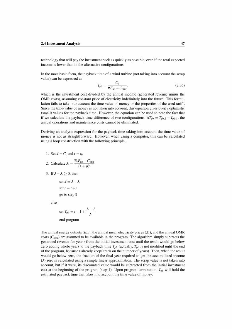
2.4 Investment Analysis 47
technology that will pay the investment back as quickly as possible, even if the total expectedincome is lower than in the alternative configurations.
In the most basic form, the payback time of a wind turbine (not taking into account the scrapvalue) can be expressed as
Tpb =Ci
πEao−Comr, (2.36)
which is the investment cost divided by the annual income (generated revenue minus theOMR costs), assuming constant price of electricity indefinitely into the future. This formu-lation fails to take into account the time-value of money or the properties of the used tariff.Since the time-value of money is not taken into account, this equation gives overly optimistic(small) values for the payback time. However, the equation can be used to note the fact thatif we calculate the payback time difference of two configurations, ∆Tpb = Tpb,2−Tpb,1, theannual operations and maintenance costs cannot be eliminated.
Deriving an analytic expression for the payback time taking into account the time value ofmoney is not as straightforward. However, when using a computer, this can be calculatedusing a loop construction with the following principle,
1. Set J =Ci and t = t0
2. Calculate Jt =π tEao−Comr
(1+ p)t
3. If J− Jt ≥ 0, then
set J = J− Jt
set t = t +1
go to step 2
else
set Tpb = t−1+Jt − J
Jt
end program
The annual energy outputs (Eao), the annual mean electricity prices (π t ), and the annual OMRcosts (Comr) are assumed to be available in the program. The algorithm simply subtracts thegenerated revenue for year t from the initial investment cost until the result would go belowzero adding whole years to the payback time Tpb (actually, Tpb is not modified until the endof the program, because t already keeps track on the number of years). Then, when the resultwould go below zero, the fraction of the final year required to get the accumulated income(J) zero is calculated using a simple linear approximation. The scrap value is not taken intoaccount, but if it were, its discounted value would be subtracted from the initial investmentcost at the beginning of the program (step 1). Upon program termination, Tpb will hold theestimated payback time that takes into account the time value of money.

48 Development of the Analysis Method
This variant of payback calculation was used in the analyses presented in this thesis. Unlessotherwise stated, the annual OMR costs were assumed zero and the scrap value was not takeninto account.
2.4.5 Implemented Tools
An Excel sheet was developed for the comparison of two alternative configurations. The sheetconsists of two parts. The purpose of the first one is to calculate the annual energy outputof a configuration, whereas the second part calculates the economic analysis. The outputof the AEO calculator (for two different configurations) is input to the economic analysis.Additionally, the tool calculates the partial derivatives of the AEO expression (Equations2.15 and 2.16).
In the AEO calculation sheet, for each configuration, the user specifies properties in threecategories: the wind, the turbine, and the electric drive train. The parameters are describedin Table 2.2. The turbine power coefficient Cp is calculated based on the nominal power,diameter, nominal wind speed, and air density. The power coefficient is assumed constantbetween the cut-in speed and the nominal speed. Above the nominal speed and below the cut-out speed, the turbine power is assumed constant. These assumptions idealize the behaviorof the turbine, which in reality, as demonstrated for instance by Kwon (2010), has statisticalvariation. When comparing different electric drive train configurations used with the sameturbine, the effect of these deviations from the ideal do not have as strong an effect on theoutcome as when comparing different turbines. If desired, they could, however, be accountedfor in the analysis.
The tool accepts Weibull distribution parameters to describe the wind conditions of the site.Furthermore, the user gives the desired number of bins and the lower and upper limits of thewind speed range that is divided into those bins. These must be selected by the user so thatno hours remain outside the bins; in practice, this means that the low limit is set to zero andthe high limit ”high enough”, somewhere around 30 m/s, for example. The tool calculatesthe durations of the bins based on the given Weibull parameters. The bins can also be createdor modified manually to facilitate input of time-series data or the creation of non-equal binwidths.
The total efficiency of the electric drive train (from mechanical input to electric output) isgiven as a table, where the efficiency is given as a function of wind speed. Thus, also theefficiency is given in the form of bins. These efficiency bins need not be the same as thewind speed frequency bins. Furthermore, the user can give an electric input power limit. Thisis meant to be used in situations where the electric drive train is undersized with respect tothe turbine, and the turbine output power must thus be limited. This kind of a situation isdiscussed in Case 2 in the next chapter. The efficiencies are obtained using a time domainsimulation tool, which calculates the output power of the system in various operating points.The tool is described in more detail in the next chapter.
In the economic analysis tool, the user specifies the parameters given in Table 2.3. Based

2.4 Investment Analysis 49
Table 2.2. Parameters that the user gives to the AEO calculation tool.Category Parameter Unit Typical data source / NotesTurbine Nominal power MW Turbine manufacturer
Diameter m ”Nominal speed r/min ”
Nominal wind speed m/s ”Cut-in wind speed m/s ”
Cut-out wind speed m/s ”Wind Density of air kg/m3 Meteorological data;
ρ = 1.225 kg/m3 commonly usedWeibull scale parameter m/s Wind atlases; measurementsWeibull shape parameter ”
Number of bins Set so that all time is allocated toWind speed range [m/s m/s] bins and the bin width is small enough
Electric Efficiency table As a function of wind speed;drive train obtaining from simulations discussed
in the next chapterMaximum power MW For limiting the turbine output
Table 2.3. Parameters that the user gives to the economic analysis tool.Parameter Unit Notes
Interest rate % Common to both configurationsAEO MWh For both conf’s, from the AEO calc. tool.
Turbine life years Estimated, often taken as 20 yearsInitial time index Time to commissioning (years) + 1
Tariff price eTariff duration yearsPost-tariff price e
on these, the income difference (Equation 2.23) between the configurations is calculated.The same interest rate is used for both configurations; other parameters can be set for eachconfiguration separately. The tariff system is currently limited to a fixed-price tariff with afixed duration. It would be relatively straightforward to make the tariff duration dependenton the performance of the plant (ending the tariff period after the first E MWh have beenproduced, for example); if the tool were to be used for a specific country, this would needto be done. The tool also calculates the payback time applying the method described inthe previous section. In the present version, OMR costs are taken as zero, which causesslightly underestimated payback times. Furthermore, the values of the partial derivatives ofthe income change expression (Equations 2.28 through 2.35) are calculated.

50 Development of the Analysis Method
2.5 Summary
This chapter discussed the fundamental physics of wind power production. An essentialfeature is that the power of wind is proportional to the cube of the velocity of the wind. Thisbrings forth the fact that the output power of a wind turbine decreases rather rapidly from thenominal, when the wind speed decreases from the nominal. Additionally, above the nominalwind speed, the power of a wind turbine is limited to the nominal value. Above the cut-outspeed or below the cut-in speed, the wind turbine is stopped. The description of statisticalwind properties was discussed. An estimate for the annual energy output (AEO) of a windturbine can be calculated, if the properties of the turbine (and the electric drive train) and thewind statistics are known. The calculation can be done by integrating over the distribution, orusing a discrete bin-based approach. It was shown that the methods give practically identicalresults provided that the bin width is sufficiently small, approximately 1 m/s or less. Thesensitivity of the AEO estimate to changes in the Weibull parameters was analyzed. A verybrief overview of the regulations concerning wind turbine design was given. The design(and possible optimization of it) needs to be done so that all relevant regulations are met.Simulations are often used to verify compliance with regulations.
In the latter part of the chapter, an economic analysis method was developed for comparingtwo alternative wind turbine configurations, with the focus on the properties of the electricdrive train. The idea of the method is to calculate the difference of the present value of thegenerated revenue over the life of the compared configurations. This comparison can answerat least two types of questions, namely 1) Should Configuration 1 or Configuration 2 beselected on economic grounds?, and 2) How much can a performance-improving modificationof a configuration cost in order to be feasible?, or, conversely, how much do we have to savewith a performance-degrading modification of a configuration in order for it to be feasible?,both being subject to a regulations-induced framework. In addition to calculating the incomechange, it was suggested that the calculation of the payback time could be used to supplementthe analysis to assess the risk associated with the change. An Excel sheet was created toautomate the analysis process.
Traditionally, economic analyses have been limited to rough feasible/not feasible analysesand determining the turbine power. After the feasibility of an installation is determined atthis level, the configuration of the electric drive train can be analyzed. The presented methodquantifies the economic performance of a change in the configuration, and gives the designerthe ability to express the economic feasibility of the change as a sum of money (and a paybacktime) instead of a mere efficiency change. The presented method requires information on thelosses in the electric drive train. This information can be supplied by a time domain simulator.Such a tool is discussed in detail in the next chapter.

51
Chapter 3
Simulations in the Wind TurbineTechnical and Economic Analysis
This chapter builds upon the material presented in the previous chapter, which introduced atechnical and economic analysis method for the assessment of the performance of a wind tur-bine electric power train and comparison of alternative configurations. In this chapter, first, theprinciples of loss modelling in a general-purpose transient simulation environment are stud-ied. The applicability of time domain simulations to be used in connection with the economicanalysis method presented in the previous chapter is tested with three (fictitious) examplecases: component selection, electric drive train nominal power selection (with fixed turbinesize), and high-level control principle selection in a modular low-voltage wind turbine drive.Finally, suggestions for further use cases are given.
3.1 Introduction
The previous chapter discussed the fundamentals of turning the kinetic energy of wind intoelectric energy and proposed a technical and economic analysis method to compare alter-native configurations. It was stated that the annual energy output of a wind turbine can becalculated, if the wind speed distribution, the power curve of the turbine, and the efficiency(as a function of wind speed or power) of the electric drive train are known. The first two –wind speed distribution and properties of the turbine – were discussed in the previous chapter.However, the efficiency of the electric drive train (which appears in the title of this book) wasnot yet covered.
This chapter consists of two rather distinct parts. In the first part, the components of a windturbine drive train are described, and modeling of their losses are discussed. In the secondpart, three different use cases of the technical and economic analysis utilizing the results of

52 Simulations in the Wind Turbine Technical and Economic Analysis
the simulations are presented. We will begin this chapter by describing the calculation ofelectrical losses in general.
3.2 Calculation of Powers and Losses
Efficiency is generally defined as the ratio of output power and input power,
η =Pout
Pin. (3.1)
For a wind power plant, the efficiency of the electric drive train is
ηe =Ppcc
Pmech, (3.2)
where Ppcc is the power at the point of common coupling (PCC, the point where the gen-erating plant is connected to the utility) and Pmech is the generator input mechanical power.Alternatively, using the loss term, this can be expressed as
ηe =Pmech−Ploss,e
Pmech, (3.3)
where Ploss,e represents the total losses of the electric drive train. Thus, for the determinationof the efficiency at various operating points, a method to calculate the electric power or thelosses at different points of the drive train is required.
Instantaneous electric power is, as is well known, defined as the product of a voltage accrossa circuit element and the current flowing through that element,
p(t) = u(t)i(t), (3.4)
where the power p, the voltage u, and the current i are generally functions of time t. If thevoltage and current are sine waves with a constant frequency, the power can be calculatedusing phasors with the equation
p = ui∗, (3.5)
where the asterisk (*) denotes the complex conjugate. In the commonly used three-phasesystem with a 120-degree phase shift between the phase voltages, the power is
p(t) = u10(t)i1(t)+u20(t)i2(t)+u30(t)i3(t), (3.6)
where ux0 denotes the phase-to-neutral voltage of phase x. In the space vector form (peakvalue scaling) the instantaneous power can be expressed in various forms,
p(t) =32
Reuuuiii∗= 32
uuu · iii = 32|uuu||iii|cosϕ. (3.7)

3.2 Calculation of Powers and Losses 53
In practical electric drives, especially those based on power electronic converters, the volt-age and current waveforms are never perfectly sinusoidal; aside from the fundamental fre-quency they contain to various degree harmonics, interharmonics, subharmonics, and a zero-frequency (DC) component. Furthermore, the phase sequence can be positive (L1 leading L2leading L3), negative (L1 leading L3 leading L2), or zero (L1, L2, L3 in the same phase).Space vectors can represent all positive and negative sequence components. However, thezero sequence components of a voltage or current do not show in the corresponding spacevector.
Measurements always attainable from a time-domain simulation are the phase currents andphase-to-phase voltages. Phase-to-neutral voltages are not directly available, if there is noneutral wire. A virtual star point using three identical resistors can be created, but, again,for the zero sequence voltages, the phase to virtual star point voltages would be zero. If thecommon-mode current does not exist, the instantaneous three-phase power can be obtainedusing the Aron method, which requires two phase-to-phase voltage measurements, two cur-rent measurements, and assumes that the sum of the currents equals zero Tumanski (2006).Depending on the choices made in the derivation of the expression, different forms will beobtained. One option is, with time indices omitted for all quantities,
p = u31i3−u12i2, (3.8)
where p is the instantaneous power, u31 is the voltage measured between phases 3 (positive)and 1 (negative), u12 is the voltage between phases 1 and 2, and i2 and i3 are the phase currentsof phases 2 and 3, respectively.
If the three-phase system under study does not have a neutral wire, then there is no galvanicpath for the zero sequence current to flow1. If there is a neutral wire connected to the compo-nent under study, Equation 3.6 gives also the zero sequence power. Between these two cases,there is a third alternative, in which there is a neutral wire or ground connected to some com-ponents of the system, but not all. This kind of situation is depicted in Figure 3.1, wherethe generator star point and the transformer (generator side) star point are grounded. In thatsystem, the zero sequence currents may flow through the device even if there apparently is noneutral conductor.
If, instead of power, we calculate the power loss over a component, even the contribution ofthe zero sequence can be detected. The component has two three-phase terminals, A and B.The phase-to-phase voltages and phase currents are measured at both terminals. Additionally,the voltages between the terminals A and B (voltages over the component) are measured.With these measurements, the loss can be expressed (Appendix A) as
ploss =(uAB3−uA31)iA1 +(uAB3−uAB1−uA31)iB1
+(uAB3 +uA23)iA2 +(uAB3−uAB2 +uA23)iB2
+uAB3iA3, (3.9)
where iAn, n = 1,2,3, are the phase currents at the A terminal, iBn, n = 1,2, are the phasecurrents at the B terminal, uA31 is the voltage between phases 3 and 1 and uA23 the voltage
1In a real system, the current may flow as a capacitive displacement current through various stray capacitances.No such mechanisms were modeled in the simulation models created for this study, however.

54 Simulations in the Wind Turbine Technical and Economic Analysis
Fig. 3.1. Measuring losses in the component under study. There can be losses caused by zero-sequencecurrents even though the component itself does not have a neutral wire. The path for the current isformed because the star points of the generator and the transformer are grounded.
between the phases 2 and 3 at the A terminal, and uABn, n = 1,2,3, are the voltages overthe component (A to B). The only assumption in the calculation (aside from assuming noneutral wire) is that the sum of the currents entering and exiting the component is zero (i.e.,the component does not have a third terminal).
To conclude, three different methods for power and loss measurement were used,
1. Equation 3.6. Power calculation. Neutral wire (reference potential) must be available.Includes the contribution of all positive and negative sequence components as well asthe zero sequence.
2. Equation 3.8. Power calculation. No neutral wire. The Aron method. Includes the con-tribution of all positive and negative sequence components but not the zero sequencecomponent.
3. Equation 3.9. Loss calculation. No neutral wire. Includes the contribution of all posi-tive and negative sequence components as well as the zero sequence.
3.3 Modeling the Losses in the Simulation
The design of a wind turbine is a very multi-disciplined task. Electrical aspects of the processinclude the design of the generator and other drive train components, as well as the controlalgorithms, the network connection, and fault tolerance. Simulations are a very useful toolanalyzing many of the subproblems associated. Accurate simulation of all loss mechanisms ina subsystem would require a detailed and comprehensive model of the subsystem. Generally,however, when implementing a loss model for a simulation, the goal is to obtain a model thatcan take into account those mechanisms which are relevant for the analyzed case. Therefore,

3.3 Modeling the Losses in the Simulation 55
the requirements of the simulator and the simulation model will differ from case to case.Modeling of high-frequency phenomena might, for example, require tuning equivalent circuitparameters based on measurements. The required bandwidth could be estimated based on apower spectrum analysis, for example.
Many papers have been published about using simulation software in the study of the be-havior of the wind energy conversion system in transient situations, including network dis-turbances. Simulations that aim at studying the dynamics of the power system containingwind generation often use a time step significantly longer than the period of the frequenciesoccurring in voltage-source inverter drives and, consequently, ignore the details of how theelectric drive operates. For example, Slootweg et al. (2003) have presented a general modelutilizable to represent both DFIG-based and full power converter (with PM machine) basedvariable speed turbines. In their simulations, a time step of 10 ms is used, and the generatoris modeled as a torque source. Akhmatov et al. (2000) present a thorough analysis of theinteraction between the power network and a wind turbine equipped with a constant speedinduction generator. Their study concentrates on the modeling of the turbine itself, includingthe mechanical resonances of the turbine rotor. In another article largely by the same authors(Akhmatov et al., 2003), the modeling of a wind farm of 80 such wind turbines (2 MW each)is discussed. In both papers, the electric drive train consists of the generator only, and thegenerator is modeled basically as a speed-torque curve. The effects of different generatorparameter (resistances, inductances) selections on the stable operating area of the generatorare analyzed, but the efficiency of the electric drive train is not considered.
Furthermore, a lot of scientific contribution has been made recently in the field of fault ride-through studies. Seman et al. (2006) compared three different approaches to voltage dip ridethrough capability of a DFIG-based turbine. They found out that simplifying the turbinemodel to a constant speed, constant torque representation did not have a significant effect onthe results. Furthermore, they note that a FEM (finite element method) model of the generatorcan be used in conjunction with the transient simulator to model high-frequency phenomenasuch as skin effect. This did not have a significant effect on the transient study results in thiscase. In the efficiency analysis, skin and proximity effect as well as saturation might have tobe taken into account in some cases. This cannot be done using the standard two-axis modelof an electric machine. Modified two-axis models with parallel current paths in the statorwinding have been developed to take into account skin effect (see e.g. (Thiringer, 1996)),and these could be used as an alternative to FEM modeling. Generally, it can be concludedthat simulators and models utilized in FRT studies are more suitable to the efficiency analysisthan those applied in power system dynamics studies.
There is a vast array of commercial simulation tools available that can be utilized to simulatethe electric behavior of a wind turbine. Some, such as PSS/E and PSCAD, are more suitablefor simulating the power network and its interactions with the generating plant, whereas oth-ers, such as Saber or PSpice, are focused on simulating electronics (Akhmatov et al., 2000,Lund et al., 2005, Iov et al., 2002). MATLAB/Simulink, on the other hand, is a general pur-pose simulation platform for simulating dynamic systems. It can be used stand-alone, or inconnection with other software. Uski et al. (2004) have demonstrated the use of Simulink inconnection with PSCAD and ADAMS (a mechanics simulator). Iov et al. (2004) presented a

56 Simulations in the Wind Turbine Technical and Economic Analysis
wind power simulation platform with MATLAB/Simulink as the basic modelling tool that canbe connected to other simulation software (Saber, HAWC, DIgSILENT). In 2008, a projectwas started at Lappeenranta University of Technology in co-operation with The Switch Ltd.to develop a MATLAB/Simulink-based tool for the simulation of wind power electrical sys-tems. The tool, called SwitchTool, includes models for transformers, filters, bridges, ma-chines and the like as well as the required generator and network control blocks (Luukkoet al., 2009b). The models utilize standard Simulink blocks and blocks from the SimPower-Systems extension. SwitchTool is capable of simulating both fixed-speed and variable-speedsystems, and aims to be user friendly and extensible. The tool can be used for instance todevelop control algorithms and analyze the behavior of the generating plant in the case of anetwork disturbance (protection, regulations compliance).
As a part of SwitchTool, a dedicated tool for efficiency analysis was developed. The toolsimulates a SwitchTool model in specified operating points and calculates the losses and theexported power. The calculations are defined by the user. Likewise, the operating points(in the form of wind speeds) are specified by the user. Figure 3.2 illustrates the parts of theanalysis system. The procedure for comparing two alternative configurations could be thefollowing:
1. Create models for the compared configurations. SwitchTool blocks can be used (theyutilize both plain Simulink blocks and blocks from the SimPowerSystems extension).Also, other blocks could be used. Ideally, the models (or one of them) already existand are used for other purposes.
2. Select powers and losses to be recorded. Add required power/loss measurement blocks(found in the SwitchTool library). Create expressions for the required calculations(calculation of the total efficiency); input to SwitchToolEff as an XML file.
3. Select operating points; input to SwitchToolEff as an XML file.4. Allow SwitchToolEff to run the simulations for the selected operating points and cal-
culate the efficiencies. Repeat for all compared configurations.5. Import efficiencies to the economic analysis Excel sheet (discussed in the previous
chapter). Select the wind data. Calculate analysis.
A power/loss calculation block was implemented in SwitchTool. This block can be used tocalculate and export the instantaneous power at a node (using Equation 3.8) or the loss overa component (Equation 3.9) with a PUI_loss block connected to both terminals of the com-ponent. The average values of losses are calculated by SwitchToolEff after the simulation isfinished. Since the total efficiency is calculated from the generator input mechanical powerto the electrical power exported to the network, also the mechanical power needs to be cal-culated. Since the generator load torque and the rotation speed are known, the mechanicalpower can be calculated using the equation
P = ωT, (3.10)
where P is the power, ω is the angular frequency of the rotation (ω = 2πn/60, where n is therotation speed in RPM), and T is the torque. An example of models used with SwitchToolEffcan be found later in this chapter, for example in Figure 3.7.
The value of simulations in the technical and economic analysis depends on the loss mech-

3.3 Modeling the Losses in the Simulation 57
Fig. 3.2. Simulation and analysis software as a block diagram.
anisms that show in the simulations. The following sections detail the loss mechanisms in awind power drive based on a permanent magnet generator and a full-power converter, whichis the type of the wind power drive in all of the simulation examples presented in this chapter.An example of the main components of the electric power train of a such system is presentedin Figure 3.3. In the figure, the wind turbine feeds mechanical power to the PM generator,which is connected to the frequency converter through a generator filter. The converter is con-nected to the power network through the transformer, and there is a network filter betweenthe transformer and the converter. The applicability of the utilized simulator to the analysis ofeach loss mechanism is discussed in connection with the discussion of the loss mechanism.
Fig. 3.3. Main components of a wind power drive train based on a PM generator and a full powerconverter. The generator and network filters are shown here as LCL filters, but they could be of anytype, or there might be no generator filter at all. Switchgear and protective devices not shown.

58 Simulations in the Wind Turbine Technical and Economic Analysis
3.3.1 Generator
Losses in an electrical machine generally consist of copper losses, iron losses, mechanicallosses, and additional losses (Pyrhönen et al., 2008). Copper losses (or, Joule losses) areresistive losses caused by current flowing in the windings of the machine. For a three-phasemachine,
PCu = 3I2R, (3.11)
where R is the resistance of one winding. In principle, copper losses are straightforward tomodel by including a stator resistance in the generator model. However, the resistance isgenerally frequency-dependent; the resistance increases with increasing frequency as a resultof skin effect and proximity effect. Since the generator is supplied by a frequency converter,the generator voltage contains harmonics of the fundamental frequency component. Using aconstant stator resistance in the generator model, copper losses caused by both the fundamen-tal and the harmonics will be captured. However, the frequency-dependent phenomena willbe ignored. The rotation speed of a gearless wind power turbine is relatively small (approx.10–30 RPM). Therefore, the supply fundamental frequency can also be low (although it mayalso be higher, over 50 Hz). It can be assumed, however, that the constant resistor modelis sufficient in many cases. Copper losses are the dominant loss mechanism in such slowlyrotating PM generators (see, e.g., simulation results by Polinder et al. (2006) and Tan et al.(2005)).
The stator resistance is also a function of temperature and thus dependent on the operatingpoint of the generator and the ambient temperature. The temperature of the winding can beestimated, if the power dissipation is known and there is a thermal model of the generator.Since the power dissipation (the losses) is a function of temperature, the process is iterative.No thermal modelling was included in the simulator, and thus the effect of temperature wasignored. The effect of temperature could, however, be taken into account either by manuallyadjusting the resistance (e.g. for different ambient temperatures) or including a thermal modelin the model with the power loss as an input and stator resistance as an output.
Iron losses (core losses) are usually the second most important loss mechanism in a PMgenerator. Iron losses consist of two parts: hysteresis losses (∝ f ) and eddy current losses(∝ f 2) (Hanselman, 2003). To represent the core losses of a PM machine, a core loss resis-tor Rc is added to the machine model and equations. Wijenayake and Schmidt (1997), forexample, present a modified de−qe equivalent model for a PM machine starting from a per-phase equivalent circuit with the core loss resistor in parallel with the internal voltage source.Model parameters (magnetizing inductances, stator resistance, voltage and current sources)are modified to include the effect of the core losses. For example, the Simulink model of a PMgenerator included in the Wind Turbine Blockset developed by Aalborg University and RISØNational Laboratory includes an optional iron loss resistor (Iov et al., 2004). The resistorvalue is a function of the mechanical rotation speed of the generator thus taking into accountthe core loss variation as a function of electrical frequency. However, the effect of harmonicsis more difficult to take into account in this model. For more accurate representation of theiron losses, a FEM model can be used (Mi et al., 2003), and the model can be combined witha time domain simulator (Seman, 2006). Iron losses and saturation may have to be taken intoaccount when the compared systems differ in terms of for example harmonic content in the

3.3 Modeling the Losses in the Simulation 59
generator terminal voltage. Notwithstanding the difficulties in iron loss modeling, it can stillbe said that it is more straightforward to do using the simulation-based loss calculation thanthe analytical one. However, in the case examples presented in this chapter, it was assumedthat the iron losses in the compared configurations were negligible in comparison with copperlosses, and they were not included in the models.
Mechanical losses and additional losses comprise losses for instance from friction (∝ ωmech),generator cooling and electromagnetic losses other than resistive and iron losses (Pyrhönenet al., 2008). Due to their diversity, they are difficult to estimate and model. However,their effect is often insignificant compared with copper and iron losses. For example, theIEC 60034-2:1996 standard (IEC, 1996) defined additional losses to be equal to 0.5 % of theestimated input power at rated load.
The models used in the simulation included only copper loss resistance, and thus no other lossmechanisms were taken into account. Therefore, in the simulations, it was assumed that theiron losses (as well as friction losses and additional losses) are insignificant compared withthe copper losses, and that the compared generators do not differ significantly in terms of ironloss characteristics. These might be justifiable assumptions, especially if the generators areslowly rotating and the voltage waveforms (in terms of harmonic content) in their terminalsare relatively similar. If the simulator is used for comparing generators with different iron losscharacteristics, then the generator model has to be modified to include an iron loss resistancein the machine equations. For accurate modeling, again, measurements of actual componentsin different operating points would be needed.
3.3.2 Filters
Loss mechanisms in filter inductors are rather similar to those in the generator; losses occurin the conductors (copper loss) and the core (hysteresis loss, eddy current loss). The inductorscan be modeled using some of the standard Foster or Cauer equivalent circuits. Figure 3.4presents a series-Foster equivalent circuit of an inductor. The circuit consists of the DCresistance and N elements in series, each of the elements consisting of an ideal inductor and anideal resistor in parallel. The idea of the model can be qualitatively understood by consideringthe circuit at different frequencies. With a DC input, current flows through the DC resistanceand through the series-connected ideal inductors (which represent a zero impedance at DC).The loss in this resistance corresponds to zero-frequency (no skin effect) copper loss. As theinput frequency is increased, more and more current is diverted to the resistances in parallelwith the inductances thus increasing the losses. The number of segments in the model mustbe selected by the user. The model parameters are most accurately defined by measurements.When based on a loss measurement, this kind of a model models the losses of the inductor as afunction of frequency, and the loss modeled contains contribution of all frequency-dependentloss mechanisms (copper loss increase caused by skin effect and iron losses).
This equivalent circuit was used in all the simulations presented in this chapter. As no realfilter components or data were available, a very simple version of the circuit was used. Thecircuit consisted of the DC resistance with one RL element in series. The value of the in-

60 Simulations in the Wind Turbine Technical and Economic Analysis
Fig. 3.4. Foster series equivalent circuit with N elements for an inductor.
ductance was taken as the nominal inductance of the inductor, and the parallel resistance wasselected such that it is approximately equal to the reactance (XL = ωL) of the inductor at afrequency of tens of kilohertz to a hundred kilohertz.
In addition to the inductors, also the filter capacitors are lossy components. A commonlyused simple model of a capacitor is the series connection of an ideal capacitor (equal to thenominal capacitance), an ideal resistor (the equivalent series resistance, ESR), and an idealinductor (the equivalent series inductance, ESL), shown in Figure 3.5. In this work, thecapacitors were modeled simply as an ideal capacitance with the ESR in series (ESL equal to0).
Fig. 3.5. RLC equivalent circuit of a capacitor.
The voltage waveforms in the terminals of a voltage source converter contain, in addition tothe fundamental frequency, various higher-frequency components extending up to the mega-hertz range (Skibinski et al., 1999). The simulation-based approach, although not entirelytrivial, is thus nonetheless more straightforward than forming an analytical expressions forthe losses in a filter.
3.3.3 Power Electronic Converter
The converter consists of a generator-side converter and a network-side converter, which areconnected back-to-back by the DC link. The DC link can be a voltage source (capacitor) or acurrent source (inductor). Here, it is assumed that the DC link is of the voltage source type,but nothing prevents the simulation of current source inverters. The converter is assumed tobe a four-quadrant one with both the generator and network converters implemented usingIGBT (insulated gate bipolar transistor) switches.

3.3 Modeling the Losses in the Simulation 61
Table 3.1. Switching energies as a function of load current direction (IL positive towards the load) andgate command change (1: upper leg conducting; 0: lower leg conducting).
0 → 1 1→ 0IL > 0 Eon EoffIL < 0 Eoff Eon
IGBT Bridges. An IGBT-based power electronic switch contains an IGBT transistor andan antiparallel diode. The losses of the switch can be divided into two parts: conductionlosses and switching losses. Conduction losses can be modelled with an on-state resistanceand voltage drop over the device. Modeling the switching losses is more difficult with thesimulation environment and models used in the present work. The IGBT models may enablea simulation using non-ideal switching waveforms. However, switching the transistor or thediode on or off is a very fast phenomenon (in the order of hundreds of ns or less) comparedwith the simulation time step used (ca. 1 µs). Therefore, the switching losses cannot directlybe contained in the simulation results, but the switching times must be set to zero and theswitching losses have to be obtained by other means.
The switching losses can be obtained by simulating the modeled system over a short periodwith a small time step (separately from the main simulation, solely to obtain the switchinglosses). Because of the limitations of the particular simulation environment, this could notbe done. Switching losses can also be estimated based on the information found in the datasheet of the device, which typically contains a graph of switching energies as a function ofdevice (collector) current for one or more device voltages. Switchings can be grouped intotwo cases:
1. The IGBT turns on and the antiparallel diode turns off. Switching energy Eon.2. The IGBT turns off and the antiparallel diode turns on. Switching energy Eoff.
The diode turn-on energy is typically insignificant compared with the other energies, andcan therefore be assumed zero (Kouro et al., 2008). Therefore, switching energies can beexpressed as (Kouro et al., 2008)
Eon = EIGBT,on +Ediode,off (3.12)Eoff = EIGBT,off (3.13)
When a gate command changes, the associated loss (Eon or Eoff) depends on the directionof the change (0→ 1, 1→ 0, 1 denoting ”upper leg switch on, lower leg switch off” and 0correspondingly ”upper leg switch off, lower leg switch on”) and the direction of the loadcurrent in the phase. If the current flowing towards the load is denoted positive, the switchingenergies have values presented in Table 3.1 (based on the work by Kouro et al. (2008)).
In the simulator, a Simulink block was implemented to record switching energies based onthe logic presented in Table 3.1 and the switching energy values taken from the data sheet(as a function of collector current). The energies are converted to switching loss power by

62 Simulations in the Wind Turbine Technical and Economic Analysis
the efficiency analysis tool. Switching waveform measurements can be used to obtain a moreaccurate estimate of the switching energies.
DC Link Circuit. The DC link capacitor can be modeled using the same models as inthe case of filter capacitors. In the simulations, a simple ideal capacitance with an equivalentseries resistance (ESR) was used. Similarly, if there is a DC filter inductor in the circuit, it canbe modeled using some of the standard inductor models (Foster/Cauer). In the simulations,no DC link inductor was used.
3.3.4 Transformer
Transformer loss mechanisms are generally similar to those found in inductors and generators(for transformer modeling, see e.g. (de León and Semlyen, 1994)), that is, copper losses andcore losses. In the simulations, the symmetrical transformer model provided by SimPower-Systems was used. Copper losses were modeled by the winding resistances, and the otherloss mechanisms were ignored.
3.4 Example Cases
This section presents three example cases of the usages of the proposed method. All casesare fictitious (not based on any existing or planned installation); their intended meaning isto illustrate some of the possible uses of the method. The first case involves two alternativecomponent selections, the second case two alternative electric drive trains, and the third casetwo alternative high-level control principles of a modular converter.
Component prices used in the calculations aim to be in a realistic order of magnitude, butit should be stressed that the results of the cases themselves are not the point of the section.Rather, the point is to test and illustrate the usage of the method in different kinds of situa-tions. All simulations presented were run with a discretization sample time 1 µs and variablestep Dormand-Prince ODE45 solver. In addition to the three cases, other possible use casesare suggested.
3.4.1 Case 1: Component Selection
This case tests the usage of the simulation-based approach in analyzing alternative componentselections. The case shows how the effect of different component selections shows in theeconomic analysis, that is, what is the monetary value of the component change. This valuecan be used by the designer to gauge the feasibility of the alternatives.

3.4 Example Cases 63
The drive under study is, as in all the other cases, based on a permanent magnet synchronousgenerator (PMSG) and a full power converter (block diagram presented in Figure 3.6). Thealternative components studied are two different IGBT modules. The modules differ in termsof nominal current, losses, and, presumably, price. The basic question that the designer wantsanswered is ”how much more can the component with lower losses cost in order to be morefeasible?” The analysis is calculated for three different wind conditions, described later.
Fig. 3.6. Block diagram of the simulated system.
A simulation model was created for Simulink utilizing the SwitchTool models described byLuukko et al. (2009b). A screenshot of the model with explanatory labels is presented inFigure 3.7. Blocks indicated by blue arrows are specific to the loss calculation. The cal-culated quantities are the mechanical power, the generator electric output power, converterlosses (switching losses and others), network filter losses, transformer losses, and power atthe point of network connection. In addition to adding the loss calculation blocks, no othermodifications of the basic simulation model were required for the efficiency analysis. Simi-lar models were created also for the other cases. The model parameters are discussed in thefollowing section.
Drive Train Parameters
The turbine specifications are based on the 1.5 MW direct drive configuration (generatorstator outside diameter 5.3 m) analyzed by Bywaters et al. (2004). Some of the parametersand characteristics of the drive components and other simulation blocks are presented inTable 3.2. As can be seen, the only differing parts are the network and generator converters.Switching losses were modeled as described in the previous chapter. Switching loss valuesfor different device currents (at junction temperature T = 125 C) were tabulated from thedatasheets (Dynex Semiconductor, a,b).

64 Simulations in the Wind Turbine Technical and Economic Analysis
Fig. 3.7. Screenshot of the Simulink model used. Blue arrows denote blocks specific to the loss calcula-tion.
Table 3.2. Parameter values and other properties of the compared configurations, Case 1. In con-nection with the switching losses, the nominal current Inom is the nominal current of the module(1600 A/1800 A). Transformer parameters are non-reduced.
Configuration 1 Configuration 2(”Basic”) (”Oversized”)
Turbine nominal power, MW 1.55nominal wind speed, m/s 12cut-in wind speed, m/s 3cut-out wind speed, m/s 25nom. rotation speed, RPM 19.6diameter, m 70.5
Generator nominal apparent power, MVA 1.7nominal power, MW 1.55nom. voltage (line-to-line), V 690nominal frequency, Hz 12.77pole pairs 39stator resistance, mΩ 15
Continued on the next page

3.4 Example Cases 65
Table 3.2 – ContinuedConfiguration 1 Configuration 2
(”Basic”) (”Oversized”)
Converter DC link capacitance, mF 57.6 57.6DC link capacitor ESR, mΩ 1.0 1.0switches IGBT + diode IGBT + diodeswitch module nom. current, A 1600 1800switching freq., network/gen., kHz 3.6/3.0 3.6/3.0IGBT forward voltage, V 2.6 2.6diode forward voltage, V 2.1 2.6on-state resistance, mΩ 0.27 0.09IGBT switch-on loss at Inom, mJ 150 175IGBT switch-off loss at Inom, mJ 350 390diode switch-on loss at Inom, mJ 0 0diode switch-off loss at Inom, mJ 160 195
Network type LCLfilter network-side (NS) inductance, µH 62.8
converter-side (CS) inductance, µH 105.2capacitance, mF 0.53total DC resistance, mΩ 4NS inductor parallel resistance, Ω 40GS inductor parallel resistance, Ω 66
Transformer nominal power, kVA 2000nominal frequency, Hz 50nominal voltage (HV/LV), V 20 000/690vector group Dyn11HV resistance, Ω 0.02HV inductance, mH 0.132LV resistance, mΩ 2.0LV inductance, µH 7.0magnetization resistance, Ω 220 000magnetization inductance, H 100
Network nominal line-to-line voltage, kV 20nominal frequency, Hz 503-phase short circuit power, MW 100reactance/resistance ratio 6

66 Simulations in the Wind Turbine Technical and Economic Analysis
Table 3.3. Weibull parameters of the wind speed distributions used in the simulation. Data for Bogskärfrom (Tammelin, 1991), others from (Finnish Wind Atlas 2009).
Location c k Height, m NotesBogskär 9.1 2.41 50 Open sea.Enontekiö 9.2 2.2 100 Inland. Hilly terrain with no trees.Lappeenranta 7.4 2.6 100 Inland, < 1 km from lake Saimaa.
Table 3.4. Bins and their durations used in the simulation.Start End Midpoint Duration Notes
Bogskär Enontekiö Lappeenranta0 3 1.5 584 714 799 Stopped3 5 4 1259 1302 18555 7 6 1768 1681 24207 9 8 1841 1685 20279 11 10 1503 1387 1129
11 12 11.5 556 534 27012 25 18.5 1249 1455 261 Lim. to nom. power25 30 27.5 0 1 0 Stopped
Wind Speed Distribution
The analysis was calculated with three wind speed distribution representing different typesof locations in Finland. The Weibull coefficients for the locations are given in Table 3.3.The first location is based on the data given by Tammelin (1991) for the Bogskär weatherstation situated in the open sea approximately 60 km SSE from the city of Mariehamn in theÅland Islands off the south-western coast of mainland Finland. The parameters are takenat the mast heigth of 50 meters. The second location is Enontekiö in the extreme north-west of Finland. The landscape is generally hilly and open, trees being stunted or missingaltogether. The mast height is taken as 100 m. The data were taken from the new Finnishwind atlas published online in November 2009 (Finnish Wind Atlas 2009). The third locationis Lappeenranta in the south-east of Finland roughly 100 km from the southern coast. Thewind conditions in the location are affected by the proximity of the largest lake in Finland,lake Saimaa. The coefficients were taken from the Finnish Wind Atlas 2009. Graphs of thewind speed distributions are presented in Appendix B.
The distributions were divided into bins of non-equal widths by an Excel program as depictedin Table 3.4. Bin midpoints were used as the wind speed value for the corresponding bin inthe simulation. Thus, the simulation was run for wind speeds 4, 6, 8, 10, 11.5 and 18.5 m/s.Since the power is limited to nominal, 18.5 m/s corresponds to the nominal wind speed,12 m/s.

3.4 Example Cases 67
Table 3.5. Total efficiencies of the drives in the simulated operating points.Efficiency
vw [m/s] Conf. 1 Conf. 24 0.783 0.8056 0.926 0.9278 0.943 0.943
10 0.926 0.92711.5 0.908 0.909
12-25 0.901 0.901
Table 3.6. AEO for the compared configurations in different wind conditions with the correspondingAEO differences.
Location EAO,1, MWh EAO,2, MWh ∆EAO, MWhBogskär 4885 4891 6
Enontekiö 4970 4976 6Lappeenranta 3021 3026 5
Simulation Results
The total efficiencies of the drives in the simulated operating points are given in Table 3.5.The annual energy outputs (EAO) of the compared configurations and their differences (∆EAO)were calculated using the wind speed distributions discussed above. The AEO calculationwas performed using the bin method (using the bin midpoint wind speed as the wind speedvalue and assuming the efficiency constant over the whole bin) with bin width 0.5 m/s. Theresults are given in Table 3.6.
Economic Analysis
The alternative configurations were compared applying methods presented in section 2.4.The question was: ”How much more can Configuration 2 cost than Configuration 1 in orderto be more feasible?” To answer this question, the difference of the generated revenue wascalculated using Equation 2.24 with ∆Ci = 0 and ∆E taken from Table 3.6. Payback timedifferences were not calculated in this case. In the calculation, the values presented in Table3.7 were used. The results are presented in Table 3.8.
With these values, it was obtained that the maximum investment cost increase is approxi-mately 3 000–4 000 e, which corresponds to 0.2–0.4 % of the investment cost. The invest-ment costs were taken directly from the report by Bywaters et al. (2004). The estimate isfrom the year 2004, the dollar-to-euro conversion has been made with simply replacing theunit (i.e., exchange rate 1.000), the prices do not include the price of the transformer or thenetwork filter, and the estimate is the manufacturing cost, not the sales price. All these factorscontribute to uncertainty in the investment cost. However, it should be noted that in this kind

68 Simulations in the Wind Turbine Technical and Economic Analysis
Table 3.7. Parameters used in the economic analysis.Parameter Value Notes
Interest rate (p) 8 %Time to commissioning (t0) 2 years
Turbine life (T ) 20 yearsInvestment cost (ci) 1 092 800 e Bywaters et al. (2004) estimate
with 1 $=1 eTariff price of electricity (π1) 83.50 e/MWh Proposal for the Finnish tariff
Tariff duration (t1) 12 years Proposal for the Finnish tariffMarket price of electricity (π2) 30.00 e/MWh
Table 3.8. Results of the analysis: difference of the generated revenue when selecting Configuration 2instead of Configuration 1.
Wind Profile ∆J, e(%)Bogskär 4 022 (0.37)
Enontekiö 4 159 (0.38)Lappeenranta 3 168 (0.29)
of an analysis the investment cost itself is not needed; it was included here only for normaliz-ing the maximum investment cost increase. The investment costs are discussed in more detailin connection with the next case.
The sensivity of the results to changes in parameter values can be estimated with a sensitivityanalysis. To illustrate, the values of the partial derivatives of the income change expression(Equations 2.28–2.35) for the Bogskär case (Table 3.7, ∆EAO = 6 MWh) are presented inTable 3.9. The values in the table give an estimate of the change in the income difference ∆J(Equation (2.27)) when a parameter is changed (change in e per amount in parentheses).
It can be seen that the result is very sensitive to changes in the annual energy output difference.The sensitivity of the AEO to changes in the wind conditions were analyzed previously, see
Table 3.9. Sensitivity analysis of the income difference ∆J (Equation (2.27)). Localized to the pointdefined by the parameter values in Table 3.7 and ∆EAO = 6 MWh.
Changed Parameter Change in ∆J, eInterest rate (p) -612 (%-unit)−1
AEO difference (∆EAO) 808 (MWh)−1
Turbine life (T ) 63 (year)−1
Time to commissioning (t0) -236 (year)−1
Inv. cost difference (∆ci) -1 (e)−1
Tariff price (π1) 51 (e)−1
Tariff duration (t1) 166 (year)−1
Market price of electricity (π2) 21 (e)−1

3.4 Example Cases 69
Table 3.10. Sensitivity of the AEO difference to changes in Weibull parameter values.Wind Profile ∂∆Eao
∂c , MWh/(ms−1) ∂∆Eao∂k , MWh
Bogskär 0.8 -0.3Enontekiö 0.7 -0.2
Lappeenranta 0.4 -0.4
Table 3.11. Absolute maximum errors in the Weibull parameters.Wind Profile c, m/s k AEO
Bogskär 9.1±0.9 2.41±0.24 6±0.8Enontekiö 9.2±0.9 2.2±0.22 6±0.7
Lappeenranta 7.4±0.7 2.6±0.26 5±0.4
Equations 2.15 and 2.16. Now that we are analyzing the sensitivity of the AEO differenceinstead of the plain AEO, these equations can be rewritten as
∂∆Eao
∂c= T
kc
N−1
∑i=0
[(vi,l
c
)kexp(−(vi,l
c
)k)−(vi,h
c
)kexp(−(vi,h
c
)k)]
∆Pe,i, (3.14)
∂∆Eao
∂k= T
kc
N−1
∑i=0
[(vi,h
c
)kexp(−(vi,h
c
)k)
ln(vi,h
c
)−
(vi,l
c
)kexp(−(vi,l
c
)k)
ln(vi,h
c
)]∆Pe,i, (3.15)
where ∆Pe,i is the electrical power difference between the configurations in bin i. The valuesof the partial derivatives were calculated for each of the wind profiles. Table 3.10 presentsthe results.
Let us assume that both of the Weibull parameters have an error of 10 %. Furthermore, let usfor now assume that the electric power (mechanical power times the total efficiency) exportedto the network is correct for all bins. This gives the absolute Weibull parameter values givenin Table 3.11. Table 3.11 also lists the AEO errors with these assumptions.
If the two compared cases share similar wind conditions (as in this case), then the AEOdifference can be written as
∆Eao =N−1
∑i=0
∆η(vi)P(vi)Ti, (3.16)
where ∆η(vi) are the efficiency differences for different wind speeds (obtained from simu-lations). Assuming that the mechanical power P is known exactly and keeping the Weibullparameters and thus the bin durations Ti constant, it can be seen (applying the triangle in-equation, |x+y| ≤ |x|+ |y|) that the error in ∆Eao is less than or equal to the sum of the errorsin each bin,
|∆(∆Eao)| ≤N−1
∑i=0|∆(∆η(vi))P(vi)Ti|. (3.17)

70 Simulations in the Wind Turbine Technical and Economic Analysis
Table 3.12. Annual energy output differences for the three locations, with tolerances.Wind Profile AEO Max. error, %
Bogskär 6±1.8 30Enontekiö 6±1.8 30
Lappeenranta 5±1.3 26
Thus, for example, if each of the efficiency differences can be assumed to be known with anaccuracy of 20 %, then the maximum error in the AEO difference caused by this is 20 % aswell. Continuing the previous example, the lower and upper limits of the AEO differencepresented in Table 3.11 can be expanded to values given in Table 3.12. The assumptionswere that the maximum error in the Weibull parameters is 10 % and the maximum error inthe efficiency differences was 20 %. Furthermore, the two errors were calculated independentof each other (assuming the other variable known).
It can be concluded that the AEO differences can be assumed to be known (in this case) withan accuracy of approximately ±2 MWh or better. This would create a maximum error ofapproximately 1 000–2 000 e in the difference of the present values of the generated incomeof the compared configurations, which corresponds to roughly 20–50 %.
Looking at Table 3.9, we can see that also the interest rate p has a relatively large influenceon the present value of the income difference, ∆J. Increasing interest rate will decrease ∆J.Therefore, selecting a high interest rate will favor Configuration 1. Changes of approximately2–4 %-unit would be required to create a similar effect on ∆J as the uncertainty of the AEOdifference calculated above.
With this kind of a tariff, the tariff price and duration are known at the investment moment.The market price of electricity after the tariff period does not have a significant effect on theanalysis result. The investment cost difference can be expected to be reasonably well knownto the turbine manufacturer. The time to commissioning is also known with an accuracy ofone to two years, and the turbine life does not have a significant impact on the result.
It can thus be concluded that the two significant contributors to the uncertainty in the analysisresult are (in this case) the uncertainty in the AEO difference and the future interest (and infla-tion) rate. Uncertainty in the AEO difference is caused both by uncertainty in the future windconditions and the uncertainty in the efficiency differences. The former can never be totallyeliminated, since there is annual variation in the wind conditions. Accurate measurementdata are needed to minimize that effect. The latter can, in principle, be eliminated very wellwith good simulation models. The models used in this example case are far from perfect, andthat they must be, since there are no real configurations which they would attempt to model.With actual components and configurations, more accurate models could be constructed.
Finally, it could noted that although the income differences obtained in this example aresmall, less than 5 000 e, the cumulative effect might be significant. In 2008, the new in-stalled wind power capacity was 27 GW (Global Wind Energy Council). This correspondsto approximately 18 000 wind turbines like the one discussed in the example. So, although

3.4 Example Cases 71
the maximum cost increase in this example was less than 5 000 e, the great number of newinstallations scales this to 90 million e globally.
Conclusion
This case demonstrated the utilization of the simulation-based approach to the output energycalculation in the technical and economic analysis of a wind turbine electric drive train. Twoalternative IGBT module selections were analyzed in three different wind conditions. Anestimate was obtained for the monetary value of selecting an oversized module instead ofthe nominally sized one. This value depends on the wind conditions, and can be used bythe designer to gauge the feasibility of component selections. Loss calculation blocks wereadded to simulation models utilized in the study of control algorithms and fault ride-through;no other modifications were made.
A benefit of the simulation-based approach over analytic calculation of losses is the fact thatvoltage waveforms in the simulation resemble, depending on the quality of the models, wave-forms occuring in real systems. Therefore, loss contribution from all frequencies could beincluded in the calculation. However, models applied in the case did not include mechanismsto take into account some frequency-dependent phenomena, such as skin effect in the genera-tor windings. This kind of phenomena would nonetheless be more straightforward to includein the calculation using the simulation-based approach than analytic calculation of losses.Simulation model development is required if more accurate loss figures are needed.
Another significant benefit of the simulation-based approach is the fact that the effect of thecontrol principle of the generator can be taken into account. In this example, the controlmethod applied was the standard id = 0 control. If there were alternative implementations ofthe generator control, the different control blocks could be the components under study.
It can be concluded that the simulation-based approach is very useful in this kind of a study.The electric drive train must be considered as a whole, where changes in one component mayresult in changes in losses of other components. It is more straightforward to take this kindof interactions into account by using the simulation-based approach than it is using analyticcalculation of losses. A simulation of this kind can be used to refine component selectionsafter the basic topology and size of the wind energy conversion system have been decidedupon.
3.4.2 Case 2: Electric Drive Train Sizing
In the second case, the simulation-based approach is tested in a site matching-type problem.Site matching of wind energy conversion systems has been traditionally done ignoring theeffect of the electric drive train, as was discussed in the previous chapter. This case exampleaims to test if the inclusion of the electric drive train could have an effect on the analysis.

72 Simulations in the Wind Turbine Technical and Economic Analysis
The example problem is partial site matching in the sense that the size and other propertiesof the turbine are fixed. The nominal power of the turbine is 2 MW. However, the company(wind power manufacturer or integrator) has at its disposal full power converters with ratingsof 1.5 MW and 3 MW, and the generator power can be selected to match the power of theturbine or the converter. Thus, two different configurations can be offered to the customer:
• Configuration 1 (undersized): 2-MW turbine, 1.5-MW generator, 1.5-MW full powerconverter
• Configuration 2 (oversized): 2-MW turbine, 2-MW generator, 3-MW full power con-verter
With configuration 1, the power output of the 2-MW turbine must be limited to 1.5 MWby blade pitch control, whereas with configuration 2, the full nominal output power of theturbine can be fed to the converter. Figure 3.8 illustrates the output power of a 2-MW turbineas a function of wind speed without power limitation (solid line) and with power limited to1.5 MW (dashed line).
0 5 10 15 20 25 300
0.5
1
1.5
2
x 106
Wind Speed [m/s]
Tur
bine
Out
put P
ower
[W
]
Fig. 3.8. Theoretical power output of a 2-MW turbine (solid line), limited to 1.5 MW (dashed line).
The effect of the power limitation on the mean annual power (and annual energy output) ofthe turbine cannot be determined from Figure 3.8 alone, because the wind speed distributiondetermines the duration of hours when the power output is limited. The effect of the limi-tation can be graphically gauged by weighing the turbine power output curve with the windspeed frequency distribution function and plotting the resulting curve. The weighed curvecorresponds to the integrand (Pw(v)p(v)) in Equation 2.6. Figure 3.9 presents an example ofsuch a curve. The wind speed Weibull distribution parameters are k = 2.41 and c = 9.10 m/s(the ones used for Bogskär in the previous Case).
The area below each curve corresponds to the annual average power output of the configura-tion. This multiplied by one year (8760 hours) yields the average annual energy output. The

3.4 Example Cases 73
0 5 10 15 20 25 300
2
4
6
8
10
12x 10
4
Wind Speed [m/s]
Con
trib
utio
n to
Mea
n P
ower
[W/(
ms−
1 )]
Fig. 3.9. Contribution of different wind speeds to the mean annual output (Pw(v)p(v) in Equation 2.6)with the turbine power not limited (solid line) and limited to 1.5 MW (dashed line). Calculated withWeibull parameters k = 2.41 and c = 9.10.

74 Simulations in the Wind Turbine Technical and Economic Analysis
area above the dashed line and below the solid line corresponds thus to the lost productiondue to power limitation. Using numerical integration (trapezoidal rule), the AEO difference inthis case can be calculated to be 767 MWh, which corresponds to a 11-% decrease comparedwith the non-limited case.
This analysis does not take into account the efficiency of the electric drive train, but mightbe a good starting point. Some of the income change equations (e.g. Equation 2.27) can beused to calculate the relative feasibility of the two configurations. However, in reality, theconfigurations might not be identical in the area below the power limitation. To take this intoaccount, we will again utilize simulations.
Drive Train
Both configurations have a low-voltage (LV) permanent magnet (PM) generator supplied bya full-power four-quadrant frequency converter. The LV converter is connected to the 20-kVnetwork using a transformer. A network filter is connected between the converter and thetransformer. In the models, the filter is an LCL filter. Alternatively, a CL filter could be used,effectively using the transformer as an additional filter inductance. Some parameter valuesand other properties of the subsystem simulation models for the two alternative configurationsare presented in Table 3.13. It can be noted that only those parts that are not part of the electricpower train (the turbine and the network) are completely identical in both cases.
The two drive train configurations were modeled in Simulink/SwitchTool. Simulations wererun in different operating points, and the total efficiencies of the configurations were calcu-lated. The results are presented in Table 3.14.
Drive Train Cost Estimates
Prices of wind turbines and their components and subsystems are generally trade secrets. Thisis not a problem, however, because the aim of this book is not to present absolute feasibilitycalculations of any particular turbine or turbine type but, rather, to present an analysis methodthat can be used by those who can better estimate the costs. However, cost estimates of somegrade are required to be able to illustrate the usage of the method. Bywaters et al. (2004)compared various wind turbine configurations in terms of their costs. Their estimates for twodirect-drive permanent magnet configurations are presented in Table 3.15. Bywaters et al.(2004) discuss two 1.5-MW DD configurations, the one in the table is the variant with adiameter of 5.3 m.
The ”normalized sales price” (dollars/kilowatt) can be used to estimate the price of corre-sponding systems or components of different power ratings. Alternatively, the nominal torqueof the machine could be used as the basis of the normalization. The electrical torque can be

3.4 Example Cases 75
Table 3.13. Parameter values and other properties of the compared configurations. Transformer pa-rameters are non-reduced.
Configuration 1 Configuration 2(undersized) (oversized)
Turbine nominal power, MW 2.0nominal wind speed, m/s 12cut-in wind speed, m/s 3cut-out wind speed, m/s 25nom. rotation speed, RPM 15.3diameter, m 88
Generator nominal power, MW 1.5 2.0nom. voltage (line-to-line), V 690 690nominal frequency, Hz 12.77 12.77pole pairs 50 50stator resistance, mΩ 0.015 0.0113
Converter switches IGBT + diode IGBT + diodeIGBT forward voltage, V 2.6 2.6diode forward voltage, V 2.1 2.1on-state resistance, mΩ 0.27 0.09DC link capacitance, mF 57.6 115.2DC link capacitor ESR, mΩ 1.0 0.5IGBT switch-on loss at Inom, mJ 150 200IGBT switch-off loss at Inom, mJ 350 600diode switch-on loss at Inom, mJ 0 0diode switch-off loss at Inom, mJ 160 260
Network type LCL LCLfilter network-side (NS) inductance, µH 41.9 31.4
converter-side (CS) inductance, µH 70.1 52.6capacitance, mF 0.795 1.06total DC resistance, mΩ 1.33 1NS inductor parallel resistance, Ω 26 20GS inductor parallel resistance, Ω 44 33
Transformer nominal power, kVA 2000 2500nominal frequency, Hz 50 50nominal voltage (HV/LV), V 20 000/690 20 000/690vector group Dyn11 Dyn11HV resistance, Ω 0.8 0.6HV inductance, mH 0.132 0.106LV resistance, mΩ 0.7 0.55LV inductance, µH 7.0 5.6magnetization resistance, Ω 220 000 220 000magnetization inductance, H 100 100
Network nominal line-to-line voltage, kV 20nominal frequency, Hz 503-phase short circuit power, MW 100reactance/resistance ratio 6

76 Simulations in the Wind Turbine Technical and Economic Analysis
Table 3.14. Efficiencies of the compared configurations in different wind speed bins. The value isobtained by simulations with the bin midpoint as the wind speed.
Wind speed, Configuration 1 Configuration 2 Notesm/s (undersized) (oversized)0 – 3 0 0 Stopped3 – 5 0.827 0.8135 – 7 0.931 0.9327 – 9 0.940 0.9449 – 11 0.923 0.93711 – 12 0.911 0.92212 – 25 0.911 0.91525 – 0 0 Stopped
Table 3.15. Cost estimates for subsystems in direct drive permanent magnet (DDPM) wind turbines(Bywaters et al., 2004, Section 9.1).
1.5 MW 3 MWGenerator $185 000 (17.0 %) $420 000 (21.5 %)Nacelle $90 000 (8.3 %) $131 000 (6.7 %)Converter $121 000 (11.1 %) $180 000 (9.2 %)Turbine, cabling, tower etc. $612 000 (56.4 %) $1 041 000 (53.2 %)Freight, assembly $78 000 (7.2 %) $184 000 (9.4 %)Total $1 086 000 $1 956 000Projected sales price $1 257 000 $2 333 000Price/kilowatt $838 $778

3.4 Example Cases 77
Table 3.16. Normalized costs of the 1.5-MW and the 3-MW direct drive generators analyzed by Bywa-ters et al. (2004).
1.5 MW 3 MWEstimated cost $185 000 $420 000Nominal power 1.55 MW 3 MWNominal rotation speed 19.7 RPM 15.3 RPMNominal torque 751 kNm 1870 kNmCost/kW $119 $140Cost/kNm $246 $224
expressed as
TTT e =32
pψψψs× iiis, (3.18)
where TTT e is the electrical torque space vector, p is the number of pole pairs, ψψψm is thestator flux linkage space vector, and iiis is the stator current space vector (space vector lengthsnormalized to the peak value of the corresponding phase quantity sine wave). The electricalpower, on the other hand, is
Pe =32
uuus · iiis, (3.19)
where Pe is the electrical power, uuus is the stator voltage space vector, and iiis is the statorcurrent. As can be seen, both the power and the torque depend on the current and the voltage(in stationary state, uuus = jωψψψs). Additionally, the torque depends on the number of polepairs in the machine. The nominal synchronous rotation speed (in revolutions per minute) ofa generator is
nnom =60 fnom
p, (3.20)
where fnom is the nominal electrical frequency and p is the number of pole pairs. Thus, if nnomis to be decreased while keeping fnom constant, p must be increased. Consequently, slowlyrotating machines require generally more pole pairs than faster-rotating machines of the samenominal power rating. A higher number of pole pairs may also complicate the assembly andadd to the volume of the machine, thereby increasing costs. Therefore, the nominal torque isa more justified choice for the normalization than the nominal power. In practice, though, thecompared generators often do not differ significantly in terms of their nominal rotation speed,and the nominal power can be used as well. Prices normalized with the nominal power andthe nominal torque are given in Table 3.16. It can be seen that the cost-per-kW of the smallergenerator is lower than that of the larger generator. However, if the nominal torque is used asthe basis of the normalization, the situation is opposite.
The maximum torque of the undersized generator (nominal power 1.5 MW) is required at thewind speed where the power limitation becomes active, vw,lim. This wind speed is somewhatlower than the nominal wind speed vw,nom of the non-limited turbine. The wind speed androtation speed can be estimated with the following procedure. First, solving Equation 2.3 forthe wind speed vw, we obtain an expression for the required wind speed to produce power P,
vw =
(2P
ρACp
) 13. (3.21)

78 Simulations in the Wind Turbine Technical and Economic Analysis
Assuming the power coefficient Cp of the (non-limited) turbine constant in the interval[vw,lim,vw,nom], this can be simplified to
vw =
(P
Pnom
) 13
vw,nom. (3.22)
For limiting power P = Plim = 1.5 MW and nominal power Pnom = 2 MW, this yields vw,lim ≈10.9 m/s. To calculate the torque at this wind speed, the rotation speed of the turbine mustbe known. If the tip-speed-ratio λ (Equation 2.4) of the turbine is assumed constant over theinterval [vw,lim,vw,nom], the rotation speed nlim can be calculated from
nlim =vlim
vnomnnom. (3.23)
Setting vnom = 12 m/s, vlim = 10.9 m/s, and nnom = 15.3 RPM gives nlim = 13.9 RPM. Thus,the required generator torque is Tlim = 1.03 MNm. For the non-limited case, the maximumtorque is the nominal torque (Pnom = 2 MW and nnom = 15.3 RPM), which equals 1.25 MNm.Using the normalized generator cost $246/kNm, the prices of the generators are $253 000(1.5 MW) and $307 000 (2 MW). The 1.5-MW generator can be designed with 13.9 RPM asthe nominal rotation speed (and with overspeed capability up to at least 15.3 RPM), or thegenerator can be designed with the nominal speed of 15.3 RPM but with sufficient torquehandling capability at lower rotation speeds. The generator design affects the costs, but thisis beyond the scope of this book. In the analysis, we will use the above-calculated costs forthe generators.
The converter sizing is determined by the current handling capacity required, and this, in turn,is determined by the nominal apparent power of the generator. In this case, the two converteroptions were the 1.5-MW converter and the 3-MW converter. As cost estimates for these, thevalues in Table 3.15 were used.
The tower and foundation costs are affected by the weight of the nacelle. The main com-ponents of the nacelle are the turbine (which is the same in both configurations) and thegenerator. The power converter is assumed to be located on the ground. In this example case,the nacelle of the 2-MW turbine is presumably designed to support the weight of a 2-MWPM machine. In the undersized case (1.5-MW generator) the mechanical structure could bemade lighter, but in this example it is assumed that the generator/converter supplier cannotinfluence the nacelle or tower design and, thus, these costs are assumed equal in both cases.Furthermore, the prices of the turbine, cabling, tower, and nacelle were assumed to be linearlydependent on the nominal power of the turbine, and the values for these costs were taken fromthe 1.5-MW configuration costs in Table 3.15 by multiplying them with 2/1.5 = 4/3.
At this point it should be noted that the estimates presented by Bywaters et al. (2004) do notinclude the cost of the transformer. In his article concerning the design of a 1.5-MW DDwind generator (Zephyros Z72), Versteegh (2004) estimates the cost of the transformer to be2 % of the total cost of the turbine. Using the total cost of the undersized generator calculatedso far, it can be estimated that the transformer cost is approximately $30 000. Assuming theprice of the transformer to be linearly dependent on the rated apparent power, the price of theoversized transformer can then be estimated to be 2.5/2 · $30 000 ≈ $38 000. Furthermore,

3.4 Example Cases 79
Table 3.17. Cost estimates used in the Case.Configuration 1 Configuration 2
(undersized) (oversized)Generator 253 000 e 307 000 eConverter 121 000 e 180 000 eTurbine, tower, cabling; freight, assembly 1 040 000 e 1 040 000 eTransformer & network filter 60 000 e 76 000 eTotal cost 1 474 000 e 1 603 000 ePrice with 20 % profit margin 1 769 000 e 1 924 000 e
Table 3.18. Weibull parameters for the analysis. All parameters taken from the European Wind Atlas(Troen and Petersen (1989)) at the height of 100 m.
Location c k Roughness Notesclass
Ålborg, DK 9.8 2.24 1 Very flat terrainEindhoven, NL 7.9 2.42 2 Comparatively close to the seaHamburg, GER 7.8 2.43 2 Comparatively close to the sea
Saarbrücken, GER 7.0 2.27 2 Further inlandMunich, GER 5.8 1.45 2 Deep inland
the network filter costs are not included in the estimates presented by Bywaters et al. (2004).The costs can be estimated to be of the same order of magnitude as the transformer costs. Inthe analysis, we will assume that the network filter costs are identical to the correspondingtransformer costs.
Table 3.17 summarizes the estimated costs of the compared configurations. In the table,dollars have been converted to euros with $1 = 1 e. The values presented so far are the costsof the configurations; the sales prices will be higher. However, it is the sales price that thecustomer buying the turbine and producing the electricity needs to use in the analysis. In theanalysis, sales prices 20 % higher than the costs were used.
Economic Analysis
The analysis was made for various wind distributions acquired from wind atlases. The lo-cations and their corresponding Weibull parameters are listed in Table 3.18. Graphs of thedistributions used are presented in Appendix B. Ålborg in northern Jutland represents a com-paratively windy location. Eindhoven and Hamburg, both located less than 200 km from theNorth Sea, are rather similar in terms of wind conditions (noticeably less windy than Ålborg).Saarbrücken in Germany near the French border is about twice as far from the sea as Eind-hoven and somewhat less windy. Munich in Bavaria is located yet farther from the sea, andis clearly less windy than the other locations.

80 Simulations in the Wind Turbine Technical and Economic Analysis
Table 3.19. Parameters used in the economic analysis.Parameter Value Notes
Interest rate (p) 8 %Time to commissioning (t0) 2 years
Turbine life (T ) 20 yearsInvestment cost (ci) 1 769 000 e Configuration 1
1 924 000 e Configuration 2Tariff price of electricity (π1) 83.50 e/MWh
Tariff duration (t1) 12 yearsMarket price of electricity (π2) 30.00 e/MWh Assumed price after tariff period
Since the locations where the data have been acquired are in different countries, the locationswill also differ in terms of the remuneration for the produced energy. Germany, for example,uses a tariff-based system for on-shore wind power, in which the basic tariff is 50.20 e/MWhexcept during the first five years of operation, when an initial tariff of 92.00 e/MWh is used.This initial tariff is extended based on the performance of the wind power installation in com-parison with a reference installation. These values are valid for installations in operation be-fore 1 Jan 2010, and they decrease with 1 % per a year’s delay in commissioning (until 2015)(German Renewable Energy Act 2008, Article 1; §20,§29). Denmark, on the other hand, usesa premium-based system with a premium of 250 DKK/MWh (approximately 34 e/MWh 10Nov 2009) added to the electricity price during the first 22 000 full load hours of an on-shore wind turbine, that is, until 22 000 h ·Pnom/MW MWh of energy has been exported tothe network (Danish Renewable Energy Promotion Act 2008, Ch. 1, §36). In both Germanand Danish legislation, the duration of the tariff is thus dependent on the performance of theturbine.
To simplify the analysis and to eliminate the effect of different energy policies, the sameremuneration system is used with all wind speed distributions. The tariff selected is thesame as in the previous case, 83.50 e/MWh (12 years from commissioning). The economicparameters are shown in Table 3.19.
Results and Discussion
For each wind profile, the difference between the annual energy output of the two consideredconfigurations was calculated. Using this value and the estimated investment cost differenceand economic parameters given in Table 3.19, the difference in the present value of the in-come over the life of the turbine (∆J) was calculated. Furthermore, the difference betweenthe payback times of the two configurations was calculated as discussed in the previous case.The results are presented in Table 3.20.
In the first case (Ålborg), Configuration 2 (oversized converter) is clearly superior. The av-erage wind speed is so high that a significant amount of energy (1 GWh) per year will belost if an undersized converter and generator are selected. In the case of Eindhoven and Ham-

3.4 Example Cases 81
Table 3.20. Results of the economic analysis.Wind profile ∆AEO, MWh ∆J, e ∆Tpb, months Selected configuration
Ålborg 999 496 000 -4 Conf. 2Eindhoven 373 88 000 0 Conf. 2 (or Conf. 1)Hamburg 345 69 000 1 Either
Saarbrücken 211 -17 000 5 Conf. 1Munich 286 N/A N/A Neither
burg, both configurations are approximately equal in terms of economic performance. In bothcases, the present value of the generated electricity is slightly more when using Configuration2 than with Configuration 1. For Eindhoven, the payback times are equal; for Hamburg, thepayback time of Configuration is slightly less (1 month) than that of Configuration 2. Thereis no practical difference between the two configurations in terms of economic performance.For Saarbrücken, the present value of the generated electricity is practically equal for bothconfigurations (17 000 e more for Configuration 1). However, the payback time of Configu-ration 1 is five months less than that of Configuration 2, and it could be said that in this caseselecting Configuration 1 would be justified. For the final case, Munich, neither of the config-urations is economically feasible; the generated income for Configuration 1 is negative, andfor Configuration 2, barely above zero. The corresponding payback times are approximatelyequal to the life of the turbine.
As mentioned, site matching problems of this kind are usually calculated without taking intoaccount the effect of the electric drive train. The additional value obtained by the simulatorcan be gauged by calculating the corresponding analyses without the use of the simulator.Table 3.21 shows the economic analysis results for Case 2 calculated without the simulator,assuming that the efficiency of the electric drive train is constant 0.9 (independent of the op-erating point). Values obtained using the simulator are shown in parentheses (first presentedin Table 3.20). It can be seen that in none of the considered wind regimes, utilizing the sim-ulator instead of merely using the (guessed) constant efficiency has an effect on the outcomeof the analysis (i.e., the selection of the electric drive train configuration). Therefore, the useof a simulator with the kind of models presented here does not seem to bring much addi-tional information to analyzing the problem. However, with more detailed generator models,generator control and overloading analysis would be possible and might yield additional in-formation, which would be more complicated to obtain with analytic methods. Furthermore,a turbine aerodynamic model could be combined with the electrical model, enabling an anal-ysis of the dynamic performance of the drive for instance in gusts.
3.4.3 Case 3: Drive Train Control Evaluation
In the previous two cases, the selections involved two alternative hardware configurations.The third case attempts to evaluate the simulation-based approach in the selection of thecontrol methods and principles. Control development is very commonly carried out withthe help of a simulator, so it might be useful to obtain figures of the economic performance

82 Simulations in the Wind Turbine Technical and Economic Analysis
Table 3.21. Results of the economic analyses presented in the case with efficiency assumed constant0.9. The numbers in parentheses indicate results obtained using the simulator (Table 3.20).
Wind ∆AEO ∆J, e ∆Tpb, Selectedprofile MWh months configuration
Ålborg 952 (999) 466 000 (496 000) -5 (-4) Conf. 2Eindhoven 342 (373) 68 000 (88 000) 0 (0) Conf. 2 (or Conf. 1)Hamburg 315 (345) 50 000 (69 000) 1 (1) Either
Saarbrücken 189 (211) -32 000 (-17 000) 5 (5) Conf. 1Munich 269 (286) N/A N/A Neither
of the alternative control principles at the same time as obtaining figures of their technicalperformance. Furthermore, the effects created by selections in the control systems are oftensuch that they are difficult to analyze analytically. The combined implication of these twonotes is that this kind of an analysis can be expected to be one of the most suitable candidateusages of the simulation-based approach.
In this example, two high-level control principles of a modular low-voltage drive are com-pared. The nominal power of the wind turbine is a 4.5 MW, and the turbine drives a4.5-MW permanent magnet generator. The generator is connected to the network utilizingthree parallel-connected full-power IGBT-based converters each having a nominal power of1.5 MW. Parallel connection of power electronic converters, generally, is useful when highpower levels with low voltages are required. Other potential benefits over single-converterapproach include higher reliability and lower harmonic levels (see, for example, (Ye, 2000)).
In this example, the converters are connected to the network using a common transformer.Each converter has a dedicated network filter. There are no generator filters; the generator-side IGBT bridges are connected to each other and to the generator terminals. In real devices,power imbalance and circulating currents could arise resulting from differences in parame-ters, but in the simulation model, all IGBTs and other components can be made perfectlysimilar. On the other hand, the effects of component imbalances could be taken into accountin an equally straightforward way, and different parallelization schemes (e.g. separate statorsfor each converter, separate transformers or transformer secondaries for each converter) couldbe compared. A block diagram of the system is presented in Figure 3.10.
The network and the generator converter controllers give the same gate commands to all threenetwork and generator converters, respectively. In the example, converter control algorithmswere not compared. Instead, two higher-level control principles were compared:
• Alternative 1 (”All on”): All three frequency converters active whenever the turbineis rotating,
• Alternative 2 (”Staircase”): Different set of converters engaged at different power lev-els, such that converter 1 is always active (Pcut−in < P < Pcut−out), converter 2 is activewhen 1 MW < P < Pcut−in, and converter 3 is active when 2.5 MW < P < Pcut−out.
The capacity of the connected converters and the turbine output power as a function of wind

3.4 Example Cases 83
Fig. 3.10. Block diagram of the electric drive train of the system simulated in the case. One 4.5-MWPM generator is fed by three parallel-connected 1.5-MW full power converters.
speed is illustrated in Figure 3.11.
0 5 10 15 20 25 300
0.5
1
1.5
2
2.5
3
3.5
4
4.5
x 106
Wind Speed, m/s
Pow
er, W
Fig. 3.11. Enabled converters in Alternative 2: turbine output power (solid line) and connected con-verter capacity (dashed line) as a function of wind speed.
In this case, the hardware configurations for both alternatives are the same, and thus theinvestment cost difference ∆Ci is zero. However, the monetary value of the changing of thehigh-level control principle can be calculated using the same method as in the previous cases.This can, then, be weighed against the estimated cost of for instance changing the existingcontroller software. Table 3.22 lists the efficiencies obtained using the simulator.

84 Simulations in the Wind Turbine Technical and Economic Analysis
Table 3.22. Efficiencies of the alternative configurations (from simulations).Wind speed, Alternative 1 Alternative 2 Notes
m/s (all on) (staircase)0 – 3 0 0 Stopped3 – 5 0.716 0.8435 – 7 0.883 0.9327 – 9 0.935 0.945
9 – 11 0.940 0.93711 – 12 0.922 0.92312 – 25 0.918 0.917 Nominal
25 – 0 0 Stopped
Table 3.23. Increase in income (∆J) when the ”staircase” converter utilization scheme is used insteadof the ”all on” scheme.
Wind profile ∆AEO, MWh (%) ∆J, e
Ålborg 88 (0.5) 57 000Eindhoven 114 (1.1) 74 000Hamburg 116 (1.1) 75 000
Saarbrücken 124 (1.6) 81 000Munich 98 (1.5) 64 000
As could have been expected, the ”staircase” utilization yields higher efficiencies on lowloads. With higher loads, the efficiencies are equal (within variation caused by the simulator).The monetary value of implementing the ”staircase” converter utilization instead of the ”allon” utilization was calculated for the same wind data as in Case 2. The investment costs wereset equal for both configurations. Other economic parameters were taken from Table 3.19.Table 3.23 presents the results for different wind data (locations).
Utilization of the ”staircase” principle could thus have a significant effect on the generatedenergy and revenue. The simulation method could be used to find the optimal wind speeds(powers) for the converter combination changes. In this example, the two combinations weresimulated separately. However, adding parallel branches may increase the simulation timequite significantly. Therefore, a more feasible method could be to simulate only the efficiencyof one converter as a function of power, and then analytically divide the generator powerinto the active converters and calculate the combined efficiency. This method could thenbe used to find good combination selection criteria. However, with this method, possibleeffects of component imbalances could not be taken into account. These imbalances result incirculating currents, which increase losses.

3.4 Example Cases 85
Conclusion
In this case, the simulation-based approach was tested with a rather simple example of select-ing the converter utilization scheme in a full-power converter-based wind energy conversionsystem with three parallel-connected low-voltage converters. According to the simulations,one of the alternatives was clearly superior to the other. The simulation-based method is wellsuited for analyses of this kind, and it could be applied for instance to selection of gener-ator control algorithms and analysis of the losses caused by parameter deviations betweenparallel-connected converters. Since power levels in wind energy conversion systems areconstantly growing, a lot of research is focused on modularization, and several concepts havebeen proposed. Simulation-based technical and economic analysis can prove to be a veryuseful tool in comparing the alternative concepts.
3.4.4 Discussion
The three cases discussed above represented three different situations. The first one involvedtwo alternative component selections, in this case alternative IGBT modules. Clearly, inthis case, efficiency data for the considered components for different operating points is aprerequisite for the calculation of the technical and economic analysis. When designing acompletely new product, this kind of an analysis could be performed. In practice, however,the number of different components and modules is usually kept to a minimum, and, thus,the same components utilized in other models (or, for example, components from the samemanufacturer) are chosen for a new design. This limits the potential use of the method in thiskind of situations.
In the second case, the method was applied to the selection of the nominal power of theelectric drive train when the properties of the turbine were fixed (kind of a ”partial” site-matching problem). As seen in the Case, selection of the electric drive train may have asignificant effect on the economic performance of the installation (Table 3.20). However, inmany cases, the efficiency of the electric drive train has an insignificant effect on the outcomeof the analysis. Generator overloading analysis and including a turbine model as well as adynamic model of the wind conditions (including gusts) could provide additional informationnot obtainable using analytic calculation.
In the third Case, two high-level control principles were compared in the case of a turbinewith three converters operating in parallel. The goal was to compare two systems, which haddifferent criteria for selecting the combination of running converters. The simulator can beused to find a good (if not optimal) scheme. Since the hardware configuration is not changed,no direct investment cost difference is applicable to the analysis. However, for example,changing the required software may have a quantifiable cost.
Some cases that might be interesting to simulate are discussed in brief in the following para-graphs.

86 Simulations in the Wind Turbine Technical and Economic Analysis
Multi-level converters. Simulation and technical and economic analysis of a multi-level(e.g. three-level) converter vs. a traditional two-level converter in a wind turbine. This hasbeen previously discussed by e.g. Ikonen et al..
Modular converters. Discussed in Case 3. However, comparison of different topologies(see e.g. (Ye et al., 2000)) and comparison of multiple converters vs. multiple IGBT modules(see e.g. (Keller and Tadros, 1993)) could also be made.
Medium-voltage drives. As wind turbine sizes and power electronics ratings increase,medium-voltage (MV) turbines become feasible in more cases. Comparison of an MV andan LV (low-voltage) drive for a particular turbine and site could be made using the proposedmethod.
Control algorithms. Simulations can be used to estimate the performance of different con-trol algorithms. The results can be weighed with the wind speed distribution. Investment costdifference might be applicable in some cases (for example, speed sensor vs. no speed sensor).
Selection of components. Discussed in Case 1. Can be applied for instance to networkand generator filter selection (core material, parameters), cable sizing, design and sizing ofthe overvoltage protection (brake chopper, AC load), and others. Could also include, forexample, selection of the switching frequency.

87
Chapter 4
Conclusion and Discussion
This work discussed the feasibility of utilizing a time domain simulation used for the tech-nical analysis and development of a wind power drive train in the economic analysis andcomparison of different component and parameter selections. The benefits of the approachcompared with the analytical calculation of efficiencies were studied. The method was testedwith three example cases, and suggestions for further cases were given.
Chapter 2 introduced the required fundamental physics of wind power production. It waspointed out that the power of wind is proportional to the cube of the velocity of the wind,which brings forth the fact that the output power of a wind turbine decreases rather rapidlyfrom the nominal, when the wind speed decreases from the nominal. Chapter 2 also discussedthe description of statistical wind properties. It was noted that an estimate for the annualenergy output (AEO) of a wind turbine can be calculated, if the properties of the turbine(and the electric drive train) and the wind statistics are known. The calculation can be doneintegrating over the distribution, or using a discrete bin-based approach. It was shown foran example distribution that the methods give identical results provided that the bin widthis sufficiently small, approximately 1 m/s or less. The sensitivity of the AEO estimate tochanges in the Weibull parameters was analyzed. A very brief overview of the regulationsconcerning wind turbine design was given. The design (and possible optimization of it) needto be done so that all relevant regulations are met. Importantly, it was noted that simulationsare often used to verify compliance with regulations.
In the latter part of Chapter 2, an economic analysis method was developed. The method isutilizable in the comparison of two alternative wind turbine configurations, with the focuson the properties of the electric drive train. With the method, the difference in the presentvalue of the generated revenue over the life of the compared configurations is calculated. Thiscomparison can answer at least two types of questions, namely 1) Should Configuration 1 orConfiguration 2 be selected on economic grounds?, and 2) How much can a performance-improving modification of a configuration cost in order to be feasible?, or, conversely, Howmuch do we have to save with a performance-degrading modification of a configuration in

88 Conclusion and Discussion
order for it to be feasible?, both subject to the regulations-induced framework. In additionto calculating the income change, it was suggested that the calculation of the payback timecould be used to supplement the analysis.
Chapter 3 discussed the utilization of simulations to obtain the efficiency of the electric drivetrain required in the technical and economic analysis. The main loss mechanisms in a windenergy conversion system based on a permanent magnet (PM) machine and a full powerconverter were described, and their modeling in a time domain simulator was discussed.Based on the calculated efficiencies, the properties of the turbine, and the wind statistics,the annual energy outputs of the compared configurations can be calculated. An add-onto a simulation package specifically focused on the efficiency analysis was developed. Thefeasibility of the simulation-based approach was tested with three case examples representingdifferent use cases. The first one involved two alternative component selections (alternativeIGBT modules). In the second case, the method was applied to the selection of the nominalpower of the electric drive train when the properties of the turbine were fixed (a ”partial”site-matching problem). In the third case, two high-level control principles were comparedin the case of a turbine with three converters operating in parallel. Differences between thecompared configurations were clearly attainable from the simulations.
Cases to which the proposed method could be applicable include
1. Component selection
• Selection of alternative drive train components. For example, selection of differ-ent filter core materials.
• Benefits of the simulation-based approach over analytical loss calculation includethe possibility to take into account interactions between different components in amore straigthforward way. The result of the component change can be expressedas an income change, not merely an efficiency change. The feasibility of thechange can also be evaluated based on the payback time difference, which de-scribes the change in the risk associated with the component change. The effectof the change on the technical performance (e.g. fault ride-through) of the systemcan be checked using the same simulation.
• In practice, the designer may not be able to select components totally freely, butthere may nonetheless be alternatives.
• Simulations are an essential tool in this case, mainly because the system needs tobe considered as a whole (the total efficiency of the system is not generally theproduct of the efficiencies of the constituent components analyzed independentlyof the system).
• Example in Case 1 (selection of different IGBT modules).
2. Site matching
• Comparison of different wind energy conversion systems for a specific site.
• Traditionally carried out assuming a constant electrical efficiency (unity, or someother constant value). Simulations not needed in a rough feasible/not feasible

89
analysis. When optimizing the drive train configuration (components, parameters,control algorithms), however, simulations are again very useful or even required.
• If the choice is to be made between a number of configurations with fixed, verydifferent properties (different nominal powers, for example), the simulator maynot be needed.
• Illustrated in Case 2, where two different power classes for the frequency con-verter and generator were considered. In this case, the simulator did not providesignificant additional information compared with assuming the efficiency con-stant – except showing that assuming the efficiency constant in this case did notgenerate significant errors.
3. Siting (site selection)
• Comparison of different sites for a specific wind energy conversion system.• Somewhat similar to site matching. However, only one candidate system exists,
and, therefore, only one set of simulations is needed. The rough selection of thesite can be made without the simulator (as is traditionally done), but, again, if thedrive train parameters can be tuned, the simulator is required.
• Although site matching was the main focus of Case 2, also siting was demon-strated, since the economic performance of the two compared configurations wascalculated for multiple sites.
4. Control development
• Comparison of different control methods.• Illustrated at a high level in Case 3, where the staircase-like utilization curve of
the parallel-connected converters yielded superior performance, as could havebeen expected. Also, low-level control principles (generator converter control,network converter control) could be compared.
• Simulations widely applied to the design and analysis of control methods. Theperformance of the control is evaluated based on traditional control theory figures(such as step response) as well as based on the performance of the system in ab-normal situations (such as loss of network or voltage drop). The control methodscould also be evaluated based on their economic performance using the methodsdiscussed in this book. Simulations would be an essential tool in this kind of ananalysis.
5. Converter configuration
• Comparison of for example multilevel converters and two-level converters, ordifferent parallelization schemes.
• There are numerous schemes for the generator-converter combination in high-power wind energy conversion systems. Paralleled IGBT modules and paral-leled low-voltage converters enable an increase of current while still using a low-voltage generator. A medium-voltage generator, on the other hand, can be usedwith low-voltage converters in series or using a medium-voltage converter. Thestudy of these alternatives from a technical and economic point of view would bevery interesting.

90 Conclusion and Discussion
• Simulations would be a very useful tool, since interactions between the converterand the generator (as well as the possible filter) need to be taken into account.
The objective of this work was to assess the feasibility of utilizing a simulation-based ap-proach to the technical and economic analysis and comparison of alternative wind turbineconfigurations. It was shown that time domain simulations are a useful tool not only in theircurrent fields of application (analysis of technical performance), but also in the economicanalysis. The work can be used to analyze problems related to some of the areas listed above,or other types of wind-power-related problems. Successful utilization of the method requiressimulation models that accurately model the loss mechanisms of the specific components un-der consideration. These models could be verified using measurements of the actual config-urations. This work is intended to serve as a basis for further work. The eventual applicationof the method as well as the development and verification of the required models is left to thethose applying the method to analyze an actual problem.

Appendices


93
Appendix A
Loss Calculation over aThree-Phase Component
This appendix provides the derivation of an equation for the power loss over a non-balancedthree-phase two-terminal component with no neutral wire. The equation takes into accountthe contribution of both differential-mode and common-mode currents. Figure A.1 illustratesa ”black box” model of a two-terminal three-phase device and the measurable voltages. Ad-ditionally, all phase currents are measured.
Fig. A.1. Measured voltages in a ”black box” three-phase device.
Internally, the black box can be modeled using a three-phase T equivalent circuit, as shownin Figure A.2. Instantaneous currents and internal voltages of the model are also presented inthe Figure.

94 Loss Calculation over a Three-Phase Component
uA1
uA2
uA3
uA1
uA2
uA3
uB1
uB2
uB3
u1 u2 u3
iA1
iA2
iA3
iB1
iB2
iB3
uAB1, uAB2, uAB3
Fig. A.2. Model of the loss measurement from the terminals of a ”black box” three-phase system withtwo terminals. Phase-to-phase voltages, phase currents, and voltages over the component (per phase)measured.
The sum of the currents entering the device must be zero at all instants of time. Hence,
iA1 + iA2 + iA3 + iB1 + iB2 + iB3 = 0. (A.1)
The instantaneous power dissipation ploss (t) in the circuit is the sum of the power dissipationsin the component impedances. Using voltages and currents, this can be written as
ploss =uA1iA1 +uB1iB1 +u1 (iA1 + iB1)
+uA2iA2 +uB2iB2 +u2 (iA2 + iB2)
+uA3iA3 +uB3iB3 +u2 (iA3 + iB3) . (A.2)
All voltages in the equation are unknown. However, either voltages uAx or uBx (where x =1,2,3) can be eliminated, since uABx = uAx−uBx. We choose to eliminate uBx by substitutinguBx = uAx− uABx in Equation A.2. Performing the substitution and rearranging the termsyields
ploss =(uA1 +u1) iA1 +(uA1−uAB1 +u1) iB1
+(uA2 +u2) iA2 +(uA2−uAB2 +u2) iB2
+(uA3 +u3) iA3 +(uA3−uAB3 +u3) iB3. (A.3)
One of the current terms can be eliminated using Equation A.1. We choose to substituteiB3 =−iA1− iA2− iA3− iB1− iB2. This gives
ploss =(uA1 +u1−uA3 +uAB3 +u3) iA1 +(uA1−uAB1 +u1−uA3 +uAB3 +u3) iB1
+(uA2 +u2−uA3 +uAB3 +u3) iA2 +(uA2−uAB2 +u2−uA3 +uAB3 +u3) iB2
+uAB3iA3. (A.4)

95
The expression can be simplified using Kirchhoff’s voltage law for selected loops. The loopequations are
−uA31 =uA1 +u1−u3−uA3 (A.5)uA23 =uA2 +u2−u3−uA3. (A.6)
Substituting these into Equation A.4 gives the expression
ploss =(uAB3−uA31)iA1 +(uAB3−uAB1−uA31)iB1
+(uAB3 +uA23)iA2 +(uAB3−uAB2 +uA23)iB2
+uAB3iA3, (A.7)
which is Equation 3.9.
This form contains only quantities that can be measured outside the ”black box”. Otherselections in the derivation of the equation would have resulted in a different but equivalentform.

96 Loss Calculation over a Three-Phase Component

97
Appendix B
Wind Distribution Graphs
This appendix presents the wind speed distribution graphs for the locations used in the exam-ple cases.
5 10 15 200
0.02
0.04
0.06
0.08
0.1
0.12Bogskar: c = 9.1, k = 2.41
Wind Speed, m/s
Fig. B.1. Bogskär, Finland.

98 Wind Distribution Graphs
5 10 15 200
0.02
0.04
0.06
0.08
0.1Enontekio: c = 9.2, k = 2.20
Wind Speed, m/s
Fig. B.2. Enontekiö, Finland.
5 10 15 200
0.02
0.04
0.06
0.08
0.1
0.12
0.14
0.16Lappeenranta: c = 7.4, k = 2.60
Wind Speed, m/s
Fig. B.3. Lappeenranta, Finland.

99
5 10 15 200
0.02
0.04
0.06
0.08
0.1Alborg, DK: c = 9.8, k = 2.24
Wind Speed, m/s
Fig. B.4. Ålborg, Denmark.
5 10 15 200
0.02
0.04
0.06
0.08
0.1
0.12
0.14Eindhoven, NL: c = 7.9, k = 2.42
Wind Speed, m/s
Fig. B.5. The Netherlands.

100 Wind Distribution Graphs
5 10 15 200
0.02
0.04
0.06
0.08
0.1
0.12
0.14Hamburg, GER: c = 7.8, k = 2.43
Wind Speed, m/s
Fig. B.6. Hamburg, Germany.
5 10 15 200
0.02
0.04
0.06
0.08
0.1
0.12
0.14Saarbrucken, GER: c = 7.0, k = 2.27
Wind Speed, m/s
Fig. B.7. Saarbrücken, Germany.

101
5 10 15 200
0.02
0.04
0.06
0.08
0.1
0.12
0.14Munich, GER: c = 5.8, k = 1.45
Wind Speed, m/s
Fig. B.8. Munich, Germany.

102 Wind Distribution Graphs

REFERENCES 103
References
Affärsverket Svenska Kraftnät (2005), “Affärsverket Svenska Kraftnäts föreskrifter ochallmänna råd om driftsäkerhetsteknisk utformning av produktionsanläggningar,” On-line, http://www.svk.se/Global/07_Tekniska_krav/Pdf/Foreskrifter/SvKFS2005_2.pdf, ac-cessed Mar 3 2009.
Aggarwal, S.K., Saini, L.M., and Kumar, A. (2009), “Electricity price forecasting in dereg-ulated markets: A review and evaluation,” Electrical Power & Energy Systems, vol. 31,no. 1, pp. 13–22.
Ahmed Shata, A.S. and Hanitsch, R. (2008), “Electricity generation and wind potential as-sessment at Hurghada, Egypt,” Renewable Energy, vol. 33, no. 1, pp. 141–148.
Akhmatov, V., Knudsen, H., and Nielsen, A.H. (2000), “Advanced simulation of windmills inthe electric power supply,” International Journal of Electrical Power and Energy Systems,vol. 22, no. 6, pp. 421–434.
Akhmatov, V., Knudsen, H., Nielsen, A.H., Pedersen, J.K., and Poulsen, N.K. (2003), “Mod-elling and transient stability of large wind farms,” International Journal of ElectricalPower and Energy Systems, vol. 25, no. 2, pp. 123–144.
de Alegría, I.M., Andreu, J., Martín, J.L., Ibañez, P., Villate, J.L., and Camblong, H. (2007),“Connection requirements for wind farms: A survey on technical requirements and regu-lation,” Renewable and Sustainable Energy Reviews, vol. 11, no. 8, pp. 1858–1872.
Archer, C.L. and Jacobson, M.Z. (2005), “Evaluation of global wind power,” Journal ofGeophysical Research, , no. 110.
Aspliden, C.I., Elliot, D.L., and Wendell, L.L. (1986), Resource Assessment Methods, Sitingand Performance Evaluation, pp. 321–376, New Jersey: World Scientific.
Baroudi, J.A., Dinavahi, V., and Knight, A.M. (2007), “A review of power converter topolo-gies for wind generators,” Renewable Energy, vol. 32, no. 14, pp. 2369–2385.
Burton, T., Sharpe, D., Jenkins, N., and Bossanyi, E. (2001), Wind Energy Handbook, JohnWiley & Sons Ltd.
Bywaters, G., John, V., Lynch, J., Mattila, P., Norton, G., Stowell, J., Salata, M., Labath, O.,Chertok, A., and Hablanian, D. (2004), “Northern power systems WindPACT drive train

104 REFERENCES
alternative design study report,” National Renewable Energy Laboratory (NREL) Subcon-tractor Report NREL/SR-500-35524.
Carlin, P.W., Laxson, A.S., and Muljadi, E.B. (2001), “The history and state of the art ofvariable-speed wind turbine technology,” Tech. Rep. NREL/TP-500-28607, National Re-newable Energy Laboratory (NREL).
Carlin, P.W. (1997), “Analytical expressions for maximum wind turbine average power ina Rayleigh wind regime,” in Proceedings of the 16th American Society of MechanicalEngineers Wind Energy Symposium, Reno, Nevada, USA.
Celik, A.N. (2003), “Energy output estimation for small-scale wind power generators usingWeibull-representative wind data,” Journal of Wind Engineering and Industrial Aerody-namics, vol. 91, no. 5, pp. 693–707.
Coelingh, J.P., van Wijk, A.J.M., and Holtslag, A.A.M. (1996), “Analysis of wind speed ob-servations over the North Sea,” Journal of Wind Engineering and Industrial Aerodynamics,vol. 61, no. 1, pp. 51–69.
Couture, T. and Gagnon, Y. (2010), “An analysis of feed-in tariff remuneration models: Im-plications for renewable energy investment,” Energy Policy, vol. 38, no. 2, pp. 955–965.
Danish Renewable Energy Promotion Act 2008 (2008), “Lov om fremme af vedvarende en-ergi,” Online, http//www.retsinformation.dk, accessed 10 Nov 2009.
Dynex Semiconductor (a), “DIM1600FSM12-A single switch IGBT module datasheet,” On-line, www.dynexsemi.com, accessed Oct 1 2009.
Dynex Semiconductor (b), “DIM1800ESM12-A single switch IGBT module datasheet,” On-line, www.dynexsemi.com, accessed Oct 1 2009.
E.ON Netz GmbH (2006), “Grid code, high and extra high voltage,” Online, http://www.eon-netz.com, accessed Mar 3 2009.
Finnish Wind Atlas 2009 (2009), “Suomen tuuliatlas (Finnish wind atlas),” Online,http://www.tuuliatlas.fi, accessed 11 Dec 2009.
Fleten, S.E., Maribu, K.M., and Wangensteen, I. (2007), “Optimal investment strategies indecentralized renewable power generation under uncertainty,” Energy, vol. 32, no. 5, pp.803–815.
Fouquet, D. and Johansson, T.B. (2008), “European renewable energy policy at crossroads –focus on electricity support mechanisms,” Energy Policy, vol. 36, no. 11, pp. 4079–4092.
German Renewable Energy Act 2008 (2008), “Gesetz zur Neuregelung des Rechts derErneuerbaren Energien im Strombereich und zur Änderung damit zusammenhängenderVorschriften,” Bundesgesetzblatt, Jahrgang 2008, Teil I, Nr. 49.
Global Wind Energy Council (), “Global wind 2008 report,” Online,http://www.gwec.net/fileadmin/documents/Global%20Wind%202008%20Report.pdf,accessed Oct 20 2009.

REFERENCES 105
Gorban’, A.N., Gorlov, A.M., and Silantyev, V.M. (2001), “Limits of the turbine efficiencyfor free fluid flow,” Journal of Energy Resources Technology, vol. 123, pp. 311–317.
Grauers, A. (1996), “Design of direct-driven permanent-magnet generators for wind tur-bines,” Doctoral thesis, Chalmers tekniska högskola, Gothenburg, Sweden.
Hanselman, D. (2003), Brushless Permanent Magnet Motor Design, Cranston, Rhode Island:The Writers’ Collective, second edn.
Hansen, A.D. and Hansen, L.H. (2006), “Wind turbine concept market penetration over 10years 1995−2004,” Wind Energy, vol. 10, no. 1, pp. 81–97.
Hansen, L.H., Helle, L., Blaabjerg, F., Ritchie, E., Munk-Nielsen, S., Bindner, H., Sørensen,P., and Bak-Jensen, B. (2001), “Conceptual survey of generators and power electronics forwind turbines,” Tech. Rep. Risø-R-1205(EN), Risø National Laboratory, Roskilde, Den-mark.
Hoogwijk, M., de Vries, B., and Turkenburg, K. (2004), “Assessment of the global and re-gional geographical, technical and economic potential of onshore wind energy,” EnergyEconomics, vol. 26, no. 5, pp. 889–919.
van der Hoven, I. (1956), “Power spectrum of horizontal wind speed in the frequency rangefrom 0.0007 to 900 cycles per hour,” Journal of Meteorology, vol. 14, no. 2, pp. 160–164.
Ibenholt, K. (2002), “Explaining learning curves for wind power,” Energy Policy, vol. 30,no. 13, pp. 1181–1189.
IEC (1996), IEC 60034-2: Rotating electrical machines — Part 2: Methods for determininglosses and efficiency of rotating electrical machinery from tests (excluding machines fortraction vehicles), Geneva, Switzerland.
IEC (2002), IEC 61000-4-7: Electromagnetic Compatibility (EMC) — Part 4-7: Testing andmeasurement techniques — General guide on harmonics and interharmonics measure-ments and instrumentation, for power supply systems and equipment connected thereto,Geneva, Switzerland: International electrotechnical commission, 2nd edn.
IEC (2005), IEC 61400-12-1: Wind turbines — Part 12-1: Power performance measurementsof electricity producing wind turbines, Geneva, Switzerland: International electrotechnicalcommission, 1.0 edn.
IEC (2008), IEC 61400-21: Wind turbines — Part 21: Measurement and assessment of powerquality characteristics of grid connected wind turbines, Geneva, Switzerland, 2.0 edn.
Ikonen, M., Laakkonen, O., and Kettunen, M. (), “Two-level andthree-level converter comparison in wind power application,” Online,http://www.elkraft.ntnu.no/smola2005/Topics/15.pdf, accessed Dec 2 2009.
Iov, F., Blaabjerg, F., Chen, Z., Hansen, A.D., and Sørensen, P. (2002), “A new simula-tion platform to model, optimize and design wind turbines,” in Proceedings of the IEEE2002 28th Annual Conference of the Industrial Electronics Society (IECON 2002), Sevilla,Spain, Nov 5–8, 2002.

106 REFERENCES
Iov, F., Hansen, A.D., Sørensen, P., and Blaabjerg, F. (2004), “Wind turbine blockset in Mat-lab/Simulink,” Tech. rep., Institute of Energy Technology, Aalborg University, Denmark.
Johnson, G.L. (2001), Wind Energy Systems, public domain, electronic edn.
Jowder, F.A.L. (2009), “Wind power analysis and site matching of wind turbine generators inKingdom of Bahrain,” Applied Energy, vol. 86, no. 4, pp. 538–545.
Junginger, M., Faaij, A., and Turkenburg, W.C. (2005), “Global experience curves for windfarms,” Energy Policy, vol. 33, no. 2, pp. 133–150.
Justus, C.G., Hargraves, W.R., Mikhail, A., and Graber, D. (1978), “Methods for estimatingwind speed frequency distributions,” Journal of Applied Meteorology, vol. 17, no. 3, pp.350–353.
Kaldellis, J.K. and Gavras, T.J. (2000), “The economic viability of commercial wind plantsin Greece – a complete sensitivity analysis,” Energy Policy, vol. 28, no. 8, pp. 509–517.
Keller, C. and Tadros, Y. (1993), “Are paralleled IGBT modules or paralleled IGBT invertersthe better choice?” in Proceedings of the Fifth European Conference on Power Electronicsand Applications, 1993, vol. 5, pp. 1–6, Brighton, UK.
Kouro, S., Perez, M.A., Robles, H., and Rodríguez, J. (2008), “Switching loss analysis ofmodulation methods used in cascaded h-bridge multilevel converters,” in Proceedingsof the 39th IEEE Power Electronics Specialists Conference (PESC08), pp. 4662–4668,Rhodes, Greece.
Kwon, S.D. (2010), “Uncertainty analysis of wind energy potential assessment,” AppliedEnergy, vol. 87, no. 3, pp. 856–865.
de León, F. and Semlyen, A. (1994), “Complete transformer model for electromagnetic tran-sients,” IEEE Transactions on Power Delivery, vol. 9, no. 1, pp. 231–239.
Lewis, J.I. and Wiser, R.H. (2007), “Fostering a renewable energy technology industry: Aninternational comparison of wind industry support mechanisms,” Energy Policy, vol. 35,no. 3, pp. 1844–1857.
Li, H. and Chen, Z. (2007), “Design optimization and comparison of large direct-drive per-manent magnet wind generator systems,” in Proceedings of the Intl. Conf. on ElectricalMachines and Systems 2007, Seoul, Korea, october 8–11, 2007.
Lindh, T., Tiainen, R., Ahola, J., Niemelä, M., and Särkimäki, V. (2008), “Performanceof rotational speed controlled small-scale head-dependent hydroelectric power plant,” inProceedings of the International Conference on Renewable Energies and Power Quality(ICREPQ’08), Santander, Spain, March 12–14, 2008.
Lund, T., Eek, J., Uski, S., and Perdana, A. (2005), “Dynamic fault simulation of wind tur-bines using commercial simulation tools,” in Fifth International Workshop on Large-ScaleIntegration of Wind Power and Transmission Networks for Offshore Wind Farms.

REFERENCES 107
Luukko, J., Haverinen, V., Ruuskanen, V., Lindh, T., Pöllänen, R., Kärkkäinen, V., andTiainen, R. (2009a), “Simulation package for simulating wind power drives,” in EPE WindEnergy Chapter – 2nd Seminar, Stockholm, Sweden, April 23–24, 2009.
Luukko, J., Haverinen, V., Ruuskanen, V., Lindh, T., Pöllänen, R., Kärkkäinen, V., Tiainen,R., Pääkkönen, M., and Pyrhönen, O. (2009b), “Simulation package for simulating windpower drives,” in Proceedings of the 13th European Conference on Power Electronics andApplications (EPE 2009), Barcelona, Spain.
Lysen, E.H. (1983), Introduction to Wind Energy, Amersfoort, Netherlands: ConsultancyServices Wind Energy Developing Countries (CWD).
Manwell, J.F., McGowan, J.G., and Rogers, A.L. (2002), Wind Energy Explained – Theory,Design and Application, John Wiley & Sons Ltd.
Matevosyan, J., Ackermann, T., Bolik, S., and Söder, L. (2004), “Comparison of internationalregulations for connection of wind turbines to the network,” in Proceedings of the NordicWind Power Conference 2004, Gothenburg, Sweden, March 1–2, 2004.
Mi, C., Slemon, G.R., and Bonert, R. (2003), “Modeling of iron losses of permanent-magnetsynchronous motors,” IEEE Transactions on Industry Applications, vol. 39, no. 3, pp. 734–742.
Neij, L. (1999), “Cost dynamics of wind power,” Energy, vol. 24, no. 5, pp. 375–389.
Neij, L. (2008), “Cost development of future technologies for power generation – a studybased on experience curves and complementary bottom-up assessments,” Energy Policy,vol. 36, no. 6, pp. 2200–2211.
Polinder, H., van der Pijl, F.F.A., de Vilder, G.J., and Tavner, P.J. (2006), “Comparison ofdirect-drive and geared generator concepts for wind turbines,” IEEE Transactions on En-ergy Conversion, vol. 23, no. 4, pp. 725–733.
Pyrhönen, J., Jokinen, T., and Hrabovcová, V. (2008), Design of Rotating Electrical Ma-chines, John Wiley & Sons Ltd.
Ramírez, P. and Carta, J.A. (2005), “Influence of the data sampling interval in the estimationof the parameters of the Weibull wind speed probability density distribution: a case study,”Energy Conversion & Management, vol. 46, no. 15–16, pp. 2419–2438.
Rehman, S., Halawani, T.O., and Mohandes, M. (2003), “Wind power cost assessment attwenty locations in the kingdom of Saudi Arabia,” Renewable Energy, vol. 28, no. 4, pp.573–583.
Rehman, S. and Ahmad, A. (2004), “Assessment of wind energy potential for coastal loca-tions of the kingdom of Saudi Arabia,” Energy, vol. 29, no. 8, pp. 1105–1115.
Reiche, D. and Bechberger, M. (2004), “Policy differences in the promotion of renewableenergies in the EU member states,” Energy Policy, vol. 32, no. 7, pp. 843–849.
REN21 (2008), “Renewables 2007 – global status report,” Online,http://www.ren21.net/pdf/RE2007_Global_Status_Report.pdf, accessed Aug 27 2008.

108 REFERENCES
Ringel, M. (2005), “Fostering the use of renewable energies in the European Union: the racebetween feed-in tariffs and green certificates,” Renewable Energy, vol. 31, no. 1, pp. 1–17.
Seman, S. (2006), “Transient performance analysis of wind-power induction generators,”Doctoral thesis, Helsinki University of Technology, Helsinki, Finland.
Seman, S., Iov, F., Niiranen, J., and Arkkio, A. (2006), “Comparison of simulators forvariable-speed wind turbine transient analysis,” International Journal of Energy Research,vol. 30, no. 9, pp. 713–728.
Skibinski, G., Kerkman, R., and Schlegel, D. (1999), “EMI emissions of modern PWM ACdrives,” IEEE Industry Applications, vol. 5, no. 6, pp. 1021–1029.
Slootweg, J.G., de Haan, W.H., Polinder, H., and Kling, W.L. (2003), “General model forrepresenting variable speed wind turbines in power systems dynamics simulations,” IEEETransactions on Power Systems, vol. 18, no. 1, pp. 144–152.
Söder, L. and Ackermann, T. (2005), Wind Power in Power Systems, chap. 3, pp. 26–51, JohnWiley & Sons.
Sørensen, B. (2007), Renewable Energy Conversion, Transmission and Storage, AcademicPress.
Tammelin, B. (1991), Suomen tuuliatlas (Finnish Wind Atlas), Helsinki, Finland: FinnishMeteorological Institute.
Tan, K., Yao, T.T., and Islam, S. (2005), “Effect of loss modeling on optimum operation ofwind turbine energy conversion systems,” in Proceedings of 7th Intl. Power EngineeringConference (IPEC 2005), Singapore, Nov 29–Dec 2, 2005.
Tande, J.O. and Hunter, R. (1994), “IEA Wind recommended practices for wind turbinetesting: 2. Estimation of cost of energy from wind energy conversion systems,” 2nd edition,International Energy Agency.
Thiringer, T. (1996), “Measurements and modelling of low-frequency disturbances in induc-tion machines,” Doctoral thesis, Chalmers University of Technology, Gothenburg, Sweden.
Tiainen, R., Lindh, T., Ahola, J., Niemelä, M., and Särkimäki, V. (2008), “Energy price-based control strategy of a small-scale head-dependent hydroelectric power plant,” inProceedings of the International Conference on Renewable Energies and Power Quality(ICREPQ’08), Santander, Spain, March 12–14, 2008.
Troen, I. and Petersen, E.L. (1989), European Wind Atlas, Roskilde, Denmark: Dept. ofMeteorology and Wind Energy, Risø National Laboratory.
Tuller, S.E. and Brett, A.C. (1984), “The characteristics of wind velocity that favor the fittingof a weibull distribution in wind speed analysis,” Journal of Climate and Applied Meteo-rology, vol. 23, no. 1, pp. 124–134.
Tumanski, S. (2006), Principles of Electrical Measurement, CRC Press, Taylor & FrancisGroup, LLC.

REFERENCES 109
Ucar, A. and Balo, F. (2009a), “Evaluation of wind energy potential and electricity generationat six locations in Turkey,” Applied Energy, vol. 86, no. 10, pp. 1864–1872.
Ucar, A. and Balo, F. (2009b), “Investigation of wind characteristics and assessment of wind-generation potential in Uludag-Bursa,” Applied Energy, vol. 86, no. 3, pp. 333–339.
Uski, S., Lemström, B., Kiviluoma, J., Rissanen, S., and Antikainen, P. (2004), “Adjointwind turbine modeling with ADAMS, Simulink and PSCAD/EMTDC,” in Proceedings ofthe Nordic Wind Power Conference, Gothenburg, Sweden, Mar 1–2, 2004.
Versteegh, C.J.A. (2004), “Design of the Zephyros Z72 wind turbine with emphasis on the di-rect drive PM generator,” in Proceedings of the Nordic Workshop on Power and IndustrialElectronics (NORPIE) 2004, Trondheim, Norway.
Wijenayake, A.H. and Schmidt, P.B. (1997), “Modeling and analysis of permanent magnetsynchronous motor by taking saturation and core loss into account,” in Proceedings of the1997 Intl. Conf. on Power Electronics and Drive Systems, Singapore, May 26–29, 1997.
WWEA (2008), “Wind turbines generate more than 1 % of the global electricity,” On-line, http://www.wwindea.org/home/images/stories/pr_statistics2007_210208_red.pdf, ac-cessed Aug 27 2008.
Ye, Z., Boroyevich, D., and Lee, F.C. (2000), “Paralleling non-isolated multi-phase PWMconverters,” in Conf. Record of the 2000 IEEE Industry Applications Conference, vol. 4,pp. 2433–2439, Rome, Italy.
Ye, Z. (2000), “Modeling and control of parallel three-phase PWM converters,” Doctoralthesis, Virginia Polytechnic Institute and State University, Blacksburg, Virginia, USA.


ACTA UNIVERSITATIS LAPPEENRANTAENSIS 348. UKKO, JUHANI. Managing through measurement: A framework for successful operative level
performance measurement. 2009. Diss. 349. JUUTILAINEN, MATTI. Towards open access networks – prototyping with the Lappeenranta model.
2009. Diss. 350. LINTUKANGAS, KATRINA. Supplier relationship management capability in the firm´s global
integration. 2009. Diss. 351. TAMPER, JUHA. Water circulations for effective bleaching of high-brightness mechanical pulps.
2009. Diss. 352. JAATINEN, AHTI. Performance improvement of centrifugal compressor stage with pinched geometry
or vaned diffuser. 2009. Diss. 353. KOHONEN, JARNO. Advanced chemometric methods: applicability on industrial data. 2009. Diss. 354. DZHANKHOTOV, VALENTIN. Hybrid LC filter for power electronic drivers: theory and
implementation. 2009. Diss. 355. ANI, ELISABETA-CRISTINA. Minimization of the experimental workload for the prediction of
pollutants propagation in rivers. Mathematical modelling and knowledge re-use. 2009. Diss. 356. RÖYTTÄ, PEKKA. Study of a vapor-compression air-conditioning system for jetliners. 2009. Diss. 357. KÄRKI, TIMO. Factors affecting the usability of aspen (Populus tremula) wood dried at different
temperature levels. 2009. Diss. 358. ALKKIOMÄKI, OLLI. Sensor fusion of proprioception, force and vision in estimation and robot
control. 2009. Diss. 359. MATIKAINEN, MARKO. Development of beam and plate finite elements based on the absolute
nodal coordinate formulation. 2009. Diss. 360. SIROLA, KATRI. Chelating adsorbents in purification of hydrometallurgical solutions. 2009. Diss. 361. HESAMPOUR, MEHRDAD. Treatment of oily wastewater by ultrafiltration: The effect of different
operating and solution conditions. 2009. Diss. 362. SALKINOJA, HEIKKI. Optimizing of intelligence level in welding. 2009. Diss. 363. RÖNKKÖNEN, JANI. Continuous multimodal global optimization with differential evolution-based
methods. 2009. Diss. 364. LINDQVIST, ANTTI. Engendering group support based foresight for capital intensive manufacturing
industries – Case paper and steel industry scenarios by 2018. 2009. Diss. 365. POLESE, GIOVANNI. The detector control systems for the CMS resistive plate chamber at LHC.
2009. Diss. 366. KALENOVA, DIANA. Color and spectral image assessment using novel quality and fidelity
techniques. 2009. Diss. 367. JALKALA, ANNE. Customer reference marketing in a business-to-business context. 2009. Diss. 368. HANNOLA, LEA. Challenges and means for the front end activities of software development. 2009.
Diss.

369. PÄTÄRI, SATU. On value creation at an industrial intersection – Bioenergy in the forest and energy
sectors. 2009. Diss. 370. HENTTONEN, KAISA. The effects of social networks on work-team effectiveness. 2009. Diss. 371. LASSILA, JUKKA. Strategic development of electricity distribution networks – Concept and methods.
2009. Diss. 372. PAAKKUNAINEN, MAARET. Sampling in chemical analysis. 2009. Diss. 373. LISUNOV, KONSTANTIN. Magnetic and transport properties of II-V diluted magnetic
semiconductors doped with manganese and nickel. 2009. Diss. 374. JUSSILA, HANNE. Concentrated winding multiphase permanent magnet machine design and
electromagnetic properties – Case axial flux machine. 2009. Diss. 375. AUVINEN, HARRI. Inversion and assimilation methods with applications in geophysical remote
sensing. 2009. Diss. 376. KINDSIGO, MERIT. Wet oxidation of recalcitrant lignin waters: Experimental and kinetic studies.
2009. Diss. 377. PESSI, PEKKA. Novel robot solutions for carrying out field joint welding and machining in the
assembly of the vacuum vessel of ITER. 2009. Diss. 378. STRÖM, JUHA-PEKKA. Activedu/dt filtering for variable-speed AC drives. 2009. Diss. 379. NURMI, SIMO A. Computational and experimental investigation of the grooved roll in paper machine
environment. 2009. Diss. 380. HÄKKINEN, ANTTI. The influence of crystallization conditions on the filtration characteristics of
sulphathiazole suspensions. 2009. Diss. 381. SYRJÄ, PASI. Pienten osakeyhtiöiden verosuunnittelu – empiirinen tutkimus. 2010. Diss. 382. KERKKÄNEN, ANNASTIINA. Improving demand forecasting practices in the industrial context.
2010. Diss. 383. TAHVANAINEN, KAISA. Managing regulatory risks when outsourcing network-related services in the
electricity distribution sector. 2010. Diss. 384. RITALA, PAAVO. Coopetitive advantage – How firms create and appropriate value by collaborating
with their competitors. 2010. Diss. 385. RAUVANTO, IRINA. The intrinsic mechanisms of softwood fiber damage in brown stock fiber line
unit operations. 2010. Diss. 386. NAUMANEN, VILLE. Multilevel converter modulation: implementation and analysis. 2010. Diss. 387. IKÄVALKO, MARKKU. Contextuality in SME ownership – Studies on owner-managers´ ownership
behavior. 2010. Diss. 388. SALOJÄRVI, HANNA. Customer knowledge processing in key account management. 2010. Diss. 389. ITKONEN, TONI. Parallel-Operating Three-Phase Voltage Source Inverters – Circulating Current
Modeling, Analysis and Mitigation. 2010. Diss. 390. EEROLA, TUOMAS. Computational visual quality of digitally printed images. 2010. Diss.