Utility Maximisation: Non-Concave

Utility and Non-Linear Expectation

Alan Cheung

Wolfson College

Mathematical Institute, University of Oxford

Supervisor: Dr Hanqing Jin

A thesis submitted in partial fulllment for the degree ofMaster of Science in Mathematical and Computational Finance

Trinity 2011

Acknowledgements

Firstly, I would like to thank Dr Michael Monoyois and Dr Daniel Jones,whose lectures on “Asset Pricing and Portfolio Theory”, “Dynamic AssetAllocation” and “A Short Introduction to Behavioural Finance” led me toread more about the psychological aspects of mathematical finance and writethis thesis.

Most importantly, I would like to express my gratitude to my thesis supervi-sor Dr Hanqing Jin who guided and advised me consistently in preparing thisdissertation. I thank him for his constant support and high level of patiencewith me.

i

Abstract

Since the birth of mathematical finance, portfolio selection has been one ofthe topics which have attracted a lot of interest, with models formulatedin discrete and continuous time and developed in complete and incompletemarkets. In conventional or neoclassical finance, many models are based offthe assumption that agents make decisions by maximising their expectedutility. Deviations between models and market observations have generateda recent field of study, behavioural finance, which incorporates psychology,sociology and finance together to resolve observed phenomenon like bubbleswhich conventional finance cannot explain.

In this thesis, we will be restricting ourselves to the complete continuousmarket and look at a new formulation of expected utility maximisation withbehavioural finance elements incorporated into it, namely S-shaped utilitiesand probability distortions. We consider the three general cases of expectedutility maximisation: utility from terminal wealth, utility from consumptionand utility from terminal wealth and consumption. We shall review theneoclassical problems and then explore the cases with behavioural elementsinstalled.

Key Words Portfolio Selection, continuous time, martingale approach, S-shaped function, probability distortion, cumulative prospect theory

Contents

1 Background 11.1 Introduction . . . . . . . . . . . . . . . . . . . . . . . . . . . . 11.2 Utility and Expected Utility Theory (EUT) . . . . . . . . . . 2

1.2.1 The von Neumann-Morgenstern Axioms . . . . . . . . 31.2.2 Utility Function . . . . . . . . . . . . . . . . . . . . . . 4

1.3 Behavioural Elements . . . . . . . . . . . . . . . . . . . . . . . 61.3.1 Violations of Expected Utility Theory . . . . . . . . . . 61.3.2 Prospect Theory & Cumulative Prospect Theory . . . 91.3.3 Value Function & Probability Distortion . . . . . . . . 121.3.4 Continuous Time Behavioural Portfolio Selection . . . 14

2 The Model 162.1 Neoclassical Elements . . . . . . . . . . . . . . . . . . . . . . . 16

2.1.1 Utility and Dual Functions . . . . . . . . . . . . . . . 212.1.2 Formulating the Expected Utility . . . . . . . . . . . . 22

2.2 Behavioural Elements . . . . . . . . . . . . . . . . . . . . . . . 242.2.1 S-Shaped Value Function and Probability Distortions . 242.2.2 Formulating the Behavioural Criterion . . . . . . . . . 24

3 Utility from Terminal Wealth 263.1 Neoclassical Problem . . . . . . . . . . . . . . . . . . . . . . . 263.2 Behavioural Problem . . . . . . . . . . . . . . . . . . . . . . . 28

3.2.1 Ill-Posedness . . . . . . . . . . . . . . . . . . . . . . . . 28

4 Utility from Consumption & Terminal Wealth 344.1 Neoclassical Problem . . . . . . . . . . . . . . . . . . . . . . . 344.2 Behavioural Problem . . . . . . . . . . . . . . . . . . . . . . . 36

4.2.1 Algorithm . . . . . . . . . . . . . . . . . . . . . . . . . 44

5 Conclusions 465.1 Possible Extensions . . . . . . . . . . . . . . . . . . . . . . . . 47

i

Chapter 1

Background

1.1 Introduction

Finance is essentially the science of funds management [1] though specificallywe will be dealing with mathematical finance which, to this date, can be por-trayed by two distinct divisions, namely, neoclassical finance and behaviouralfinance [2]. The former of these two disciplines revolves around the assump-tion that all agents are rational wealth maximisers, spawning topics such asmean-variance portfolio selection and expected utility maximisation [3]. Thelatter field of study addresses the inconsistency between the financial the-oretical framework and practice. This branch incorporates psychology andsociology with finance [4] to explain the deviation of human judgements andthe process of decision making in the real world.

The financial sciences have undergone revolutionary changes during the pastfew decades due to the proliferation of high speed computers and the syn-ergy of stochastic models with modern financial theory. However, despite themeteoric rise in research interests, behavioural finance has not been main-taining a parallel pace in its progression compared to its counterpart: indeed,some may describe it as being at an infant stage of development only gainingrecognition in its own right since the 1980s [5].

Studies of neoclassical mathematical finance began in approximately theearly 1950s, and since then, there have been many major breakthroughswithin this field such as the Black Scholes Option Pricing model [2]. On theother hand, behavioural finance, as we have mentioned, is still a relativelynew field arising from the need to explain the observations of regularly oc-curring anomalies such as market bubbles and crashes which conventional

1

economic theory cannot account for [6]. Consequently, it is no surprise thatresearch has been largely limited to a qualitative and empirical nature, dif-fering from the neoclassical case, which basks in the range of mathematicaland quantitative techniques available.

The limited mathematical treatment of behavioural finance is not due tothe lack of interest, but rather, extensions of existing theories cannot betranslated from the neoclassical to the behavioural sense because the knownmathematical techniques break down, thus addressing the need for new un-conventional approaches and the formulation of new models [3].

We shall delve into the notion that people have to make decisions underuncertain conditions. In this dissertation, we will be focusing exclusivelyon expect utility maximisation (EUM), incorporating various features of be-havioural finance. Hence, we will present some general background informa-tion about expected utility theory and its inadequacies and thusly, outlinethe necessity for integrating psychological factors into the model.

1.2 Utility and Expected Utility Theory (EUT)

Utility

Within neoclassical finance, EUM is by far, one of the predominant invest-ment decision rules in financial portfolio selection [7]. The concept of utility,in economical terms, can be described as an agents measure of relative satis-faction and is often modelled to be affected by the consumption and posses-sion of wealth [8]. Furthermore, utility can be characterized by cardinal andordinal utility which are approximate analogues to the notion of absoluteand relative quantities. Cardinal utility captures the magnitude of utilitydifferences whilst ordinal utility describes a way to define an order and notthe strength of preferences, thus it essentially gives the ranking [9].

First Use of Expected Utility Model

Expected utility theory was developed to capture the idea of decision makingunder risk and uncertainty. The expected utility model was first proposedby Nicholas Bernoulli in 1713 [10] but was only formally elaborated in 1738by Daniel Bernoulli in order to solve the famous problem, the St. Petersburgparadox [11]. Bernoulli resolved this problem by arguing that when agentsare faced with decisions under uncertainty, assuming that they displayed riskaversion, tend to maximise the value of a logarithmic cardinal utility function

2

rather than maximising their expected monetary payoff [12].

EUT Assumptions

In 1944, von Neumann and Morgenstern formally developed EUT based onan axiomatic system in their formulation of game theory [13] and are contin-gent on the assumption that all agents are rational. There are also severalother key assumptions [7]:

1. They evaluate wealth according to final asset positions;

2. They are uniformly risk averse when faced with decisions under uncer-tainty;

3. They are able to evaluate probabilities objectively.

1.2.1 The von Neumann-Morgenstern Axioms

Before we present the axioms, we must firstly define some terms and nota-tions. Resuming back to the idea of utility as briefly touched upon earlier, wesee that it makes much more sense to rank utilities rather than adding themtogether. For example, one may think that A is preferable to B, however,one cannot quantify it exactly as, say A being fifty times preferable to B.This observation is what economists call the “law of diminishing returns”and hence, it is difficult to compare the utility of the A with fifty times theutility of the B. The way to get around this is to consider the probabilities.A lottery, prospect or gamble, is a finite set of outcomes each assigned with aprobability of it occuring [14]. If the agent can choose between these variouslotteries, then it is possible to additively compare A and B. In our case, wecan now compare B with probability 1, to A with probability p or nothingwith probability 1 − p. By adjusting p, the point at which the B becomespreferable defines the ratio of the utilities of the two options.

Formally, a lottery L is defined as follows[15]: if options W and Z have prob-abilities p and 1− p respectively in the L, then we can express it as a linearcombination:

L = pW + (1− p)Z

In a more general case where a lottery L has n possible options Zi each withprobability pi of occuring, we can write:

L =n∑i=1

piZi (1.1)

3

The notation A B means B is preferred to A and A ∼ B means that theagent is indifferent between A and B. If agents can choose between lotteries,then she will have what is known as a utility function, which can be addedand multiplied by real numbers. Hence the utility of an arbitrary lottery canbe calculated as a linear combination of the utility of its constituents. Weshall discuss the utility function u(.) in the next subsection.

u1(L) =n∑i=1

piu(Zi) (1.2)

In EUT, a utility function exists for an agent, who is deemed a rationaldecision maker, if she satisfies the following four axioms [13]:

1. CompletenessFor any two simple lotteries L and M , either L M or M L orL ∼M ;

2. TransitivityFor any three lotteries L, M , N , if L M and M N , then L N ;

3. Convexity/ContinuityIf L M N , then ∃p ∈ [0, 1] such that the lottery pL+ (1− p)N isequally preferable to M;

4. IndependenceFor any three lotteries L, M , N , L M if and only if pL+ (1− p)N pM + (1− p)N

1.2.2 Utility Function

In the von Neumann and Morgenstern expected utility formulation [13], theconcept of utility can be mathematically captured in the form of a utilityfunction. Let xi ∈ < be an outcome and x = < be a set of possible outcomes.An outcome xi, is defined as the result of an event, Ai. The probability eventAi occuring, with an outcome xi, is given by pi. u : x→ [−∞,+∞) denotesa utility function such that the value of u(x) is a measure of the agentspreferences derived from the outcome x. Now,

x y ⇐⇒ u(x) ≥ u(y) (1.3)

This represents an important property of a utility function; order preser-vation. Furthermore, we note that the utility function essentially derives aranking, the actual magnitude is meaningless. In EUT, agents are modelled

4

by the value of utility functions defined on final asset positions. If x andy represent wealth, then (1.3) clearly shows the monotonicity of the utilityfunction, illustrating increasing utility which agents can gain from increas-ing wealth. Most utility functions used in theory are generally well-behaved.There exists preferences which do not possess the well-behaved propertiesrendering difficulty in analysis. Lexicographic preferences, for example, can-not be represented by a continuous utility function [17], but we shall onlyconsider the case where utility functions exist, are continuous and increasingsince agents are assumed to prefer more wealth to less. Let x = (x1, . . . , xn)be the set of outcomes of a prospect or lottery and p = (p1, . . . , pn) be thecorresponding probabilities pi associated with each outcome xi, and further-more, we condense this lottery by (p1, x1; . . . ; pn, xn) or (x,p),

E[u(x)] = V (x,p) = p1u(x1) + p2u(x2) + . . .+ pnu(xn)

=n∑i=1

piu(xi) (1.4)

Concavity Property

One of the key assumptions of EUT is that agents are uniformly risk averse.The effect of this assumption implicates the concavity property for the util-ity function. Expressing this mathematically, ∀0 ≤ α ≤ 1, x, y ∈ x, theinequality,

u(αx+ (1− α)y) ≥ αu(x) + (1− α)u(y)

is satisfied.

People naturally differ in their degree of risk adversity. The shape of the util-ity function captures this aspect as well as other interesting features. Dueto the curves concave nature, we get what economists coin as the “law ofdiminishing marginal utility”. Assuming the derivative of the utility func-tion exists and is defined, concavity implies a decreasing derivative function,hence when the value of x is small, we get a large gradient and when x isrelatively large, we have a small gradient [13].

Let us illustrate this with an example. Consider an agent who currently has$0. The satisfaction attributed to the additional marginal utility gained byan increase of $1 would obviously have a greater effect than a scenario whenshe had $1,000,000 to begin with.

Examples of utility functions include:

5

Exponential Utility

u(x) = 1− exp(−γx)

with x ∈ < denoting the agents wealth and γ > 0 a constant

Power Utility

u(x) =

1γxγ x ≥ 0

−∞ x < 0

with γ < 1, γ 6= 0

Logarithmic Utility

u(x) =

log(x) x ≥ 0−∞ x < 0

1.3 Behavioural Elements

1.3.1 Violations of Expected Utility Theory

The axioms proposed in von Neumann and Morgensterns expect utility the-ory has long been criticised to be inconsistent with the way people do decisionmaking in the real world. Repeated observations and a substantial amount ofempirical evidence have suggested a systematic violation of the assumptionswhich EUT is premised upon. This topic has been elaborated in great detailin a range of academic literatures and published works, for example, “TheJournal of Economic Methodology - Discovered preferences and the experi-mental evidence of violations of expected utility theory”[18].

Paradoxes

Consider the following observation which clearly demonstrates the invalidityof the EUT independence axiom. This experiment is known as the AllaisParadox, which was formulated by the French economist Maurice Allais todemonstrate the inconsistency of EUT and the real world [19].

In this test, we compare the participants choices in two different experiments,each of which consists of a choice between two gambles which we shall callA and B.

6

Experiment 1: Choose betweenGamble 1A: winning $1 million with a probability of 100%Gamble 1B: winning $1 million with a probability of 89%, $0 with a proba-bility of 1% and $5 million with a probability of 10%

Experiment 2: Choose betweenGamble 2A: winning $0 with a probability of 89%, $1 million with a proba-bility of 11%Gamble 2B: winning $0 with a probability of 90%, $5 million with a proba-bility of 10%

It has been observed that most of the agents outcomes of these two experi-ments are choices 1A and 2B for experiments 1 and 2 respectively [20]. If thesame agent undergoes the two experiments and chooses 1A and 2B (whichis empirically demonstrated to be highly likely), then this observation servesas a counterexample to the expected utility model, which asserts that sheshould choose either 1A and 2A or 1B and 2B.

We use (1.4) to express these agents choices in mathematical terms, yielding,

Experiment 1 Choosing 1A over 1B implies:1.00u($1million) > 0.89u($1million) + 0.01u($0million) + 0.1u($5million)=⇒ 0.11u($1million) > 0.01u($0million) + 0.1u($5million)

Experiment 2 Choosing 2B over 2A implies:0.89u($0million) + 0.11u($1million) < 0.9u($0million) + 0.1u($5million)=⇒ 0.11u($1million) < 0.01u($0million) + 0.1u($5million)

Hence, under EUT principles, we arrive at a contradiction and this observa-tion is known as the “common consequence effect” [21].

This is just one of many paradoxes which arise by assuming the axioms ofEUT [3]. Other famous ones include the Ellsberg paradox [22], Friedmanand Savage puzzle [23] and the Equity Premium puzzle [24].

Observations

The paradoxes serve as counterexamples to EUT as it illustrates how peoplein the real world do not generally make decisions the way the EUT frameworkassumed. These inconsistencies appear because of the following behaviouraltraits which agents generally display in real life.

7

1. Risk Adverse and Risk Loving AttitudesIt was assumed that agents are uniformly risk averse when faced with de-cisions under uncertainty. Empirical evidence suggests that agents have adifferent attitude towards risk depending on whether a gain or a loss is in-volved [25], so this axiom needs to be addressed.

The fourfold pattern of risk attitudes is a term which summarises the rules ofdecision making [26]: Agents display risk-averse behaviour in gains involvingmoderate probabilities and of small probability losses and display risk-seekingbehaviour in losses involving moderate probabilities and of small probabilitygains. This observation explains the success of societys insurance and lotteryindustries.

Attempts have been made to incorporate this fourfold pattern feature interms of a utility function which contains concave and convex regions, rep-resenting areas of risk adversity and risk loving respectively [27]. In Tverskyand Wakkers paper on Risk attitudes and Decision Weights, a propositionwas made for a non linear transformation of the probability scale [28].

2. Non-Linear PreferencesObserve the difference which one may perceive when knowing that men havea 1% chance of contracting disease X, whilst women have a 2% chance. Wemay perceive the risk for men as twice the risk for women. However, this1% difference has less of an impact if the chances of contracting disease Xfor men is, say, 80% and for women 81%. Hence it is with this that we notethat preferences between risky prospects are not linear in probabilities.

This effect again strengthens the need for a probability distortion as sug-gested by Tversky and Wakker. Kahneman and Tversky have elaborated onthis observation as “losses loom larger than gains”[29] to illustrate the ten-dency of agents to overweigh small probabilities and underweigh moderateand large probabilities [30].

3. Asymmetric Attitude towards loss and gainsSince we have now established the various risk loving and risk adverse atti-tudes from [25], we can now elaborate on the impact which gains and lossesinduce in the agents psychologically. “Losses loom larger than gains” sug-gests that losses pack a much bigger impact than what is perceived by anagent than gains. We may see this effect in action in what is coined as the“disposition effect”. This refers to the pattern that agents tend to avoid re-alizing paper losses and seek to realize paper gains. For example, if someone

8

buys a stock at $50 then it drops to $40 before rising to $45, most people donot want to sell the stock until it exceeds above $50 [6]. Empirical evidence[31] is also available, backing up this third observation.

EUT Assumptions Revisited

Further evidence [32] proposes that contrary to EUT, the final state of wealthif not always significant but what is important is the notion of a “referencepoint” which is derived from the selection provided and the agents personalexpectations. This reference point is critical in that it separates the gainsfrom the losses which, as we have seen, determines the convexity or concavityof the utility function [20]. This idea plays a main part in the formulation ofProspect Theory which we shall discuss in the next section.

Let us conclude by comparing the original key assumptions outlined in theprevious section. Agents are assumed to be rational, evidently this is notalways the case as some will give into their emotions. Furthermore, the keyassumptions may be corrected to be [7]:

1. They evaluate assets on gains and losses which are defined with respectto a reference point, not on final wealth positions;

2. They are not uniformly risk averse: they are risk averse on gains andrisk loving on losses, and significantly more sensitive to losses thangains;

3. They overweigh small probabilities and under weigh large probabilities.

With all these observations and paradoxes in mind, it is clear that if a moreaccurate representation is required, then a new model, which incorporatesthese psychological components, is needed.

1.3.2 Prospect Theory & Cumulative Prospect Theory

Prospect Theory

The discrepancies of EUT ultimately called for extensions which should at-tempt to accommodate all the psychological characteristics which were notpreviously accounted for. Experimental data and general intuition was themain input used by many in an attempt to formulate more adequate models[34]. PT was one of the major breakthroughs and was developed by DanielKahneman and Amos Tversky in 1979 to provide a more psychologicallyrealistic alternative. The model described in the original paper provided a

9

descriptive and normative way of capturing peoples behaviours under uncer-tainty [33].

In the paper, the choices presented to agents where decisions have to be car-ried out are referred to as prospects represented mathematically as (x,p),where the outcome xi is associated with the probability pi and

∑pi = 1.

PT characterises decision making as a two stage process; editing and eval-uation. In the editing stage all the possible outcomes of the decision areordered following some heuristic. In the evaluation stage, we introduce aconcept similar to the utility function, known as the “value function”. Inthis stage, people “act” as though they were computing the value function,based on the potential outcomes and their respective probabilities and thenselect the alternative having a higher utility.

Define the prospect (x,p) as in the previous section. The value function isgiven by the following formula:

V (x,p) = w(p1)v(x1) + w(p2)v(x2) + . . .+ w(pn)v(xn) =n∑i=1

w(pi)v(xi)

(1.5)where x1, x2, . . . are the potential outcomes and p1, p2, . . . their associatedprobabilities.

We notice a striking resemblance between PT and EUT. The key differencesare:

1. The value function described in PT (1.5) is analogous to the utilityfunction used in EUT (1.4) but whilst the utility function is defined onfinal asset positions, the value function considers how much the assetposition deviates from the reference point. This phenomenon is knownas the framing effect.

2. The utility function is concave throughout but the value function hasconcave and convex regions, separated by the reference point to takeinto account different attitudes to risk. The shape of the value curvehas consequently earned the description “S-shaped function”, a termwhich we may refer to throughout this dissertation.

3. The idea of probability distortion is introduced here via the use ofprobability weighting functions w(p). These are employed in the for-mula for the value function in (1.5) in place of normal probabilities p

10

as used in the utility function in (1.4). The probability distortion isa monotonic transformation and captures the notion of the distinctionbetween subjective and objective probabilities.

A reference point must be defined in PT, but it has been discussed in thepaper “Behavioural Portfolio Selection in Continuous Time” [7] that there isa natural outcome or benchmark, assumed to be zero which serves are a basepoint to distinguish between gains from losses. Hence, for simplicity, zeroshall be our reference point, implying that positive values of x are consideredgains and negative values are considered losses. Like the utility function, weshall restrict ourselves to continuous and strictly increasing value functionsin this dissertation [20].

The main success of PT is its ability to explain the real life observations whichEUT cannot; however, there are some theoretical issues with this theory[35]:

1. It gave rise to violations of first-order stochastic dominance

2. It is not compatible with prospects with a large number of outcomes

3. Source preference - the source of uncertainty is not distinguished

The stochastic dominance property in point (1) is a form of stochastic or-dering. A prospect A is said to have first-order stochastic dominance overanother prospect B if for any outcome x, A gives at least as high a probabil-ity of receiving at least x as does B, and for some value x, A gives a higherprobability of receiving at least x [36].

This can be expressed in mathematical notion: if P (A ≥ x) ≥ P (B ≥ x)∀xand for some x, P (A ≥ x) > P (B ≥ x). In terms of cumulative distributionfunctions of the two gambles, A dominating B means that FA(x) ≤ FB(x)∀xwith strict inequality at some x.

Since PT does not always satisfy the stochastic dominance then it could bethe case that prospect A might be preferred to prospect B even though theprobability of receiving x or greater is at least as high under prospect B asit is under prospect A ∀x, and is greater for some value of x.

Point (3) refers to the notion of source preference. Observations demonstratethat choices between prospects depend not only on the degree of uncertaintybut also on the source of uncertainty. Source preference is demonstratedwhen an agent prefers to bet on a proposition drawn from one source than

11

a proposition drawn from another source[37], like they may prefer to makedecisions based on their own judgement.

Cumulative Prospect Theory (CPT)

PT has made a good attempt at addressing some of the issues present inEUT but as we have just seen, it is not without flaws. Consequently, manyothers have proposed more generalised models for choice under uncertainty,for example, the Rank-Dependent Expected Utility Model (RDEUM), origi-nally called Anticipated Utility Model is a generalised expected utility modelfor decision making under uncertainty [38]. It was formulated by Quiggin forthe purpose of explaining the behaviour observed in the Allais paradox men-tioned previously, as well as for the observation that people buy lottery andinsurance.

The crucial idea of RDEUM was to apply probability distortions to the cu-mulative probabilities as opposed to the individual probabilities in order toinclude non linear preferences. This solved the problem of the violation ofstochastic dominance as encountered in PT [39]. The authors of PT, Tverskyand Kahneman took onboard this idea and developed it further to CPT.

CPT addresses all the issues faced in PT: it satisfies stochastic dominance,be applied to any uncertain prospects with an unlimited number of outcomesand accommodates the notion of source dependence. A more comprehensivediscussion of these properties can be found in [25].

1.3.3 Value Function & Probability Distortion

S-Shaped Value Function

12

One of the key features of CPT is the value function which takes into accountthe agents different attitudes towards risk. The value function is concave forgains and convex for losses illustrating the agents risk averse and risk lovingbehaviour for gains and losses respectively.

The notion of loss aversion is also incorporated into the value function. No-tice the asymmetry of the shape: mathematically speaking the absolute valuefor v(x) for x ≥ 0 is less than the absolute value v(x) for x < 0. As withthe utility function, the value function also exhibits the law of diminishingmarginal returns. Also notice the reference point in wealth that defines gainsand losses.

Non-Linear Probability Distortions

Another one of the key elements of Kahneman and Tverskys CPT is a prob-ability distortion that is a non linear transformation of the probability scale,which enlarges a small probability and diminishes a large probability.

The probability distortion or decision weighting function is denoted by w(.)enabling the overweighing and underweighing of probabilities and maps [0,1]onto [0,1]. Notice that w(0) = 0 and w(1) = 1 which is intuitively consistentbecause it does not make sense to distort events which are certain to occuror won’t occur.

To illustrate how this is utilised, we first consider expected utility for a ran-dom variable X ≥ 0, which by definition of the conventional expected valueis given by,

E(u(X)) =

∫ +∞

0

u(x) dFX(x) (1.6)

13

where X is a random payoff with FX(.) as the cumulative distribution func-tion (CDF) and u(.) is a utility function. We adopt a difference in notationas we are considering the continuous case. This expression shows that u(.)can be regarded as a non linear distortion on payment when evaluating themean of X. The following equality for the value function has been proposedin [43] when X ≥ 0:

α(X) =

∫ +∞

0

w(P (X > x)) dx

where w(.) is the probability distortion. This equation involves the use ofChoquet integrals with respect to the capacity w P . [42] Using Fubini’sTheorem, we may rewrite this equation as:

α(X) =

∫ +∞

0

x d(−w(1− FX(x)))

This demonstrates that α(X) involves a distortion on the CDF. Furthermore,

α(X) =

∫ +∞

0

xw′(1− FX(x)) dFX(x) (1.7)

If we compare this formula to the equation of expected utility in (1.6), we seethat the term w′(1−FX(x)) puts a weight on the payment x. This equationcaptures the agents subjective behaviour as well because if w(.) is convex,the value of w′(p) is greater around 1 than around p = 0 and vice versa, thusencapsulating the idea of the risk attitudes observed in real life [3].

1.3.4 Continuous Time Behavioural Portfolio Selection

The CPT portfolio choice model incorporates psychological features at theexpense of introducing the following technical components: reference points,value functions and probability distortions. Since then, behavioural port-folio choice has attracted a great deal of research interests, however, so fara plethora of studies have been largely confined to the single period settingsuch as the works of [40] and [41] which place greater emphasis on qualitativeproperties [7]. Despite the significant rise in this field of study, there havebeen limited advances on the continuous time behavioural portfolio choiceproblem which is the setting that we shall we examining.

In order to progress further, let us backtrack a bit and consider the case ofEUM. We shall only concern ourselves in the continuous time portfolio choice

14

case in which essentially there are two main approaches:

1. Stochastic Control and Dynamic Programming approach

2. Martingale or Duality approach

In EUT it was assumed that agents are uniformly risk adverse implicatingglobal concavity of the utility function. We have argued for an S-shapedfunction which contains convex and concave regions however, global convex-ity/concavity is a necessary condition for traditional optimisation techniqueshence we cannot simply employ them here.

Another problem arises from the non-linear probability distortions as pro-posed in CPT. The nice properties associated with the normal additive prob-ability and linear expectation are no longer applicable. Let us illustrate thisby considering a non-linear expectation operator E(.) and two random vari-ables X and Y , then:

E(X + Y ) 6= E(X) + E(Y )

Furthermore, the dynamic consistency of the conditional expectation withrespect to a filtration, which is the foundation of the dynamic programmingprinciple, is absent due to the distorted probability [3]. Combining thesedifficulties together makes the problem even more difficult to tackle.

Jin and Zhou’s paper on “Behavioural Portfolio Selection in ContinuousTime” [7] established an innovative approach in tackling the continuous timeCPT model, taking into account the non-globality property of the value func-tion and the probability distortions. Their approach can be broken down intothe following steps:

1. The S-shaped value function is addressed by decomposing the problem,by parameterising some key variables, into a gain part problem and aloss part problem.

2. The gain part problem is a Choquet maximisation problem involvinga concave utility function and a probability distortion. The difficultyarising from the distortion is overcome by a technique known as quan-tile formulation which changes the decision variable from the randomvariable X to its quantile function G(.).

3. The loss part problem is solved by noting that the existence of corner-point solutions, which are step functions in a function space.

15

Chapter 2

The Model

2.1 Neoclassical Elements

We will be considering the model as outlined in Karatzas and Shreve [44]where n + 1 financial assets are being traded in the market and the timehorizon T is assumed to be finite. The asset price processes will be assumedto be Ito processes on a filtered probability space (Ω, F, P, Ftt≥0) which isdefined on a standard Ft-adapted n-dimensional Brownian motion W (t) =(W 1(t),W 2(t), . . . ,W n(t))′ with W i(t) = (W i(t))0≤t≤T for i = 1, . . . , d andW (0) = 0. The prime in the W (t) equation denotes a transposition.

We will also be working in the continuous, complete market setting so n+ 1assets are being traded continuously. One of the n+1 assets, is called a bankaccount, which we shall denote S0(t). It is riskless and its price process is asfollows:

dS0(t) = r(t)S0(t)dt, t ∈ [0, T ];S0(0) = s0 > 0 (2.1)

Here, r(.) is an Ft-progressively measurable, scalar valued stochastic process

and is known as the interest rate. It satisfies the condition∫ T

0|r(t)| dt <∞

a.s.. The other n assets are called stocks, which we shall denote Si(t). Theyare risky and their price processes satisfy the following equation:

dSi(t) = Si(t)

(µi(t)dt+

n∑j=1

σij(t)dW (t)

), i = 1, . . . , n (2.2)

We can further simplify this equation further using vectors and condensingit into the following form,

dS(t) = diag(S(t))[µ(t)dt+ σ(t)dW (t)] (2.3)

16

where diag(S) denotes an nxn diagonal matrix with S1, S2, . . . , Sn along thediagonal. µi(.) and σij(.) are known as the appreciation and dispersion (orvolatility) rates respectively. They are Ft-progressively measurable stochasticprocesses which satisfy:∫ T

0

||µ(t)|| dt <∞,n∑i=1

n∑j=1

∫ T

0

(σij(t))2 dt <∞, a.s. (2.4)

where ||.|| denotes the Euclidean norm.

The agent is assumed to be a “small investor”, which means that his actionsdo not influence the market prices. She begins with an initial endowment xand can consume while investing in the above market settings in the horizon[0, T ], so she may choose a consumption c(t) and portfolio process π(t).

A consumption process c(t) is a non-negative Ft-adapted process which satis-

fies the condition∫ T

0c(t) dt <∞ a.s.. We shall denote X(t) = (X)0≤t≤T (t) as

the agents wealth process and also define processes for the number of risklessand risky assets she buys as H0(t) and Hi(t) respectively,

H0(t) =1

S0(t)

(X(t)−

n∑i=1

πi(t)

)

Hi(t) =πi(t)

Si(t), i = 1, . . . , n, 0 ≤ t ≤ T (2.5)

The wealth process X(t), is deduced to be in the following stochastic differ-ential equation form:

dX(t) = H0(t)dS0(t) +n∑i=1

Hi(t)dSi(t)− c(t)dt

= r(t)

(X(t)−

n∑i=1

πi(t)

)dt+

n∑i=1

πi(t)

(µi(t)dt+

n∑j=1

σij(t)dWj(t)

)− c(t)dt

= (r(t)X(t)− c(t))dt+ π(t)′[(µ(t)− r(t)1n)dt+ σ(t)dW (t)], (2.6)

where X(0) = x and 1n denotes an n-dimensional vector of 1s. We made useof (2.1) and (2.2) to get from the first equality to the second equality andsimple rearranging gives (2.6).

The discount factor is defined to be

ζ(t) =1

S0(t)= exp(−

∫ t

0

r(s) ds), 0 ≤ t ≤ T

17

Therefore, using Ito’s lemma,

dζ(t) = −r(t)ζ(t)dt (2.7)

Using the stochastic differential equations (2.6) and (2.7), we can writed(ζ(t)X(t)) as,

d(ζ(t)X(t)) = ζ(t)dX(t) +X(t)dζ(t) + d < ζ, Z >t

= ζ(t)π′(t)[(µ(t)− r(t)1n)dt+ σ(t)dW (t)]− ζ(t)c(t)dt

Hence, we may now write,

ζ(t)X(t) = x+

t∫0

ζ(s)π′(s)[(µ(s)− r(s))1nds+ σ(s)dW (s)]−∫ t

0

ζ(s)c(s) ds, 0 ≤ t ≤ T

(2.8)For a wealth process X(t), and a given intial endowment x, portfolio processπ and consumption process c, for notation simplicity, we can write X(t) =Xx,π,c(t).

Definition 2.1

1. The portfolio process π = (π1, . . . , πn)′ is also said to be admissible if itis an <n-valued, FT -progressively measurable process that satisfies thecondition,∫ T

0

(||π(t)′σ(t)||2 + |π′(µ(t)− r(t)1n)|) dt <∞, a.s. (2.9)

2. An admissible process π(.) is said to be tame if the discounted wealthprocess X(t)/S0(t) is almost surely bounded from below.

We denote A(x) to be the set containing admissible consumption-portfoliopairs. Consider ε(.), the stochastic exponential, where for any process Y , wehave the following properties,

ε(Y ) = exp(−Y − 1

2< Y >)

(λ′ ·W )(t) =

∫ t

0

λ′(s) dW (s), 0 ≤ t ≤ T

Therefore, using the definitions, we have,

ε(−λ′ ·W )(t) = exp

(−∫ t

0

λ′(s) dW (s)− 1

2

∫ t

0

||λ(s)||2 ds

), 0 ≤ t ≤ T

(2.10)

18

Theorem 2.1(Karatzas & Shreve 1998 [44] Th. 1.4.2)1. If a continuous Ito process market (2.1) and (2.2) is arbitrage-free, thenthere exists an <n-valued progressively measurable process λ, the marketprice of risk process, such that the following equations relating λ to the riskpremium µ− r1n admit at least one solution:

µ(t)− r(t)1n = σ(t)λ(t), 0 ≤ t ≤ T, a.s.

2. Conversely, if such a process λ exists, that satisfies the above requirementsas well as, ∫ T

0

||λ(t)||2 dt <∞, a.s., E[ε(−λ′)T ·W ] = 1

then the market is arbitrage free.

The conditions in the second part of this theorem are satisfied if:

E

[exp

(1

2

∫ T

0

||λ||2 dt

)]<∞

from Novikov’s theorem [45].

In light of the above theorem, we will make the following assumptions:

Assumption 2.1

1. There exists c ∈ < such that∫ T

0r(s) ds ≥ c, a.s.

2. Rank(σ(t)) = n, a.e. t ∈ [0, T ], a.s.

3. There exists an <n-valued, uniformly bounded, Ft-progressively mea-surable process λ(.) such that σ(t)λ(t) = µ(t) − r(t), a.e. t ∈ [0, T ],a.s.

Under these assumptions, there exists a unique risk neutral probability mea-sure Q defined by

Z(t) =dQ

dP|Ft = ε(−λ′ ·W )(t), 0 ≤ t ≤ T (2.11)

Now we define the pricing kernel or the state price density process by,

ρ(t) = ζ(t)Z(t), 0 ≤ t ≤ T

= exp

−∫ t

0

[r(s) +1

2||λ(s)||2] ds−

∫ t

0

λ′(s) dW (s)

(2.12)

19

where the second equation uses (2.10). Simplifying notation, we let

ρ = ρ(T ), X = X(T )

ρ = esssupρ = supa ∈ < : Pρ > a > 0ρ = essinfρ = infa ∈ < : Pρ < a > 0

It also follows from (2.12) that 0 < ρ < +∞ and 0 < E[ρ] < +∞. We willenforce an assumption on ρ to avoid undue technicality.

Assumption 2.2ρ(t) admits no atom, meaning that Pρ(t) = a = 0 ∀a ∈ <+ and ∀0 ≤ t ≤ T

Returning to ρ(t) = ζ(t)Z(t) then using Ito’s lemma yields:

ρ(t)X(t) = Z(t) · ζ(t)X(t)

d(ρ(t)X(t)) = d(Z(t) · ζ(t)X(t))

= Z(t)d(ζ(t)X(t)) + ζ(t)X(t)dZ(t) + d < Z, ζX >t

= ρ(t)(π′(t)σ(t)−X(t)λ′(t))dW (t)− ρ(t)c(t)dt (2.13)

Integrating (2.13) gives,

ρ(t)X(t) +

∫ t

0

ρ(s)c(s) ds = x+

∫ t

0

ρ(s)(π′(s)σ(s)−X(s)λ′(s)) dW (s), 0 ≤ t ≤ T

(2.14)Now, when (c, π) ∈ A(x),

ρ(t)X(t) +

∫ t

0

ρ(s)c(s) ds > 0 (2.15)

hence the process is a supermartingale, which means that,

E

[ρX +

∫ T

0

ρ(t)c(t) dt

]≤ x (2.16)

Inequality (2.16) forms our budget constraint for our optimisation problemwith terminal wealth and consumption. Now, the next theorem is importantfor our expected utility maximisation problems which we will employ later,so now we simply state as follows:

20

Theorem 2.2 (Karatzas & Shreve 1998 [44] Th. 3.3.5)In a complete market, where the risky assets satisfy the stochastic differentialequation

dS(t) = diag(S(t))[µ(t)dt+ σ(t)dW (t)]

and the agent’s wealth satisfies

ρ(t)X(t) +

∫ t

0

ρ(s)c(s) ds = x+

∫ t

0

ρ(s)(π′(s)σ(s)−X(s)λ′(s)) dW (s)

and the above supermartingale condition Consider a contingent claim ξ, FT -measurable random variable almost surely bounded from below such that,

E

[ρξ +

∫ T

0

ρ(t)c(t) dt

]= x ≥ 0

Then there exists a tame portfolio process π(.) such that (π, c) ∈ A(x) andX = Xx,π,c = ξ, a.s. and furthermore,

X(t) =1

ρ(t)E

[ρξ +

∫ T

t

ρ(s)c(s) ds|Ft], 0 ≤ t ≤ T

2.1.1 Utility and Dual Functions

We present a formal definition of a utility function as given in [44]:

A utility function is a concave, non-decreasing, upper semi continuous func-tion u : < → [−∞,∞) satisfying:

1. the half-line dom(u) = x ∈ <;u(x) > −∞ is a non-empty subset of[0,∞). If we define x = infx ∈ < : u(x) > −∞, hence x ∈ [0,∞)and either dom(u) = [x,∞) or dom(u) = (x,∞), but we shall onlyconsider the utility functions for which x = 0.

2. u′ is continuous, positive, and strictly decreasing on the interior ofdom(u), u′(∞) = limx→∞ u

′(x) = 0 and u′(0) = limx→−∞ u′(x) =∞

We now introduce the convex dual or convex conjugate which we shall denoteu(.), and for notational simplicity, we shall define I(.) as the inverse of themarginal utility u′, hence,

u′(I(y)) = I(u′(y)) = y, 0 < y <∞ (2.17)

21

u′(.) and I(.) are continuous and strictly decreasing functions. The convexdual of u is the function,

u(y) = supx∈dom(u)

u(x)− xy, 0 < y <∞ (2.18)

u(.) is a convex, decreasing function and is continuously differentiable, fromthe above definition, it follows that,

u(y) ≥ u(x)− xy (2.19)

The maximum of u(x) − xy occurs (u′′(x) < 0 due to its concave nature,implicating a maximum) when u′(x) = y or equivalently x = I(y), hence(2.19) achieves equality when,

u(y) = u[I(y)]− yI(y) (2.20)

Differentiating (2.20) with respect to y yields u′(y) = −I(y) for 0 < y <∞.Now the bidual relation,

u(x) = infy∈<+u(y) + xy, x ∈ dom(u) (2.21)

The minimum of u(y) + xy occurs when y = u′(x). We also verify that thequantity obtained is indeed a minimum; since u′(I(y)) = y, it follows thatu′′(I(y))I ′(y) = 1. Since u′′(.) < 0, I ′(y) < 0, and so u′′(y) = −I ′(y) > 0.Therefore, we have,

u(x) = u(u′(x)) + xu′(x) (2.22)

2.1.2 Formulating the Expected Utility

Having introduced the notion of utility functions and convex duals, we nowpresent the optimization problems which, given a utility function u(.), allinvolve finding the optimal consumption portfolio pair (c, π) ∈ A(x) whereA(x) is the admissible set, which yields maximum expected utility boundedby some constraint. Take note of the notation here, u2(.) denotes a utilityfunction which takes only one argument, whilst u1(t, .) denotes another utilityfunction which takes an additional time argument. For u1(t, .) we can definethe subsistence consumption

c(t) = infc ∈ < : u1(t, .) > −∞

and for u2(.), we remind you the subsistence terminal wealth

x = infx ∈ < : u2(x) > −∞

22

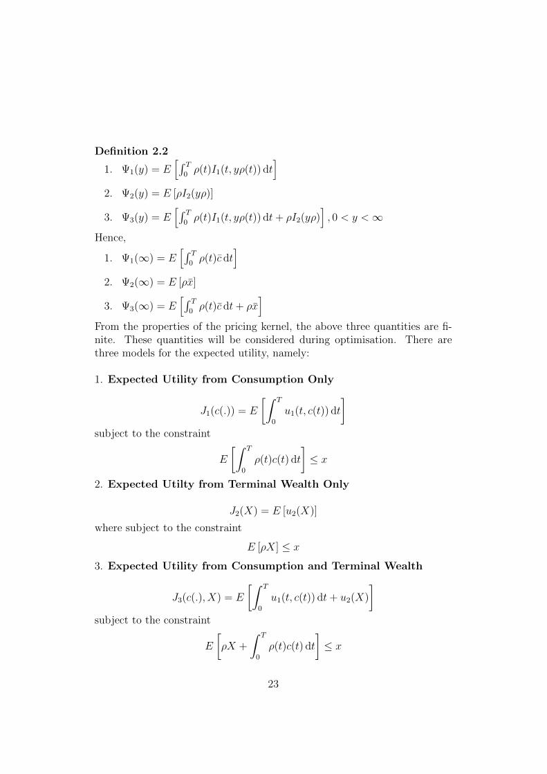
Definition 2.2

1. Ψ1(y) = E[∫ T

0ρ(t)I1(t, yρ(t)) dt

]2. Ψ2(y) = E [ρI2(yρ)]

3. Ψ3(y) = E[∫ T

0ρ(t)I1(t, yρ(t)) dt+ ρI2(yρ)

], 0 < y <∞

Hence,

1. Ψ1(∞) = E[∫ T

0ρ(t)c dt

]2. Ψ2(∞) = E [ρx]

3. Ψ3(∞) = E[∫ T

0ρ(t)c dt+ ρx

]From the properties of the pricing kernel, the above three quantities are fi-nite. These quantities will be considered during optimisation. There arethree models for the expected utility, namely:

1. Expected Utility from Consumption Only

J1(c(.)) = E

[∫ T

0

u1(t, c(t)) dt

]subject to the constraint

E

[∫ T

0

ρ(t)c(t) dt

]≤ x

2. Expected Utilty from Terminal Wealth Only

J2(X) = E [u2(X)]

where subject to the constraint

E [ρX] ≤ x

3. Expected Utility from Consumption and Terminal Wealth

J3(c(.), X) = E

[∫ T

0

u1(t, c(t)) dt+ u2(X)

]subject to the constraint

E

[ρX +

∫ T

0

ρ(t)c(t) dt

]≤ x

23

2.2 Behavioural Elements

2.2.1 S-Shaped Value Function and Probability Dis-tortions

Having formulated the problems for the neoclassical cases, we now move onto the behavioural aspect. As discussed, in order to incorporate the psycho-logical factors into the neoclassical finance model, to account for differentattitudes towards risk, non linear preferences etc, we need to introduce ourS-shaped value function and non-linear probability distortions.

Instead of a globally convex utility function as used in the conventional EUMmodel, we utilise a function, encapsulating the risk preferences dictated byCPT, which has a reference point B at terminal time T separating regionswhere terminal wealth is interpreted as gains (excess over B) and losses(shortfall from B). The reference point B is an FT -measurable random vari-able with E(ρB) < +∞. The functions u+ : <+ → <+ and u− : <+ → <+

are utility functions which measure the gains and losses respectively. Theyare both strictly increasing, concave and u+(0) = u−(0) = 0. u+(.) is strictlyconcave and twice differentiable, with u′+(0+) = +∞ and u′+(+∞) = 0.

Hence the agent value function

u(x) = u+(x+)1x≥0(x)− u−(x−)1x<0(x) (2.23)

where a+ denotes the positive part and a− denotes the negative part of areal number a. Combined in this form, we see that this captures the riskseeking and risk averse attitude towards gains and losses respectively, viathe S-shaped function, when x is negative, the function in this region isconvex, and when x is positive, the function in this region is concave.

Our non-linear probability distortions for gains and losses will be representedby the two functions w+ : [0, 1] → [0, 1] and w− : [0, 1] → [0, 1] respectively.Both of them are differentiable and strictly increasing, with w+(0) = w−(0) =0 and w+(1) = w−(1) = 1.

2.2.2 Formulating the Behavioural Criterion

Now, for the value of a contingent claim, CPT treated only the discrete case,so now we present the continuous case as used in [7]; given a contingent claimX, an FT -measurable random variable, we denote V (X) to be its value, and

24

it is defined as:

V (X −B) = E[u(X −B)] = V+((X −B)+)− V−((X −B)−) (2.24)

where, for any random variable Y ≥ 0, V+(.) and V−(.) are defined as:

V+(Y ) =

∫ ∞0

w+(Pu+(Y ) > y) dy, V−(Y ) =

∫ ∞0

w−(Pu−(Y ) > y) dy

(2.25)We have mentioned in chapter 1 that B can be assumed to be 0, so ourproblem is:

V (X) = E[u(X)] = V+(X+)− V−(X−) (2.26)

25

Chapter 3

Utility from Terminal Wealth

In this chapter, we will aim to solve the problem of expected utility maximi-sation from terminal wealth only subject to constraints which we will describelater. We will first review the neoclassical case with no probability distor-tions and a global concave utility function, and solve it before looking at thebehavioural case where probability distortions are present and we utility theS-shaped value function.

3.1 Neoclassical Problem

Problem Statement

Maximise :V2(x) = sup(c,π)∈A2(x)

J2(X) = sup(c,π)∈A2(x)

E [u2(X)] (3.1)

s.t. :

E [ρX] = xA2(x) = (c, π) ∈ A(x) : Emin[0, u2(X)] > −∞

where X = Xx,π,c is the terminal wealth with a given initial endowmentx ≥ 0 with associated portfolio process π(.) and consumption process c(.),u2(.) is the utility function, A2(x) = (c, π) ∈ A(x) : Emin[0, u2(X)] > −∞and A(x) is the set of admissible consumption-portfolio pairs.

Solution

We will proceed to solve the EUM for terminal wealth for the neoclassicalcase first, recall definition 2.1,

Ψ2(y) = E [ρI2(yρ)] ,Ψ2(∞) = E [ρx] (3.2)

26

where I2(.) is the inverse of the marginal utility u′2 and the quantity Ψ2(y) <∞,∀y ∈ (0,∞). Hence, Ψ2(y) is non-increasing and continuous on (0,∞),and strictly decreasing on (0, r2) where r2 is defined as,

r2 = supy > 0 : Ψ2(y) > Ψ2(∞) > 0 (3.3)

If we restrict the argument of the function Ψ2 to (0, r2) then it will have astrictly decreasing inverse function Φ2, hence, by definition,

Ψ2(Φ2(x)) = x,∀x ∈ (Ψ2(∞),∞) (3.4)

In view of theorem 2.2, the problem (3.1) can be essentially restated as:

Maximise :E [u2(ξ)] (3.5)

s.t. :

E [ρξ] = xξ is an a.s. lower bounded FT -measurable random variable

This problem may be tackled using the method of Lagrangian multipliersyielding,

= E [u2(ξ)]− y (E [ρξ]− x)

= xy + E[u2(ξ)− yρξ]≤ xy + E [u2(yρ)]

(3.6)

where the inequality arose from the convex dual, whose definition is givenas (2.19) u(y) ≥ u(x) − xy. By definition of the respective convex duals,equality holds, if and only if,

ξ∗ = (u′2)−1(yρ) = I2(yρ) (3.7)

We may find the value of the Lagrange multiplier y by substituting theseoptimal values into the contraint equation E[ρξ∗] = x, which, recalling (3.2)and (3.4), gives,

Ψ2(y) = E[ρI2(yρ)] = x

y = Φ2(x)

Therefore, the optimal quantities are,

ξ∗(x) = I2(Φ2(x)ρ)

Hence, when ξ∗(x) = Xx,c,π∗(x) = X∗(x)

V2(x) = E [u2(X∗(x))] (3.8)

27

3.2 Behavioural Problem

Having looked at the neoclassical case, we now introduce the S-shaped valuefunction and probability distortions. However, first we need to look at theissue of ill-posedness before we proceed.

3.2.1 Ill-Posedness

An EUM problem is said to be ill-posed if the optimal value for the problemis not finite. In EUT, the utility function is globally concave, enabling theproblem to be well-posed, i.e. have a finite optimal value, for most cases.However, since we wish to use a function which contains convex and concaveregions, coupled with non-linear probability distortions, ill-posedness is nowan issue and conditions must be enforced in order achieve well-posedness.

The following theorems are established in [7], and serve as a good basis forwell-posedness conditions.

Theorem 3.1(Jin & Zhou 2008 [7] Th. 3.1 and 3.2)The above maximisation problem is ill-posed under either of the followingtwo conditions:

1. There exists a non-negative FT -measurable random variable X suchthat E(ρX) < +∞ and V+(X) = +∞

2. u+(+∞) = +∞, ρ = +∞ and w−(x) = x

The first point is intuitive because it essentially states that the model isill-posed if the non-negative contingent claim has a finite price yet it hasan infinite prospective value, which means that the agent may purchase theclaim which has a finite price, but yet be able to attain an infinite value atthe end.

The second point shows that the utility on gains can be infinitely large, then aprobability distortion on losses is necessary in order to ensure well-posedness.Now we move onto the case where we utilise probability distortions and S-shaped functions as defined at the end of the previous chapter assumingthe conditions outlined in theorem 3.1. The problem with purely terminalwealth has been addressed in literature [7] so we will merely review the mainsteps. Take note that previously, we have used the term x to represent theinitial endowment, but now, to avoid unnecessary cumbersome notation, theinitial endowment for this single behavioural problem will be denoted x0. In

28

essence, we wish to solve the following maximisation problem:

Problem Statement

Maximise :V (X) =

∫ ∞0

w+(Pu+(X+) > y) dy +

∫ ∞0

w−(Pu−(X−) > y) dy

(3.11)

s.t. :

E[ρX] = x0

X is an a.s. lower bounded, FT -random variable

where u+ and u− are functions which map <+ → <+ forming our S-shapedvalue function given in (2.23) and w+ and w− are the probability distortionsmapping [0, 1] → [0, 1]. In this optimisational problem, X is the decisionvariable. Once optimal X∗ is obtained, the optimal portfolio is then theone replicating X∗. The quantity we wish to maximise contains probabilitydistortions reflecting on the subjective attitudes and the constraint doesn’t,because constraints are objective issues.

Solution

The key idea to tackling problem (3.11) is by breaking it down into threesub-problems. For any feasible solution X in (3.11), X+ corresponds to thegain in the event A = X ≥ 0 with replication cost x+ = E[ρX+] and X−

corresponds to the loss in the event Ac = X < 0 with E[ρX−] = x+ − x0.We wish to maximise V (X) = V+(X+) − V−(X−) so the idea is to splitthe problem into components; we firstly consider V+(X) which is a quantityrelating to gains so we wish to maximise V+(X) subject to constraints, thenwe consider V−(X), a quantity relating to the measurement of losses so wewish to minimise V−(X). If v+(A, x+) and v−(A, x+) are the maximal andminimal values for V+(X) and V−(X) respectively, then the next sub-problemis to maximise v+(A, x+)− v − (A, x+). Now we look at the sub-problems:

Sub-Problem 1

Maximise :V+(X) =

∫ ∞0

w+(Pu+(X) > y) dy (3.12)

s.t. :

E(ρX) = x+

X ≥ 0 a.s., x = 0 a.s. on Ac

29

This first sub-problem focuses on the V+(X) quantity in V (X) = V+(X+)−V−(X−) and the parameters are A ∈ FT and x+ ≥ x+

0 ≥ 0. It addresses theevent where our terminal wealth X is a gain so we aim to maximise this andour decision variable is X. The optimal value of this problem is denotedv+(A, x+) and is defined as follows:

1. P (A) > 0 =⇒ the feasible region for (3.12) is non-empty andv+(A, x+) is the supremum of V+(X)

2. P (A) = 0 and x+ = 0 =⇒ X = 0 and v+(A, x+) = 0

3. P (A) = 0 and x+ > 0 =⇒ there is no feasible solution for (3.12)v+(A, x) = −∞

Sub-Problem 2

Minimise :V−(X) =

∫ ∞0

w−(Pu−(X) > y) dy (3.13)

s.t. :

E(ρX) = x+ − x0, x ≥ 0 a.s., X = 0 a.s. on AX is upper bounded a.s.

The second sub-problem focuses on the V−(X) quantity in V (X) = V+(X+)−V−(X−) and the parameters are A ∈ FT amd x+ ≥ x+

0 ≥ 0 with X upperbounded. It addresses the event where our terminal wealth X is a loss so weaim to minimise this and our decision variable here is again X. The optimalvalue of this problem is denoted v−(A, x+) and is defined as follows:

1. P (A) < 1 =⇒ the feasible region of (3.13) is non-empty and v−(A, x+)is the infimum of V−(X)

2. P (A) = 1 and x+ = x0 =⇒ X = 0 and v−(A, x+) = 0

3. P (A) = 1 and x+ 6= x0 =⇒ v−(A, x) = +∞

Sub-Problem 3

Maximise :v+(A, x+)− v−(A, x+) (3.14)

s.t. :

A ∈ FT x+ ≥ x+

0

x+ = 0 when P (A) = 0, x+ = x0 when P (A) = 1

In this third sub-problem, we wish to find the optimal split between thequantities which relate to gains and losses. The decision variables in thismaximisation problem here are x+, a real number and A, a random event.The random event A causes difficulty in approaching this problem so in [7],

30

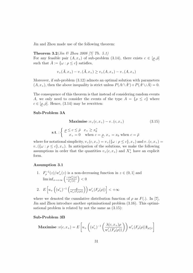
Jin and Zhou made use of the following theorem:

Theorem 3.2(Jin & Zhou 2008 [7] Th. 5.1)For any feasible pair (A, x+) of sub-problem (3.14), there exists c ∈ [ρ, ρ]

such that A := ω : ρ ≤ c satisfies,

v+(A, x+)− v−(A, x+) ≥ v+(A, x+)− v−(A, x+)

Moreover, if sub-problem (3.12) admots an optimal solution with parameters(A, x+), then the above inequality is strict unless P (A∩ Ac)+P (Ac∪ A) = 0.

The consequence of this theorem is that instead of considering random eventsA, we only need to consider the events of the type A = ρ ≤ c wherec ∈ [ρ, ρ]. Hence, (3.14) may be rewritten:

Sub-Problem 3A

Maximise :v+(c, x+)− v−(c, x+) (3.15)

s.t. :

ρ ≤ c ≤ ρ x+ ≥ x+

0

x+ = 0 when c = ρ, x+ = x0 when c = ρ

where for notational simplicity, v+(c, x+) = v+(ω : ρ ≤ c, x+) and v−(c, x+) =v−(ω : ρ ≤ c, x+). In anticipation of the solutions, we make the followingassumptions in order that the quantities v+(c, x+) and X∗+ have an explicitform.

Assumption 3.1

1. F−1ρ (z)/w′+(z) is a non-decreasing function in z ∈ (0, 1] and

lim infx→+∞

(−xu′′+(x)

u′+(x)

)< 0

2. E[u+

((u′+)−1

(ρ

w′+(Fρ(ρ))

))w′+(Fρ(ρ))

]< +∞

where we denoted the cumulative distribution function of ρ as F (.). In [7],Jin and Zhou introduce another optimisational problem (3.16). This optimi-sational problem is related by not the same as (3.15):

Sub-Problem 3B

Maximise :v(c, x+) = E

[u+

((u′+)−1

(λ(c, x+)ρ

w′+(Fρ(ρ))

))w′+(Fρ(ρ))1ρ≤c

]

31

−u−(x+ − x0

E[ρ1ρ>c]

)w−(1− Fρ(c)) (3.16)

s.t. :

ρ ≤ c ≤ ρ x+ ≥ x+

0

x+ = 0 when c = ρ, x+ = x0 when c = ρ

where λ(c, x+) satisfies E[(u′+)−1( λ(c,x+)ρ

w′+(Fρ(ρ)))ρ1ρ≤c

]= x+ and using the con-

vention that u−

(x+−x0E[ρ1ρ>c]

)w−(1− Fρ(c)) = 0 when c = ρ and x+ = x0

Jin and Zhou [7] proved that (3.15) and (3.16) have the same supremumvalues hence if we solve (3.16) we also obtain the solution for (3.15). Theproblem of finding the optimal quantities for expected utility maximisationfor terminal wealth in the behavioural context has been calculated in litera-ture [7] and the results are presented in the proceeding theorem.

Theorem 3.1(Jin & Zhou 2008 [7] Th. 4.1)Under assumptions (3.1) and assuming that u−(.) is strictly concave at 0:

1. IfX∗ is optimal for (3.11), then c∗ = F−1ρ (PX∗ ≥ 0), x∗+ = E[ρ(X∗)+],

where Fρ(.) is the cumulative distribution function for ρ are optimalfor (3.16).

2. If (c∗, x∗+) is optimal for (3.16) problem and X∗+ is optimal for (3.12)with parameters (ρ ≤ c∗, x∗+), then

X∗ =

[(u′+)−1

(λ(c∗, x∗+)ρ

w′+(Fρ(ρ))

)]1ρ≤c∗ −

[x∗+ − x0

E[ρ1ρ>c∗ ]

]1ρ>c∗ (3.17)

is optimal for (3.11), where λ(c, x+) satisfies E[(u′+)−1( λ(c,x+)ρ

w′+(Fρ(ρ)))ρ1ρ≤c

]= x+

and Fρ(.) is the cumulative density function for the terminal state pricingkernel.

This explicit form of terminal wealth (3.17) tells us that whether the agentperceives the terminal wealth as a gain or a loss is determined by c∗ : ifthe terminal state pricing density is less than or equal to c∗ then the agentperceives a gain and if the terminal state pricing density is bigger than the c∗,then a perceived loss is attained. So the probability of attaining a perceivedgain is given by P (ρ ≤ c∗) = Fρ(c

∗)[3].

In order to replicate this optimal terminal value, at time 0, the agent buys a

contingent claim with payoff[(u′+)−1

(λ(c∗,x∗+)ρ

w′+(Fρ(ρ))

)]1ρ≤c∗ at cost x∗+. However,

32

since x∗+ ≥ x0 the agent will also need to sell a claim at cost x∗+ − x0 with

payoff[

x∗+−x0E[ρ1ρ>c∗ ]

]1ρ>c∗ to fund her purchase.

The case considered here was when the reference point B = 0. The generalform [3]when B 6= 0 is:

X∗ =

[(u′+)−1

(λ(c∗, x∗+)ρ

w′+(Fρ(ρ))

)+B

]1ρ≤c∗ −

[x∗+ − (x0 − E[ρB])

E[ρ1ρ>c∗ ]−B

]1ρ>c∗

where c∗ := F−1ρ (PX∗ ≥ B), x∗+ = E[ρ(X∗ − B)+] and λ(c, x+) satisfies

E[(u′+)−1( λ(c,x+)ρ

w′+(Fρ(ρ)))ρ1ρ≤c

]= x+ and Fρ(.).

33

Chapter 4

Utility from Consumption &Terminal Wealth

In this chapter, we will aim to solve the problem of expected utility maximi-sation from terminal wealth and consumption subject to constraints whichwe will describe later. We will first review the neoclassical case with no prob-ability distortions and a global concave utility function, and solve it beforelooking at the behavioural case where probability distortions are present andthe utility is an S-shaped value function.

4.1 Neoclassical Problem

Problem Statement

Maximise :V3(x) = sup(c,π)∈A3(x)

E

[∫ T

0

u1(t, c(t)) dt+ u2(X)

](4.1)

s.t. :

E[ρX +

∫ T0ρ(t)c(t) dt

]= x

A3 = A1(x) ∩ A2(x)

where X = Xx,π,c is the terminal wealth with a given initial endowment x ≥ 0with associated portfolio process π(.) and consumption process c(.), u1(.) and

u2 are utility functions, A1(x) = (c, π) ∈ A(x) : Emin[0,∫ T

0u1(t, c(t))] dt >

−∞ A2(x) = (c, π) ∈ A(x) : Emin[0, u2(X)] > −∞, A3 = A1(x) ∩ A2(x)and A(x) is the set of admissible consumption-portfolio pairs

Solution

Again, we will start from the conventional EUM for maximising expected

34

utility with consumption and terminal wealth. Recall definition 2.1,

Ψ3(y) = E

[∫ T

0

ρ(t)I1(t, yρ(t)) dt+ ρI2(yρ)

],Ψ3(∞) = E

[∫ T

0

ρ(t)c dt+ x

](4.2)

where I1(.) and I2(.) are the inverses of the marginal utilities u′1 and u′2respectively and the quantity Ψ3(y) <∞,∀y ∈ (0,∞). Hence, Ψ3(y) is non-increasing and continuous on (0,∞), and strictly decreasing on (0, r3) wherer3 is defined as,

r3 = supy > 0 : Ψ3(y) > Ψ3(∞) > 0 (4.3)

If we restrict the argument of the function Ψ3 to (0, r3) then it will have astrictly decreasing inverse function Φ3, hence, by definition,

Ψ3(Φ3(x)) = x,∀x ∈ (Ψ3(∞),∞) (4.4)

As usual, in view of theorem 2.2, the problem (4.1) can be essentially restated:

Maximise :E

[∫ T

0

u1(t, c(t)) dt+ u2(ξ)

](4.5)

s.t. :

E[∫ T

0ρ(t)c(t) dt+ ρξ

]= x ≥ 0

ξ is an a.s. bounded FT measurable random variable

where c(.) is the consumption process, and u1(.) and u2(.) are utility func-tions. This problem may be tackled using the method of Lagrangian multi-pliers yielding,

= E

[∫ T

0

u1(t, c(t)) dt+ u2(ξ)

]− y

(E

[∫ T

0

ρ(t)c(t) dt+ ρξ

]− x)

= xy + E

∫ T

0

[u1(t, c(t))− yρ(t)c(t)] dt+ E[u2(ξ)− yρξ]

≤ xy + E

[∫ T

0

u1(t, yρ(t)) dt+ u2(yρ)

](4.6)

where the inequality arises from the convex dual which, by definition of therespective convex duals, equality holds, if and only if,

c∗(t) = (u′1)−1(t, yρ(t)) = I1(t, yρ(t)), ξ∗ = (u′2)−1(yρ) = I2(yρ) (4.7)

35

for 0 ≤ t ≤ T . We may find the value of the lagrange multiplier y by substi-

tuting these optimal values into the contraint equation E[∫ T

0ρ(t)c∗(t) dt+ ρξ∗

]=

x, which, using (4.2) and (4.4), gives,

Ψ3(y) = E

[∫ T

0

ρ(t)I1(t, yρ(t)) dt+ ρI2(yρ)

]= x

y = Φ3(x)

(4.8)

Therefore, the optimal quantities are,

c∗t (x) = I1(t,Φ3(x)ρ(t)), ξ∗(x) = I2(Φ3(x)ρ) (4.9)

Hence, when ξ∗(x) = Xx,c,π∗(x) = X∗(x)

V3(x) = E

[∫ T

0

u1(t, c∗t (x)) dt+ u2(X∗(x))

](4.10)

4.2 Behavioural Problem

Our conventional problem was V3(x) = sup(c,π)∈A3(x) E[∫ T

0u1(t, c(t)) dt+ u2(X)

],

however, due to the non-linearity of distorted expectation, when looking atEUM with terminal wealth and consumption from a behavioural point ofview, we have three cases which we may consider:

Problem 1

E

(∫ T

0

u1(c(t)) dt+ u2(X)

)(4.11)

Problem 2

E

(∫ T

0

u1(c(t)) dt

)+ E [u2(X)] (4.12)

Problem 3 ∫ T

0

E (u1(c(t))) dt+ E[u2(X)] (4.13)

Each of these problems fall under the terminal wealth and consumption cat-egory but the one which is taken onboard by the majority remains open fordiscussion. (4.11) resembles the case where an agent considers the terminalwealth and their consumption process as a whole, (4.12) resembles the casewhere an agent wishes to maximise their terminal wealth and consumption

36

process separately but considers their overall consumption through the hori-zon [0, T ] and (4.13) is similar to problem 2, only the agent considers theirconsumption “incrementally” as opposed to overall.

These three problems are all subject to the contraint E(∫ T

0c(t)ρ(t) dt+ρX) =

x0. Out of these three problems, (4.12) and (4.13) seem more realistic aspeople usually wish to plan their terminal wealth and consumption processseparately although this requires empirical evidence to support this claim.Agents may also anticipate unexpected changes throughout their consump-tion process and so, may prefer to maximise their subjective expectation forconsumption for all time, rather than throughout the entire time horizon[0, T ], hence for these reasons, we will explore (4.13). Like in the previouschapter in the behavioural problem section, we wish to denote our initialendowment by x0. Hence our maximisation problem is:

Problem Statement

Maximise :

[∫ T

0

E[u1(c(t))] dt+ Eu2(X)

](4.14)

s.t. :

E(∫ T

0c(t)ρ(t) dt+ ρX

)= x0

c(t) ≥ 0, X is an a.s. lower bounded, FT random variable

where u1(.) and u2(.) are S-shaped value functions, E(.) is the distortedexpectation operator capturing subjective decision making and E(.) is thenormal expectation operator.

Solution

We shall tackle this problem by splitting the quantities up, so our problem,∫ T0Eu(c(t)) dt+ Eu(X) subject to

∫ T0E(c(t)ρ(t)) dt+ E(ρX) = x0, may be

divided when we allocate our initial endowment x0 into two funds; one tofund the quantity to achieve our desired consumption which we denote x1

and the other one to fund the quantity to achieve our desired terminal wealthwhich we denote x2, hence x1 + x2 = x0. Consequently, we have two sub-problems; problem (4.15) deals with the consumption aspect, whilst problem(4.16) deals with the terminal wealth aspect.

37

Sub-Problem 1:

Maximise :V1(c(t)) = max

[∫ T

0

Eu1(c(t)) dt

](4.15)

s.t. :

∫ T

0

E(c(t)ρ(t)) dt = x1 ≥ 0, c(t) ≥ 0

Sub-Problem 2:

Maximise :V2(X) =[Eu2(X)

](4.16)

s.t. :

E(ρX) = x2 ≥ 0X is an a.s. lower bounded, FT random variable

(4.16) has already been addressed in the previous chapter so the optimalvalue for (4.16) is:

X∗ =

[(u′2+)−1

(λ(c∗, x∗+)ρ

w′+(Fρ(ρ))

)]1ρ≤c∗ −

[x∗+ − x2

E[ρ1ρ>c∗ ]

]1ρ>c∗

where x∗+ is the price of terminal gains and λ(c, x+) satisfiesE[(u′2+)−1( λ(c,x+)ρ

w′+(Fρ(ρ)))ρ1ρ≤c

]=

x+. Hence we only need to consider (4.15). This problem can be solved bysplitting it further into two sub-problems:

Sub-Problem 1A:

Maximise : maxc(t)

E[u1(c(t))] (4.17)

s.t. :

E(c(t)ρ(t)) = b(t)

c(t) ≥ 0

where ρ(t) is a given strictly positive random variable, with no atom whosecumulative distribution function is given as Fρ(t)(.). We denote the optimalvalue for this problem as v[b(t)]. c(t) is the consumption process and thedecision variable here with parameter b(t).

38

Sub-Problem 1B:

Maximise :

∫ T

0

v[b(t)] dt (4.18)

s.t. :

∫ T0b(t) dt = x1

b(t) ≥ 0

Here, b(t) is the decision variable. We proceed by solving (4.17) then (4.18).In order to solve (4.17), we need to employ a technique known as quantileformulation in order to tame the distorted expectation into a more manipu-latable form [46]. Now c(t) ≥ 0 a.s., so we treat it as a non-negative randomvariable. Furthermore, recall (2.23) the definition of our S-shaped value func-tion u(x) = u+(x+)1x≥0(x)−u−(x−)1x<0(x), for x ∈ <. Now for u(c(t)),sincec(t) is positive, we need only concern ourselves with the positive part and so,by definition,

Eu1(c(t)) =

∫ +∞

0

wP (u1(c(t)) > y) dy

where w : [0, 1] → [0, 1] is a strictly increasing, differentiable function withw(0) = 0, w(1) = 1 and u(.) is a strictly concave, strictly increasing, twicedifferentiable function with u(0) = 0, u′(0) = +∞, u′(+∞) = 0. For (4.17)since c(t) is considered for one time only, we condense the notation from c(t)to ct and ρ(t) to ρt. Now, our maximisation problem may be rewritten as:

Maximise :α1(ct) =

∫ +∞

0

wP (u1(ct) > y) dy (4.19)

s.t. :E[ρtct] = bt ≥ 0, c(t) ≥ 0

The probability distortion w(.) in α1(ct) means that it is not globally concaveor convex in ct. Quantile formulation, the technique which we will employ,changes the decision variable from ct to it’s quantile function which we denoteG(.), the effect of this transformation is that concavity is recovered.

Now if we have two random variables X and Y , and X ∼ Y then α(X) =α(Y ) by the law-invariance property of α(.) [3]. Let Z := 1−Fρt(ρt), implyingthat Z ∼ U(0, 1) and hence, because ρ(t) is assumed to be atomless, wemay rearrange the equation, we have, ρt = F−1

ρt (1 − Z) a.s.[46]. Let Gbe the quantile function of a non-negative random variable such that G isnon-decreasing with G(0−) = 0 and G(+∞) = 1. It is proved in [7] thatif (4.19) admits an optimal solution c(t)∗ whose quantile function is G(.),

39

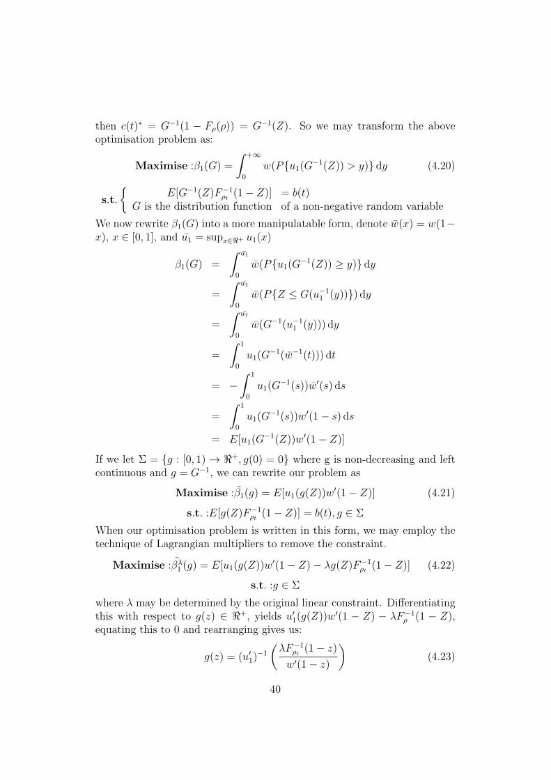
then c(t)∗ = G−1(1 − Fρ(ρ)) = G−1(Z). So we may transform the aboveoptimisation problem as:

Maximise :β1(G) =

∫ +∞

0

w(Pu1(G−1(Z)) > y) dy (4.20)

s.t.

E[G−1(Z)F−1

ρt (1− Z)] = b(t)G is the distribution function of a non-negative random variable

We now rewrite β1(G) into a more manipulatable form, denote w(x) = w(1−x), x ∈ [0, 1], and u1 = supx∈<+ u1(x)

β1(G) =

∫ u1

0

w(Pu1(G−1(Z)) ≥ y) dy

=

∫ u1

0

w(PZ ≤ G(u−11 (y))) dy

=

∫ u1

0

w(G−1(u−11 (y))) dy

=

∫ 1

0

u1(G−1(w−1(t))) dt

= −∫ 1

0

u1(G−1(s))w′(s) ds

=

∫ 1

0

u1(G−1(s))w′(1− s) ds

= E[u1(G−1(Z))w′(1− Z)]

If we let Σ = g : [0, 1) → <+, g(0) = 0 where g is non-decreasing and leftcontinuous and g = G−1, we can rewrite our problem as

Maximise :β1(g) = E[u1(g(Z))w′(1− Z)] (4.21)

s.t. :E[g(Z)F−1ρt (1− Z)] = b(t), g ∈ Σ

When our optimisation problem is written in this form, we may employ thetechnique of Lagrangian multipliers to remove the constraint.

Maximise :βλ1 (g) = E[u1(g(Z))w′(1− Z)− λg(Z)F−1ρt (1− Z)] (4.22)

s.t. :g ∈ Σ

where λ may be determined by the original linear constraint. Differentiatingthis with respect to g(z) ∈ <+, yields u′1(g(Z))w′(1 − Z) − λF−1

ρ (1 − Z),equating this to 0 and rearranging gives us:

g(z) = (u′1)−1

(λF−1

ρt (1− z)

w′(1− z)

)(4.23)

40

It may be verified that this quantity is indeed a maximum because if wedifferentiate again, we get u′′1(g(Z))w′(1− Z), since u1(.) is concave, u′′1(.) <0 and also w′(.) > 0, hence the second derivative is a negative quantityindicating the function g(z) yields a maximum. As mentioned above g = G−1

must be non-decreasing, so if F−1ρt (z)/w′(z) is non-decreasing in z ∈ (0, 1],

then g(z) is non-decreasing in z ∈ [0, 1) which satisfies the conditions requiredto be a solution for the above maximisation problem otherwise, it doesn’t.In the previous chapter, it was an assumption that F−1

ρt (z)/w′(z) is non-decreasing in z ∈ (0, 1] hence, with this assumption, optimal g is guaranteed.Rewriting and summarising the calculations, we have:

Maximise : maxc(t)

Eu1(c(t))

s.t. :

E(c(t)ρ(t)) = b(t)

c(t) ≥ 0

and since Z = 1− Fρ(ρ),

c∗t (λ) = (u′1)−1

(λρt

w′(Fρt(ρt))

), λ > 0 (4.24)

where λ satisfies E(ρtc∗t (λ)) = bt, hence λ = f [b(.)]. Having attained the

optimal solution for (4.17) we now we wish to solve problem (4.18):

Maximise :

∫ T

0

v[b(t)] dt

s.t. :

∫ T0b(t) dt = x1

b(t) ≥ 0

Again, we apply the Lagrangian method to get rid of the contraint, by intro-ducing the Lagrangian multiplier φ

Maximise :

∫ T

0

v[b(t)] dt− φ∫ T

0

b(t) dt− x1 (4.25)

Equivalently,

Maximise :

∫ T

0

v[b(t)]− φb(t) dt (4.26)

Differentiating the integrand with respect to b(t) and equating it to 0 yieldsv′[b∗(t)]− φ = 0 and therefore

41

b∗(t) = (v′)−1(φ) (4.27)

where φ satisfies∫ T

0(v′)−1(φ) dt = x1, hence φ = ψ(x1). Inserting this into

(4.27) gives:b∗(t) = (v′)−1(φ(x1)) (4.28)

Now for continuous random variable X ≥ 0,

v′(X) = E ′u1(X) =

∫ ∞0

w′(1− FX(y)) dy

= −∫ ∞

0

w′(1− FX(y))fX(y) dy

v′′(X) = E ′′u1(X)

=

∫ ∞0

w′′(1− FX(y))f 2X(y) dy −

∫ ∞0

w′(1− FX(y))dfX(y)

dxdy

Since w′(.) > 0, v′′(b(t)) < 0 implicating that the quantity b∗(t) is optimalfor the problem.

Combining the optimal solutions for the two subproblems (4.24) and (4.28),we find that the optimal value for problem 1 is:

c∗t (x1) = (u′1)−1

(f(v′)−1(ψ(x1))ρt

w′(Fρt(ρt))

)(4.29)

We conclude this consumption part with the following theorem which reas-sures us that our splitting process indeed solves our optimisational problem(4.15). We will then resume with our original problem of this subsection inthis chapter, optimising the expected utility with consumption and terminalwealth in the behavioural context.

Theorem 4.1

1. If c∗ is optimal for (4.15) then b∗(t) := E(c∗(t)ρ(t)) optimal for (4.18)and c∗(t) is optimal for (4.17) with b(.) = b∗(.)

2. If b∗(.) is optimal for (4.18) and c∗(.) is optimal for (4.17) with param-eters b(.) = b∗(.) then c∗ is optimal for (4.15)

42

Proof

1. (i) We wish to show that∫ T

0v[b(t)] dt ≤

∫ T0v[b∗(t)] dt, for all feasible

b(t) and b∗(t) := E(c∗(t)ρ(t)). For any b(.) there exists a c(.) such thatEu1(c(t)) = v(b(t)) ∀t ∈ [0, T ] and b(t) = E[c(t)ρ(t)]. Hence,∫ T

0

v[b(t)] dt =

∫ T

0

Eu1(c(t)) dt

≤ max

∫ T

0

Eu1(c(t)) dt

=

∫ T

0

Eu1(c∗(t)) dt

=

∫ T

0

v[b∗(t)] dt

(ii) Now we need to show that if c∗(t) is optimal for (4.15), then c∗(t) isoptimal for (4.17) with b(.) = b∗(.). c∗(t) is optimal for (4.15), hence,∫ T

0

E(u1(c(t))) dt ≤∫ T

0

E(u1(c∗(t))) dt

for all c(t) feasible for (4.15). Also, c∗(t) with b(.) = b∗(.) is feasible for (4.17)

E(u1(c(t))) ≤ E(u1(c∗(t)))

Eu1(ct) ≤ v[c∗(t)]

2. We need to show that if b∗(.) is optimal for (4.18) and c∗(t) is optimalfor (4.17) with b(.) = b∗(.) then c∗ is optimal for (4.15). For all c(.), defineb(.) = E[c(.)ρ(.)], then,∫ T

0

Eu1(c(t)) dt ≤∫ T

0

v[b(t)] dt

≤∫ T

0

v[b∗(t)] dt

=

∫ T

0

Eu1(c∗(t)) dx

as required.

43

Summarising, from (4.29) c∗t (x1) = (u′1)−1(f(v′)−1(ψ(x1))ρt

w′(Fρt (ρt))

)is the optimal

consumption, and X∗(x2) =[(u′2+)−1

(λ(c∗,x∗+)ρ

w′+(Fρ(ρ))

)]1ρ≤c∗ −

[x∗+−x2

E[ρ1ρ>c∗ ]

]1ρ>c∗ is

the optimal terminal wealth where where λ(c, x+) satisfies E[(u′2+)−1( λ(c,x+)ρ

w′+(Fρ(ρ)))ρ1ρ≤c

]=

x+ and x0 = x1 + x2. Our original problem was to solve:

Maximise :

[∫ T

0

E[u1(c(t))] dt+ Eu2(X)

]

s.t. :

E(∫ T

0c(t)ρ(t) dt+ ρX

)= x0 = x1 + x2

c(t) ≥ 0, X is an a.s. lower bounded, FT random variable

The ratio of x1 to x2 may be determined as follows, for a given x0, the optimalquantities c∗t (x1) and X∗(x0 − x1) are inserted into the above maximisationproblem, so that for a given x1,

γ(x1) = max

∫ T

0

E (u1(c∗t (x1))) dt+ E[u2(X∗(x0 − x1)) (4.30)

By recalling notation from (4.15) and (4.16) we write∫ T

0E (u1(c∗t (x1))) dt =

V1(x1) and E[u2(X∗(x0−x1)) = V2(x0−x1) hence we can neatly express theintegrand as V1(x1) + V2(x0 − x1). Finally, to solve the terminal value andconsumption maximisation problem, we work out:

γ(x1) = max0≤x1≤x0

V1(x1) + V2(x0 − x1) (4.31)

enabling us to work out the optimal splitting.

4.2.1 Algorithm

The main steps to solving (4.14) are outlined here,

1. Solve (4.15) with any x1 ≥ 0 to get optimal value V1(x1) and optimalconsumption c∗t (x1)

2. Solve (4.16) with any x2 ∈ < to get optimal value V2(x2) and optimalterminal wealth X∗(x2)

3. Solve (4.31) with V1(x1) and V2(x2) obtained in the previous steps

So now we have the following algorithm to solve problem (4.14).

44

Behavioural Expected Utility Maximisation with Consumption andTerminal Wealth Algorithm

1. Solve (4.17) for any b(t) ≥ 0 to get its optimal value function v[b(t)]and optimal solution c∗(b(t))

2. Plug v(.) to problem (4.18) and solve it to get the optimal solutionb∗(t).

3. c∗(t) = c∗(b∗(t)) gives an optimal solution to (4.15). Obtain V1(c∗t (x1))

4. Solve problem (3.12) with (ω : ρ ≤ c, x+), where ρ ≤ c ≤ ρ and x+ ≥x+

2 are given, to obtain v+(c, x+) and the optimal solution X∗+(c, x+)

5. Solve problem (3.16) to get (c∗, x∗+)

6. If (c∗, x∗+) = (ρ, x2) then X∗+(ρ, x2) solves (4.16) otherwise X∗(x2) =[(u′2+)−1

(λ(c∗,x∗+)ρ

w′+(Fρ(ρ))

)]1ρ≤c∗−

[x∗+−x2

E[ρ1ρ>c∗ ]

]1ρ>c∗ solves (4.16). Obtain V2(X∗(x2))

7. With x0 = x1 + x2, solve problem (4.31) to find the optimal split

45

Chapter 5

Conclusions

Expected Utility Maximisation was regarded as one of the crowning achieve-ments in optimal portfolio selection, however, the repeated violations in ob-servation evidently suggests that this is not an adequate model of decisionmaking under risk and uncertainty. Instead, EUT can be regarded more as acornerstone for our quest towards exploring the optimal portfolio problem, asmore empirical and theoretical research is conducted to close the gap betweenhow agents really make decision and what is dictated by the mathematics.

CPT is generally accepted as the descriptive model for risky decision making,and work is currently being done to “mathematicalised” this behavioural fi-nance concept. The psychological aspects are incorporated adequately; theonce globally concave utility function used in EUT, is replaced with an S-shaped value function, whose regions of convexity and concavity are dis-tinguished by a reference point, capturing the agents general risk attitudetowards gains and losses. Introducing the probability distortions also takesinto the notion that agents tend to overweigh small probabilities and under-weigh large probabilities.

The results of chapter 4 are:

c∗t (x1) = (u′1)−1

(f(v′)−1(ψ(x1))ρt

w′(Fρt(ρt))

)

X∗(x2) =

[(u′2+)−1

(λρ

w′2+(Fρ(ρ))

)]1ρ≤c∗ −

[x∗2+ − x2

E[ρ1ρ>c∗ ]

]1ρ>c∗

for x0 = x1 + x2 where x0 is the initial endowment. We also formulated analgorithm to solve this problem.

46

5.1 Possible Extensions

As we have outlined before in the previous chapter on maximising expectedutility with terminal wealth and consumption, if we introduce the behaviouralcriterion, this maximising problem may be interepreted in three differentways. The whole point of developing theories beyond EUT to behaviouralfinance was due to the fact that theory was not observed in practice. The psy-chological extensions were required to address these deviations, and hence,further research could be employed to see which of the three different in-tepretations, which all yield different values, most closely match real life.

Intuitively, out of the three problem intepretations, thought experimentsmight advocate the non existence of a general prevalent problem mainly dueto the fact that for any single agent, she might employ different subjectivemethods of considering her subjective expected utility to maximise so contextis very important. A simple example demonstrating this would be comparingthe scenario when the agent is drawing up a monthly spending budget, soshe wishes to plan her consumption over the time horizon and also wish tohave a certain amount to pay off, say the rent and another scenario wheresay the agent makes decisions Taoistically and “go with the flow”. (4.12)and (4.13) would probably be more suited to analysing the former and thelatter scenarios respectively.

Since context is important, one may wish to restrict the scenario and inves-tigate this problem in financial investment situations. As for mathematicalextensions, solving each of the three problems would stand as a challeng-ing problem itself as each would require different methods of deducing theoptimal quantities due to the nature of the non-linear expectations.

47

Bibliography

[1] Gove, P. et al. 1961. Finance. Webster’s Third New International Dictio-nary of the English Language Unabridged. Springfield, Massachusett : G.and C. Merriam Company

[2] Robert J. Shiller 2006. Financial Review, Vol. 41, No. 1, pp. 1-8, Febru-ary 2006. Tools for Financial Innovation: Neoclassical versus Behaviouralfinance. Cowles Foundation Paper No. 1180. Yale University - Cowles Foun-dation; National Bureau of Economic Research (NBER); Yale University -International Center for Finance

[3] Xun Yu Zhou 2010. Mathematicalising Behavioural Finance. Hyderabad,India 2010. Proceedings of the International Congress of Mathematicians2010 (ICM 2010) (pp 3185-3209)

[4] What is Behavioural Finance? (2000) Business, Education and Technol-ogy Journal, Vol. 2, No. 2, pp. 1-9, Fall 2000. Victor Ricciardi. GoucherCollege - Department of Business Management Helen K. Simon. FloridaInternational University (FIU) - Department of Finance; Personal BusinessManagement Services, LLC.

[5] Essentials of Investments 5th Edition (2004). Active Investment Man-agement Behavioural Finance and Technical Analysis. Zvi Bodie, BostonUniversity. Alex Kane, University of California, San Diego. Alan J. Marcus,Boston College. ISBN: 0072510773

[6] Behavioural Finance (2003). Jay R. Ritter. Cordell Professor of Finance.University of Florida. Published, with minor modifications, in the Pacific-Basin Finance Journal Vol. 11, No. 4, (September 2003) pp. 429-43

[7] Hanqing Jin and Xun Yu Zhou. Behavioural Portfolio Selection in Contin-uous Time, Mathematical Finance, 18 : 385-426, 2008. Erratum, To appear

48

in Mathematical Finance, 2010

[8] T. Copeland, F. Weston and K. Shastri (2005), Financial Theory andCorporate Policy, 4th Edition, Pearson Addision Wesley.

[9] Ellsberg, Daniel. (1954). ”Classic and current notions of ’Measurableutility’”. Economic Journal 64(255) : 528-556

[10] Salvador Barbera, Peter J. Hammond, Christian Seidl (1998). Handbookof Utility Theory, Volume 2. ISBN 0-7923-8174-2

[11] Paul J. H. Schoemaker (1982). Journal of Economics Literature. Coverage :1969-2008 (Vols. 7-46) Vol. XX, pp. 529-563. The Expected Utility Model :Its Variants, Purposes, Evidence and Limitations

[12] Daniel Bernoulli (1954). Exposition of a New Theory on the Measure-ment of Risk. Econometrica, Vol. 22, No. 1, pp. 23-36

[13] John Von Neumann and Oskar Morgenstern (1953). Theory of Gamesand Economic Behaviour. Princeton University Press

[14] Peter C. Fishburn (1989). Retrospective on the Utility Theory of vonNeumann and Morgenstern. Journal of Risk and Uncertainty, 1989, Vol. 2,Issue 2, pages 127-57

[15] EconPort Current Development 2006. Von Neumann-Morgenstern Ex-pected Utility Theory. Decisions Under Uncertainty. Georgia State Univer-sity. Experimental Economics Center. http: //www.econport.org

[16] Jonathan E. Ingersoll, Jr. Theory of Financial Decision Making. Row-man and Littlefield, 1987. p. 21

[17] Peter C. Fishburn (1975). Axioms for Lexicographic Preferences. TheReview of Economic Studies. Coverage : 1933-2007 (Vols. 1-74)

[18] Robin P. Cubitt, Chris Starmer, Robert Sugden (2001). Discovered pref-erences and the experimental evidence of violations of expected utility theory.Journal of Economic Methodology. Volume 8, Issue 3, 2001, Pages 385 - 414

[19] Maurice Allais (1953). Le comportement de lhomme rationnel devant lerisqu: critique des postulats et axioms de lecole Amricaine. Econometrica

49

21, pages 503-546.

[20] Daniel Kahneman and Amos Tversky (1979). Prospect Theory: AnAnalysis of Decision under Risk. Econometrica 47, Pages 263-291

[21] M.H.Michael H. Birnbaum (2004). Causes of Allais common consequenceparadoxes : An experimental dissection. Journal of Mathematical Psychol-ogy Volume 48, Issue 2, April 2004, Pages 87-106

[22] Ellsberg, Daniel (1961). ”Risk, Ambiguity, and the Savage Axioms”.Quarterly Journal of Economics 75 (4) : 643669

[23] Hersh Shefrin and Meir Statman (2000). Behavioural Portfolio Theory.Journal of Financial and Quantitative Analysis. Vol 35. No 2. School ofBusiness Administration, University of Washington, Seattle

[24] Mehra, Rajnish; Edward C. Prescott (1985). ”The Equity Premium: APuzzle” (PDF). Journal of Monetary Economics 15 (2) : 145161.

[25] Amos Tversky and Daniel Kahneman (1992). Advances in ProspectTheory: Cumulative Representation of Uncertainty. Journal of Risk andUncertainty, 5 : pages 297-323

[26] William T. Harbaugh, Kate Krause and Lise Vesterlund (2009). TheFourfold Pattern of Risk Attitudes in Choice and Pricing Tasks. The Eco-nomic Journal. Royal Economic Society

[27] Harry Markowitz (1952). The Utility of Wealth. The Journal of PoliticalEconomy, Vol. 60, No. 2. (Apr.,1952), pp.151-158.

[28] Amos Tversky and Peter Wakker (1995). Risk Attitudes and DecisionWeights. Econometrica Vol 63, No. 6, Nov., 1995 pages 1255-1280

[29] Amos Tversky and Daniel Kahneman (1984). Choices, values, andframes. 1983 APA Award Addresses

[30] Jack S. Levy (1996). Loss Aversion, Framing, and Bargaining: TheImplications of Prospect Theory for International Conflict. InternationalPolitical Science Review 1996 17: 179

[31] Amos Tversky and Daniel Kahneman (1991). Loss Aversion in Riskless

50

Choice : A Reference-Dependent Model. The Quarterly Journal of Eco-nomics (1991) 106(4) : 1039-1061

[32] Kenneth J Arrow (1951). Alternative Approaches to the Theory ofChoice in Risk Taking Situations. Econometrica, Hournal of the Economet-ric Society, Vol. 19, No. 4, October, 1951

[33] Amos Tversky and Daniel Kahneman (1979). Prospect Theory: AnAnalysis of Decision Under Risk. Econometrica. Vol 47, No. 2, Mar., 1979,pages 263-292

[34] Colin Camerer, Martin Weber (1992). Recent Developments in ModelingPreferences : Unvertainty and Ambiguity. Hournal of Risk and Uncertainty,5 : 325-370 (1992)

[35] Manel Baucells Alib s, Franz H. Heukamp (2007). Stochastic Dominanceand Cumulative Prospect Theory. Fundaci n BBVA. Documentos de Trabajo

[36] Hadar, Russell (1969). Rules for Ordering Uncertain Prospects. Ameri-can Economic Review 59, pages 25-34.

[37] Craig R. Fox, Amos Tversky (1995). Ambiguity Aversion and Compar-ative Ignorance. The Quarterly Journal of Economics, Vol. 110, No. 3. pp585-603

[38] John Quiggin (2002). A Theory of Anticipated Utility. Journal of Eco-nomic Behaviour and Organisation. Vol. 3, Issue 4, December 1982, Pages323-343

[39] John Quiggin (1993). Generalized Expected Utility Theory. The Rank-Dependent Model. Springer, 1993.

[40] Enrico De Giorgi and Thierry Post (2008). Second-Order StochasticDominance, Reward-Risk Portfolio Selection, and the CAPM. Journal of Fi-nancial and Quantitative Analysis. Vol. 43, No. 2, June 2008, pp. 525-546

[41] Hersh Shefrin and Meir Statman (2000). Behavioural Portfolio Theory.Journal of Financial and Quantitative Analysis. Vol. 35, No. 2, June 2000

[42] Xuedong He, Xunyu Zhou (2010). Portfolio Choice via Quantiles Lecturedelivered in Princeton University. http: //orfe.princeton.edu/oxfordprinceton5/slides/he.pdf

51

[43] Menaham E. Yaari (1987). The Dual Theory of Choice Under Risk.Econometrica, Vol. 55, No. 1 (January, 1987), 95-115

[44] Ioannis Karatzas, Steven E. Shreve (1998). Methods of MathematicalFinance. Stochastic Modelling and Applied Probability

[45] Ioannis Karatzas, Steven E. Shreve (1991). Brownian Motion and Stochas-tic Calculus (Graduate Texts in Mathematics)

[46] Xue Dong He, Xun Yu Zhou (2010). Portfolio Choice via Quantiles

52