Utility-Based Designs for Randomized Comparative

Trials with Categorical Outcomes

Thomas A. Murray∗, Peter F. Thall† and Ying Yuan‡

Department of Biostatistics, The University of Texas MD Anderson Cancer Center

∗TAMurray@MDAnderson.org, †Rex@MDAnderson.org, ‡YYuan@MDAnderson.org

This work was partially funded by NIH/NCI grant 5-R01-CA083932.

April 26, 2016

Abstract

A general utility-based testing methodology for design and conduct of randomized compar-ative clinical trials with categorical outcomes is presented. Numerical utilities of all elementaryevents are elicited to quantify their desirabilities. These numerical values are used to map thecategorical outcome probability vector of each treatment to a mean utility, which is used asa one-dimensional criterion for constructing comparative tests. Bayesian tests are presented,including fixed sample and group sequential procedures, assuming Dirichlet-multinomial modelsfor the priors and likelihoods. Guidelines are provided for establishing priors, eliciting utilities,and specifying hypotheses. Efficient posterior computation is discussed, and algorithms areprovided for jointly calibrating test cutoffs and sample size to control overall type I error andachieve specified power. Asymptotic approximations for the power curve are used to initializethe algorithms. The methodology is applied to re-design a completed trial that compared twochemotherapy regimens for chronic lymphocytic leukemia, in which an ordinal efficacy outcomewas dichotomized and toxicity was ignored to construct the trial’s design. The Bayesian testsalso are illustrated by several types of categorical outcomes arising in common clinical settings.Freely available computer software for implementation is provided.

Keywords: Bayesian Methods; Dirichlet-multinomial; Multiple Outcomes; Oncology; RandomizedComparative Trials; Utility Elicitation.

1

1 Introduction

Medical outcomes often are complex and multivariate. Physicians routinely select each patient’streatment based on consideration of risk-benefit tradeoffs between desirable and undesirable clinicaloutcomes. Conventional designs for randomized comparative trials (RCTs) seldom reflect thisaspect of medical practice. Rather, most designs in clinical trial protocols are based on one outcome,identified as “primary,” with all other outcomes given the nominal status of “secondary.” Thisdichotomy often is codified in institutionally required protocol formats. For example, in cancerstudies of chemotherapies for solid tumors, the primary outcome may be objective response, definedas 30% or greater tumor shrinkage compared to baseline evaluation, while regimen-related adverseevents, called “toxicities,” are listed as secondary outcomes Eisenhauer et al. (2009). This approachis convenient because it facilitates sample size and power computations in terms of the probabilitiesof a one-dimensional outcome in the treatment arms. It does not reflect the way that practicingphysicians actually think and behave, however. Alternative design approaches include defininga composite outcome that treats efficacy and safety events equally Sankoh et al. (2003); Pocock(1997), using a test statistic that is a weighted average Freedman et al. (1996), or basing a test on aquadratic form, such as Hotelling’s T-squared statistic, with weights estimated to reflect variabilityHotelling (1931). These approaches ignore the relative clinical importance of beneficial and adverseoutcomes, however.

Safety is never a secondary concern in a clinical trial. In actual trial conduct, if interim data froma randomized clinical trial (RCT) show that one treatment has a much higher adverse event ratethan the other, or that both arms are unacceptably toxic in a trial comparing two experimentalagents, the physicians conducting the trial will terminate accrual whether the protocol’s designincludes a formal safety stopping rule or not. Such a decision shows that, due to their unwillingnessto continue the trial, the physicians have decided that one treatment is inferior to the other interms of safety. While stopping a trial due to an unacceptably high adverse event rate is an ethicaldecision, it also is part of the general consideration of how much risk of an adverse outcome isacceptable as a tradeoff for a given level of therapeutic benefit.

This paper is motivated by the consideration that, because clinical trial conduct must accom-modate medical practice, a trial design should account formally for risk-benefit tradeoffs betweenall clinically relevant outcomes. That is, in actual trial design and conduct, scientific and ethicalconsiderations should not be separated. We provide a practical framework for including such trade-offs explicitly in the treatment comparison underlying the design of two-arm RCTs. We focus onsettings where the clinically relevant events are categorical, and thus the outcome Y is a realizationfrom a finite set of elementary patient outcomes. The clinically relevant events, and the result-ing set of elementary outcomes, are determined in collaboration with the physician(s) planningthe trial. The proposed framework accommodates most discrete outcome structures that occur inpractice, including univariate ordinal, bivariate binary indicators of efficacy and safety, bivariateordinal variables, and such bivariate variables with death as a separate event.

1.1 A Trial in Chronic Lymphocytic Leukemia

We illustrate the proposed methodology by applying it to re-design a RCT reported by Flinn et al.(2007) that compared two chemotherapy regimens for untreated chronic lymphocytic leukemia(CLL), FC = fludarabine plus cyclophosphamide versus F = fludarabine alone. Patients in thisstudy were treated for up to six 28-day cycles. Following the recommended guidelines at the timeof the trial Cheson et al. (1996), patients were monitored for clinical response, with categories CR= Complete response, PR = Partial response, SD = Stable disease, and PD = Progressive disease.

2

Patients also were monitored for several adverse events (AEs), including infections, with severitygrades {None, Minor, Major, Fatal}, hematological toxicities with severity grades 0-5, and non-hematological toxicities graded 0-5, according to the National Cancer Institute (NCI) CommonTerminology Criteria for Adverse Events (CTCAE). Detailed definitions of the levels of clinicalresponse and the AEs are given in Cheson et al. (1996).

In the CLL trial design, CR was designated as the primary outcome, with all other outcomesdesignated as secondary. Thus, the comparison of FC to F was based on the probabilities of CRin the two arms. For this comparison, since clinical response was not evaluable for patients thatdied during the observation period, these patients were counted as non-responders. This approachis sensible since it counts death during response evaluation as a treatment failure. In contrast, thenon-fatal AEs were not included in the study design, despite the fact that the safety of FC was animportant concern. Because the above approach to constructing the design for this trial is quitetypical, it serves as a useful illustration of our proposed methodology.

To apply our methodology to design this trial would have required working with the physiciansplanning the trial to determine the clinically relevant outcomes and elicit their utilities. Thus, forthe sake of illustration, we first assume that the physicians decided that the relevant outcomeswere clinical response, specifically the ordinal variable with possible values {CR, PR, SD, PD},and also the worst AE with levels {Minimal, Moderate, Severe, Fatal}. Here, “minimal” is definedas no AE requiring medical intervention, “moderate” as a non-life-threatening AE requiring med-ical intervention without hospitalization, “severe” as an imminently life-threatening AE requiringhospitalization, and “fatal” as an AE resulting in death. Using these definitions, a moderate AEincludes grade 3 hematologic and non-hematologic toxicities and minor infections, and a severe AEincludes grade 4 hematologic and non-hematologic toxicities and major infections. To define thevalues of Y, we denote the 12 = 4×3 non-fatal elementary patient outcomes by the pairs (r, s),for r = {CR,PR, SD,PD} and s = {Min,Mod, Sev}, with the 13th elementary event D = afatal AE. Thus, for example, (PR,Mod) is the elementary outcome that the patient had a partialresponse and a moderate worst AE level. Our design requires numerical utilities for the 13 ele-mentary outcomes, which in practice would be elicited from the physicians. Since we cannot dothis retrospectively, we specify numerical utilities (Table 1) for the CLL trial’s 13 outcomes thatmay be considered a reasonable representation of what would be obtained in practice. In Section6, once our methodology has been established, we will compare our proposed design to a designthat compares the two regimens based on the probabilities of CR. Because the numerical utilitiesare a key component our methodology, we also include an analysis of the sensitivity of the finalinferences to alternative utilities (Table 6).

1.2 Mean Utilities

For the general development, we index the elementary outcomes by k = 1, . . . ,K, and denote theirnumerical utilities by Uk = U(Y = k), with U = (U1, U2, · · · , UK)′. These are elicited from thephysician(s) planning the trial. For some specific examples, we will replace these integer indices withmore descriptive indexing schemes. For convenience, we assign the most desirable outcome utility100, the least desirable outcome utility 0, with all other outcomes assigned utilities between thesetwo extremes. The domain [0, 100] is chosen to facilitate communication with the physician(s),although in general any compact domain will work. In Section 2, we provide practical strategiesfor utility elicitation, and illustrate them for the case of bivariate-ordinal outcomes that includethe possibility of death.

For treatments j = A and B, we denote the patient response probabilities θj,k = Pr(Y =

3

k | trt = j), with θj = (θj,1, θj,2, · · · , θj,K)′, and θ = (θA,θB). The mean utility of treatment j is

U (θj) = U ′θj =K∑k=1

Uk θj,k. (1)

Our testing methodology relies on the mean utilities U (θA) and U (θB) as one-dimensional criteriato compare overall treatment effects, since U (θA) > U (θB) corresponds to the mean clinical desir-ability of patient outcome being higher for A than B, and conversely. The Bayesian comparativetest relies on the posterior of δU ,A−B(θ) = U(θA)− U(θB).

As a first illustration, suppose that the clinically relevant outcome is trinary where a treatmentmay result in response (R), failure (F ), or neither response nor failure (N) so, temporarily sup-pressing j, for a single treatment θ = (θR, θN , θF ). In particular, R and F are not complementaryevents. Since UR = 100 and UF = 0 in this case, only UN ∈ (0, 100) need be elicited, and the meanutility is U(θ) = θR×100 + θN ×UN , which increases with UN for any θ. If, for example, UN = 60and the true outcome probabilities are (θR, θN , θF )′ = (0.30, 0.60, 0.10)′ then the mean utilityis U(θ) = U ′θ = 0.30×100 + 0.60×60 + 0.10×0 = 66. Next, consider a trial to compare two clotdissolving agents, A and B, for rapid treatment of stroke, with the outcome evaluated within 24hours from the start of treatment. Response, R, is defined as the clot that caused the stroke beingdissolved without a brain hemorrhage or death, failure, F, is defined as a brain hemorrhage ordeath, and N is the third event that no brain hemorrhage occurred, the patient did not die, but theclot was not dissolved. Suppose that the true outcome probabilities are θA = (θA,R, θA,N , θA,F )′

= (0.50, 0.30, 0.20)′ and θB = (θB,R, θB,N , θB,F )′ = (0.60, 0.30, 0.10)′. Since B has both alarger response probability and a smaller failure probability compared to A, it is clear that B isclinically superior to A. The mean utilities reflect this, since U(θB) = 60 + θB,NUN and U(θA) =50 + θB,NUN , so U(θB)− U(θA) = 10 for all UN ∈ (0, 100).

If a third agent, C, has θC = (0.60, 0.10, 0.30)′, then C has a larger response probability than Abut also a larger failure probability, so it is not obvious which of the treatments A or C is superior.If UN = 50, then U(θA) = 65 compared to U(θB) = 75, so B is superior to A for this utility. Thelarge difference δU ,B−A(θ) = U(θB) - U(θA) = 75 - 65 = 10 is due to the fact that B increasesθA,R by 0.10 and also decreases θA,F by 0.10. This might be described as a “win-win” scenariofor B versus A. Comparing C to A, since U(θC) = U(θA) = 65, that is, A and C have identicalmean utilities with δU ,C−B(θ) = 0, they are equally desirable despite the fact that θA 6= θC .This is because the increases in both the response and failure probabilities with C compared toA, specifically θC,R − θA,R = 0.60 - 0.50 = 0.10 and θC,F − θA,F = 0.30 - 0.20 = 0.10, cancel eachother out if UN = 50. If UN = 20 rather than 50, however, then δU ,C−A(θ) = 62 − 56 = 6, so forthis utility C is slightly superior to A since the increase in failure probability with C versus A isconsidered a favorable tradeoff for the increase in response probability.

1.3 Utility-Based Design Framework

Given this general categorical outcome and utility structure, since θA and θB are not known theymust be estimated, and data for doing this must be obtained. The statistical problem thus ishow to design and conduct a clinical trial to obtain the necessary data. This requires specificationof decision rules, a trial design, and a practical method for establishing a consensus among theinvestigators for the numerical values in U , since the methodology requires one utility and oneutility only. This provides a transparent, formal structure that reflects what physicians actuallydo in practice, rather than constructing a trial design that focuses on a single primary outcomeand then, formally or informally, also monitors secondary outcomes. For the Bayesian version, we

4

call the methodology categorical outcome Bayesian utility-based (CAT-BUB) tests. To implementthe proposed design framework, in cooperation with the physician(s) planning the trial, one shouldtake the following steps:

(a) Specify the clinically relevant outcomes and resulting set of elementary patient responses.

(b) Elicit numerical utilities.

(c) Specify design parameters, including targeted alternative treatment differences that will beidentified with a specified power, type I error, timing of interim analyses for a group sequentialtest, and test cut-offs.

(d) Implement the design algorithm, developed below, to determine maximum and interim samplesizes and operating characteristics.

(e) Repeat steps (a-d) until a design with satisfactory operating characteristics is identified.

1.4 Outline

In Section 2 we provide practical guidelines for utility elicitation, illustrated for bivariate categoricaloutcomes. The Dirichlet-multinomial model is reviewed in Section 3. In Section 4 we present theBayesian utility-based comparative testing procedure. For the Bayesian test, we provide a scaled-beta approximation for the posterior distribution of the mean utility to facilitate calculation of thetest statistic and derive frequentist properties, including an approximate sample size calculationthat we use to initialize our computational algorithms. In Section 5, we discuss designs for a singletest or a group sequential procedure, and provide guidelines for eliciting targeted alternatives,and computational algorithms to derive a CAT-BUB design having given overall type I error andpower. In Section 6, we illustrate how to implement the CAT-BUB procedure in several settingsand report simulation results, including comparison of the CAT-BUB design for the CLL trial tothe design based on a binary indicator of CR. We conclude with a brief discussion in Section 7.The Web Supplement provides additional illustrations for several categorical outcome structuresoften encountered in practice. To facilitate application, freely available user-friendly software isprovided (see Supplementary Materials).

2 Utility Elicitation

Since a utility function is required for implementing the proposed methods, we provide practicalutility elicitation guidelines. In our experience, specifying U is an intuitive process for the physi-cian(s) that they find to be quite natural. An extension of the previously discussed trinary outcomecase with elementary events {R,N,F} is an ordinal Y with four or more categories. For example, inoncology trials it is very common to characterize solid tumor response from the start of chemother-apy as an ordinal variable. Following the RECIST tumor evaluation guidelines Eisenhauer et al.(2009), the outcome may be defined using tumor size relative to baseline, with a 100% decrease acomplete response (CR), a 30% to 99% decrease a partial response (PR), a 19% increase to 19%decrease stable disease (SD), and a 20% or greater increase progressive disease (PD). In this andsimilar contexts, the statistician can simply provide each physician a spreadsheet with the out-comes ordered by desirability and, given U(CR) = 100 and U(PD) = 0, the physicians can specifynumerical utilities for the intermediate outcomes. When there are multiple physicians planning thetrial, one approach to establish a consensus utility is the “Delphi” method Dalkey (1969); Brooket al. (1986), wherein one asks each physician independently to specify their numerical utilities,

5

then shows the mean of all elicited utilities to all physicians and allows them to adjust their utilitiesif desired on that basis, and if needed iterates the process until a consensus is reached.

Another common categorical structure is a bivariate binary (efficacy, toxicity) outcome. Anexample from chemotherapy for acute myelogenous leukemia (AML) defines efficacy as completeremission, C, in terms of recovery of circulating white cells, platelets, and blastic (undifferentiated)cells to normal levels, and toxicity, T , as severe (NCI grade 3 or 4) non-hematologic toxicity, bothscored within 42 days. Denoting the respective complementary events by C and T , the statisticiancan again simply provide each physician with a spreadsheet that contains a 2×2 utility table withU(C, T ) = 100, U(C, T ) = 0, so only the two intermediate utilities U(C, T ) and U(C, T ) must bespecified.

A refinement of the bivariate binary (efficacy, toxicity) outcomes is to define these events forpatients who are alive, and include death as a fifth event. This is appropriate for treatment ofrapidly fatal diseases, such as AML, where death during therapy has a non-trivial probability.In the AML example, the four elementary events determined by C and T are defined only forpatients alive at day 42, and the fifth event is D = [death within 42 days]. This structure maymotivate the question of whether assigning a finite utility to death is ethically appropriate, sincethe utilities will be the basis for medical decision making. If the value UD = −∞ were assigned,however, the mean utility is −∞ whenever the probability of D is non-zero, so in practice a singledeath would terminate the trial. Thus, when death has a non-trivial probability, if one wishes toactually do utility-based decision making then death must be assigned a finite numerical utilityhaving magnitude comparable to the numerical utilities of the other possible patient outcomes.We recommend that the physician(s) first specify U(C, T ), i.e., the worst outcome for a patientwho is alive, relative to U(C, T ) = 100, i.e., the best outcome, and U(D) = 0, and then specifyU(T ,C) and U(C, T ) relative to the U(C, T ) = 100 and the selected U(C, T ). To implement this,the statistician may ask the physician(s) to fill in the following two tables sequentially,

(C, T ) (C, T ) D

100 0

C C

T 100

T U(C, T )

where U(C, T ) in the right-hand table takes the specified value from the left-hand table. Thissequence decomposes utility elicitation into two intuitive steps. It also provides a partial motivationfor establishing utilities for our re-design of the CLL trial.

To establish or elicit utilities for the CLL trial outcomes, and in general for bivariate ordinaloutcomes with death as a separate event, we propose the following two alternative strategies,one direct and the other indirect. The direct elicitation strategy simply requires the statisticianto provide the physician(s) with a utility table and suggest a specification order. For the CLLoutcomes, using the direct strategy one would provide the physician(s) the table below and tellthem to fill the empty cells in alphabetical order.

CR PR SD PD

Min 100 C C B Death

Mod C D D C 0

Sev B C C A

The basic idea is to first specify the utility of the worst non-fatal outcome, then the two mostextreme (efficacy, toxicity) trade-off outcomes, then the intermediate outcomes where either thebest efficacy or worst toxicity event occurs, and finally the remaining outcomes in the interiorportion of the table.

6

In contrast, the indirect strategy decomposes elicitation into a series of intuitive, mutuallyindependent steps that induce numerical utilities. For the CLL outcome, we would implement theindirect strategy by having the physician(s) specify the following sub-tables,

(CR,Min) (PD,Sev) D

100 100×ν 0

CR PD

Min 100 100× ζ1

Sev 100× ζ2 0

(CR,Min) (PR,Min) (SD,Min) (PD,Min)

100 100× φ1,1 100× φ1,2 0

(CR,Sev) (PR,Sev) (SD,Sev) (PD,Sev)

100 100× φ2,1 100× φ2,2 0

(CR,Min) (CR,Mod) (CR,Sev)

100 100× ξ1 0

(PD,Min) (PD,Mod) (PD,Sev)

100 100× ξ2 0

In the above sub-tables, we denote the proportions that will be specified by the physician withGreek symbols, e.g. ν and ζ1, which we use to determine the induced numerical utilities later.When the statistician provides the sub-tables to the physician(s), these entries will be left blank forthe physician(s) to fill in, with the instruction that, for example, ν is the proportion quantifying thedesirability of (PD,Sev) relative to (CR,Min), and so on. The sub-tables are mutually independent,i.e., the values in a particular sub-table are not restricted by, or dependent on the values from anyother sub-table. Therefore, the sub-tables can be specified in whatever order the physicians prefer,and each can be revisited and adjusted during the specification process until the physicians aresatisfied.

Based on the previous sub-tables, the induced numerical utilities can be determined sequentiallyas follows,

U(CR,Min) = 100, U(D) = 0, U(PD,Sev) = 100ν,

U(PD,Min) = ζ1[U(CR,Min)− U(PD,Sev)] + U(PD,Sev),

U(CR,Sev) = ζ2[U(CR,Min)− U(PD,Sev)] + U(PD,Sev),

U(PR,Min) = φ1,1[U(CR,Min)− U(PD,Min)] + U(PD,Min),

U(SD,Min) = φ1,2[U(CR,Min)− U(PD,Min)] + U(PD,Min),

U(PR, Sev) = φ2,1[U(CR,Sev)− U(PD,Sev)] + U(PD,Sev),

U(SD, Sev) = φ2,2[U(CR,Sev)− U(PD,Sev)] + U(PD,Sev),

U(CR,Mod) = ξ1[U(CR,Min)− U(CR,Sev)] + U(CR,Sev),

U(PD,Mod) = ξ2[U(PR,Min)− U(PR, Sev)] + U(PR, Sev),

U(PR,Mod) =

[ξ2(φ1,1 − φ2,1) + φ2,1

1− (ξ1 − ξ2)(φ1,1 − φ2,1)

][U(CR,Mod)− U(PD,Mod)] + U(PD,Mod), and

U(SD,Mod) =

[ξ2(φ1,2 − φ2,2) + φ2,2

1− (ξ1 − ξ2)(φ1,2 − φ2,2)

][U(CR,Mod)− U(PD,Mod)] + U(PD,Mod).

To aid elicitation, we recommend that the statistician provide the physician(s) with a spreadsheetthat contains the relevant sub-tables and a numerical utility table that automatically populatesbased on the physician’s specified values. As an example, we provide such a spreadsheet for theCLL outcome (see Supplementary Materials). In the Web Appendix A, we provide a generalizationand detailed derivation of the induced numerical utilities for the indirect elicitation strategy witha K × L bivariate ordinal outcome plus death.

7

Table 1: Numerical utilities for the CLL trial’s 13 elementary outcomes.Level of Worst Clinical ResponseAdverse Event CR PR SD PD

Minimal 100 84 35 19 DeathModerate 93 77 29 14 0Severe 28 24 14 10

The proposed indirect strategy facilitates utility elicitation in several important ways. First,when an individual physician is selecting numerical utilities, they can adjust the values in any sub-table and the resulting numerical utilities will repopulate automatically while preserving the partialordering constraints. In contrast, for the direct strategy, adjusting a single numerical utility mayrequire changing several other values, perhaps even the entire table, which may become impracticalif the elementary patient outcome set is large. Second, when the physicians convene to obtainconsensus utilities, each sub-table can be addressed independently in turn. Therefore, should adisagreement arise, the physicians can focus on a specific low-dimensional sub-table rather thanthe entire numerical utility table. Third, the indirect strategy requires the physician(s) to specifyfewer values than the direct strategy, which can be a great practical advantage when K and L areboth moderately large, say ≥ 4. An advantage of the indirect approach for the statistician is thatthe sub-tables provide low-dimensional bases for conducting a utility sensitivity assessment, whichwe discuss below in Section 6.

For our re-design of the CLL trial, suppose that the physician(s) specified sub-table entriescorresponding to the following parameters: ν = 0.10, ζ1 = 0.10, ζ2 = 0.20, φ1,1 = φ2,1 = 0.80,φ1,2 = φ2,2 = 0.20, ξ1 = 0.90, and ξ2 = 0.40. The numerical utilities induced by these valuesare given in Table 1. Our choice to specify ν = 0.10 in this illustration reflects the belief that(PD,Sev) is very undesirable relative to (CR,Min). Specifying ζ1 = 0.10 and ζ2 = 0.20 reflectsthat (CR,Sev) is more desirable than (PD,Min), yet both responses have desirabilities moresimilar to (PD,Sev) than (CR,Min), i.e., both are undesirable outcomes with utilities < 30.Specifying φ1,1 = φ2,1 = 0.80 and φ1,2 = φ2,2 = 0.20 reflects the belief that PR and SD havedesirabilities similar to CR and PD, respectively, and moreover their desirabilities relative toCR and PD are invariant across the AE severity levels. In contrast, specifying ξ1 = 0.90 andξ2 = 0.40 reflects the belief that a moderate AE is more tolerable given an efficacious clinicalresponse. Conditional on CR, a moderate AE has similar desirability compared to a minimal AE,whereas, conditional on PD, it has desirability more similar to a severe AE than to a minimalAE. In summary, these choices reflect the general belief that (CR,Min), (CR,Mod), (PR,Min),and (PR,Mod) are all desirable patient outcomes with numerical utilities > 75, whereas all otherpatient outcomes are relatively undesirable with numerical utilities ≤ 35.

3 Dirichlet-Multinomial Model

Let Xj = (Xj,1 Xj,2 · · · Xj,K)′ denote the count vector of patient outcomes, with probabilities

θj = (θj,1 · · · θj,K)′ and nj =∑K

k=1Xj,k the number of observations for treatment j = A,B. Forthe Bayesian tests presented in Section 4, we will assume the Dirichlet-multinomial model

Xj |θj ∼ Mult(nj , θj), (Likelihood)

θj ∼ Dir(n∗jθ∗j ), (Prior)

(2)

8

where θ∗j = (θ∗j,1 · · · θ∗j,K)′ is the prior mean of θj and n∗j is the effective sample size (ESS) of theprior (cf. Morita, et al., 2008, 2010). This is well known for the important special case K = 2,which is the beta distribution, where the ESS of f(θj |n∗j ,θ∗j ) is n∗j = n∗j (θ

∗j,1 + θ∗j,2). The model

(2) has a simple conjugate structure, with each θj |Xj ∼ Dir(Xj + n∗jθ∗j ), a posteriori, which

greatly facilitates posterior computation. The Dirichlet-multinomial model is quite general, andaccommodates any categorical outcome structure. The multinomial pdf is

f(Xj |θj) = Γ (nj + 1)

K∏k=1

θXj,k

j,k

Γ (Xj,k + 1), (3)

and the Dirichlet pdf is

f(θj |n∗jθ∗j ) = Γ(n∗j) K∏k=1

θn∗j θ

∗j,k−1

j,k

Γ(n∗jθ∗j,k

) , (4)

where Γ(·) is the gamma function. The Dirichlet has E(θj |n∗j ,θ∗j ) = θ∗j , V ar(θj,k|n∗j ,θ∗j ) = θ∗j,k(1−θ∗j,k)/(n

∗j + 1), and Cov(θj,k, θj,`|n∗j ,θ∗j ) = θ∗j,kθ

∗j,`/(n

∗j + 1), for k 6= ` = 1, . . . ,K. The posterior has

a conjugate form with pdf

p(θj |Xj , n∗j ,θ∗j ) = Γ

(nj + n∗j

) K∏k=1

θXj,k+n∗

j θ∗j,k−1

j,k

Γ(Xj,k + n∗jθ

∗j,k

) , (5)

and posterior mean E(θj |Xj , n∗j ,θ∗j ) = (Xj + n∗jθ

∗j )/(nj + n∗j ).

For prior specification, the two priors for θj should match, i.e. n∗A = n∗B and θ∗A = θ∗B, sothat any statistical comparisons are unbiased, and the priors should not include an inappropriateamount of information, which is quantified by ESS. For this reason, we drop the treatment subscripton these hyperparameters in the sequel. As a default prior, i.e., in the absence of prior information,we will assume n∗ = 1 and θ∗k = K−1 so that each ESS = 1 and all elementary events are equallylikely a priori. This default choice allows the accruing data to quickly overwhelm the prior whileshrinking response probabilities away from 0 and 1 in small samples. When historical information isavailable, n∗ and θ∗ can be specified to reflect that experience and its relevance to the investigation.Alternatively, for a more robust use of historical information, power priors Ibrahim and Chen(2000) or commensurate prior methods Murray et al. (2015) could be applied. Because the use ofhistorical data to construct informative priors for Bayesian models underlying RCTs is a complexand controversial issue, however, we will not use such priors here, and assume n∗ = 1 in the sequel.

4 Comparative Tests

Treatment differences are characterized by the mean utility difference, and we test the hypotheses

H0 : δU ,A−B(θ) = 0 versus H1 : δU ,A−B(θ) 6= 0. (6)

If desired, a one-sided version of (6) may be appropriate. For example, to test whether A is superiorto B, the hypotheses would be H0 : δU ,A−B(θ) ≤ 0 versus H1 : δU ,A−B(θ) > 0. In what follows,we will focus on two-sided hypotheses, since the one-sided case is a straightforward modification.

Let X = (XA, XB) denote the observed elementary outcome count data. We conduct aCAT-BUB comparative test using the following symmetric decision criteria. If

TA>B(X;n∗,θ∗) = Pr{δU ,A−B(θ) > 0|X, n∗,θ∗} > pcut (7)

9

then conclude superiority of A over B, denoted by A > B. If

TB>A(X;n∗,θ∗) = Pr{δU ,A−B(θ) < 0|X, n∗,θ∗} > pcut, (8)

then conclude superiority of B over A, denoted by B > A. We select the probability cutoff, pcut, toensure an approximate level α test for all θ = (θA, θB) with δU ,A−B(θ) = 0. We discuss technicaldetails for doing this below.

4.1 Efficient Posterior Computation

While the posterior distributions of U(θA) and U(θB) are not analytically tractable, because meanutilities are linear combinations of Dirichlet random vectors there are several feasible numericalapproximations. With a Monte Carlo (MC) approach, one would generate M samples from theposterior mean utility (PMU) distribution for treatment j, i.e. p

{U(θj)|Xj , n

∗,θ∗}

, by drawing

θ(m)j ∼ Dir(Xj +n∗θ∗), since p(θj |Xj , n

∗,θ∗) ≡ Dir(Xj +n∗θ∗) (see (5)), and defining U(θ(m)j ) =

U ′θ(m)j , for m = 1, . . . ,M and j = A,B (see Carlin and Louis (2009), Chapter 3.3). These samples

provide estimates of TA>B(X;n∗,θ∗) and TB>A(X;n∗,θ∗) in (7) and (8). For data analysis, anydesired level of accuracy can be obtained by increasing M, since it only needs to be conducted once.In contrast, the MC approach is computationally expensive for constructing a clinical trial design,since it requires iterative simulations to assess frequentist operating characteristics in a variety ofscenarios, and thus a very large number of MC calculations.

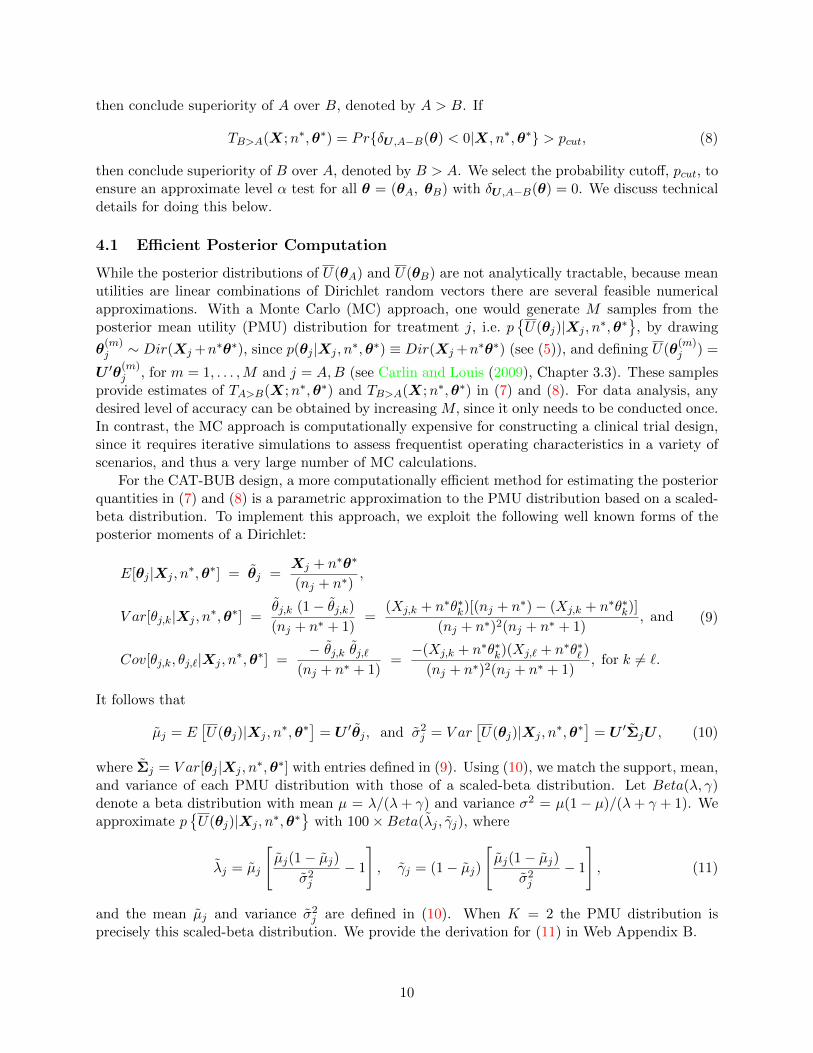
For the CAT-BUB design, a more computationally efficient method for estimating the posteriorquantities in (7) and (8) is a parametric approximation to the PMU distribution based on a scaled-beta distribution. To implement this approach, we exploit the following well known forms of theposterior moments of a Dirichlet:

E[θj |Xj , n∗,θ∗] = θj =

Xj + n∗θ∗

(nj + n∗),

V ar[θj,k|Xj , n∗,θ∗] =

θj,k (1− θj,k)(nj + n∗ + 1)

=(Xj,k + n∗θ∗k)[(nj + n∗)− (Xj,k + n∗θ∗k)]

(nj + n∗)2(nj + n∗ + 1), and

Cov[θj,k, θj,`|Xj , n∗,θ∗] =

− θj,k θj,`(nj + n∗ + 1)

=−(Xj,k + n∗θ∗k)(Xj,` + n∗θ∗` )

(nj + n∗)2(nj + n∗ + 1), for k 6= `.

(9)

It follows that

µj = E[U(θj)|Xj , n

∗,θ∗]

= U ′θj , and σ2j = V ar

[U(θj)|Xj , n

∗,θ∗]

= U ′ΣjU , (10)

where Σj = V ar[θj |Xj , n∗,θ∗] with entries defined in (9). Using (10), we match the support, mean,

and variance of each PMU distribution with those of a scaled-beta distribution. Let Beta(λ, γ)denote a beta distribution with mean µ = λ/(λ+ γ) and variance σ2 = µ(1− µ)/(λ+ γ + 1). Weapproximate p

{U(θj)|Xj , n

∗,θ∗}

with 100×Beta(λj , γj), where

λj = µj

[µj(1− µj)

σ2j

− 1

], γj = (1− µj)

[µj(1− µj)

σ2j

− 1

], (11)

and the mean µj and variance σ2j are defined in (10). When K = 2 the PMU distribution is

precisely this scaled-beta distribution. We provide the derivation for (11) in Web Appendix B.

10

Using this approximation, the posterior decision criterion is

TA>B(X;n∗,θ∗) ≈1∫

0

[1−B(x|λA, γA)]b(x|λB, γB)dx, (12)

where B(x|λ, γ) and b(x|λ, γ) denote the cdf and pdf of a Beta(λ, γ) distribution. The approxima-tion for TB>A(X;n∗,θ∗) follows by symmetry. We use adaptive quadrature via the integrate()

function in R to evaluate (12) efficiently Piessens et al. (1983). In Web Appendix B, we confirmthe validity of (12) by comparing it to the usual MC approach using simulation under a variety ofsettings. The scaled-beta approximation is 1,000 times faster than the usual MC approximationwith M = 100,000, and it works well even with very small sample sizes, such as nA = nB = 10.We will use the scaled-beta approximation for the remainder of the paper, and recommend its usein practice.

4.2 Type I Error, Power, and Sample Size

We derive an expression for the approximate power function of the CAT-BUB procedure basedon (7) and (8), and use this result to show control of type I error and to obtain a sample sizeformula. We first apply the Bayesian central limit theorem, and use the resulting posterior asymp-totic normality to obtain tractable expressions for TA>B(X;n∗,θ∗) and TB>A(X;n∗,θ∗). We willshow that the resulting approximate test statistics are tractable functions of the data, X. Wethen take the frequentist perspective, treating θ = (θA, θB) as a fixed quantity, and apply theclassical central limit theorem to derive the asymptotic sampling distributions of TA>B(X;n∗,θ∗)and TB>A(X;n∗,θ∗), and an approximate power function.

Since Xj is multinomial with parameter θj , the MLE is θj = Xj/nj and the estimated Fischer

information is njΣ−1j , where Σj has k-th diagonal entry θj,k(1− θj,k) and (k, `)-th off-diagonal entry

−θj,kθj,`, k, ` = 1, . . . ,K, j = A,B. Applying the Bayesian central limit theorem (see Gelman et al.(2014), Chapter 4)

θj |Xj , n∗,θ∗ ∼ NK(θj , n

−1j Σj), j = A,B.

Since XA and XB are independent, U ′(θA − θB)|X, n∗,θ∗ ∼ N (δU ,A−B, σ2+,n), where δU ,A−B =

U ′(θA − θB

)and σ2

+,n = U ′(ΣA/nA + ΣB/nB

)U . It follows that

TA>B(X;n∗,θ∗) ≈ Φ

(δU ,A−Bσ+,n

)and TB>A(X;n∗,θ∗) ≈ Φ

(−δU ,A−Bσ+,n

), (13)

where Φ(·) denotes the standard normal cdf. We use the notation “≈” to mean that an approxi-mation can be made arbitrarily accurate for sufficiently large sample size.

To derive an approximate power function, we treat the posterior quantities in (13) as functions ofthe data X given a fixed θ, and derive asymptotic approximations for their sampling distributions.First, the exact power function is the probability of rejecting the null for a fixed θ, i.e.

ψ(θ) = Pr {TA>B(X;n∗,θ∗) > pcut |θ}+ Pr {TB>A(X;n∗,θ∗) > pcut |θ} . (14)

Applying the classical central limit theorem, (δU ,A−B − δU ,A−B(θ))/σ+,n ∼ N (0, 1), so plugging(13) into (14) gives the approximate power function

ψ(θ)approx = Φ

[(δU ,A−B(θ)

σ+,n(θ)

)− Φ−1(pcut)

]+ Φ

[−(δU ,A−B(θ)

σ+,n(θ)

)− Φ−1(pcut)

], (15)

11

where σ+,n(θ)2 = U ′ (ΣA(θ)/nA + ΣB(θ)/nB)U . is a function of θ.The type I error is sup{ψ(θ) : δU ,A−B(θ) = 0}, and since ψ(θ)approx = 2(1− pcut) for all θ with

δU ,A−B(θ) = 0, using pcut = 1−α/2 provides an asymptotic level α test. To derive an approximatesample size formula, we set pcut = 1 − α/2 and define n = nA = nB. If desired, one could insteaddefine n = nA and nB = η×nA, where η controls the randomization ratio. For a given fixed targetalternative θ(Alt), e.g., the hypothesized outcome probabilities, we equate ψ(θ(Alt))approx = 1 − βand solve for n, which gives approximate sample size

nf

(θ(Alt), α, β

)=

[Φ−1(1− β) + Φ−1(1− α/2)

]2σ2

+(θ(Alt))

δ2U ,A−B(θ(Alt))

. (16)

We discuss elicitation of θ(Alt) in Section 5.

5 Designing a CAT-BUB Trial

In this section, we derive design parameters that control overall type I error at level α and provide1-β power for targeted alternatives, i.e., the set of treatment effects that we want to identify withthe specified power. For this computation, we distinguish between fixed sample designs with onecomparative test at the end of the trial, and group sequential designs with up to S comparativeanalyses over the course of the trial, allowing early termination with rejection of the null at eachinterim analysis. We first present guidelines for eliciting targeted alternatives, then discuss fixedsample CAT-BUB designs, followed by group sequential CAT-BUB designs. For each design setting,we provide a computational algorithm for deriving the probability cut-offs and sample size, givenα, β and the targeted alternatives.

5.1 Eliciting Targeted Alternatives

Consider a fixed sample CAT-BUB test with type I error α for all θ for which δU ,A−B(θ) = 0,and power 1 − β for a set of fixed targeted alternatives with |δU ,A−B(θ)| > 0. The approximatepower function in (15) shows that selecting pcut to control type I error for one fixed null response

probability vector, say θ(Null) =(θ

(Null)A , θ

(Null)B

)with δ

(Null)U ,A−B = 0, will control type I error for all

fixed θ with δU ,A−B(θ) = 0. In contrast, the power varies with both the targeted utility differenceand the fixed θ from which this difference arises, via σ+,n(θ). Therefore, targeted alternatives must

be elicited in the θ domain. We denote a fixed target by θ(Alt) =(θ

(Alt)A , θ

(Alt)B

)and its utility

difference by∣∣∣δ(Alt)

U ,A−B

∣∣∣ > 0.

Since it may not be intuitively obvious how to specify θ(Alt), we provide the following guidelines,which require a discussion between the statistician and the physicians. For simplicity, we will treatA as the null or standard treatment, although the algorithm works if A and B are both experimentaland considered to be symmetric. The statistician begins by eliciting an expected probability vector

corresponding to historical experience with standard therapy, say θ(Alt)A , which may be based on

the physician(s)’ experience or analysis of historical data. Given θ(Alt)A , the statistician asks the

physician(s) to specify one or more alternative probability vectors, θ(Alt,1)B , · · · ,θ(Alt,m)

B , that are

considered equally desirable improvements over θ(Alt)A . In practice, m should be reasonably small,

in the range 1 ≤ m ≤ K. Each elicited alternative θ(Alt,r)B gives standardized utility difference

s(Alt,r) = δ(Alt,r)U ,B−A/σ

(Alt,r)+ , where δ

(Alt,r)U ,B−A and σ

(Alt,r)+ are evaluated at θ(Alt,r) =

(θ

(Alt)A , θ

(Alt,r)B

)12

for r = 1, . . . ,m. For the sample size calculation in (16), one then selects the targeted alternative

θ(Alt)B giving smallest s(Alt,r), formally

θ(Alt) ={(θ

(Alt)A , θ

(Alt,r∗)B

): s(Alt,r∗) = min{s(Alt,1), . . . , s(Alt,m)}

}. (17)

This choice is conservative since it ensures the test will achieve the desired power for all elicitedθ(Alt,r).

In practice, if this computation gives a sample size that is not feasible, then the physician(s)should be asked to re-consider their set of specified alternatives. This is not unlikely, since it maynot be intuitively obvious, when specifying one or more fixed target probability vectors, how theytranslate into a required sample size. To help guide the physician(s) in this process, one should

show them the numerical values of δ(Alt,r)U ,B−A, s

(Alt,r), and θ(Alt,r)B , for r = 1, · · · ,m, possibly as a

table with m rows and three columns to facilitate comparison and interpretation. Since smaller

values of s(Alt,r) and δ(Alt,r)U ,B−A require a larger sample size to detect the corresponding θ

(Alt,r)B , this

provides a quantitative index of the relative difficulty of detecting each target, and it also identifies

the targeted alternative θ(Alt,r∗)B having the smallest s(Alt,r) that produced the sample size. If a

modified set of targets is specified, the sample size may be recomputed, with this process iteratedif desired. This may be considered a multidimensional analog of a conventional power and samplesize computation in terms of a one-dimensional parameter. If desired, the CAT-BUB test’s powerfunction computed over a set of (θA, θB) values also may be examined.

Recall the trinary outcome example where U = (UR, UN , UF )′ = (100, 60, 0)′. Given stan-

dard vector θ(Alt)A = (0.30, 0.50, 0.20)′, suppose that the three equally desirable targets θ

(Alt,1)B =

(0.40, 0.50, 0.10)′, θ(Alt,2)B = (0.50, 0.35, 0.15)′, and θ

(Alt,3)B = (0.35, 0.60, 0.05)′ are elicited. Then

s(Alt,1) = 10/45.8 = 0.218, s(Alt,2) = 11/49.2 = 0.224, and s(Alt,3) = 11/42.6 = 0.258, so we would

take θ(Alt) =(θ

(Alt)A , θ

(Alt,1)B

). If the standardized utility differences, s(Alt,r), differ substantially,

then the physician(s) may instead select the a priori most likely alternative, perhaps sacrificing

power for some alternatives as a trade-off for a smaller sample size. If the utility differences, δ(Alt,r)U ,B−A,

differ substantially, then the physician(s) may wish to reconsider the choices of equally desirabletargets, or possibly may decide to modify some entries of the numerical utility vector U .

5.2 Computational Algorithm for Fixed Sample CAT-BUB Design

Given α, β and the targeted alternative θ(Alt) defined in (17), we jointly select a sample size andcutoff pcut for a fixed sample CAT-BUB design using the following algorithm:

Step 0. Set n = nf (θ(Alt), α, β), where nf (·) is defined by (16).

Step 1. Generate G0 null datasets as follows. For g0 = 1, . . . , G0,

(i) generate X(g0)j ∼Mult

(n, θ

(Alt)A

)for j = A,B.

(ii) store X(Null,g0) =(X

(g0)A , X

(g0)B

).

(iii) calculate and storeT (Null,g0) = max

{TA>B

(X(Null,g0);n∗,θ∗

), TB>A

(X(Null,g0);n∗,θ∗

)}.

Step 2. Set pcut to the empirical (1− α)%-tile of{T (Null,1), · · · , T (Null,G0)

}.

Step 3. Generate G1 alternative datasets as follows. For g1 = 1, . . . , G1,

(i) generate X(g1)j ∼Mult

(n, θ

(Alt)j

)for j = A,B.

13

(ii) store X(Alt,g1) =(X

(g1)A , X

(g1)B

).

(iii) If δ(Alt)U ,A−B > 0, calculate and store T (Alt,g1) = TA>B

(X(Alt,g1);n∗,θ∗

).

Otherwise, calculate and store T (Alt,g1) = TB>A(X(Alt,g1);n∗,θ∗

).

Step 4. Set β = G−11

G1∑g1=1

[T (Alt,g1) ≤ pcut

], where [E] = 1 if E is true, and 0 otherwise.

Step 5. If β ∈ [β − ε, β + ε], stop and select n = n and pcut = pcut.

Otherwise, update n = n(

Φ−1(1−β)+Φ−1(pcut)

Φ−1(1−β)+Φ−1(pcut)

)2and return to Step 1.

In practice, n is rounded to its nearest integer value and pcut is rounded to its nearest largerthousandth. We use default values ε = 0.005, G0 = 50, 000 and G1 = 25, 000. Since choosing G0

and G1 is non-intuitive, detailed guidelines are given in Web Appendix C. Briefly, these defaultvalues allow us to estimate pcut accurately to three digits, and be certain that the power for θ(Alt)

at the selected n is within 2× ε = 0.01 of 1−β. The sample size adjustment in step 5 is motivatedby (16), and allows n to be increased or decreased by a magnitude proportional to the currentdiscrepancy between the estimated and desired power.

5.3 Computational Algorithm for Group Sequential CAT-BUB Design

In typical practice, RCTs require group sequential tests Jennison and Turnbull (2000). Here, wediscuss implementation of the CAT-BUB test in this context, denoting the sample sizes where ananalysis occurs by ns, s = 1, . . . , S. We take use the α-spending approach proposed by Slud andWei (1982) and extended by Lan and DeMets (1983), with an α-spending function f(ns;α, ρ, nS)= α(ns/nS)ρ suggested by Kim and DeMets (1987). The design parameter ρ ≥ 0 controls theα-spending rate, with larger values spending less α at early looks. This approach is appealing inpractice because the actual analysis schedule need not follow the planned schedule. At the firstinterim look with n1 of the planned nS samples, we calibrate the probability threshold, pcut,1, tospend f(n1;α, ρ, nS) of the overall type I error. Similarly, at s-th interim look, we calibrate pcut,sto spend f(ns;α, ρ, nS) - f(ns−1;α, ρ, nS) of the overall type I error. So if the trial reaches a finalanalysis at nS samples, the overall type I error is exactly α.

To determine a maximum sample size, nS , for a group sequential CAT-BUB design with up toS tests, power 1−β for the elicited alternative θ(Alt), we specify a complete analysis schedule usingthe proportions of nS , denoted by ts, s = 1, . . . , S. We determine nS using the following algorithm:

Step 0. Set nS = nf (θ(Alt), α, β), where nf (·) is defined by (16), and ns = ts × nS , for s =1, . . . , S − 1.

Step 1. Generate G0 null sequential datasets as follows. For g0 = 1, . . . , G0,

(i) generate X(g0)j,s ∼Mult

(ns, θ

(Alt)A

)for j = A,B and s = 1, . . . , S.

(ii) store X(Null,g0)s,+ =

(X

(g0)A,s,+, X

(g0)B,s,+

), where X

(g0)j,s,+ =

s∑m=1

X(g0)j,m

for j = A,B and s = 1, . . . , S.(iii) calculate and store, for s = 1, . . . , S,

T(Null,g0)s = max

{TA>B

(X

(Null,g0)s,+ ;n∗,θ∗

), TB>A

(X

(Null,g0)s,+ ;n∗,θ∗

)}.

Step 2. Calculate pcut,1, . . . , pcut,S as follows.

(i) Set pcut,1 to the empirical {1− f(n1;α, ρ, nS)}%-tile of{T

(Null,1)1 , . . . , T

(Null,G0)1

}.

14

(ii) Set pcut,s to the empirical [{1− f(ns;α, ρ, nS)}/{1− f(ns−1;α, ρ, nS)}]%-tile of{T

(Null,g0)s : T

(Null,g0)1 ≤ pcut,1, · · · , T (Null,g0)

s−1 ≤ pcut,s−1, g0 = 1, . . . , G0

}for s = 2, . . . , S.

Step 3. Generate G1 alternative sequential datasets as follows. For g1 = 1, . . . , G1,

(i) generate X(g1)j,s ∼Mult

(ns, θ

(Alt)j

)for j = A,B and s = 1, . . . , S.

(ii) store X(Alt,g1)s,+ =

(X

(g1)A,s,+, X

(g1)B,s,+

), where X

(g1)j,s,+ =

s∑m=1

X(g1)j,m for j = A,B and

s = 1, . . . , S.

(iii) If δ(Alt)U ,A−B > 0, calculate and store T

(Alt,g1)s = TA>B

(X

(Alt,g1)s,+ ;n∗,θ∗

), for s =

1, . . . , S.

Otherwise, calculate and store T(Alt,g1)s = TB>A

(X

(Alt,g1)s,+ ;n∗,θ∗

), for s =

1, . . . , S.

Step 4. Set β = G−11

G1∑g1=1

[T

(Alt,g1)1 ≤ pcut,1, · · · , T (Alt,g1)

S ≤ pcut,S

], where [E] = 1, if E is true,

and 0, otherwise.

Step 5. If β ∈ [β − ε, β + ε], stop and select nS = nS .

Otherwise, update nS = nS

(Φ−1(1−β)+Φ−1(pcut,S)

Φ−1(1−β)+Φ−1(pcut,S)

)2, ns = ts × nS for s = 1, . . . , S − 1, and

return to Step 1.

We use the same default values as the fixed sample algorithm, that is ε = 0.005, G0 = 50, 000 andG1 = 25, 000. Using the planned analysis schedule, we can assess the operating characteristics at avariety of alternatives. The actual analysis schedule may differ from the planned schedule, so therealized power may differ from 1−β; however, Jennison and Turnbull (2000) show that the realizedpower is quite robust to deviations from the planned analysis schedule. During an actual trial, wecan follow steps 1–2 to re-estimate pcut,s for the actual ns being used, given the previous interimanalysis sample sizes n1, . . . , ns−1 and their corresponding pcut,1, . . . , pcut,s−1 values.

6 Illustrations

In this section, we illustrate CAT-BUB tests and report results of various simulation studies com-paring both fixed sample and group sequential CAT-BUB designs with beta-binomial designs. Weinvestigate the proposed procedure in the contexts of a trinary outcome, a bivariate-binary out-come, and the CLL trial, which actually had a bivariate ordinal outcome including death. We alsoreport the results of utility sensitivity analyses.

6.1 Trinary Outcomes

6.1.1 Fixed Sample Tests

Returning to the example involving clot dissolving agents for rapid treatment of stroke with a trinaryoutcome and utility U = (100, 50, 0)′, we investigate the frequentist operating characteristics ofthe proposed CAT-BUB approach for a variety of fixed response probability vectors. We consider aCAT-BUB test with type I error α = 0.05, and power 1−β = 0.80 for targeted alternative θ(Alt) =(θ

(Alt)A , θ

(Alt)B

)= ((0.50, 0.30, 0.20)′, (0.60, 0.30, 0.10)′) with δ

(Alt)U ,B−A = 10. In this context, the

fixed sample CAT-BUB design algorithm, given in Section 5.2, gives pcut = 0.976 and n = 208.

15

Table 2: Power of a fixed sample CAT-BUB design for trinary outcome {R,N,F} versus a beta-binomial design based on “success” probability πj = θj,R, for j = A,B. In all scenarios, θA =(0.50, 0.30, 0.20)′ and nA = nB = 208. Results in the first row are based on 50,000 simulations(std.err. ≈0.001), whereas all other results are based on 25,000 simulations (std.err. <0.0032).

Scenario CAT-BUB Design Beta-Bin DesignθB δU ,B−A(θ) B > A A > B B > A A > B

1.0: (0.50, 0.30, 0.20) 0 0.025 0.025 0.025 0.025

2.1: (0.60, 0.00, 0.40) -5 0.001 0.206 0.552 0.0002.2: (0.60, 0.10, 0.30) 0 0.024 0.0252.3: (0.60, 0.20, 0.20) 5 0.246 0.0012.4: (0.60, 0.30, 0.10) 10 0.798 0.0002.5: (0.60, 0.40, 0.00) 15 0.997 0.000

3.1: (0.65, 0.05, 0.30) 2.5 0.088 0.006 0.877 0.0003.2: (0.65, 0.15, 0.20) 7.5 0.485 0.0003.3: (0.65, 0.25, 0.10) 12.5 0.936 0.0003.4: (0.65, 0.35, 0.00) 17.5 1.000 0.000

4.1: (0.70, 0.00, 0.30) 5 0.217 0.001 0.989 0.0004.2: (0.70, 0.10, 0.20) 10 0.720 0.0004.3: (0.70, 0.20, 0.10) 15 0.987 0.0004.4: (0.70, 0.30, 0.00) 20 1.000 0.000

We compare the CAT-BUB approach for trinary outcomes {R,N,F} with a Bayesian designthat follows the more common approach of combining the events N and F so that outcome may beconsidered binary, specifically R = “success,” versus N ∪F = “failure,” and compares therapies interms of the probabilities πj = Pr(Y = R | j) for j=A,B. For this design, we assume a Bayesian beta-binomial model with common beta priors πj | qj ∼ Beta(qj,1 = 0.50, qj,2 = 0.50) for j = A,B, whichhas ESS = 1. The posterior is Beta(Sj + 0.50, nj −Sj + 0.50), where Sj is the number of successesout of nj in arm j. Denoting W = (SA, nA−SA, SB, nB−SB) and q = (qA,1, qA,2, qB,1, qB,2), weuse the test statistic SA>B(W ; q) = Pr(πA > πB|W , q), which we calculate similarly to (12). Thisis the special case of the Dirichlet-multinomial model and CAT-BUB test with K = 2, since themean utility for treatment j is 100× πj , so the utility is superfluous. To ensure comparability, forthe binary test we also use n = 208, and set pcut = 0.975 to obtain a 0.05-level test when πA = πB.

Operating characteristics of the fixed sample CAT-BUB and beta-binomial tests are given inTable 2. Scenario 1.0 is the null case used to calibrate pcut for each design, so the type I error forboth designs is 0.05, with equal probabilities for concluding A > B or B > A. Scenario 2.4 is thealternative used to select a sample size that provides power 0.80, so the estimated power is in theinterval [0.80− ε, 0.80 + ε]. For Scenarios 2.1-2.5, πB is fixed at 0.60 versus πA = 0.50, so the beta-binomial design always has power 0.55, despite obvious differences between these four scenarios.For example, in Scenarios 2.1 and 2.2, the beta-binomial design fails by concluding B > A 55%of the time even though A is clinically superior or equal to B in terms of δU ,B−A(θ). In contrast,the CAT-BUB test distinguishes between these scenarios, correctly concluding A > B 21% of thetime in Scenario 2.1 and controlling type I error at 0.05 in Scenario 2.2. Scenarios 2.3-2.5 exhibitvarious tradeoffs that favor B over A in an increasing manner in terms of δU ,B−A(θ) = 5, 10, 15and the CAT-BUB test reflects this with increasing power figures 0.246, 0.798, 0.997. In particular,the CAT-BUB test has substantially more power than the beta-binomial test for the “win-win”Scenarios 2.4 and 2.5. Scenarios 3.1-3.4 and 4.1-4.4 respectively fix the probability of response

16

at 0.65 or 0.70, for which the beta-binomial test has 0.88 and 0.99 power figures. In contrast,the power of the CAT-BUB test increases as the true utility difference δU ,B−A(θ) increases, andequals or exceeds that of the beta-binomial design in “win-win” scenarios where the probability offailure is also reduced (Scenarios 3.3-3.4 and 4.3-4.4). The failure of the beta-binomial design isdue to B providing an unfavorable trade-off between the probability of response and failure versusA. Such tradeoffs cannot be identified by the naive binary outcome design, which is used verycommonly. The price of the CAT-BUB approach is potentially less power for “tradeoff” scenarioswhen the treatment redistributes probability away from N to R and/or F (Scenarios 2.3, 3.2, 4.1and 4.2). However, we feel that this price is well worth being able to distinguish between, forexample, Scenarios 2.1-2.5 in practice. Lastly, the CAT-BUB test has varying power over the set ofθ with the same utility difference. For example, Scenarios 2.3 and 4.1 have utility difference 5, yetpower figures 0.25 and 0.22, respectively. The CAT-BUB design’s power varies more substantiallywith δU ,A−B(θ) than over the set of θ with the same utility difference.

6.1.2 Sensitivity to Elicited Utilities

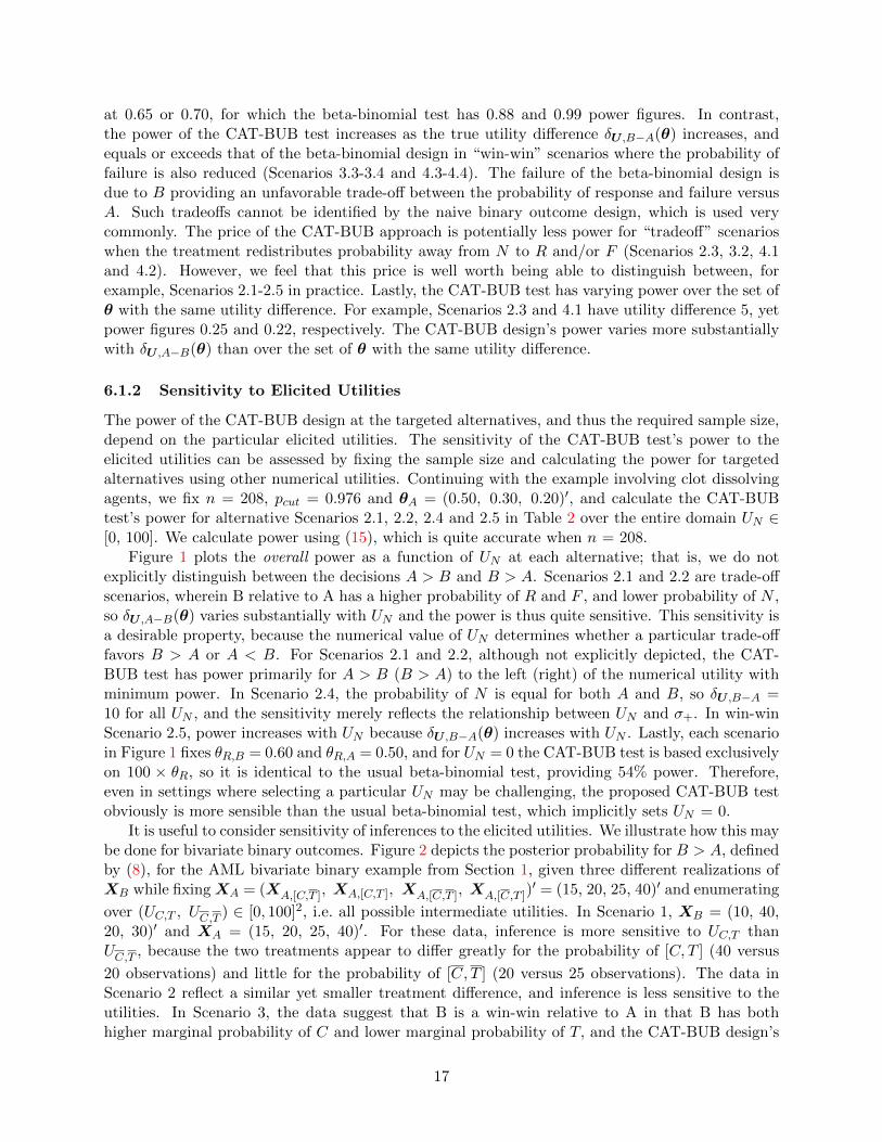
The power of the CAT-BUB design at the targeted alternatives, and thus the required sample size,depend on the particular elicited utilities. The sensitivity of the CAT-BUB test’s power to theelicited utilities can be assessed by fixing the sample size and calculating the power for targetedalternatives using other numerical utilities. Continuing with the example involving clot dissolvingagents, we fix n = 208, pcut = 0.976 and θA = (0.50, 0.30, 0.20)′, and calculate the CAT-BUBtest’s power for alternative Scenarios 2.1, 2.2, 2.4 and 2.5 in Table 2 over the entire domain UN ∈[0, 100]. We calculate power using (15), which is quite accurate when n = 208.

Figure 1 plots the overall power as a function of UN at each alternative; that is, we do notexplicitly distinguish between the decisions A > B and B > A. Scenarios 2.1 and 2.2 are trade-offscenarios, wherein B relative to A has a higher probability of R and F , and lower probability of N ,so δU ,A−B(θ) varies substantially with UN and the power is thus quite sensitive. This sensitivity isa desirable property, because the numerical value of UN determines whether a particular trade-offfavors B > A or A < B. For Scenarios 2.1 and 2.2, although not explicitly depicted, the CAT-BUB test has power primarily for A > B (B > A) to the left (right) of the numerical utility withminimum power. In Scenario 2.4, the probability of N is equal for both A and B, so δU ,B−A =10 for all UN , and the sensitivity merely reflects the relationship between UN and σ+. In win-winScenario 2.5, power increases with UN because δU ,B−A(θ) increases with UN . Lastly, each scenarioin Figure 1 fixes θR,B = 0.60 and θR,A = 0.50, and for UN = 0 the CAT-BUB test is based exclusivelyon 100 × θR, so it is identical to the usual beta-binomial test, providing 54% power. Therefore,even in settings where selecting a particular UN may be challenging, the proposed CAT-BUB testobviously is more sensible than the usual beta-binomial test, which implicitly sets UN = 0.

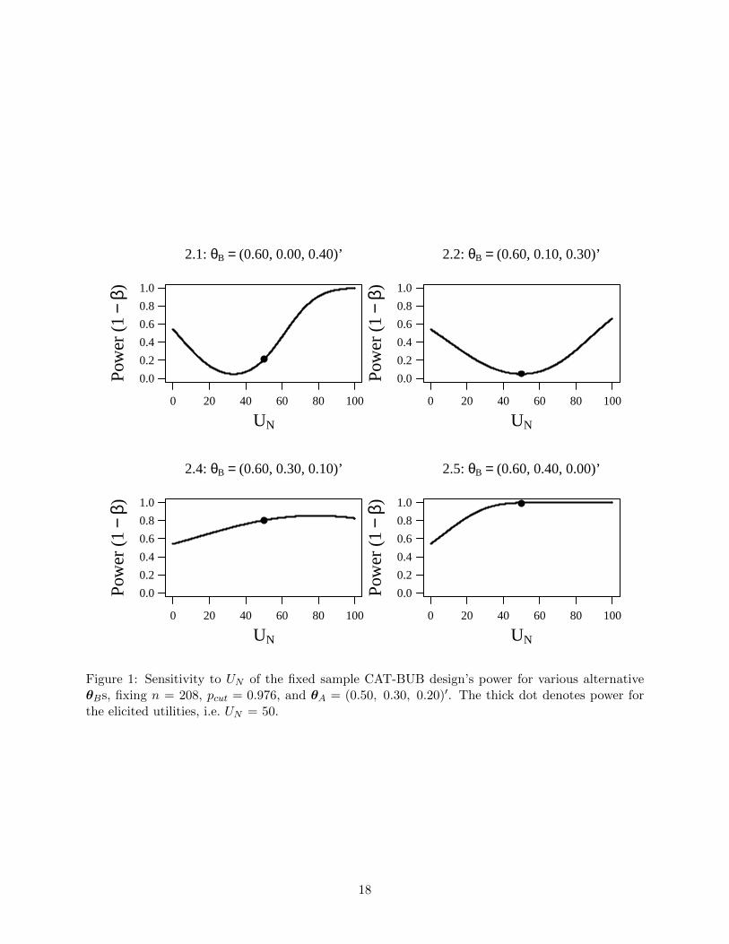
It is useful to consider sensitivity of inferences to the elicited utilities. We illustrate how this maybe done for bivariate binary outcomes. Figure 2 depicts the posterior probability for B > A, definedby (8), for the AML bivariate binary example from Section 1, given three different realizations ofXB while fixingXA = (XA,[C,T ], XA,[C,T ], XA,[C,T ], XA,[C,T ])

′ = (15, 20, 25, 40)′ and enumerating

over (UC,T , UC,T ) ∈ [0, 100]2, i.e. all possible intermediate utilities. In Scenario 1, XB = (10, 40,20, 30)′ and XA = (15, 20, 25, 40)′. For these data, inference is more sensitive to UC,T thanUC,T , because the two treatments appear to differ greatly for the probability of [C, T ] (40 versus

20 observations) and little for the probability of [C, T ] (20 versus 25 observations). The data inScenario 2 reflect a similar yet smaller treatment difference, and inference is less sensitive to theutilities. In Scenario 3, the data suggest that B is a win-win relative to A in that B has bothhigher marginal probability of C and lower marginal probability of T, and the CAT-BUB design’s

17

0 20 40 60 80 100

0.0

0.2

0.4

0.6

0.8

1.0

2.1: θB = (0.60, 0.00, 0.40)’

UN

Pow

er (

1−

β)

0 20 40 60 80 100

0.0

0.2

0.4

0.6

0.8

1.0

2.2: θB = (0.60, 0.10, 0.30)’

UN

Pow

er (

1−

β)

0 20 40 60 80 100

0.0

0.2

0.4

0.6

0.8

1.0

2.4: θB = (0.60, 0.30, 0.10)’

UN

Pow

er (

1−

β)

0 20 40 60 80 100

0.0

0.2

0.4

0.6

0.8

1.0

2.5: θB = (0.60, 0.40, 0.00)’

UN

Pow

er (

1−

β)

Figure 1: Sensitivity to UN of the fixed sample CAT-BUB design’s power for various alternativeθBs, fixing n = 208, pcut = 0.976, and θA = (0.50, 0.30, 0.20)′. The thick dot denotes power forthe elicited utilities, i.e. UN = 50.

18

UC, T

UC

, T

0.1

0.2

0

.3

0.4

0

.5

0.6

0

.7

0.8

0

.9

0.9

5

0 10 20 30 40 50 60 70 80 90 100

0102030405060708090

100

1 : XB = (10, 40, 20, 30)’

UC, T

UC

, T 0.3

0

.4

0.5

0

.6

0.7

0

.8

0.9

0 10 20 30 40 50 60 70 80 90 100

0102030405060708090

100

2 : XB = (15, 30, 20, 35)’

UC, T

UC

, T

0.8

0.9

0

.95

0.99

0 10 20 30 40 50 60 70 80 90 100

0102030405060708090

100

3 : XB = (20, 30, 25, 25)’

Figure 2: Posterior probability of B > A while varying (UC,T , UC,T ) for three different realizationsof XB and XA = (XA,[C,T ], XA,[C,T ], XA,[C,T ], XA,[C,T ])

′ = (15, 20, 25, 40)′. The thick dot

denotes our inferential result at the elicited utilities, i.e. (UC,T = 80, UC,T = 40).

inference always supports the conclusion B > A. For these data, posterior evidence supportingB > A becomes stronger as UC,T is increased.

6.1.3 Group Sequential Tests

To assess the operating characteristics of the group sequential tests, we continue with the trinaryversus binary example. We assume the analysis schedule has S = 3 equally spaced looks at t1= 0.33, t2 = 0.66 and t3 = 1. We use the same targeted alternative as the fixed sample designfor calibration, and compare the operating characteristics of the group sequential versions of theCAT-BUB design and beta-binomial design for Scenarios 1.0 and 2.1-2.5 used for the fixed samplesimulation. We applied the group sequential CAT-BUB design algorithm, given in Section 5.3, tomaintain α ≤ 0.05 with ρ = 3. This gave nS = 213, pcut,1 = 0.999, pcut,2 = 0.993 and pcut,3 =0.978. Scenarios 1.0 and 2.4 were used to jointly calibrate the planned sample size and probabilitythresholds to provide type I error of 0.05 and overall power of 0.80, respectively. For the beta-binomial design, to maintain size 0.05 we used pcut,1 = 0.999, pcut,2 = 0.992 and pcut,3 = 0.979. Weused nS = 213 for both designs to ensure comparability.

The results of the group sequential simulations are reported in Table 3. For the null Scenario 1.0,the operating characteristics of the CAT-BUB and beta-binomial designs are practically identical.Both designs have an average sample size of 212 and overall type I error of 0.05. In contrast, forScenarios 2.1-2.5, the operating characteristics of the two designs differ dramatically. The beta-binomial design does not distinguish between these scenarios because πB,R = 0.60 and πA,R = 0.50for all 5 scenarios, whereas the CAT-BUB test distinguishes between them quite well. In Scenario2.1, A is preferred over B due to an unfavorable tradeoff between R and F . The beta-binomialdesign incorrectly selects B over A 54% of the time with an average sample size of 193, whereas theCAT-BUB design correctly selects A over B 21% of the time with an average sample size of 208.In Scenario 2.2, B and A are equivalent due to the increase in response probability being canceled

19

Table 3: Power figures of a group sequential CAT-BUB design for a trinary outcome {R.N, F}versus a beta-binomial design based on “success” probabilities πj = θj,R, for j = A,B. In eachscenario, θA = (0.50, 0.30, 0.20)′, n1 = 71, n2 = 142, n3 = 213, and ρ = 3.

Scenario Specification CAT-BUB Design Beta-Binomial DesignθB δU ,B−A(θ) Ave SS B > A A > B Ave SS B > A A > B

1.0: (0.50, 0.30, 0.20) 0 211.9 0.025 0.025 211.8 0.026 0.024

2.1: (0.60, 0.00, 0.40) -5 207.7 0.001 0.214 192.8 0.541 0.0002.2: (0.60, 0.10, 0.30) 0 211.8 0.026 0.0252.3: (0.60, 0.20, 0.20) 5 206.6 0.250 0.0012.4: (0.60, 0.30, 0.10) 10 177.8 0.800 0.0002.5: (0.60, 0.40, 0.00) 15 123.8 0.998 0.000

out by the increase in failure probability. Here, the CAT-BUB design controls type I error at level0.05. Scenarios 2.3-5 have increasing magnitudes of the benefit for B over A, and the CAT-BUBdesign has increasing power for concluding B > A. As the true benefit of B over A increases, theaverage sample size of the CAT-BUB design decreases because the probability of early terminationincreases. In the most favorable Scenario 2.5, the CAT-BUB design has power 0.998 and terminatesearly nearly 95% of the time, with average sample size 124 that is 42% smaller than the plannedmaximum sample size. In contrast, the beta-binomial design has 54% power and average samplesize 193 in this case, as in all Scenarios 2.1 - 2.5, essentially because it ignores the distinctionbetween N and F.

6.2 Redesigning the CLL Trial

Returning to the CLL trial, we illustrate how to implement the CAT-BUB design in this context.We assume that the elicited numerical utilities are those in Table 1. Recall that, since we cannotelicit utilities for this trial retrospectively, as explained in Section 1 the utilities in Table 1 arespecified to be a reasonable representation of what one actually would elicit in practice. Wecompare the CAT-BUB design with a beta-binomial design based on an efficacy test, which wedenote by BB-EO. Like the actual trial, the BB-EO design defines efficacy using a binary indicatorfor CR, where the comparative test was based on targeted alternative CR probability πCR,FC =0.45 versus null πCR,F = 0.25 Flinn et al. (2007). We also compare the CAT-BUB design to analternative approach that is based on a hierarchical testing procedure. This alternative design firstcompares the probabilities of efficacy (here, CR) as the primary endpoint and, if this test fails toreject the null, then the procedure compares the probabilities of toxicity (here, severe or fatal AE)in a second test. This design, which we denote by BB-ET, assumes independent beta-binomialmodels for the two outcomes. Based on this hierarchical testing procedure, the BB-ET designrecommends a treatment if it is found to have either better efficacy or toxicity compared to theother treatment.

Because the actual CLL trial outcome is bivariate ordinal plus death, to implement the CAT-BUB design, a practical approach for eliciting the targeted alternative(s) is as follows. First, askthe physicians to hypothesize the marginal probabilities of the AE levels, {Min, Mod, Sev, Fatal},in each treatment group. Denote these probabilities by

θj,T = (θj,Min, θj,Mod, θj,Sev, θj,Fatal), where θj,Min + θj,Mod + θj,Sev + θj,Fatal = 1, j = F, FC.

Next, ask the physicians to hypothesize probabilities of the clinical response events, {CR, PR, SD,

20

Table 4: Response probabilities for the scenarios considered in our CLL trial simulation study.Toxicity probabilities correspond to {Min, Mod, Sev, Fatal}, and efficacy probabilities correspondto {CR, PR, SD, PD}, given that the patient is alive.

Scenarios Abbreviation Response Probabilities

All NA θF,T = (0.67, 0.25, 0.05, 0.03)1.0, 2.0, 3.0, 4.0 = θFC,T = (0.67, 0.25, 0.05, 0.03)1.1, 2.1, 3.1, 4.1 > θFC,T = (0.44, 0.40, 0.10, 0.06)1.2, 2.2, 3.2, 4.2 >> θFC,T = (0.26, 0.45, 0.20, 0.09)

All NA θF,E = (0.25, 0.35, 0.20, 0.20)1.0, 1.1, 1.2 = θFC,E = (0.25, 0.35, 0.20, 0.20)2.0, 2.1, 2.2 > θFC,E = (0.35, 0.35, 0.15, 0.15)3.0, 3.1, 3.2 >> θFC,E = (0.45, 0.35, 0.10, 0.10)4.0, 4.1, 4.2 >>> θFC,E = (0.60, 0.30, 0.05, 0.05)

PD}, conditional on being alive. Denote these conditional probabilities by

θj,E = (θj,CR, θj,PR, θj,SD, θj,PD), where θj,CR + θj,PR + θj,SD + θj,PD = 1, j = F, FC.

Assuming independence for simplicity, set θ(Alt)j,Fatal = θj,Fatal and θ

(Alt)j,k,` = θj,kθj,` for j = F, FC,

k = {Min,Mod, Sev}, and ` = {CR,PR, SD,PD}. We assume that the targeted alternativearises from θF,T = θFC,T = (0.67, 0.25, 0.05, 0.03), i.e., FC and F have equivalent toxicity, andθF,E = (0.25, 0.35, 0.20, 0.20) versus θFC,E = (0.45, 0.35, 0.10, 0.10), i.e., FC compared to F hashigher efficacy. This alternative maintains similar marginal CR probabilities πCR,FC = 0.4365versus πCR,F = 0.2425 specified for the actual trial design, and it results in a large mean utility

difference δ(Alt)U ,FC−F = 13.5 for the utilities given in Table 1. Specifying n∗ = 1 and θ∗ = θF for the

Dirichlet priors, a fixed sample CAT-BUB test requires slightly more patients than a beta-binomialtest to achieve 90% power, nF = nFC = 127 versus 120. To ensure comparability, we determinethe power figures for all three designs using the larger sample size 128. We compare the designs for12 scenarios covering a wide range of different possibilities. The response probabilities for F andFC in each scenario are reported in Table 4. These probabilities for F are fixed at the targetedalternative values throughout, whereas the probabilities for FC vary with the combinations ofthe ordinal efficacy and toxicity outcomes. For each outcome, we characterize these numericalprobability vector pairs nominally as being “equivalent” (=), or having “moderate” (>), “large”(>>), or “very large” (>>>) differences.

The results of our simulation reported in Table 5 show that, in general, the CAT-BUB design issensitive to efficacy-toxicity tradeoffs characterized by the utilities, while the beta-binomial designwith an efficacy test (BB-EO) is not. In contrast, if there is low power for detecting an efficacydifference between the two treatments, then the hierarchical beta-binomial design (BB-ET) is sen-sitive to toxicity, otherwise it is not. Because the BB-ET design is based on two tests, rather thanone test like the BB-EO design, it requires a more stringent cut-off to control the type I error,and thus has lower power compared to the BB-EO design for selecting the treatment with supe-rior efficacy, which is FC in all the scenarios we considered. Scenario 1.0 is the null, i.e., θFC =(θFC,E ,θFC,T ) ≡ (θF,E ,θF,T ) = θF , and the cut-off for all three designs was calibrated to controltype I error at the α = 0.05-level, where F and FC are selected with the same 0.025 probabilities.In Scenarios 1.1 and 1.2, FC has equivalent efficacy with moderate and high toxicity, respectively,and both the CAT-BUB design and the BB-ET design are increasingly likely to select F , whereasthe BB-EO design is unable to distinguish between these clinically very different scenarios since it

21

Table 5: Power figures for the CLL trial based on the CAT-BUB design, the beta-binomial designwith an efficacy test only (BB-EO), and the hierarchical beta-binomial design with an efficacytest followed by a toxicity test (BB-ET). Comparisons of θFC,E vs θF,E and θFC,T vs θF,T arecharacterized as being “equivalent” (=), or having “moderate” (>), “large” (>>), or “very large”(>>>) differences.

Scenario Probability of Final ConclusionBeta-Binomial Designs

Efficacy Toxicity CAT-BUB Design Efficacy Only Efficacy then ToxicityFC vs F FC vs F δU,FC−F FC > F F > FC FC > F F > FC FC > F F > FC

1.0: = = 0.0 0.025 0.025 0.026 0.024 0.024 0.0251.1: = > -5.2 0.001 0.222 0.019 0.035 0.007 0.3881.2: = >> -11.9 0.000 0.782 0.012 0.047 0.005 0.982

2.0: > = 6.8 0.352 0.000 0.402 0.000 0.289 0.0102.1: > > 1.1 0.041 0.012 0.331 0.000 0.226 0.3082.2: > >> -6.5 0.000 0.314 0.278 0.000 0.173 0.818

3.0: >> = 13.5 0.903 0.000 0.910 0.000 0.846 0.0023.1: >> > 7.3 0.397 0.000 0.873 0.000 0.778 0.0973.2: >> >> -1.1 0.041 0.015 0.816 0.000 0.716 0.281

4.0: >>> = 21.0 1.000 0.000 1.000 0.000 1.000 0.0004.1: >>> > 14.2 0.917 0.000 1.000 0.000 0.999 0.0014.2: >>> >> 5.0 0.201 0.001 0.999 0.000 0.997 0.003

ignores toxicity. The BB-ET design is more likely to correctly select F than the CAT-BUB design,0.39 versus 0.22 and 0.98 versus 0.78, respectively. In Scenario 2.0, FC has a moderate efficacyadvantage with equivalent toxicity, and the BB-EO, CAT-BUB, and BB-ET designs select FCwith probabilities 0.40, 0.35, and 0.29, respectively. In Scenario 2.1, FC has a moderate efficacyadvantage and toxicity disadvantage, where this tradeoff that slightly favors FC for the assumedutilities. The CAT-BUB design is unlikely to select either treatment, whereas the BB-EO designselects FC with probability 0.33, and the BB-ET design selects FC and F with probabilities 0.23and 0.31, respectively. In Scenario 2.2, because the toxicity disadvantage for FC increases, thetradeoff moderately favors F for the assumed utilities. The CAT-BUB design selects F with higherprobability 0.31 and does not select FC, whereas the BB-EO design selects FC with probability0.28 and does not select F , and the BB-ET design selects F with probabilities 0.82 and FC withprobability 0.17. Scenario 3.0 is the targeted alternative, which is a case where FC has higherefficacy and equivalent toxicity compared to F . In this ideal case, the CAT-BUB design has 90%power compared to 91% power for the BB-EO design and 85% for the BB-ET design. Scenarios3.1, 3.2, 4.1, and 4.2 are tradeoff settings where FC has an a large or very large efficacy advantage,and either a moderate or large toxicity disadvantage. In these cases, the CAT-BUB design selectstreatments with probabilities that are sensitive to the assumed utilities, whereas the beta-binomialdesigns consistently select FC with high probability, regardless of the toxicity burden of FC.

Scenarios 1.2, 2.2, and 3.2 show very undesirable potential consequences of using the BB-EO design, which completely ignores toxicity. The BB-EO design based on the probability ofCR treats Scenario 1.2 like a null case since πCR,FC = 0.2275 versus πCR,F = 0.2425, while infact the two pairs of toxicity probability vectors θFC and θF are very different, with θFC,T =(0.26, 0.45, 0.20, 0.09) versus θF,T = (0.67, 0.25, 0.05, 0.03), so that FC has a much lower minortoxicity probability but much higher moderate, severe, and fatal AE probabilities compared to F .The CAT-BUB design recognizes this, concluding that F > FC with power 0.78 compared to 0.05for the BB-EO design. Scenario 2.2 is an intermediate case, since FC has moderate efficacy withθFC,E = (0.35, 0.35, 0.15, 0.15) versus θF,E = (0.25, 0.35, 0.20, 0.20) but also high toxicity, with

22

θFC,T = (0.26, 0.45, 0.20, 0.09) versus θF,T = (0.67, 0.25, 0.05, 0.03). The BB-EO design detectsthe 0.3185 − 0.2425 = 0.076 difference in CR probabilities in favor of FC with power 0.28, butsince the probability of severe toxicity or death is 0.29 with FC versus 0.08 with F , the CAT-BUB design concludes F is superior to FC with power 0.314 and never concludes that FC issuperior to F . In Scenario 3.2, FC has a large efficacy advantage but also high toxicity burden,with θFC,E = (0.45, 0.35, 0.10, 0.10) versus θF,E = (0.25, 0.35, 0.20, 0.20) but, as in Scenario 2.2,θFC,T = (0.26, 0.45, 0.20, 0.09) versus θF,T = (0.67, 0.25, 0.05, 0.03). The BB-EO design has power0.82 of concluding that FC is superior to F , whereas the CAT-BUB design recognizes both the muchbetter efficacy and much worse toxicity with FC compared to F , and based on the assumed utilitiesdoes not recommend either treatment over the other with probability 1 − (0.041 + 0.015) = 0.94.Scenario 4.2 shows that the BB-TE design can have a similar undesirable behavior as the BB-EOdesign. If the efficacy advantage of FC is very large, because the efficacy test will detect a differencewith high probability, the BB-TE design effectively ignores toxicity, since the toxicity test is unlikelyto be applied. In Scenarios 2.1 and 3.2, which have less extreme tradeoffs than Scenario 4.2, theBB-TE design is likely to recommend a particular treatment, despite that neither treatment maybe strongly preferred under the assumed utilities. For example, in Scenario 3.2, the BB-TE designrecommends FC and F with probabilities 0.72 and 0.28, respectively, and thus recommends eithertreatment with probability 0.99. Lastly, the BB-TE design has lower power than the CAT-BUBdesign for the targeted alternative in the CLL trial, i.e., Scenario 3.0.

There are several key points in these comparisons. First, basing a test on the probability ofCR is equivalent to using a degenerate utility-based test that assigns utilities 100 to CR and 0to its complement, while completely ignoring toxicity. An elaboration of this that accounts forthe ordinal categories of efficacy is the two-sample test of Whitehead (1993), although this teststill suffers from the fact that it ignores toxicity. Considering Scenarios 3.0, 3.1, and 3.2 togethershows how the CAT-BUB design adjusts its conclusions depending on the varying θFC,T vectors,essentially agreeing with the BB-EO design when toxicity is equivalent but very likely reachingthe opposite conclusion when FC has much higher toxicity than F . The same pattern can beseen when considering Scenarios 4.0, 4.1, and 4.2 together. This also illustrates the benefits fromconsidering the ordinal level of each outcome rather than dichotomizing it, since the probabilitiesof concluding that FC is superior to F vary from 1 to 0.20 as the probabilities of the levels of eachoutcome change across scenarios. In practice, if a conventional design based on efficacy alone isused one might hope that, in such cases, at some point during actual trial conduct someone wouldnotice an excessively higher toxicity rate in one arm compared to the other, and ask the PrincipalInvestigator or Institutional Review Board to halt accrual to the trial. Hope is not a strategy,however. Moreover, if in fact a trial designed based on efficacy alone will be stopped due to sucha toxicity difference, then the nominal size and power of the design are incorrect, and in fact theyare conditional on the assumption that there will be no difference in toxicity sufficiently large thatit would cause the trial to be stopped early. All of these concerns are taken care of automaticallyby the group sequential CAT-BUB test’s structure. For the group sequential design of the CLLtrial (see Web Supplement), its interim decision rules will stop the trial early with high probabilitywhen there is a large difference in terms of either efficacy or toxicity, as quantified by the jointutilities of the elementary (efficacy, toxicity) outcomes.

The utilities in Table 1 used for the CAT-BUB re-design of the CLL trial emphasize bothavoiding severe toxicity or death and achieving good clinical response by specifying the relativeutility parameters (Section 2) to be ζ1 = 0.1 and ζ2 = 0.2 near zero, respectively. To assessthe CAT-BUB design’s sensitivity to the utilities, we also considered the two alternative utilitiesgiven in Table 6. One alternative places greater importance on achieving better efficacy, and theother places greater importance on achieving lower toxicity. We obtained the first (second) set of

23

Table 6: Three alternative utilities for the CLL trial’s outcomes.

Level of WorstAdverse Event Clinical Response Death

Original Utilities from Table 1CR PR SD PD

Minimal 100 84 35 19Moderate 93 77 29 14 0Severe 28 24 14 10

Utilities Giving Better Efficacy Higher Value

Minimal 100 84 35 19Moderate 98 81 31 14 0Severe 82 68 24 10

Utilities Giving Lower Toxicity Higher Value

Minimal 100 93 71 64Moderate 93 81 44 32 0Severe 28 24 14 10

Table 7: Power figures for the CLL trial based on a fixed sample CAT-BUB design using twoalternative sets of numerical utilities that place greater importance on either improving efficacy orreducing toxicity, compared to the original utilities.

Alternative Utility Giving Alternative Utility GivingScenario Efficacy Higher Value Lower Toxicity Higher Value

Efficacy Toxicity δU ,FC−F FC > F F > FC δU ,FC−F FC > F F > FC

1.0: = = 0.0 0.025 0.025 0.0 0.024 0.0261.1: = > -3.2 0.003 0.100 -8.4 0.000 0.9311.2: = >> -6.7 0.000 0.287 -18.3 0.000 1.000

2.0: > = 7.1 0.349 0.000 3.6 0.365 0.0002.1: > > 3.7 0.122 0.003 -4.6 0.000 0.4702.2: > >> -0.1 0.026 0.025 -14.6 0.000 1.000

3.0: >> = 14.2 0.897 0.000 7.3 0.902 0.0003.1: >> > 10.6 0.647 0.000 -0.8 0.011 0.0493.2: >> >> 6.5 0.288 0.007 -11.0 0.000 0.986

4.0: >>> = 22.1 0.999 0.000 11.3 0.999 0.0004.1: >>> > 18.2 0.985 0.000 3.4 0.290 0.0004.2: >>> >> 13.8 0.859 0.000 -7.0 0.000 0.748

24

alternative utilities by changing ζ2 from 0.20 to 0.80 (ζ1 from 0.10 to 0.60), while retaining all otherindirect elicitation parameter values as detailed in Section 2. For the first alternative, the utilitiesof moderate or severe toxicity for CR or PR levels of efficacy are substantially increased from theoriginal utility, for example, U(CR,Sev) is increased from 28 to 82. For the second alternative, theutilities of minimal or moderate toxicity for SD or PD levels of efficacy are substantially increasedfrom the original utility, for example, U(SD,Min) is increased from 35 to 71. The required samplesizes for the two alternative utilities are nF = nFC = 110 and 271, respectively, which is in contrastto nF = nFC = 127 for the elicited numerical utilities. The CAT-BUB design based on the utilitiesthat place greater importance on higher efficacy thus requires a smaller sample size to achieve90% power for detecting the targeted alternative compared with the beta-binomial design that wasused for the actual trial. The numerical utilities that place greater importance on higher efficacy(lower toxicity) provide more (less) power for detecting the targeted alternative, which has a largetreatment difference for the marginal probabilities of clinical response and zero difference for AEprobabilities.

Table 7 reports the power figures for the same scenarios as in Table 5 for the CAT-BUB designbased on the two alternative utilities with the above sample sizes. These power figures illustrate thatthe numerical utilities affect the power of detecting specific treatment differences and determinewhich therapy is preferred for tradeoff scenarios. Scenario 4.2 is an extreme tradeoff example,wherein FC has very high efficacy and high toxicity compared to F . As shown by the mean utilitydifference and power figures, this tradeoff slightly favors FC under the original utility function,whereas FC is strongly favored under the alternative utilities that place greater importance onefficacy, and conversely, under the alternative utilities that place greater importance on lowertoxicity. The dependence of the proposed CAT-BUB design on the numerical utilities underscoresthe importance of eliciting values that actually reflect the clinical desirabilities of each patientresponse.

6.3 Additional Illustrations

In Section 1, we introduced several categorical outcome structures, including trinary, bivariatebinary, bivariate binary plus death, ordinal, and bivariate ordinal. The computational algorithmsgiven previously readily accommodate all of these cases. In Web Appendix D, we provide detailedillustrations of both fixed sample and group sequential CAT-BUB designs for a bivariate binaryoutcome, and for a bivariate ordinal outcome having 16 = 4×4 elementary events. We also includea group sequential CAT-BUB re-design of the CLL trial.

7 Discussion

Because clinical trial conduct must accommodate medical practice, a trial design should accountformally for risk-benefit tradeoffs between all clinically relevant outcomes. The utility-based teststhat we have proposed provide a practical approach for comparing treatments based on categoricaloutcomes in a RCT. We have provided both fixed sample and group sequential procedures, com-putational algorithms to derive design parameters, and freely-available user-friendly software. TheCAT-BUB test directly addresses the problem of comparing treatments for all clinically relevantdifferences. The method deals with the problem of deciding whether one therapy is clinically su-perior to another based on its outcome probability vector by exploiting the elicited utilities of theelementary outcomes to reduce the multidimensional outcome to a one dimensional mean utility.This is used to construct comparative tests. The elicited utilities provide a rigorous framework fortreatment comparison that makes explicit any subjective tradeoffs between outcomes.

25

We have demonstrated that designs based on a single binary outcome for efficacy often areunsafe, and do not reflect medical practice. Because safety is never a secondary concern in anyclinical trial, conventional designs only based on an efficacy test presumably rely on informal stop-ping criteria for safety, which makes it difficult to determine operating characteristics. We alsohave demonstrated that designs based on a hierarchical testing procedure may be unsafe in sce-narios where one treatment is more efficacious but also is more toxic than the other drug. Thesedesigns also do not reflect medical practice. If an efficacy difference is detected, it is naive to believethat the toxicity profiles of the available treatment options will not be considered by physicianswhen deciding which treatment is actually clinically preferable. In the proposed method, we haveprovided a practical tool to explicitly account for the tradeoffs between disparate outcomes thatphysicians routinely assess, and thus for designing RCTs that better reflect medical practice.

Supplementary Materials

The Web Appendices referenced in Sections 2, 4, 5, and 6 are available with this paper at the jour-nal’s website. An example spreadsheet mentioned in Section 2 for utility elicitation in the contextof the CLL example, and a suite of R functions for implementing the computational algorithms inSections 5.2 and 5.3, along with annotated example R programs for replicating each illustration areavailable at:

https://biostatistics.mdanderson.org/SoftwareDownload/

References

Brook, R. H., M. R. Chassin, A. Fink, D. H. Solomon, J. Kosecoff, and R. E. Park (1986, 1). Amethod for the detailed assessment of the appropriateness of medical technologies. InternationalJournal of Technology Assessment in Health Care 2, 53–63.

Carlin, B. P. and T. A. Louis (2009). Bayesian Methods for Data Analysis, 3rd edition. Boca-Raton,FL: Chapman & Hall/CRC Press.

Cheson, B., J. Bennett, M. Grever, N. Kay, M. Keating, S. O’Brien, and K. Rai (1996). NationalCancer Institute-Sponsored Working Group guidelines for chronic lymphocytic leukemia: revisedguidelines for diagnosis and treatment. Blood 87 (12), 4990–4997.

Dalkey, N. C. (1969). The Delphi Method: An Experimental Study of Group Opinion. Santa Monica,CA: RAND Corporation.

Eisenhauer, E., P. Therasse, J. Bogaerts, L. Schwartz, D. Sargent, R. Ford, J. Dancey, S. Arbuck,S. Gwyther, M. Mooney, L. Rubinstein, L. Shankar, L. Dodd, R. Kaplan, D. Lacombe, andJ. Verweij (2009). New response evaluation criteria in solid tumours: Revised {RECIST} guide-line (version 1.1). European Journal of Cancer 45 (2), 228 – 247. Response assessment in solidtumours (RECIST): Version 1.1 and supporting papers.

Flinn, I. W., D. S. Neuberg, M. R. Grever, G. W. Dewald, J. M. Bennett, E. M. Paietta, M. A.Hussein, F. R. Appelbaum, R. A. Larson, D. F. Moore, and M. S. Tallman (2007). Phase IIItrial of fludarabine plus cyclophosphamide compared with fludarabine for patients with previ-ously untreated chronic lymphocytic leukemia: US Intergroup Trial E2997. Journal of ClinicalOncology 25 (7), 793–798.

26

Freedman, L., G. Anderson, V. Kipnis, R. Prentice, C. Wang, J. Rossouw, J. Wittes, and D. DeMets(1996). Approaches to monitoring the results of long-term disease prevention trials: Examplesfrom the Women’s Health Initiative. Controlled Clinical Trials 17 (6), 509 – 525.

Gelman, A., J. B. Carlin, H. S. Stern, D. B. Dunson, A. Vehtari, and D. B. Rubin (2014). BayesianData Analysis, 3rd Edition. Boca-Raton, FL: Chapman & Hall/CRC Press.

Hotelling, H. (1931). The economics of exhaustible resources. Journal of Political Economy 39 (2),pp. 137–175.

Ibrahim, J. G. and M.-H. Chen (2000, 02). Power prior distributions for regression models. Statist.Sci. 15 (1), 46–60.

Jennison, C. and B. W. Turnbull (2000). Group Sequential Methods Applications to Clinical Trials.Boca-Raton, FL: Chapman & Hall/CRC Press.

Kim, K. and D. L. DeMets (1987). Design and analysis of group sequential tests based on the typeI error spending rate function. Biometrika 74 (1), 149–154.

Lan, K. K. G. and D. L. DeMets (1983). Discrete sequential boundaries for clinical trials.Biometrika 70 (3), pp. 659–663.

Murray, T., B. Hobbs, and B. Carlin (2015). Combining nonexchangeable functional or survivaldata sources in oncology using generalized mixture commensurate priors. In Press: Annals ofApplied Statistics.

Piessens, R., E. D. Doncker-Kapenga, and C. W. Uberhuber (1983). QUADPACK: a subroutinepackage for automatic integration. Springer.

Pocock, S. J. (1997). Clinical trials with multiple outcomes: A statistical perspective on their design,analysis, and interpretation. Controlled Clinical Trials 18 (6), 530 – 545. Eighth InternationalSymposium on Long-Term Clinical Trials.

Sankoh, A. J., R. B. D’Agostino, and M. F. Huque (2003). Efficacy endpoint selection and multi-plicity adjustment methods in clinical trials with inherent multiple endpoint issues. Statistics inMedicine 22 (20), 3133–3150.

Slud, E. and L. J. Wei (1982). Two-sample repeated significance tests based on the modifiedwilcoxon statistic. Journal of the American Statistical Association 77 (380), pp. 862–868.

Whitehead, J. (1993). Sample size calculations for ordered categorical data. Statistics inMedicine 12 (24), 2257–2271.

27

Web-based Supplement for “Utility-Based Designs for

Randomized Comparative Trials with Categorical

Outcomes”

Thomas A. Murray1,∗, Peter F. Thall1,† and Ying Yuan1,‡

1Department of Biostatistics, The University of Texas MD Anderson Cancer Center∗TAMurray@MDAnderson.org, †Rex@MDAnderson.org, ‡YYuan@MDAnderson.org

April 26, 2016

Outline

In Web Appendix A, we provide the generalization of the indirect utility elicitation strategy de-scribed in Section 2 for a K × L (plus death) bivariate ordinal outcome. In Web Appendix B,we provide the derivation for the moment matching technique used in Section 4 to implement ourscaled-beta approximation of the PMU distribution, and we confirm the validity of this approxi-mation using a numerical comparison with the usual MC approach and a normal approximationin a variety of settings. In Web Appendix C, we provide guidelines for selecting the Monte Carlosample sizes used in the computational algorithms defined in Section 5. In Web Appendix D, wepresent the detailed illustrations referenced in Section 6 for implementing the proposed CAT-BUBprocedures with bivariate binary and bivariate ordinal outcomes.

Web Appendix A: Generalization of the Indirect Utility ElicitationStrategy

Suppose the clinically relevant outcome is bivariate ordinal (plus death), where there are K × L(+ 1) possible elementary responses. Without loss of generality, we partially order the elementaryevents such that U(1, 1) = 100, U(1, `) ≥ U(2, `) ≥ · · · ≥ U(K, `) ≥ U(D) = 0, and U(k, 1) ≥· · · ≥ U(k, L) ≥ U(D) = 0, for k = 1, . . . ,K and ` = 1, . . . , L. To implement the indirect utilityelicitation strategy described in Section 2, the statistician would create a spreadsheet with thefollowing sub-tables for the physician(s) to fill in,

1

(A)(1, 1) (K,L) D

100 ν 0(B)

1 L

1 100 100× ζ1

K 100× ζ2 0

(C1)(1, 1) (1, 2) · · · (1, `) · · · (1, L− 1) (1, L)

100 100× φ1,1 · · · 100× φ1,`−1 · · · 100× φ1,L−2 0

(C2)(K, 1) (K, 2) · · · (K, `) · · · (K,L− 1) (K,L)

100 100× φ2,1 · · · 100× φ2,`−1 · · · 100× φ2,L−2 0

(D1)(1, 1) (2, 1) · · · (k, 1) · · · (K − 1, 1) (K, 1)

100 100× ξ1,1 · · · 100× ξk−1,1 · · · 100× ξK−2,1 0

(D2)(1, L) (2, L) · · · (k, L) · · · (K − 1, L) (K,L)

100 100× ξ1,2 · · · 100× ξk−1,2 · · · 100× ξK−2,2 0

If death is not included as a potential patient response, sub-table (A) will be omitted. If L = 2,sub-tables (C1) and (C2) will be omitted. Similarly, if K = 2, sub-tables (D1) and (D2) will beomitted. The numerical utilities that are induced by the entries in the above sub-tables can bedetermined sequentially as follows,

U(1, 1) = 100, If D, then U(D) = 0 and U(K,L) = ν, otherwise, U(K,L) = 0,

U(1, L) = ζ1[U(1, 1)− U(K,L)] + U(K,L),

U(K, 1) = ζ2[U(1, 1)− U(K,L)] + U(K,L),

U(1, `+ 1) = φ1,`[U(1, 1)− U(1, L)] + U(1, L) and

U(K, `+ 1) = φ2,`[U(K, 1)− U(K,L)] + U(K,L) for ` = 1, . . . , L− 2,

U(k + 1, 1) = ξk,1[U(1, 1)− U(K, 1)] + U(K, 1) and

U(k + 1, L) = ξk,2[U(1, L)− U(K,L)] + U(K,L) for k = 1, . . . ,K − 2, and

U(k + 1, `+ 1) =

[ξk,2(φ1,` − φ2,`) + φ2,`

1− (ξk,1 − ξk,2)(φ1,` − φ2,`)

][U(k + 1, 1)− U(k + 1, L)] + U(k + 1, L),

for k = 1, . . . ,K − 2, and ` = 1, . . . , L− 2.

The above induced numerical utilities, aside from those in the final line, i.e., U(k + 1, `+ 1), arisestraightforwardly from the below identities,

ν = [U(1, 1)− U(K,L)]/[U(K,L)− U(D)],

ζ1 = [U(1, 1)− U(1, L)]/[U(1, L)− U(K,L)],

ζ2 = [U(1, 1)− U(K, 1)]/[U(K, 1)− U(K,L)],

φ1,` = [U(1, `+ 1)− U(1, L)]/[U(1, 1)− U(1, L)] and

φ2,` = [U(K, `+ 1)− U(K,L)]/[U(K, 1)− U(K,L)] for ` = 1, . . . , L− 2,

ξk,1 = [U(k + 1, 1)− U(K, 1)]/[U(1, 1)− U(K, 1)] and

ξk,2 = [U(k + 1, L)− U(K,L)]/[U(1, L)− U(K,L)] for k = 1, . . . ,K − 2.

Using linear interpolation, the remaining numerical utilities, i.e., U(k + 1, ` + 1), arise from theidentities,

U(k + 1, `+ 1) = ηk,`[U(k + 1, 1)− U(k + 1, L)] + U(k + 1, L),

ηk,` = η′k,`[φ1,` − φ2,`] + φ2,`, and

η′k,` = ηk,`[ξk,1 − ξk,2] + ξk,2.

2

Therefore, as desired,

ηk,` = [ξk,2(φ1,` − φ2,`) + φ2,`]/[1− (ξk,1 − ξk,2)(φ1,` − φ2,`)],

for k = 1, . . . ,K − 2, and ` = 1, . . . , L− 2.

Web Appendix B: Moment Matching and Validation for the Scaled-Beta Posterior Approximation

We derive the moment matching technique used for the scaled-beta approximation of the posteriordistribution for mean utility. If X ∼ Beta(λ, γ), where µ = E[X] = λ

λ+γ and σ2 = V ar[X] =λγ

(λ+γ)2(λ+γ+1), then γ = λ(1−µ)

µ , λ + γ = λµ , and therefore σ2 = µ2(1−µ)

λ+µ . Solving the last identity

for λ, we have the first identity defined by equation (11) in the paper, i.e.

λ = µ

(µ(1− µ)

σ2− 1

).

Plugging this result into the identity γ = λ(1−µ)µ , we have the second identity defined by equation

(11) in the paper, i.e.

γ = (1− µ)

(µ(1− µ)

σ2− 1

).

We address the validation of the scaled-beta posterior approximation with two inquiries. In thefirst, we investigate how well the scaled-beta distribution approximates the actual PMU distribu-tion, using the MC approach with M=1,000,000 as the gold standard, given various realizations ofX. In the second, we investigate the frequentist properties of the proposed CAT-BUB comparativetesting procedure using the posterior quantities defined by equations (7) and (8) in the paper basedon the scaled-beta approximation versus that based on the usual MC approach and the normalapproximation defined by equation (13).

For our first assessment, we consider a single treatment with a trinary outcome and utilitiesU = (100, 50, 0)′. For Scenario A we assume the observed data are X = n × (0.50, 0.30 , 0.20);whereas, for Scenario B we assume X = n × (0.10, 0.10, 0.80). For both scenarios, we fix nequal to each of the values in the set {10, 25, 50, 100} and use the usual MC approach withM=1,000,000 to estimate the actual PMU distribution. We then compare this precise estimate ofthe PMU distribution with the proposed scaled-beta approximation. The results of this assessmentare displayed in Figure 1. As evidenced by Figure 1, the scaled-beta approximation is nearlyindistinguishable from MC estimate even in small sample sizes (e.g. n=10 and 25) and non-negligibleposterior density near the boundaries of the PMU distribution’s domain (i.e. Scenario B).

For our second assessment, we continue with the example involving clot dissolving agents forrapid treatment of stroke with a trinary outcome and utility U = (100, 50, 0)′. We investigatethe power of the CAT-BUB approach for a variety of fixed response probability vectors. Weconsider one CAT-BUB test based on the usual MC approach with M=100,000, one based onthe proposed scaled-beta approximation, and one based on a normal approximation matching thePMU distribution’s mean and variance using the results from equation (10) in the paper. Usingsimulation, we tuned the threshold pcut for each Bayesian test to control type I error at 0.05 underpoint null hypothesis θA = θB = (0.50, 0.30, 0.20)′ with 100 observations in each therapy arm.

The results of this simulation are reported in Table 1, and they show that scaled-beta approxi-mation is nearly indistinguishable from the MC approach, while the normal approximation differs

3

0 20 40 60 80 100

0.00

0.05

0.10

0.15

n = 10

U(θ)

p[U

(θ) |

X] Scenario A

Scenario BMonte CarloScaled Beta

0 20 40 60 80 100

0.00

0.05

0.10

0.15

n = 25

U(θ)

p[U

(θ) |

X]

0 20 40 60 80 100

0.00

0.05

0.10

0.15

n = 50

U(θ)

p[U

(θ) |

X]

0 20 40 60 80 100

0.00

0.05

0.10

0.15

n = 100

U(θ)

p[U

(θ) |

X]

Figure 1: Numerical assessment of the proposed beta approximation for the posterior distributionof mean utility.

4

Table 1: Simulation-based power assessment under various fixed response probability vectors of theproposed utility-based tests based on the usual MC approach, the proposed scaled-beta approxima-tion, and a normal approximation. All scenarios use θA = (0.50, 0.30, 0.20)′, and nA = nB = 100.All results are based on 2,500 simulation runs.

Scenario θB δU ,B−A MC Beta Normal

pcut 0.976 0.976 0.9761.0: (0.50, 0.30, 0.20) 0 0.05 0.05 0.05

2.1: (0.60, 0.00, 0.40) -5 0.12 0.12 0.122.2: (0.60, 0.10, 0.30) 0 0.05 0.05 0.052.3: (0.60, 0.20, 0.20) 5 0.15 0.15 0.152.4: (0.60, 0.30, 0.10) 10 0.49 0.48 0.482.5: (0.60, 0.40, 0.00) 15 0.92 0.91 0.90

3.1: (0.65, 0.05, 0.30) 3 0.07 0.07 0.073.2: (0.65, 0.15, 0.20) 8 0.26 0.26 0.273.3: (0.65, 0.25, 0.10) 13 0.68 0.68 0.683.4: (0.65, 0.35, 0.00) 18 0.98 0.98 0.97

4.1: (0.70, 0.00, 0.30) 5 0.13 0.13 0.134.2: (0.70, 0.10, 0.20) 10 0.42 0.42 0.434.3: (0.70, 0.20, 0.10) 15 0.82 0.82 0.824.4: (0.70, 0.30, 0.00) 20 1.00 1.00 1.00

slightly for nA = nB = 100. The normal approximation works surprisingly well, providing a morepowerful procedure in some scenarios, and a less powerful procedure in others. Similar simulationswith smaller sample sizes also show good agreement between the MC and scaled-beta approach,whereas the normal approximation can suffer a loss of power relative to these procedures.

Web Appendix C: Computational Algorithm Guidelines

In step 3 of the fixed sample and group sequential CAT-BUB design computational algorithmsdefined in Section 5, we use G0 MC replications to estimate pcut, i.e. the (1 − α)%-tile of thesampling distribution for T (X;n∗,θ∗) = max {TA>B(X;n∗,θ∗), TB>A(X;n∗,θ∗)} under the null.

pcut thus has standard error√

α(1−α)G0f(F−1(1−α))2

, where f(·) and F (·) denote the pdf and cdf for

the sampling distribution of T (X;n∗,θ∗) under the null. Using equation (15) in the paper, thissampling distribution is approximately uniform between 0.5 and 1 when δ = 0 (i.e. under thenull), and thus f(F−1(1 − α)) ≈ 2. Therefore, the standard error for pcut when G0 = 50,000 isapproximately 0.0005, which we feel is sufficiently accurate for estimating pcut to three digits.

In contrast, G1 is used to calculate β, the power estimate for the alternative θ(Alt), which

has standard error√

β(1−β)G1

, where 1 − β is the true power. We use a default G1 = 25,000,

which ensures the standard error of β for β = 0.20 is about 0.0025 ≈ εΦ−1(0.975)

for ε = 0.005.

Therefore, Pr[β ∈ (β − ε, β + ε)|θ(Alt)] ≈ 0.95 when the true power for θ(Alt) is indeed 1− β, andPr[β ∈ (β − ε, β + ε)|θ(Alt)] ≈ 0.05 or less when the true power for θ(Alt) is less than (1− β)− 2εor greater than (1− β) + 2ε. For general β and ε, G1 can be adjusted accordingly.

5

Table 2: Power figures of a fixed sample CAT-BUB design for a bivariate binary outcome versusa beta-binomial design based on the probability of “success” defined as [C, T ]. In each scenario,θA = (0.15, 0.20, 0.25, 0.40)′ and nA = nB = 284.

CAT-BUB Test Beta-Bin TestScenario θB δU ,B−A B > A A > B B > A A > B

1: (0.15, 0.20, 0.25, 0.40) 0 0.025 0.025 0.025 0.0252: (0.10, 0.40, 0.20, 0.30) 9 0.805 0.000 0.000 0.4383: (0.15, 0.30, 0.20, 0.35) 6 0.445 0.000 0.025 0.0254: (0.20, 0.30, 0.25, 0.25) 13 0.980 0.000 0.351 0.000

Table 3: Power figures of a group sequential CAT-BUB design for a bivariate binary outcome. Ineach scenario, θA = (0.15, 0.20, 0.25, 0.40)′, n1 = 117, n2 = 176, n3 = 234, n4 = 292 and ρ = 3.

Scenario θB δU ,B−A Ave SS B > A A > B

1: (0.15, 0.20, 0.25, 0.40) 0 289.7 0.024 0.0262: (0.10, 0.40, 0.20, 0.30) 9 228.8 0.802 0.0003: (0.15, 0.30, 0.20, 0.35) 6 266.6 0.439 0.0004: (0.20, 0.30, 0.25, 0.25) 13 175.9 0.982 0.000

Web Appendix D: Additional Illustrations

In this section we provide detailed illustrations for how to design a CAT-BUB comparative trialwith the general categorical outcome structures of most cases that are likely to be encounteredin practice, including a bivariate binary outcome. For each outcome structure, we discuss utilityelicitation prior to designing a fixed sample trial as well as a group sequential trial, and we reportthe resulting design’s frequentist operating characteristics for a variety of alternative scenarios.

Bivariate Binary Outcome

Recall the acute myelogenous leukemia (AML) example that defines efficacy as complete remission,C, achieved within 42 days, and toxicity, T , as severe (National Cancer Institute grade 3 or 4) non-hematologic toxicity within 42 days. Denoting the complements by C and T , suppose U(C, T ) =100, U(C, T ) = 80, U(C, T ) = 40 and U(C, T ) = 0, where targeted alternative has probabilities of

([C, T ], [C, T ] [C, T ], [C, T ]) for treatment A of θ(Alt)A = (0.15, 0.20, 0.25, 0.40)′, and for treatment

B of θ(Alt)B = (0.10, 0.40, 0.20, 0.30)′. Therefore, the targeted alternative we will use to design our

CAT-BUB trial is θ(Alt) =(θ

(Alt)A , θ

(Alt)B

)with a utility difference of δ

(Alt)U ,B−A = 9.

Fixed Sample CAT-BUB Design

Using the fixed sample CAT-BUB design computational algorithm, we require n=284 subjects as-signed to each treatment to achieve 80% power at the targeted alternative, while using a probabilitythreshold of pcut = 0.975 to control type I error at the 0.05 level. Table 2 reports the operating char-acteristics of this fixed sample CAT-BUB design for a few scenarios compared to the beta-binomialdesign for probability of “success” defined as [C, T ].

6

Table 4: Elicited Utilities for Bivariate Ordinal Outcome.Disease Status

Toxicity CR/PR SD2 SD1 PD

Mild 100 80 55 25Moderate 90 70 35 20High 70 50 25 10Severe 40 25 10 0

Group Sequential CAT-BUB Design

Suppose we instead want to design a group sequential test with three interim analyses planned atsampling fractions t1 = 0.40, t2 = 0.60 and t3 = 0.80 of the maximum sample size. Using the groupsequential CAT-BUB design computational algorithm, a planned maximum sample size of nS =292 subjects in each treatment group will provide 80% power at θ(Alt) while controlling type I errorat the 0.05 level. Table 3 reports the operating characteristics of this group sequential CAT-BUBdesign for a few scenarios, assuming the planned analysis schedule is followed.

Bivariate Ordinal Outcome

Our motivating bivariate ordinal example involves a targeted agent plus chemotherapy for solidtumors, measuring efficacy and toxicity each with four levels. Efficacy events are partial or completeresponse (PR/CR) defined > 30% reduction in tumor size from baseline, stable disease levels 2(SD2) and 1 (SD1) defined respectively by 0–30% reduction in tumor size and 0–20% increase intumor size, and progressive disease (PD) defined by >20% increase in tumor size. Toxicity eventsare mild, moderate, high and severe. The elicited utilities are provided in Table 4. We illustratehow to design both a fixed sample CAT-BUB test and a group sequential CAT-BUB test in thiscontext.

For each type of CAT-BUB test, we use the same single targeted alternative. To ease elicitation,we consider marginal probabilities of efficacy and toxicity outcomes for each treatment, and assumeindependence to obtain the probabilities of the 16 possible elementary outcomes. For treatment A,we assume marginal efficacy probabilities of

θ(Alt)A,Eff =

(θ

(Alt)A,CR/PR = 0.10, θ

(Alt)A,SD2 = 0.10, θ

(Alt)A,SD1 = 0.10, θ

(Alt)A,PD = 0.70

)′,

and marginal toxicity probabilities of

θ(Alt)A,Tox =

(θ

(Alt)A,Mild = 0.70, θ

(Alt)A,Mod = 0.20, θ

(Alt)A,High = 0.05, θ

(Alt)A,Severe = 0.05

)′.

Therefore, θA,[CR/PR,Mild] = 0.10 × 0.70 = 0.07, and the probabilities for the remaining 15 ele-

mentary outcomes follow similarly, or more concisely as θ(Alt)A = θ

(Alt)A,Eff

(θ

(Alt)A,Tox

)′. For treatment

B, we use targeted marginal probabilities of θ(Alt)B,Eff = (0.30, 0.20, 0.20, 0.30)′ and θ

(Alt)B,Tox =

(0.50, 0.20, 0.15, 0.15)′ that correspond to a targeted utility difference of δ(Alt)U ,B−A = 14.9.

Fixed Sample CAT-BUB Design

The fixed sample CAT-BUB test providing 80% power at the targeted alternative, while controllingtype I error at the 0.05 level requires 64 subjects in each treatment group, and has operatingcharacteristics reported in Table 5.

7

Table 5: Power figures of a fixed sample CAT-BUB design with nA = nB = 64 for a bivariateordinal outcome.

Scenario θB = θB,Effθ′B,Tox δU ,B−A B > A A > B

1: θB,Eff = (0.10, 0.10, 0.10, 0.70)′ 0.0 0.026 0.024θB,Tox = (0.70, 0.20, 0.05, 0.05)′

2: θB,Eff = (0.30, 0.20, 0.20, 0.30)′ 14.9 0.803 0.000θB,Tox = (0.50, 0.20, 0.15, 0.15)′

3: θB,Eff = (0.50, 0.20, 0.20, 0.10)′ 32.3 1.000 0.000θB,Tox = (0.60, 0.20, 0.10, 0.10)′

4: θB,Eff = (0.40, 0.20, 0.20, 0.20)′ 15.1 0.826 0.000θB,Tox = (0.30, 0.20, 0.30, 0.20)′

5: θB,Eff = (0.50, 0.10, 0.20, 0.20)′ 12.0 0.633 0.000θB,Tox = (0.20, 0.20, 0.30, 0.30)′

Table 6: Power figures of a group sequential CAT-BUB design with n1 = 22, n2 = 44, n4 = 65,and ρ = 3 for a bivariate ordinal outcome.

Scenario θB = θB,Effθ′B,Tox δU ,B−A Ave SS B > A A > B

1: θB,Eff = (0.10, 0.10, 0.10, 0.70)′ 0.0 64.6 0.025 0.25θB,Tox = (0.70, 0.20, 0.05, 0.05)′

2: θB,Eff = (0.30, 0.20, 0.20, 0.30)′ 14.9 53.9 0.800 0.000θB,Tox = (0.50, 0.20, 0.15, 0.15)′

3: θB,Eff = (0.50, 0.20, 0.20, 0.10)′ 32.3 29.5 1.000 0.000θB,Tox = (0.60, 0.20, 0.10, 0.10)′

4: θB,Eff = (0.40, 0.20, 0.20, 0.20)′ 15.1 52.7 0.825 0.000θB,Tox = (0.30, 0.20, 0.30, 0.20)′

5: θB,Eff = (0.50, 0.10, 0.20, 0.20)′ 12.0 57.6 0.631 0.000θB,Tox = (0.20, 0.20, 0.30, 0.30)′

Group Sequential CAT-BUB Design

Suppose we instead want to design a group sequential test with two interim analyses planned atequally spaced sampling fractions t1 = 1/3 and t2 = 2/3 of the maximum sample size. In this case,a planned maximum sample size of nS = 65 subjects in each treatment group will provide 80%power at the targeted alternative while controlling type I error at the 0.05-level. Table 6 reportsthe operating characteristics of this group sequential CAT-BUB design for a few of other scenarios,assuming the planned analysis schedule is followed.

CLL Trial: Group Sequential CAT-BUB Re-design

We compare the operating characteristics a group sequential CAT-BUB design versus a groupsequential beta-binomial design with an efficacy test for the CLL trial discussed in the main paper,each with two interim analyses planned at 40% and 70% accrual. We compare these designs acrossthe same scenarios considered in the main paper and using the utilities reported in Table 1. Usingour computational algorithm, the CAT-BUB design with interim looks when 53 and 92 patients areenrolled in each treatment regimen and a planned maximum sample size of 131 patients assigned toeach regimen achieves 90% power for the targeted alternative. The operating characteristics of thetwo designs using the above sample sizes are reported in Table 7. In general, the results show that

8

Table 7: Power figures of the group sequential CAT-BUB design versus a beta-binomial designbased on CR probability for the CLL trial, with tests when 53, 92, and 131 patients are enrolledin each regimen.

Scenario Probability of Final ConclusionEfficacy Toxicity CAT-BUB Design Beta-Binomial DesignFC vs F FC vs F δU ,FC−F Ave SS FC > F F > FC Ave SS FC > F F > FC

1.0: = = 0.0 130.2 0.024 0.025 130.2 0.024 0.0251.1: = > -5.2 129.2 0.001 0.219 130.2 0.018 0.0361.2: = >> -11.9 100.9 0.000 0.788 130.2 0.012 0.045

2.0: > = 6.8 125.1 0.359 0.000 124.0 0.398 0.0002.1: > > 1.1 129.1 0.043 0.013 125.6 0.334 0.0002.2: > >> -6.5 121.0 0.000 0.316 126.7 0.267 0.000

3.0: >> = 13.5 99.2 0.902 0.000 101.0 0.910 0.0003.1: >> > 7.3 123.4 0.400 0.000 104.8 0.872 0.0003.2: >> >> -1.1 130.2 0.013 0.042 108.7 0.816 0.000

4.0: >>> = 21.0 67.9 0.999 0.000 68.5 1.000 0.0004.1: >>> > 14.2 97.1 0.919 0.000 71.5 1.000 0.0004.2: >>> >> 5.0 127.5 0.205 0.001 74.3 0.999 0.000

the CAT-BUB design is sensitive to toxicity differences between the two regimens whereas the beta-binomial design is not. For example, the beta-binomial design has similar operating characteristicsacross Scenarios 3.0-3.2, i.e., between 0.82 and 0.91 probability of concluding FC > F and between101 and 109 average sample size. In contrast, the CAT-BUB design has similar power and averagesample size in Scenario 3.0, wherein FC and F have equivalent toxicity burden, but is unlikely toconclude either regimen is superior in Scenario 3.2, wherein FC versus F has high toxicity thatcancels out its high efficacy, based on these utilities.

9