E2e Working Paper 029

Utilities Included: Split Incentives in Commercial Electricity Contracts

Katrina Jessoe, Maya Papineau, and David Rapson

January 2018 This paper is part of the E2e Project Working Paper Series.

E2e is a joint initiative of the Energy Institute at Haas at the University of California, Berkeley, the Center for Energy and Environmental Policy Research (CEEPR) at the Massachusetts Institute of Technology, and the Energy Policy Institute at Chicago, University of Chicago. E2e is supported by a generous grant from The Alfred P. Sloan Foundation. The views expressed in E2e working papers are those of the authors and do not necessarily reflect the views of the E2e Project. Working papers are circulated for discussion and comment purposes. They have not been peer reviewed.

Utilities Included: Split Incentives in Commercial ElectricityContracts

Katrina JessoeUC Davis

Maya PapineauCarleton University

David Rapson∗

UC Davis

January 22, 2018

Abstract

The largest decile of commercial electricity customers comprises half of commercial sectorelectricity usage. We quantify a considerable split incentives problem that exists when theselarge firms are on electricity-included property lease contracts. Controlling for a rich set ofvariables that may correlate with selection into contract type, we use exogenous variation inweather shocks to show that customers on tenant-paid contracts use up to 14 percent less elec-tricity in summer months. The policy implications are promising. Nationwide energy savingsfrom aligning incentives for the largest decile of commercial customers would substantiallyexceed savings from fixing the split incentives problem for the entire residential electricitysector. It is also cost-effective: switching to tenant-paid contracts via sub-metering has aprivate payoff period of under one year, and public benefits are significant.

JEL: D22, L14, Q51Keywords: Electricity; Principal-Agent Problem; Contracts.

∗Jessoe (UC Davis Department of Agricultural and Resource Economics): kkjessoe@ucdavis.edu; Papineau(Carleton University Economics Department): mayapapineau@cunet.carleton.ca; Rapson (UC Davis EconomicsDepartment): dsrapson@ucdavis.edu. We thank Hassan Benchekroun, Laura Grant, Elisabeth Isaksen, Justin Ler-oux, and Leslie Martin for helpful comments and suggestions. The paper also benefited from participant commentsat presentations at McGill University, the Canadian Resource and Environmental Economists’ Study Group, andthe Association of Environmental and Resource Economists annual conference in Breckenridge, Colorado. Wegratefully acknowledge financial support from the Social Sciences and Humanities Research Council of Canada.Any errors are our own.

1. Introduction

In the U.S., roughly 17 percent of commercial building occupants rent space with electricity

bundled into their monthly rent. The structure of these rental contracts implies that these com-

mercial tenants face zero marginal cost of consuming electricity. This misalignment between

tenant and landlord incentives leads to overconsumption of energy and overproduction of pollu-

tion that Pigouvian taxes are not well suited to correct (Jaffe and Stavins (1994), Gillingham

and Palmer (2014)). The welfare costs from excess energy use may be large since the commercial

sector accounts for over 35 percent of end-use electricity consumption in the U.S. Addressing this

misalignment has been acknowledged by energy economists, regulators and industry alike as a

promising area for energy savings and cost-effective pollution abatement (IBE (2011), ASHRAE

(2012), USGBC (2013)). Nevertheless, little evidence exists about the magnitude of this “split

incentives” problem in the commercial sector.

In this paper, we estimate the reduction in electricity use from switching commercial customers

on electricity-inclusive rent contracts to tenant-paid utility contracts, a distinction we refer to

throughout as “contract type”. Our results suggest that among the largest consumption firms,

tenant-paid contracts induce substantial energy savings. For the top decile of electricity users,

switching from an owner-paid to tenant-paid utility contract would reduce electricity usage by

roughly 3 percent over the course of a year and 14 percent in the summer months. These annual

savings among high consumers are comparable to popular energy conservation measures such as

home energy reports, which produce average savings of approximately 2 percent (Allcott (2011)).

Furthermore, the savings occur at times when the value of electricity is likely to be high: during

the hottest days of the year. Contract type, however, does not measurably impact consumption

decisions for the smallest 90 percent of commercial customers. This heterogeneous response is

consistent with a setting in which the bill savings from changing consumption do not cover the

adjustment costs for small firms.

Our empirical approach compares changes in electricity use in response to changes in temper-

ature across firms in each contract type. We use the staggering of electricity billing periods across

firms to generate exogenous cross-sectional variation in local weather exposure within a calendar

2

billing month. We combine these data with monthly bills from 1,126 commercial firms serviced

by United Illuminating, a Connecticut electric utility, between October 2007 and May 2011, and

property-level information on fixed observables including whether the tenant or landlord pays the

electric bill. The resulting panel dataset allows us to examine the differential impact of local

weather shocks on electricity use across contract types, controlling for a wide range of potential

confounders.

Our identification strategy addresses potential selection into contract type based on firm or

building attributes. In our sample, firms on owner- and tenant-paid contracts differ on some

building attributes, raising concerns about what can be learned from a simple levels comparison

of electricity use across contract types. Instead, we compare the temperature response gradient

across contract type. This permits us to achieve identification under weaker assumptions, as

we can rule out some channels of selection into contract type based on fixed firm or building

unobservables.

Under our strategy, identification may be compromised if selection into contract type occurs

based on unobservable characteristics that are correlated with the temperature response gradi-

ent. We present three pieces of empirical evidence that support our identifying assumption. First,

motivated by recent work demonstrating that the electricity response to temperature shocks mean-

ingfully differs across certain building attributes, we control for the possibility that the response

gradient is heterogeneous in observable building attributes (Novan et al. (2017)). After controlling

for interactions between temperature and attributes such as building age and industry type, our

results are unchanged. Second, we use a change to a Connecticut metering regulation, legislated

after the end of our sample period, that altered building owners’ ability to select into contract

type. This provides us an opportunity to explicitly control for the temperature response gradient

of firms located in buildings that switched contract types shortly after the change, and also test

whether they exhibit a differential response gradient (they do not). Third, we assess the effect of

potential correlations between any remaining unobservable characteristics and the treatment, as

described in Oster (2016). This places bounds on the potential bias from selection on unobserv-

ables. Each of these tests exposes our identifying assumption to an opportunity to fail, and the

results of each test support our main conclusions.

3

Given the size of the responsive firms, the estimated treatment effect translates into significant

benefits from aligning these split incentives. If incentives were aligned among the largest decile of

commercial customers nationwide, total energy savings would be roughly three times the savings

produced by solving the split incentives problem for the entire U.S. residential electricity sector.1

The magnitude of our results and the relative size of large commercial firms are the primary

factors leading to this potentially surprising result. Though the number of commercial customers

affected by the split incentives problem is small relative to residences, these customers use much

more energy. Thus, addressing the commercial split incentive problem requires a fraction of

the contact points (e.g. sub-meter installations) relative to the residential sector, while likely

leading to greater energy savings. Our estimates imply greenhouse gas reductions of between

615-1200 thousand tons of CO2 per year, or (to give a sense of scale) roughly 3.3 to 6.6 times the

average annual savings from yearly Weatherization Assistance Program retrofits. These savings

are achievable at a relatively low cost. Retrofitting units with sub-meters to allow switching to

tenant-paid utility bills amongst the highest decile of electricity users has a payback period of less

than one year.

This work makes four main contributions to the academic literature and environmental policy

discussion. First, compared to the residential setting where a growing literature points to the

potential and limitations of energy efficiency and contracting solutions (Gillingham et al. (2012),

Hassett and Metcalf (1999), Fowlie et al. (2015), Elinder et al. (2017)), little is known about

how contracting influences commercial users. We provide a commercial counterpart to existing

residential estimates on the split incentives problem. Second, our identification strategy makes

several advances towards credibly estimating the magnitude of the split incentives problem. The

response gradient, temperature-characteristic interactions, contract switcher controls, and Oster

bounds each provide support for the identifying assumption and extend the existing literature

on split incentives. Third, our results reveal substantial heterogeneity in firm responsiveness to

contract type and point to the importance of looking beyond average treatment effects. Lastly,

our results suggest a targeted prescriptive policy of tenant-paid contracts would be a net beneficial1We describe the basis for this claim in Section 5.2. Under what we consider to be an extremely conservative

combination of assumptions, the savings ratio is still greater than one.

4

greenhouse gas abatement strategy.

The rest of the paper is organized as follows. Section 2 reviews the academic literature and

discusses our empirical setting. Section 3 describes the data. Section 4 discusses identification

and presents our empirical specifications. Section 5 presents our empirical results and explores

policy implications. Section 6 concludes.

2. Background

Separating the party who pays for energy from the one making decisions about usage has been

frequently cited as creating incentives for energy over-consumption or underinvestment in energy

effiency (Murtishaw and Sathaye (2006), Blumstein et al. (1980)). One frequently studied split

incentive principal agent problem takes the form of a tenant-paid contract and underinvestment

in energy efficiency by the landlord. If tenants are not able to perfectly observe efficiency levels

and thus are unwilling to pay a rent premium for energy efficiency, owners may forgo energy

conservation investments (Davis (2012), Myers (2014)). In contrast, our focus is on the split

incentive problem arising when energy bills are bundled into the monthly rental contract. When

a building occupant rents space and does not pay for their monthly energy bill, they face a zero

marginal cost for energy use, resulting in little incentive to consider the impact of their energy

consumption decisions. Given that about 50 percent of office and retail buildings are tenanted, or

non-owner-occupied, the commercial sector has the potential to be a primary contributor to this

agency problem (EIA (2012)).

A reduction in the incentive to conserve may lead to energy overconsumption along multiple

dimensions. In the commercial sector, many buildings are over-cooled in the summer months,

leading to an increase in electricity consumption of up to 8 percent (Derrible and Reeder (2015)).

Equipment and electronics usage may also increase if there are poor incentives to conserve.

Sanchez et al. (2007) find that office equipment and electronics - such as computers, personal

space heaters and fans - account for up to 20 percent of annual building-level electricity con-

sumption. Basarir (2010) notes that, in retail settings, open doors increase consumption by up

to 9 percent. Finally, there may simply be inattention to electricity decisions in the commercial

customer population. This explanation is consistent with Jessoe and Rapson (2015), who show

5

that commercial customers are price inelastic when exposed to time-varying electricity prices.

While the engineering literature has identified several channels through which split incentives

may affect commercial sector consumption, a gap remains in our understanding of its precise

magnitude. One exception is Kahn et al. (2014), who find that energy consumption by tenants who

pay their own energy bills is 20 percent lower compared to owner-paid units. However, as noted by

the authors, this estimate reflects the effect of both contract type itself, and selection into contract

type and buildings based on preferences for energy services. In the residential sector, the current

consensus is that the split incentive effect on aggregate consumption is likely modest. Levinson

and Niemann (2004) find that energy bills are 0.7 percent higher when apartment dwellers do not

pay for heat, and Gillingham et al. (2012) find occupants who pay for heating are 16 percent more

likely to change their heat settings at night.2 Note that aligning financial incentives does not

a priori guarantee that agents will exhibit price-sensitivity in their decisions. In the residential

electricity setting, consumers have been shown to be inattentive to their electricity bills (see, for

example, Jessoe et al. (2014) and Ito (2014)). This is potentially a result of the relatively small

financial rewards at stake.

We evaluate our research questions within the jurisdiction of United Illuminating (UI), an

investor-owned electric utility in Connecticut servicing customers across 17 counties. Figure 1

shows its service territory. Most Connecticut commercial customers heat their units with natural

gas or fuel oil rather than electricity (EIA (2012)), leading us to hypothesize that electricity use

will be most responsive to weather conditions in the summer months, when air-conditioning use

is high.

The regulations surrounding metering in Connecticut make it an advantageous setting in which

to study the split incentives problem. To get a sense for the regulatory landscape, consider the

owner of a multi-tenanted building. Monitoring each tenant’s individual electricity use would

require the installation of a sub-meter. However, prior to the summer of 2013 the state prohibited

the retrofitting of commercial and multi-family buildings with sub-meters. As a result, only2Another dimension to the principal-agent problem is less than efficient turnover from oil-fired to gas-fired

boilers for residential heating in the northeastern U.S (Myers (2014)). This outcome is consistent with asymmetricinformation over heating costs when tenants pay for heat. Inefficient turnover led to 37 percent higher annualheating costs in the 1990-2009 period.

6

buildings initially constructed with sub-meters in place could charge individual tenants for energy

consumption.3 In all other buildings electricity consumption was monitored at the building level,

and thus tenants signed owner-paid contracts. Since our analysis focuses on the time period

2007 to 2011, the presence of sub-meters in buildings is predetermined from the perspective of

current owners and tenants. While tenants were still able to choose buildings based on electricity

contract type, doing so limited their choice set to buildings retrofitted with a sub-meter at the

time of construction, an implicit cost.

In 2013, new legislation passed by the Connecticut General Assembly eliminated the sub-

metering prohibition (Hartford Business Journal (2013)). While we cannot directly test the effect

of this change on electricity use due to the fact that it post-dates our electricity billing sample, the

legislative change enables us to gain further insights into selection on contract type based on firm

and building-level energy preferences. We obtain data on contract “switchers” in the post-2013

period, where switchers are defined as firms located in buildings that changed their contract type

from owner-paid to tenant-paid utilities, or vice versa. Altogether 65 firms were located in one of

these buildings.

3 Data

We combine three data sets to form a panel of of 40,962 observations from 1,126 firms. The

first source is monthly billing data provided by UI that reports account-level monthly electricity

consumption (in kWh), peak monthly throughput (in kW), and monthly expenditure. These

data also contain information on the industrial classification number - or NAICS code - of each

account. The second source is the CoStar Group, a commercial-sector multiple listing service and

database that includes property-level information on utility contracts and hedonic characteristics,

such as year of construction, number of stories and building size. Third, we obtained average

daily temperature data from the National Oceanic and Atmospheric Administration (NOAA).

Table 1 presents sample summary statistics on usage, location and industry by contract type.3Several states have historically banned utility sub-metering, primarily for consumer protection reasons. The

main concern has been that owners would overcharge tenants for sub-metering services. States that have bannedsub-metering include California, New Jersey, Massachusetts, and New York (Allen et al. (2007), NJAA (2005),Cross (1996)). Other states such as Arizona and Georgia have allowed sub-metering to occur in a legal gray zone,leaving owners open to lawsuits for charging sub-metering fees (Treitler (2000)).

7

The predominant share of accounts are located in office buildings (72 percent), followed by in-

dustrial buildings (22 percent), and then by retail and flex buildings, which combine office and

retail functions (6 percent). In our sample, about 84 percent of firms pay their own electricity

bill. The average customer (across contract types) spends about $675 a month on electricity; the

average building is approximately three stories; and the primary industry is ‘Finance, Real Estate

and Management’, which makes up about 50 percent of the sample among both contract types.

The sample in both contract types is also evenly distributed regionally, with about 30 percent of

observations in central cities, and the rest located in more suburban areas.

In our empirical work, weather is measured as the number of cooling degree days (CDD) and

heating degree days (HDD) in a zip code billing-month. To arrive at this observational unit, we

begin by using daily temperature data collected from ten local weather stations to construct daily

CDD and HDD at each weather station. CDD are obtained by subtracting 65 from the average

Fahrenheit temperature on a given day with temperatures above 65, while HDD are obtained by

subtracting the average Fahrenheit temperature on a given day from 65 on days with temperatures

below 65.4 These daily weather station measures are used to compute daily zip code level weather.

We use inverse distance weighting relative to zip centroids, and then sum within a billing-month

in each zip code to obtain monthly CDD and HDD. Finally, for ease of coefficient interpretation,

we divide cumulative CDD and HDD in each billing period by total days in that billing period to

arrive at average daily CDD and HDD by billing month.

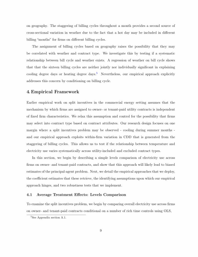
This observational unit provides both cross-sectional and temporal variation in weather. One

source of cross-sectional variation arises from temperature differences across the 32 zip codes in

UI’s service territory. This is made clear in Figure 2 which displays the daily temperature by zip

code between October 2007 and May 2011. Despite the relatively small region, there is visible

cross-sectional variation in daily temperatures with summer temperatures varying between 5 to

10 degrees across zip codes. Variation in our weather variable also occurs because of differences

in billing cycles - which denote the start date and end date of a billing period - across firms. In

our sample, there are 16 unique billing cycles, where firm assignment to a billing cycle is based4CDD measure demand for space cooling services, such as air conditioning, since cooling demand increases as

temperature rises above 65. HDD measure demand for space heating services since heating demand increases astemperature falls under 65.

8

on geography. The staggering of billing cycles throughout a month provides a second source of

cross-sectional variation in weather due to the fact that a hot day may be included in different

billing “months” for firms on different billing cycles.

The assignment of billing cycles based on geography raises the possibility that they may

be correlated with weather and contract type. We investigate this by testing if a systematic

relationship between bill cycle and weather exists. A regression of weather on bill cycle shows

that that the sixteen billing cycles are neither jointly nor individually significant in explaining

cooling degree days or heating degree days.5 Nevertheless, our empirical approach explicitly

addresses this concern by conditioning on billing cycle.

4. Empirical Framework

Earlier empirical work on split incentives in the commercial energy setting assumes that the

mechanism by which firms are assigned to owner- or tenant-paid utility contracts is independent

of fixed firm characteristics. We relax this assumption and control for the possibility that firms

may select into contract type based on contract attributes. Our research design focuses on one

margin where a split incentives problem may be observed - cooling during summer months -

and our empirical approach exploits within-firm variation in CDD that is generated from the

staggering of billing cycles. This allows us to test if the relationship between temperature and

electricity use varies systematically across utility-included and excluded contract types.

In this section, we begin by describing a simple levels comparison of electricity use across

firms on owner- and tenant-paid contracts, and show that this approach will likely lead to biased

estimates of the principal-agent problem. Next, we detail the empirical approaches that we deploy,

the coefficient estimates that these retrieve, the identifying assumptions upon which our empirical

approach hinges, and two robustness tests that we implement.

4.1 Average Treatment Effects: Levels Comparison

To examine the split incentives problem, we begin by comparing overall electricity use across firms

on owner- and tenant-paid contracts conditional on a number of rich time controls using OLS,5See Appendix section A.1.

9

Yit = α+ β1Czt + β2Hzt + θTi + ηit+ γt + εit (1)

The outcome variable is the natural log of electricity use for firm i in billing month t. The regressor

of interest, Ti, is an indicator variable that takes on a value of 1 if firm i is on a utilities-excluded

or tenant-pays contract, and 0 if it is on a utilities-included or owner-pays contract. The variables

Czt and Hzt are average daily cooling and heating degree days for a firm assigned to billing month

t and located in zip code z. We further condition on billing month fixed effects, denoted by γt,

and firm-specific time trends ηi.

Our coefficient of interest, θ, will reflect the average effect of contract type on monthly elec-

tricity use if assignment to a tenant-paid or owner-paid contract is independent of potential

outcomes. In our setting, this identifying assumption seems untenable, since the mechanism by

which firms and buildings are assigned to contract type is likely correlated with fixed firm or

building attributes that also determine electricity use. Tenants may sort into contract type based

on electricity use, the elasticity of their electricity demand, or firm-specific attributes. Another

possibility is that the presence of sub-meters in a building, and hence the ability for owners to

implement tenant-paid contracts, may be co-determined with other fixed building attributes. In

our setting, the decision to construct a building with or without sub-meters may coincide with

other construction decisions such as insulation or window quality that affect electricity use. For

these reasons, buildings and firms on tenant-paid contracts likely differ from those on owner-paid

contracts in ways that affect electricity use. Failure to account for selection into contract type

may result in a biased estimate of θ.

To empirically explore whether selection on fixed firm and building attributes may confound

the estimation of equation (1), we compare firms on owner- and tenant-paid contracts across

a number of observables that we hypothesize may be related to contract type. Tables 1 and 2

report mean characteristics for firms on tenant- and owner-paid contracts, as well as the t-statistic

associated with the difference in means. Motivated by empirical specifications that focus on the

principal-agent problem among all firms and only the largest electricity users, we present these

comparisons for all firms in our sample, Table 1, and firms in the top electricity consumption

decile, Table 2. As shown in Table 1, when we focus on the full sample, the covariates are

10

balanced along the rich set of covariates we observe. However, a comparison of means across the

top decile of electricity users reveals that firms on owner- and tenant-paid contracts differ along a

number of observables, including building height and industry type. These balance statistics cast

doubt on an empirical approach that relies on a levels comparison in electricity use across firms

on different contracts, and lead us to forgo the formal estimation of equation (1).

4.2 Average Treatment Effects: Temperature Gradient

We propose an empirical approach that controls for the possibility that firms and buildings on

owner- and tenant-paid contracts may be systematically different in fixed attributes that also

affect electricity use. We begin with the hypothesis that if a split incentives problem exists, then

it should be observed in differences in cooling across owner- and tenant-paid contracts. We test

this hypothesis by evaluating how electricity use differs in response to a 1 cooling degree day

increase across firms on an owner- versus tenant-paid contract, controlling for firm fixed effects

and weather.

To evaluate the differential effect of a CDD on electricity use across contract type, we estimate

a fixed effects model using OLS,

Yit = β1Czt + β2Hzt + θ1Ti × Czt + θ2Ti ×Hzt + Lt + ηit+ γt + γi + εit (2)

In this specification, the indicator variable for whether tenant i pays its own electric bill is in-

teracted with each of the weather variables, Ti × Czt and Ti ×Hzt. Importantly, this estimating

equation conditions on account fixed effects, γi. This allows us to control for all fixed firm and

building characteristics including those that affect electricity use and may systematically differ

across contract type. We also condition on bill length, Lt, defined as the number of days in a

billing month, to account for differences in weather attributable to variation in bill length across

billing months.

The coefficient, θ1, reflects the differential effect of temperature increases on electricity use

across firms on owner- and tenant-paid contracts. A natural interpretation of θ1 is the change

in demand for air conditioning across contract type in response to warmer temperatures, holding

constant the existing building stock. To estimate this treatment effect, we exploit variation in

11

CDD generated from the staggering of billing cycles, and compare how a firm on an owner-

versus tenant-paid contract responds to this variation netting out fixed firm characteristics. This

approach allows us to account for fixed building and firm attributes systematically correlated with

contract type and electricity use.

Nevertheless, identification of the treatment effect still rests on a key assumption: the response

of electricity use to CDD differs only by unobservables uncorrelated with contract type. When

compared to the levels regression in equation (1), the requirements for identification are less

onerous. This is because equation (2) allows for selection into contract type based on fixed

unobservables. A violation would only occur if attributes systematically correlated with contract

type also exhibit a temperature-dependent impact on electricity use. A second advantage of

our approach is that it explicitly accounts for the possibility that the electricity response to

temperature shocks differs significantly across fixed building attributes (Novan et al. (2017)).

Our empirical approach only breaks down if fixed building attributes that affect electricity use

in a temperature-dependent way are also systematically correlated with contract type. In our

setting, this would occur if, for example, building age was systematically correlated with contract

type, and the electricity response to temperature differed across building vintage.

To examine the plausibility of our main identifying assumption, we augment equation (2) to

account for the possibility that building attributes that differ systematically across contract type

may also impact electricity use along a temperature gradient. Our main estimating equation thus

conditions on interactions between weather and a number of building and firm attributes,

Yit = β1Czt + β2Hzt + θ1Ti × Czt + θ2Ti ×Hzt +ψXi × [Czt, Hzt] + Lt + ηit+ γt + γi + εit (3)

The term ψXi×[Czt, Hzt], denotes a vector of building and firm attributes interacted with heating

and cooling degree days, where Xi includes indicator variables for building type (retail, office,

etc.), firm NAICS code, quartile of building vintage and building stories.6

Our testable hypothesis is that if building attributes confound the temperature response gra-

dient then our coefficient estimate on contract type, θ1, will be sensitive to the inclusion of in-

teractions between temperature and building/firm covariates. If the coefficient estimate remains6We show in Appendix Table A2 that the results are not sensitive to how the characteristic variables are

specified, e.g. in levels, quartile dummies, tertile dummies etc.

12

unchanged after conditioning on these interaction terms, then this provides evidence to support

our main identifying assumption.

4.3 Conditional Average Treatment Effects: Temperature Gradient

A central focus of this paper is whether the size of the split incentives problem varies substan-

tially across firms. One form of heterogeneity in the response to contract type may arise based on

electricity use, since relatively larger users of electricity may devote a larger share of their budget

to electricity expenditures. To empirically examine this form of heterogeneity, we estimate con-

ditional average treatment effects for firms in different deciles of average monthly electricity use.

To implement this, we augment equation (3) and estimate,

Yit = β1d(Czt × 1id) + β2d(Hzt × 1id) + θ1d(Ti × Czt × 1id) + θ2d(Ti ×Hzt × 1id)

+ψdXi × [Czt × 1id, Hzt × 1id] + Lt + ηit+ γt + γi + εit (4)

This estimating equation now includes a vector of indicator variables denoted by 1id that are set

equal to 1 if tenant i has electricity demand in decile d (i.e. d = {1, ..., 10}), and zero otherwise.

These indicator variables are interacted with the weather variables, and the treatment effect of

interest. This allows to us to separately estimate, for each decile of electricity use, the differential

effect of a CDD on demand for electricity across contract type.

4.4 Robustness

To examine the plausibility of our main identifying assumption, we implement two novel robust-

ness tests. The first makes use of a regulatory change allowing buildings to switch contract type

and tests if selection remains an empirical concern. The second applies a new technique proposed

by Oster (2016) to bound our estimated treatment effects.

Our first robustness test takes advantage of a policy change to sub-metering regulations.

Within our sample period, a ban on sub-metering retrofits in Connecticut made selection by

customers and building owners along contract type very costly, if not impossible. For example,

customers desiring attributes of a centrally-metered building may have preferred to pay their

own electricity, and landlords may have preferred to offer tenant-paid energy utilities. However,

13

retrofitting buildings with unit-level electricity meters - a prerequisite for tenant-paid contracting

- was not permitted. In 2013, about two years after our sample period ended, this restriction was

lifted and landlords were allowed to retrofit buildings with sub-meters.

We use building-level tenancy contract information collected a year and a half after the Con-

necticut legislative change to assess whether sorting based on energy consumption preferences

might have occurred once sub-metering retrofits were allowed. Since the legislative change al-

lowed a more flexible re-matching of tenants into contract type, this presents an opportunity to

observe which buildings switched and to directly examine whether controlling for them changes

our baseline results.7 Under the null hypothesis of “no selection,” our estimated treatment ef-

fect should be unchanged after conditioning on the identity of firms switching contract types by

interacting indicator variables for these “switchers” with CDD and HDD.

Our second test uses a new technique proposed by Oster (2016). This method requires the

assumption that the relationship between treatment and unobservables can be recovered from

the relationship between treatment and observables. If this is the case, movements in the coef-

ficient of interest and R-squared levels from the inclusion of control variables inform us about

selection on unobservables. Building on Altonji et al. (2005), Oster (2016) points out that under

the plausible assumption that observable controls share covariance properties with unobservable

variables, omitted variable bias is proportional to coefficient movements, but only if these move-

ments are scaled by changes in R-squared. An ideal scenario in this context is one in which the

treatment coefficient of interest changes very little as new covariates are added, and the regression

R2 approaches its maximal possible value, after accounting for measurement error (Gonzalez and

Miguel (2015)). In this case, the large R2 suggests there is little variation remaining to bias the

coefficient. The Oster approach yields a consistent estimator for the bias-adjusted coefficient of

interest, or an identified set formed by the treatment effect in the fully controlled regression, and

the bias-adjusted effect. We retrieve the Oster bounded set in a post-estimation procedure and7Roughly six percent of customers switched contract types by early 2015, with 34 owners moving to a tenant-paid

contract and 31 transitioning to an owner-paid contract. Switches to owner-paid contracting were not limited priorto the sub-metering policy change, and there are several reasons why owners may switch to owner-paid contracting(see for example Levinson and Niemann (2004)). Importantly, these switches may also be related to the policychange itself - owners who wish to upgrade or reconfigure their building metering infrastructure may need tomaster-meter tenants for a transition period. We control for both types of switches in our empirical specifications.

14

present it in our discussion of the results.

5 Results and Discussion

The reduced form relationship between contract type, firm size, temperature and electricity con-

sumption is presented in Figure 3. It plots electricity consumption against average temperature

within one-degree bins, across both contract types, for the bottom nine deciles of firms in panel

(a), and the top consumption decile in panel (b). Superimposed on each scatter plot is a lowess

fit of consumption on temperature. This figure provides a preview to our formal regression results

and points to three interesting patterns of firm behavior. First, as shown in panel (a), on average

there is almost no discernible difference in consumption by contract type across the distribution

of temperatures in the bottom nine consumption deciles. Second, in the top consumption decile,

shown in panel (b), we observe a significant divergence in usage across contract types, with firms

under owner-paid utility contracts exhibiting higher usage, relative to tenant-paid firms. Third,

this difference in usage becomes more pronounced when air-conditioning demand rises. Consump-

tion levels begin to diverge more sharply once temperature increases beyond approximately 65 F,

the temperature at which demand for cooling typically begins (EPA (2014)).

Table 3 presents our formal regression results. Column (1) shows the effect from the estimation

of equation (2), a regression comparing the differential impact of a weather shock on firms with

a tenant-paid contract type relative to an owner-paid contract, controlling for firm and billing-

month fixed effects and firm-specific time trends. When looking across all firms, we find there

is no difference in the effect of weather shocks on consumption across contract type. In the

remainder of Table 3, we report results that include tenant-paid contract interactions with CDD

and HDD for each consumption decile. Column (2) reports results from the estimation of the

conditional average treatment effects analog of equation (2), and columns (3)-(5), which examine

the robustness of this result to potential confounding factors, report results from the estimation

of equation (4). Column (3) conditions on the interaction of CDD and HDD with building and

industry type; column (4) adds interactions of CDD and HDD with building vintage quartiles;

and column (5) adds controls for the differential effect of temperature shocks among switchers.8

8In Table A2, we also include building storey interactions with cooling and heating degree days; the results are

15

Our results indicate that a split incentives problem leads to overconsumption of energy among

the top decile of electricity consumers. This effect is quantitatively and qualitatively robust to

several specifications, suggesting that firms on a utilities-included contract exhibit a different

dose response function to weather than firms who pay their own utility bills. Focusing on our

preferred specification in column (5), we find that a tenant-paid contract leads to about a 1.4

percent decrease in kWh per average daily CDD for the top decile of electricity consumers. This

translates into about a 3 percent decrease in electricity use among the top decile of users. In

contrast, contract type does not statistically impact consumption decisions for the other 90 percent

of commercial firms. This large divergence in response to contract type based on firm size points

to a first source of heterogeneity in response to treatment, and potentially large savings from the

targeted deployment of a policy instrument.

A second source of heterogeneity results from seasonal variation in the treatment effect. We

find that the split incentive can lead to significant increases in electricity use but only during

the hot summer months. In the summer months, switching from an owner to a tenant-paid

contract would reduce monthly electricity consumption by up to 14 percent. The summer response

is consistent with a framework in which demand for electric air conditioning during these hot

months drives the divergence in the temperature response gradient across owner- and tenant-paid

contracts.9

Though contract type only influences electricity choices for a narrow set of customers during a

concentrated period of time, restructuring contract type has meaningful implications for aggregate

electricity usage. This is because the responsive firms are the largest electricity consumers and

are quite sensitive to hot temperatures. A policy that switched the largest decile of electricity

consuming firms from an owner to tenant-paid contract would result in annual electricity savings

per firm of roughly 19,000 kWh. Comparing these savings to the total quantity of electricity

consumed by all commercial firms in our sample, we find that this policy change would lead to a

1.4 percent reduction in total electricity use.

qualitatively unchanged and the point estimate on our variable of interest increases. Table A2 also shows that ourtreatment effect is not sensitive to the functional form of the building characteristic controls.

9The coefficients on HDD (not reported) are not statistically significant. Since most firms in Connecticut usenatural gas or fuel oil for heating, this is not surprising.

16

We also estimate the effect of contract type on electricity expenditure by estimating our

preferred conditional average treatment effects specification with log monthly bill as the dependent

variable; results are shown in column (6) of Table 3. For the top decile of electricity consumers,

the estimated treatment effect is a 1.2 percent decrease in the monthly bill per CDD. The value

of total bill savings among these high consumers is approximately $310 per summer month. On

average, this represents a 10 percent reduction in electricity expenditure.

To further gauge the robustness of our results to potential selection on unobservables, we

apply the bounds analysis proposed by Oster (2016). We make an equal selection assumption,

which implies that any residual omitted variable bias is a function of: (i) the treatment coefficient

before and after the inclusion of covariates; (ii) R-squared values before and after the inclusion

of covariates; and (iii) the maximum theoretically possible R-squared, namely from a regression

on consumption and all possible observable and unobservable controls. This maximum R-squared

may be less than 1 if there is measurement error.

Given our rich set of controls, the equal selection assumption is likely conservative, as it as-

sumes that any remaining unobservables are at least as important as the observables in explaining

the treatment (Oster (2016), Altonji et al. (2005)). Table 4 reports the identified set estimates

from two different specifications with log usage and log bill as the dependent variables, respec-

tively, corresponding to the fully controlled specifications reported in columns (5) and (6) of Table

3.10 As shown in this table, we continue to detect a split incentives effect after accounting for

any remaining selection on unobservables. A tenant-paid contract induces at minimum monthly

electricity and bill savings of 0.7 and 0.6 percent per CDD, respectively.11

5.1 Generalizability

There are roughly 18 million commercial electricity customers in the U.S. and 5.6 million com-

mercial buildings ((EIA (2017), EIA (2012)). In this section, we explore the similarity of the

subpopulation under study here to the full population of commercial sector tenanted buildings in

the U.S. Understanding if our estimates apply to the broader population of large commercial users10These set estimates assume that the maximum possible R2 is 0.98, given the estimated 2 percent measurement

error in electricity meter readings (Dong et al. (2005), Reddy et al. (1997)).11All the energy and bill savings ranges reported in the following sections are based on these Oster identified set

estimates.

17

provides insights into the potential energy savings from restructuring electricity contracts from

owner- to tenant-pay. To demonstrate the broader relevance of our results, we proceed in three

steps. First, we make use of a representative data set of national commercial building attributes

to show that, along important observables, the data source used in our analysis is representative

of building attributes throughout the U.S. Second, we focus exclusively on the database used in

our analysis, and illustrate that the distribution of attributes for commercial buildings in Con-

necticut is similar to those in the broader U.S. Third, we then compare contract types and energy

intensity in commercial buildings in Connecticut to those across the U.S. We use these contract

type statistics in Section 5.2 to estimate the energy savings implied by our treatment effect.

In the first step, we demonstrate that the building database used in our analysis is a represen-

tative sample of building attributes in the U.S. Our empirical sample uses data on contract type

and building attributes collected from the CoStar group. An advantage of the data collected by

the CoStar group is that it includes buildings throughout the U.S., totaling about 97 percent of

tenanted buildings. We compare three important building characteristics in the CoStar dataset

- building height, age and size - to the Energy Information Administration’s Commercial Build-

ing Energy Consumption Survey (CBECS), a nationally representative data set on attributes in

both owner and tenant occupied commercial buildings. The CBECS and CoStar datasets are

very similar in building height and vintage. While the average CoStar building is larger than

the CBECS average, this may be representative of the larger size of leased buildings compared

to owner-occupied buildings (EIA (2012)). These similarities in observables, along with the fact

that the CoStar database is reflective of leased commercial buildings in the U.S., lends confidence

to the national representativeness of the CoStar data.

Second, we show that within the CoStar data there is strong overlapping support in the

distributions of measurable building characteristics between Connecticut and the rest of the United

States. The overlapping support of building characteristics can be seen in Figure 4. Ideally, we

would compare attributes of buildings in the top 10th percentile of electricity usage in Connecticut

to those in the U.S. This is not feasible since CoStar does not collect electricity use as a variable.

Instead we display the full distribution for both Connecticut and the U.S. of building attributes

that we hypothesize are highly correlated with electricity use: square feet, number of stories,

18

and year of construction. For all three variables, significant overlap exists, despite some apparent

differences (e.g. Connecticut has a lower proportion of very small buildings). As we discuss below,

differences between the Connecticut sample and the broader population imply that the commercial

split incentives problem is potentially even larger in the rest of the U.S. than in Connecticut.

Finally, comparing the composition of contract types and energy intensity in Connecticut to

the rest of the U.S. once again leads to the conclusion that the split incentive problem is likely

at least as large outside of Connecticut as it is within Connecticut. Approximately 34 percent

of commercial, non-government floorspace in New England is leased, as compared to 39 percent

nationwide (EIA (2012)).12 The CoStar database reports contract type for commercial lessees

nationwide, differentiating between contracts that transmit price incentives to tenants and those

that do not. In our Connecticut sample, about 15 percent of commercial lessees are on owner-

pay contracts, as compared to 25 percent nationwide.13 With respect to energy intensity, New

England is the least energy-intense region in the nation when measured by kWh per square foot

of commercial building space (EIA (2012)). When we condition on buildings in which owners pay

for electricity, New England is still well below the national average: 11.6 kWh per square foot in

New England versus 14.4 nationwide.

Proportionally, less commercial floorspace is rented in New England than nationwide; a higher

proportion of commercial renters are on owner-pay contracts in the rest of the U.S.; and the energy

intensity per commercial square foot is higher in regions outside of New England. Thus in terms

of the magnitude of the potential split incentives problem in the commercial segment, it is likely

to be larger per square foot of commercial building space in the rest of the country than it is in

Connecticut.12EIA’s Commercial Building Energy Consumption Survey (EIA (2012)) publicly reports this variable at the

regional level, rather than by state.13The nationwide figure is even larger if we include contracts with a prorated utility payment for all building

occupants, whereby tenants pay a weighted average of the building’s utility bill based on the square feet occupied.In this contractual arrangement, tenants do not pay for the marginal cost of their energy use and large consumersbenefit by paying less than their share of utilities. Conservatively, we categorize these as ‘owner-paid’ in ourpaper, though only about 3 percent of tenants are on a prorated contract in our sample. Nationwide, about 20percent of tenant contracts include a prorated utility payment. In Section 5.2 we treat these figures under the mostconservative assumptions.

19

5.2 Quantifying Benefits from Aligning Split Incentives

Under conservative assumptions, restructuring rental contracts for the largest ten percent of

commercial firms nationwide would produce energy savings roughly three times those achieved

from restructuring rental contracts for all residential users who don’t pay for their utilities. This

conclusion is derived from the following calculation. There are 130 million residential electricity

customers in the U.S., of whom 10.4 million rent dwellings with utilities included (EIA (2009)).

Assuming they conserve 0.7 percent of their electricity when exposed to a non-zero price (Levinson

and Niemann (2004)), total residential savings are 142 million kWh per year. By comparison, there

are approximately 18 million commercial sector electric customers in the U.S. (EIA (2017)), 39

percent of which rent their building space (based on the share of tenanted buildings in the U.S.

in EIA (2012)). Suppose 25 percent of those (1.74 million) have an owner-paid utilities contract.

The top consumption decile, 174,000 customers, save a total of 411 gigawatt-hours per year (1.4

percent based on our preferred empirical estimates) from a switch to tenant-pay contracts. This

amounts to 289 percent percent of the residential sector analog. Under much more conservative

assumptions, this number falls to 177 gigawatt-hours per year, or 125 percent of the residential

sector analog.14

Addressing the commercial split incentives problem has relatively high benefit-to-cost. Using

data on the costs of sub-metering, we estimate the payback period from sub-metering individual

units and shifting to a tenant-paid contract. Sub-meter costs range from $250-$1000 per unit

(Pike Research (2012), White (2012), Millstein (2008)). Given the average estimated annual bill

savings of $970 (the average of the bill savings obtained using the Oster identified set estimates)

and assuming a unit-level sub-meter cost of $625 (the average of the sub-meter cost ranges cited

above), the payback period is less than one year, even after allowing for installation costs. This

is well below the payback threshold for most firms’ energy conservation investments (Anderson14We reduce the fraction of renters from 39 percent to 36 percent to reflect the share of tenanted floor space,

rather than the share of tenanted buildings (EIA (2012)), use the average electricity use across all large firms (notjust those on owner-pay contracts, who use more electricity), and adjust our treatment effect estimate down by onestandard deviation. These changes are multiplicative and thus result in an extremely conservative estimate. Asmentioned in the previous section, it is likely that the base case comparison to the residential sector understates therelevance of our results to the U.S. commercial sector as a whole, so the conservative estimate should be interpretedas a lower bound.

20

and Newell (2004)).15 With a unit- or firm-level sub-meter cost of $625, a cost which would

be incurred up-front, and an average annual treatment effect of 19,000 kWh saved among high

consuming firms, the cost effectiveness is 3.3 cents per kWh after the first year, 1.6 cents per kWh

after two years, and 1.1 cents after 3 years, assuming the annual electricity savings persist at the

same level.

To calculate the reduction in external damages from a switch to tenant-paid contracts, we

convert energy savings into avoided CO2 and PM2.5 emissions, and then monetize the reduction

in emissions.16 To quantify CO2 we use the Environmental Protection Agency’s eGRID database

which provides 2009 emission rates for the New England subregion, measured as tons emitted per

MWh of electricity produced.17 The energy savings translate into CO2 savings of between 615 to

1200 thousand tons per year. To give a sense of scale, this is between 3.3 to 6.6 times the average

annual savings achieved from yearly Weatherization Assistance Program (WAP) retrofits.18 The

PM2.5 emission rates estimate is obtained from Connors et al. (2005). Marginal damage esti-

mates for PM2.5 come from Muller and Mendelsohn (2007), and marginal CO2 damages are from

IWGSCC (2015).

The upper and lower bound estimates for avoided pollution-related external costs are presented

in Table 5. As shown in columns (1) and (2), the per firm value of avoided damages ranges from

$102 to $204. In columns (3) and (4) we add to this the estimated bill savings of $677 to $1265 per

firm-year. Using this measure, the annual firm-level social benefit of switching from an owner- to

tenant-paid contract is between $779 and $1469. Finally, in columns (5) and (6) we measure the

value of the energy savings using the avoided marginal cost of electricity (in place of bill savings).

We use this approach to net out fixed costs. Fixed costs are not avoided costs in this setting,15In most states sub-meter system costs can be recovered through surcharges on tenant utility bills. This enables

owners to recover their investments costs. If the owner’s surcharge doesn’t recover the full value of the savings, thepayback period may be longer, but our estimates would still represent a social payback period.

16We do not include damages from NOx and SO2 emissions, given regional and federal regulations in place duringour sample time frame. Assuming the emissions caps for these regulations were binding, a reduction in electricityconsumption would not reduce aggregate emissions but reallocate them to a different source. While CO2 emissionswere also regulated through the Regional Greenhouse Gas Initiative from 2009 onwards, the early phase of thisprogram did not have a binding cap (CRS (2017)).

17The eGRID database is available at the EPA’s website at www.epa.gov/energy/egrid.18An average of 175,000 WAP retrofits are performed every year, which save approximately 1.06 tons of CO2

per household per year (Fowlie et al. (2015), DOE (2017), EIA (2010)). These retrofits therefore save 186,000 tonsof CO2 every year.

21

since they will be recovered by the utility from other customers under the cost-plus regulatory

structure in Connecticut. Our measure of avoided marginal cost is the average hourly locational

marginal price for Connecticut over the sample period, $59.42.19 Total social benefits using

avoided marginal costs are between $676 and $1346. Given that the average cost of a sub-meter

is $625, sub-metering retrofits are likely net beneficial from a social perspective.

5.3 The Non-Response of Most Commercial Firms

While we estimate that contract type has a sizable effect on electricity use for the largest firms,

one unanswered question is why the remaining 90 percent of commercial firms do not respond

to contract type. In our view, the most likely explanation is that even when tenants face the

costs of their energy consumption choices, the net benefits of decreasing electricity consumption

or investing in energy efficiency are negative. This is consistent with a growing strand of research

that documents negative realized net benefits from energy efficiency investments (Hassett and

Metcalf (1999), Fowlie et al. (2015)). In this section, we provide evidence for this hypothesis

by performing a coarse cost-benefit analysis for a common energy-saving behavioral change. We

then go on to document other potential explanations for why firms may not mitigate their energy

consumption under a tenant-paid contract.

Let us consider the electricity choices of an office building, the sector that makes up the largest

share of buildings in our sample. Overcooling and overheating are common in office buildings, and

some occupants’ behavioral responses, such as running personal heaters or fans, also contribute

to increasing energy consumption. Derrible and Reeder (2015) suggest that overcooling increases

electricity consumption by 8 percent per year, and Sanchez et al. (2007) estimate portable heaters

consume 329 kWh per year. Using these numbers, for the bottom nine deciles of our sample,

the combination of overcooling and space heating amounts to 4,300 kWh of annual electricity

consumption, or $530 on an annual basis. Since addressing overcooling would likely require hiring

a property manager or engineer to monitor and adjust air conditioner and chiller operation, the

total cost of avoiding overcooling may well exceed the $530 reduction in expenditure.

Other explanations could also account for the lack of a treatment effect across most firms.19Our data source is the New England Independent System Operator (NE-ISO), www.iso-ne.com.

22

One possibility is (potentially rational) inattention leading to unresponsiveness among commercial

firms (Jessoe and Rapson (2015)). Comparing the $677 to $1265 annual bill saving from a tenant-

paid contract to the average commercial unit size in Connecticut, 14,000 square feet, suggests

an average annual bill saving of about 4.8 to 9 cents per square foot. This represents about

0.2 percent of the average annual revenues per square foot in office and retail industries and

highlights that the savings smaller firms forgo likely represent a small share of their annual sales.

After accounting for the time and effort required to accurately assess the energy savings from

different energy efficiency investments, firms may be rationally inattentive to potential energy

savings since the savings are comparatively quite small (Sallee (2014)).

6. Conclusion

We measure the “split incentive” effect of tenancy contract type using a unique empirical setting

and dataset of tenancy contracts and energy use among commercial sector clients. Our empirical

framework compares how temperature shocks impact electricity consumption across firms on

owner- and tenant-paid contracts. Importantly, it helps us to overcome the well-known empirical

challenge of separately identifying the split incentives problem from selection on fixed attributes.

Our approach consists of three steps to probe and address the main identification challenge:

selection on unobservables that affect electricity use along a temperature gradient. We allow for a

heterogeneous temperature response gradient along several dimensions by including interactions

between temperature and building attributes that may be correlated with energy consumption,

testing for selection by taking advantage of a state-level change in metering regulations, and

accounting for any potential remaining correlations between unobservable characteristics and the

treatment using the Oster (2016) identified set approach.

Our results indicate heterogeneous returns to a tenant-paid contract, with a positive and

significant effect of contract type only in the top decile of electricity consuming firms. The results

are consistent with privately optimal decision-making since the bill savings from conservation

behavior are relatively small across most of the consumption distribution. Hence, they are likely

not large enough to justify energy efficiency investments or behavioral changes.

The result implies a strong policy case for encouraging tenant-paid energy contracting among

23

large commercial and industrial customers. For the largest decile of electricity consumers, we

find that firms who pay their own utility bills consume about 3 percent less electricity annually

than tenants whose utility bills are bundled into rents, and save between $677 and $1265 on their

annual electricity bills. These reductions lead to a 1.4 percent saving in total electricity consumed

by all firms in our sample, and a 3 percent saving for firms in the top consumption decile. These

savings generate annual external benefits between $102 and $204. The payback period from sub-

metering and switching to a tenant-paid contract is less than one year, and a targeted policy of

sub-metering and tenant-paid contract promotion would likely be a net beneficial addition to the

portfolio of energy conservation and greenhouse gas mitigation strategies utilized by policymakers.

Several features of our findings lead us to have conviction about the potential importance

of commercial split incentives in electricity. The commercial split incentives problem is large

and likely even more important in the rest of the U.S. than in Connecticut, due to the higher

prevalence of leased space and owner-pay contracts. If our sample is representative, then the

public and private benefits both independently provide an efficiency case for facilitating sub-

metering and tenant-pay contracts among top consumers. Moreover, if sub-metering occurs after

the building is constructed, features of the building envelope are predetermined and thus less likely

to be exposed to underinvestment in energy efficiency that may arise from tenant-pay contracts.

Finally, the sheer size of large commercial electricity customers distributes the fixed cost per kWh

conserved due to sub-metering much more efficiently than can occur in the residential case. While

it would of course be beneficial to run a large-scale randomized trial to reduce the possibility of

erroneous conclusions, we view a strong case for policy action or, at the very least, a concerted

effort to resolve uncertainties about the policy case.

24

References

Allcott, Hunt (2011) “Social Norms and Energy Conservation,” Journal of Public Economics, Vol. 95, pp.1082–1095.

Allen, P.V., P.C. Lacourciere, and R.M. Shapiro (2007) “Submetering of Electricity for Commercial Build-ings,” November, Thellen LLP, published by Mondaq Ltd.

Altonji, Joseph G., Todd Elder, and Christopher R. Taber (2005) “Selection on Observed and UnobservedVariables: Assessing the Effectiveness of Catholic Schools,” Journal of Political Economy, Vol. 113, pp.151–184.

Anderson, Soren T. and Richard G. Newell (2004) “Information programs for technology adoption: thecase of energy-efficiency audits,” Resource and Energy Economics, Vol. 26, pp. 27–50.

ASHRAE (2012) “Proposed Addendum to Standard 90.1 2010, Energy Standard for Low-Rise Buildings Ex-cept Low-Rise Residential Buildings,” American Society of Heating, Refrigeration and Air-ConditioningEngineers.

Basarir, Murat Nihat (2010) “Energy Appraisal of Retail Units: Assessing the Effect of Door Operation onEnergy Consumption and Thermal Comfort,” M.Phil thesis in Engineering, University of Cambridge.

Blumstein, Carl, Betsy Krieg, Lee Schipper, and Carl York (1980) “Overcoming Social and InstitutionalBarriers to Energy Conservation,” Energy, Vol. 5, pp. 355–371.

Connors, S., K. Martin, M. Adams, E. Kern, and B. Asiamah-Adjei (2005) “Emissions Reductions fromSolar Photovoltaic (PV) Systems,” MIT Laboratory for Energy and the Environment report 2004-003.

Cross, Phillip S. (1996) “N.Y. Allows Gas Submetering for C&I Customers,” Fortnightly Magazine, Novem-ber 15, 1996.

CRS (2017) “The Regional Greenhouse Gas Initiative: Lessons Learned and Issues for Congress,” Con-gressional Research Service.

Davis, Lucas W. (2012) “Evaluating the Slow Adoption of Energy Efficiency Investments: Are RentersLess Likely to Have Energy Efficient Appliances?” in Don Fullerton and Catherine Wolfram eds. TheDesign and Implementation of U.S. Climate Policy.

Derrible, Sybil and Matthew Reeder (2015) “The Cost of Over-Cooling Commercial Buildings in the UnitedStates,” Energy and Buildings, Vol. 108, pp. 304–306.

DOE (2017) “The Weatherization Assistance Program: An American Industry,” Office of Energy Efficiencyand Renewable Energy, Department of Energy.

Dong, Bing, Siew Eang Lee, and Majid Haji Sapar (2005) “A Holistic Utility Bill Analysis Method forBaselining Whole Commercial Building Energy Consumption in Singapore,” Energy and Buildings, Vol.37, pp. 167–174.

EIA (2009) “Residential Energy Consumption Survey,” Energy Information Administration.

EIA (2010) “Weatherization Assistance Program: Know the Facts,” February 2010 Short Term EnergyOutlook, Energy Information Administration.

EIA (2012) “Commercial Building Energy Consumption Survey,” Energy Information Administration.

EIA (2017) “Electric Power Monthly,” Energy Information Administration.

25

Elinder, Mikael, Sebastian Escobar, and Ingel Petre (2017) “Consequences of a price incentive on freeriding and electric energy consumption,” Proceedings of the National Academy of Sciences, Vol. 114.

EPA (2014) “Heating and Cooling Degree Days,” Environmental Protection Agency,http://bit.ly/1RywQQI.

Fowlie, Meredith, Michael Greenstone, and Catherine Wolfram (2015) “Do Energy Efficiency InvestmentsDeliver? Evidence from the Weatherization Assistance Program,” Working Paper.

Gillingham, Kenneth, Matthew Harding, and David Rapson (2012) “Split Incentives in Household EnergyConsumption,” The Energy Journal, Vol. 33(2), pp. 37–62.

Gillingham, Kenneth and Karen Palmer (2014) “Bridging the Energy Efficiency Gap: Insights for Policyfrom Economic Theory and Empirical Analysis,” Review of Environmental Economics and Policy, Vol.8.

Gonzalez, Felipe and Edward Miguel (2015) “War and Local Collective Action in Sierra Leone: A Commenton the Use of Coefficient Stability Approaches,” Journal of Public Economics, Vol. 128, pp. 30–33.

Hartford Business Journal (2013) “CT approves submetering, fines N.H. landlord. June 10, 2013,” retrievedDecember 2017.

Hassett, Kevin A. and Gilbert E. Metcalf (1999) “Measuring the Energy Savings from Home ImprovementInvestments: Evidence from Monthly Billing Data,” The Review of Economics and Statistics, Vol. 81,pp. 516–528.

IBE (2011) “High-Performance Tenant Build-out: A Primer for Tenants,” Institute for Building Efficiency,Johnson Controls.

Ito, Koichiro (2014) “Do Consumers Respond to Marginal or Average Price? Evidence from NonlinearElectricity Pricing,” American Economic Review, Vol. 104, pp. 537–563.

IWGSCC (2015) “Technical Support Document: Technical Update on the Social Cost of Carbon forRegulatory Analysis - Under Executive Order 12866,” Interagency Working Group on Social Cost ofCarbon, United States Government.

Jaffe, Adam and Robert Stavins (1994) “Energy Efficiency Investments and Public Policy,” The EnergyJournal, Vol. 15, pp. 43–65.

Jessoe, Katrina and David Rapson (2015) “Commercial and Industrial Demand Response Under MandatoryTime-of-Use Electricity Pricing,” Journal of Industrial Economics, Vol. 63, pp. 397–421.

Jessoe, Katrina, David Rapson, and Jeremy B. Smith (2014) “Towards Understanding the Role of Price inResidential Electricity Choices: Evidence from a Natural Experiment,” Journal of Economic Behaviorand Organization, Vol. 107.

Kahn, Matthew E., Nils Kok, and John M. Quigley (2014) “Carbon emissions from the commercial buildingsector: The role of climate, quality, and incentives,” Journal of Public Economics, Vol. 114, pp. 1–12.

Levinson, A. and S. Niemann (2004) “Energy use by apartment tenants when landlords pay for utilities,”Resource and Energy Economics, Vol. 26, pp. 51–75.

Millstein, Don (2008) “Submetering can measure energy use more accurately in shopping centers,” RetailConstruction Magazine, January/February 2008.

26

Muller, Nicholas Z. and Robert Mendelsohn (2007) “Measuring the damages of air pollution in the UnitedStates,” Journal of Environmental Economics and Management, Vol. 54, pp. 1–14.

Murtishaw, S and J Sathaye (2006) “Quantifying the Effect of the Principal-Agent Problem on U.S.Residential Energy Use,” Lawrence Berkeley National Laboratory report LBNL-59773.

Myers, Erica (2014) “Asymmetric Information in Residential Rental Markets: Implications for the EnergyEfficiency Gap,” Energy Institute at Haas Working Paper 246.

NJAA (2005) “Water Conservation and Economy in New Jersey through Sub-Metering of Water in Multi-Family Rental Housing,” New Jersey Apartment Association.

Novan, Kevin, Aaron Smith, and Tianxia Zhou (2017) “Residential Building Codes Do Save Energy:Evidence From Hourly Smart-Meter Data,” June, Working Paper.

Oster, Emily (2016) “Unobservable Selection and Coefficient Stability: Theory and Evidence,” Forthcom-ing, Journal of Business Economics and Statistics.

Pike Research (2012) “Electricity Submeters,” Research Report.

Reddy, T.A., N.F. Saman, D.E. Claridge, J.S. Haberl, W.D. Turner, and A. Chalifoux (1997) “BaseliningMethodology for Facility-Level Monthly Energy Use - Part 1: Theoretical Aspects,” ASHRAE Trans.,Vol. 103.

Sallee, James (2014) “Rational Inattention and Energy Efficiency,” Journal of Law and Economics, Vol.57, pp. 781–820.

Sanchez, Marla, Carrie Webber, Richard Brown, John Busch, Margaret Pinckard, and Judy Robertson(2007) “Space Heaters, Computers, Cell Phone Chargers: How Plugged In Are Commercial Buildings?,”Lawrence Berkeley National Laboratory Report No. 62397.

Treitler, Marc (2000) “Submetering: What You Don’t Know Can Cost You,” July, Units Magazine, Na-tional Apartment Organization.

USGBC (2013) “LEED v4 User Guide,” U.S. Green Building Council.

White, Evan (2012) “Utilities in Federally Subsidized Housing,” Goldman School of Public Policy and UCBerkeley Law at Boalt Hall.

27

Figure 1: UI Territory

Notes: United Illuminating’s service territory. It offers electricity distribution services to 17 counties in Connecticut,an area totaling 335 square miles.

28

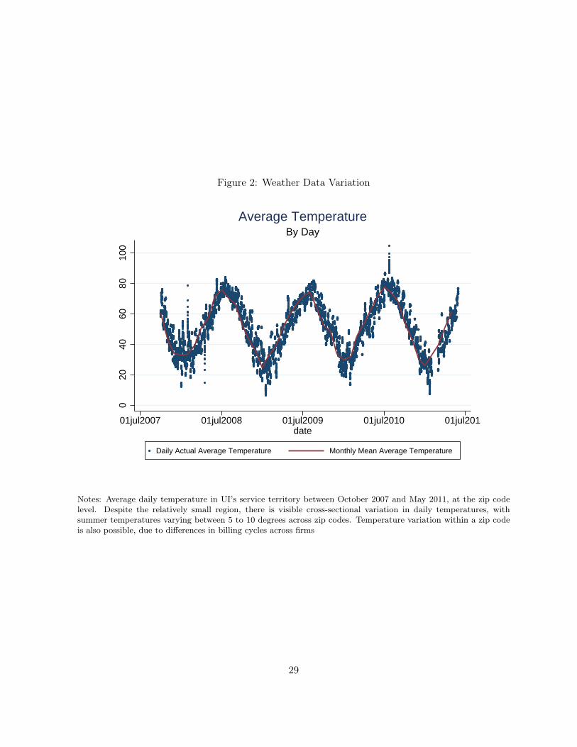
Figure 2: Weather Data Variation

020

4060

8010

0

01jul2007 01jul2008 01jul2009 01jul2010 01jul2011date

Daily Actual Average Temperature Monthly Mean Average Temperature

By DayAverage Temperature

Notes: Average daily temperature in UI’s service territory between October 2007 and May 2011, at the zip codelevel. Despite the relatively small region, there is visible cross-sectional variation in daily temperatures, withsummer temperatures varying between 5 to 10 degrees across zip codes. Temperature variation within a zip codeis also possible, due to differences in billing cycles across firms

29

Figure 3: Consumption By Contract Type

(a) Bottom Nine Deciles

.2.6

11.

41.

8

Aver

age

Dai

ly C

onsu

mpt

ion

(000

s kW

h)

40 50 60 70 80 90

Average Monthly Temperature

Tenant-Paid Scatter Owner-Paid ScatterTenant-Paid Lowess Owner-Paid Lowess

(b) Highest Consumption Decile

.2.6

11.

41.

8

Aver

age

Dai

ly C

onsu

mpt

ion

(000

s kW

h)

40 50 60 70 80 90

Average Monthly Temperature

Tenant-Paid Scatter Owner-Paid ScatterTenant-Paid Lowess Owner-Paid Lowess

Notes: Each scatter plot presents monthly electricity consumption against average temperature within 1-degreebins, for the bottom nine decile of firms in panel (a), and the top consumption decile in panel (b). The observationsare color-coded by contract type, in both the bottom nine deciles (panel (a)), and the top consumption decile (panel(b)). The solid lines are a lowess fit of the same data.

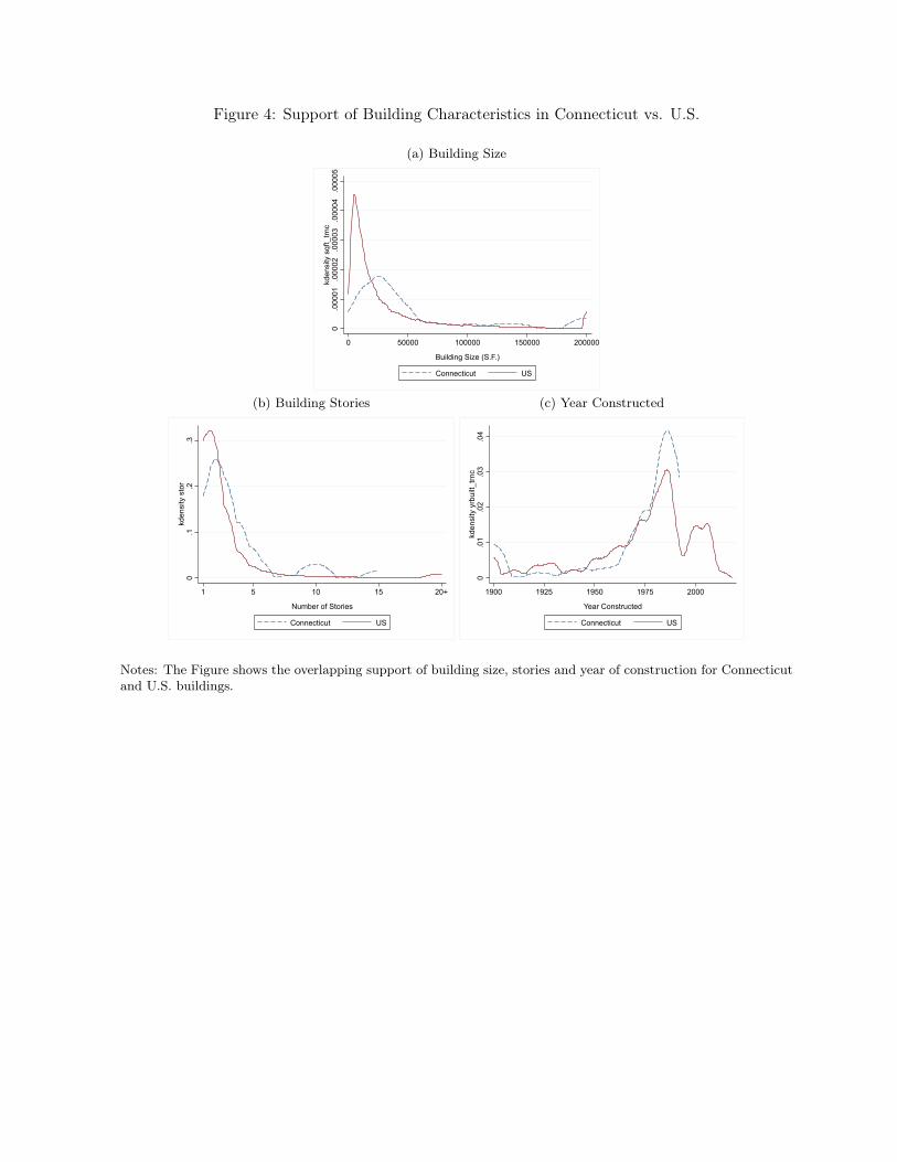
Figure 4: Support of Building Characteristics in Connecticut vs. U.S.

(a) Building Size

0.0

0001

.000

02.0

0003

.000

04.0

0005

kden

sity

sqf

t_trn

c

0 50000 100000 150000 200000

Building Size (S.F.)

Connecticut US

(b) Building Stories

0.1

.2.3

kden

sity

sto

r

1 5 10 15 20+

Number of Stories

Connecticut US

(c) Year Constructed

0.0

1.0

2.0

3.0

4kd

ensi

ty y

rbui

lt_trn

c

1900 1925 1950 1975 2000

Year Constructed

Connecticut US

Notes: The Figure shows the overlapping support of building size, stories and year of construction for Connecticutand U.S. buildings.

Table 1: Summary statistics and covariate balance in full sample

1

t-Statistic

Mean St. Dev. Mean St. Dev.

kW 27.3 42.9 33.5 61.4 0.42 0.41726998

kWh (000s) 7.7 13.8 9.0 17.1 0.31 0.31104742

Bill ($) 627 999 720 1220 0.31 0.31120586

Bill Length 30.3 1.3 30.4 1.3 0.30 0.30456453

Building S.F. (000s) 57.2 59.7 66.8 93.6 0.43 0.42920962

Year Built 1974 26 1968 33 0.76 0.75580493

Building Stories 2.6 1.6 3.4 3.1 1.09 1.09484174

Industry 0.12 0.33 0.10 0.31 0.25 0.25288921

Trade, Accommodation 0.15 0.36 0.12 0.33 0.35 0.35464475

Finance, Real Estate, Management 0.47 0.36 0.55 0.50 0.66 0.66249162

Education, Health, Pub. Admin. 0.19 0.36 0.18 0.38 0.11 0.10526796

Entertainment, Recreation, Services 0.07 0.36 0.05 0.21 0.33 0.32680661

North 0.40 0.49 0.36 0.48 0.33 0.32918993

South 0.60 0.49 0.64 0.48 0.33 0.32918993

City 0.30 0.46 0.31 0.46 0.09 0.08618731

ObservationsFirms

All Firms

6,658 178

Owner-Paid

34,304 948

Tenant-Paid

Notes: The table shows the mean and standard deviations for the observed covariates, for tenant-paid and owner-paid contracts, respectively. The last column shows the value of the t-statistic for the null hypothesis of equalmeans between the two contract types.

32

Table 2: Summary statistics and covariate balance in top consumption decile

1

t-Statistic

Mean St. Dev. Mean St. Dev.

kW 132.4 71.2 164.2 120.9 1.11 1.10712455

kWh (000s) 40.6 24.1 44.5 34.1 0.47 0.47440112

Bill ($) 3002 1759 3276 2403 0.47 0.4713521

Bill Length 30.4 1.3 30.4 1.3 0.03 0.03104636

Building S.F. (000s) 86.8 79.7 144.9 146.4 1.68 1.67870445

Year Built 1978 19 1973 24 0.85 0.85394858

Building Stories 3.0 2.4 6.1 5.1 2.61* 2.60561878

Industry 0.22 0.41 0.18 0.39 0.40 0.40298272

Trade, Accommodation 0.09 0.28 0.04 0.20 0.92 0.91796421

Finance, Real Estate, Management 0.46 0.50 0.77 0.42 2.83* 2.82619725

Education, Health, Pub. Admin. 0.09 0.29 0.00 0.00 2.96* 2.96050097

Entertainment, Recreation, Services 0.15 0.35 0.00 0.00 4.09* 4.08831086

North 0.39 0.49 0.27 0.44 1.06 1.05950465

South 0.61 0.49 0.73 0.44 1.06 1.05950465

City 0.27 0.45 0.40 0.49 1.07 1.06635796

ObservationsFirms 91 19

Top Decile Firms

Owner-PaidTenant-Paid

3,202 703

Notes: The table shows the mean and standard deviations for the observed covariates, for tenant-paid and owner-paid contracts, respectively. The last column shows the value of the t-statistic for the null hypothesis of equalmeans between the two contract types. Asterisks indicate a rejection of the null at the 5 percent level of significance.

33

Table 3: Split Incentive Effect By Consumption Decile

1

Dependent variable: Log Bill(1) (2) (3) (4) (5) (6)

Tenant x CDD -0.00001(0.00009)

Tenant x CDD (10th Dec.) -0.013** -0.015*** -0.015** -0.014** -0.012**(0.006) (0.006) (0.006) (0.006) (0.005)

Tenant x CDD (9th Dec.) 0.001 0.004 0.005 0.005 0.004(0.009) (0.010) (0.009) (0.009) (0.009)

Tenant x CDD (8th Dec.) -0.001 0.005 0.005 0.004 0.002(0.007) (0.007) (0.007) (0.007) (0.005)

Tenant x CDD (7th Dec.) -0.004 -0.001 0.003 0.003 0.001(0.007) (0.008) (0.007) (0.007) (0.005)

Tenant x CDD (6th Dec.) 0.010 0.014* 0.011 0.012 0.009*(0.008) (0.007) (0.007) (0.007) (0.005)

Tenant x CDD (5th Dec.) 0.003 0.005 0.005 0.005 0.004(0.007) (0.008) (0.007) (0.007) (0.005)

Tenant x CDD (4th Dec.) 0.009 0.011 0.012 0.012 0.009(0.011) (0.011) (0.010) (0.010) (0.006)

Tenant x CDD (3rd Dec.) -0.017 -0.017 -0.012 -0.012 -0.006(0.014) (0.014) (0.013) (0.013) (0.008)

Tenant x CDD (2nd Dec.) 0.005 0.004 0.006 0.006 0.006(0.010) (0.010) (0.009) (0.010) (0.005)

Tenant x CDD (1st Dec.) -0.010 -0.009 -0.009 -0.009 -0.002(0.012) (0.012) (0.011) (0.012) (0.007)

Account & Time F.E.s, Acct. Trend YES YES YES YES YES YESCharacteristics Interactions NO NO YES YES YES YESCharacteristics Interactions w/ Year-Built NO NO NO YES YES YESSwitchers Controls NO NO NO NO YES YES

Observations 40,962 40,962 40,962 40,962 40,962 40,962Accounts 1,126 1,126 1,126 1,126 1,126 1,126R-squared (within) 0.067 0.076 0.088 0.093 0.093 0.26

Log Usage

Notes: The dependent variable in columns (1-5) is the natural log of electricity use in a billing month, and in column(6) it is the natural log of the electricity bill in a billing month. Results are reported from an OLS regression.Column (1) presents results without decile interactions, and columns (2)-(6) include results across consumptiondeciles. Additional controls included in all regressions are cooling degree days, heating degree days, and heatingdegree days interacted with contract type. Column (3) further conditions on cooling and heating degree daysinteracted with building type and NAICS code dummies. Column (4) adds interactions of quartile of year-builtwith cooling and heating degree days. Column (5) also includes switchers dummies interacted with cooling andheating degree days. Standard errors clustered at the building level are in parentheses, ***p<0.01, ** p<0.05, *p<0.1.

Table 4: Oster Bounds for Monthly Usage and Bill

1

Lower BoundUpper Bound

Lower BoundUpper Bound

Identified Set Estimate

Log Usage

-0.014-0.007

Log Bill

Identified Set Estimate

-0.012-0.006

Notes: The Oster bounds present an identified set of treatment effect coefficients (interpreted as savings per averagedaily CDD) by accounting for residual omitted variable bias through an equal selection assumption. The omittedvariable bias is assumed to be a function of the treatment coefficient and R-squared values before after the inclusionof covariates, as well as the maximum theoretically possible R-squared, namely from a regression on consumptionand all possible observable and unobservable controls.

35

Table 5: External Benefits and the Value of Energy Savings Per Firm

Low $ 0High $ Low $ High $ Low $ High $

(1) (2) (3) (4) (5) (6)

PM2.5 0.38 00.76 677 1266 574 1143

CO2 101.95 000202.91 779 1468 676 1345

Total 102.33 000203.67 779 1469 676 1346

Social'Benefits'Calculations:New'England'(eGRID'NEWE'region)'emissions'factors,'tons'per'kWh Values

NOx 0.00000026SO2 0.00000071CO2 0.00036420

PM2.5 0.00000003

Total'emissions'saved'per'tenantSpaid'firm'during'summer'months,'in'tons,'using'Oster'bounds High LowNOx 0.00500 0.00251SO2 0.01361 0.00684CO2 6.99706 3.51544

PM2.5 0.00064 0.00032

Total'damages,'using'Oster'bounds High LowNOx 1.49937 0.75331SO2 16.33161 8.20526CO2 202.91482 101.94763

PM2.5 0.76283 0.38326WAP'calculations 221.50863 111.28946CO2'savings:emissions'factors'times'per'firm'electricity'savings'times'number'of'firms

High Low1224486 615201

WAP'savings:EIA'(2010): 2.65'tons/hh/per'yrFowlie'et'al: actual'savings'are'2.5'times'lower'than'modeled'savings'suggests'1.06'tons/hh/yrAverage'number'of'WAP'retrofits'per'year:'7million'total'over'40'years:'175000'per'yearTotal'annual'WAP'savings:'1.06'times'175000= 186000

Using'the'total'annual'WAP'savings,'our'CO2'savings'are'larger'by'between:6.583258 3.307533457

External + Value of Savings (Billed)External Benefits External + Value of Savings (Marginal Cost)

Notes: External Benefits measure the annual per-firm reduction in pollution damages from lower electricity con-sumption. External + Value of Savings (Billed) measures the sum of the external benefits and the value of the billsavings from contract type, which are the annual bill savings noted in the text ($677-$1487). External + Value ofSavings (Marginal Cost) uses the average hourly locational marginal price in Connecticut over the sample period,of $59.42, to value the energy savings. The low and high values are derived from the Oster identified set estimatesfor electricity savings, discussed in the text.

36

Appendix

A.1 Bill cycles and weather

We assess whether bill cycle is correlated with the temperature response gradient across contracttype by testing for a systematic relationship between bill cycle and weather. In Table A1, wereport the results of a regression of weather on bill cycle. As shown, we find that the sixteenbilling cycles are neither jointly nor individually significant in explaining cooling degree days orheating degree days.

A.2 Robustness to Alternative Specifications

Our estimated treatment effect is not sensitive to alternative specifications, as shown in TableA2. Column (1) is the fully controlled specification from column (5) of Table 3, augmented withstories quartile dummies interacted with cooling and heating degree days. The point estimateincreases and remains statistically significant. In columns (2)-(7) we show that the results arenot sensitive to the functional form of the building characteristic controls. The point estimatechanges very little when the characteristics are included as is or in the form of tertile, quintile orsextile dummies.

1

Table A1: Bill Cycle Conditional Independence Assumption

(1) (2) (3) (4)CDD CDD 10th Dec. HDD HDD 10th Dec.

Bill Cycle 2 -0.037 0.306(0.466) (1.657)

Bill Cycle 3 -0.131 0.114 0.298 -0.605(0.468) (0.814) (1.674) (2.429)

Bill Cycle 4 0.189 0.433 -0.394 -2.071(0.434) (0.557) (1.553) (1.663)

Bill Cycle 5 -0.131 -0.044 0.197 -1.172(0.475) (0.713) (1.703) (2.139)

Bill Cycle 6 -0.156 0.154 0.111 -1.000(0.527) (0.814) (1.886) (2.429)

Bill Cycle 7 0.050 0.326 0.416 -1.205(0.454) (0.596) (1.620) (1.806)

Bill Cycle 8 -0.182 0.184 0.490 -0.594(0.499) (0.620) (1.775) (1.865)

Bill Cycle 9 0.470 -0.052 -0.509 -0.911(0.501) (0.632) (1.796) (1.936)

Bill Cycle 10 0.621 -0.196 -1.142 -0.966(0.509) (0.686) (1.833) (2.160)

Bill Cycle 11 -0.028 0.137 0.646 -1.850(0.487) (0.733) (1.754) (2.275)

Bill Cycle 12 -0.061 -0.168 0.170 -0.906(0.438) (0.579) (1.572) (1.783)

Bill Cycle 13 0.130 0.006 -0.785 -2.248(0.484) (0.686) (1.744) (2.183)

Bill Cycle 14 0.024 -0.151 0.781 -0.751(0.448) (0.586) (1.600) (1.783)

Bill Cycle 15 0.157 0.190 0.354 0.208(0.569) (0.709) (2.003) (2.128)

Bill Cycle 16 -0.003 0.162 0.466 -1.849(0.516) (0.679) (1.852) (2.118)

Constant 2.193*** 2.543*** 15.408*** 16.748***(0.377) (0.451) (1.358) (1.335)

Observations 2,479 1,051 2,594 1,270F test for joint significance 0.471 0.218 0.248 0.245

Notes: Results are reported from an OLS regression of CDD or HDD on bill cycle. The unit of observation is a billing cycle - zip code. Standard erors are reported in parentheses. *** p<0.01; ** p<0.05; * p<0.1

Table A2: Robustness to Alternative Specifications

Dependent variable: (1) (2) (3) (4) (5) (6) (7)

Tenant x CDD (10th Dec.) -0.016** -0.014*** -0.015*** -0.017*** -0.017*** -0.016*** -0.016***(0.007) (0.004) (0.004) (0.005) (0.005) (0.005) (0.005)

Tenant x CDD (9th Dec.) 0.007 0.004 0.001 0.000 0.000 0.001 0.000(0.008) (0.011) (0.010) (0.010) (0.010) (0.010) (0.010)

Tenant x CDD (8th Dec.) 0.006 -0.001 -0.002 -0.003 -0.002 -0.002 -0.001(0.007) (0.007) (0.007) (0.007) (0.007) (0.007) (0.007)

Tenant x CDD (7th Dec.) 0.002 -0.007 -0.008 -0.007 -0.007 -0.007 -0.007(0.007) (0.008) (0.008) (0.008) (0.008) (0.008) (0.008)

Tenant x CDD (6th Dec.) 0.011 0.010 0.010 0.010 0.010 0.010 0.010(0.007) (0.008) (0.008) (0.007) (0.007) (0.007) (0.008)

Tenant x CDD (5th Dec.) 0.006 0.001 -0.000 -0.000 0.000 0.000 0.000(0.007) (0.006) (0.006) (0.007) (0.007) (0.007) (0.007)

Tenant x CDD (4th Dec.) 0.011 0.009 0.009 0.009 0.009 0.009 0.009(0.010) (0.010) (0.010) (0.010) (0.010) (0.010) (0.010)

Tenant x CDD (3rd Dec.) -0.013 -0.018 -0.019 -0.019 -0.019 -0.019 -0.019(0.013) (0.014) (0.014) (0.014) (0.014) (0.014) (0.014)

Tenant x CDD (2nd Dec.) 0.005 0.006 0.005 0.006 0.006 0.005 0.006(0.010) (0.009) (0.009) (0.009) (0.009) (0.009) (0.009)

Tenant x CDD (1st Dec.) -0.011 -0.007 -0.008 -0.007 -0.008 -0.008 -0.008(0.011) (0.012) (0.011) (0.011) (0.011) (0.012) (0.012)

Account Fixed Effects YES NO NO NO NO NO NOTime F.E.s, Acct. Trend YES YES YES YES YES YES YESSwitchers Controls YES YES YES YES YES YES YESCharacteristics Controls YES YES YES YES YES YES YES

Observations 40,962 40,962 40,962 40,962 40,962 40,962 40,962Accounts 1,126 1,126 1,126 1,126 1,126 1,126 1,126R-squared (within) 0.095 0.071 0.072 0.072 0.072 0.072 0.072

Robust standard errors clustered at the building level in parentheses. *** p<0.01, ** p<0.05, * p<0.1

Log Usage

Notes: The dependent variable in columns (1-5) is the natural log of electricity use in a billing month. Column(1) augments the specification estimated in column (5) of Table 3 to include a building stories quartile dummiesinteracted with cooling and heating degree days. Columns (2)-(7) present specifications without firm fixed effects.Column (2) includes building type and NAICS code dummy variables, year of construction, number of storiesand building size in square feet. Column (3) replaces the number of stories with dummy variables for each story.Column (4) includes quartile dummies for year of construction, number of stories, and building size. Columns(5)-(7) includes the same variables in the form of tercile, quintile and sextile dummies, respectively. Additionalcontrols included in all regressions are cooling degree days, heating degree days, and heating degree days interactedwith contract type.