USP€¦ · SERVIÇO DE PÓS-GRADUAÇÃO DO ICMC-USP Data de Depósito: Assinatura:...
138
SERVIÇO DE PÓS-GRADUAÇÃO DO ICMC-USP Data de Depósito: Assinatura: ______________________ Leandro de Souza Rosa Fast Code Exploration for Pipeline Processing in FPGA Accelerators Doctoral dissertation submitted to the Institute of Mathematics and Computer Sciences – ICMC-USP, in partial fulfillment of the requirements for the degree of the Doctorate Program in Computer Science and Computational Mathematics. FINAL VERSION Concentration Area: Computer Science and Computational Mathematics Advisor: Prof. Dr. Vanderlei Bonato USP – São Carlos June 2019
Transcript of USP€¦ · SERVIÇO DE PÓS-GRADUAÇÃO DO ICMC-USP Data de Depósito: Assinatura:...

SERVIÇO DE PÓS-GRADUAÇÃO DO ICMC-USP
Data de Depósito:
Assinatura: ______________________
Leandro de Souza Rosa
Fast Code Exploration for Pipeline Processing in FPGAAccelerators
Doctoral dissertation submitted to the Institute ofMathematics and Computer Sciences – ICMC-USP, inpartial fulfillment of the requirements for the degree ofthe Doctorate Program in Computer Science andComputational Mathematics. FINAL VERSION
Concentration Area: Computer Science andComputational Mathematics
Advisor: Prof. Dr. Vanderlei Bonato
USP – São CarlosJune 2019

Ficha catalográfica elaborada pela Biblioteca Prof. Achille Bassi e Seção Técnica de Informática, ICMC/USP,
com os dados inseridos pelo(a) autor(a)
Bibliotecários responsáveis pela estrutura de catalogação da publicação de acordo com a AACR2: Gláucia Maria Saia Cristianini - CRB - 8/4938 Juliana de Souza Moraes - CRB - 8/6176
S729fSouza Rosa, Leandro de Fast Code Exploration for Pipeline Processing inFPGA Accelerators / Leandro de Souza Rosa;orientador Vanderlei Bonato. -- São Carlos, 2019. 138 p.
Tese (Doutorado - Programa de Pós-Graduação emCiências de Computação e Matemática Computacional) -- Instituto de Ciências Matemáticas e de Computação,Universidade de São Paulo, 2019.
1. Field-Programmable Gate Array. 2. High-LevelSynthesis. 3. Pipeline. 4. Design SpaceExploration. I. Bonato, Vanderlei, orient. II.Título.

Leandro de Souza Rosa
Exploração Rápida de Códigos para ProcessamentoPipeline em Aceleradores FPGA
Tese apresentada ao Instituto de CiênciasMatemáticas e de Computação – ICMC-USP,como parte dos requisitos para obtenção do títulode Doutor em Ciências – Ciências de Computação eMatemática Computacional. VERSÃO REVISADA
Área de Concentração: Ciências de Computação eMatemática Computacional
Orientadora: Prof. Dr. Vanderlei Bonato
USP – São CarlosJunho de 2019


To gramma, mamma, and “sister-now-mama”.


ACKNOWLEDGEMENTS
I would like to acknowledge Prof. Dr. Bonato and Prof. Dr. Bouganis for advising,teaching, and guiding me through the years of this project.
Further thanks to Profs. Dr. Toledo and Dr. Delbem for all lessons.
Personal thanks to my dears:
Rafael Carlet, Vinicius Gomes,Thiago Pantaleão, Caio Felipedos Santos, Breno Andrade,and Paulo Caue dos Santos.
Douglas Henrique, MarceloMaia, Djalma Ferraz, RafaelGuazelli, Etiene Consoni,Marcus Túlio, Cristovam
Cerqueira, and to the memoryof Julio Cesar Sousa.
Arthur Brandolin, FlávioMoreira, Amanda Mondolin,Sérgio Dias, Natalia Gonzaga,Marcelo Pontes, RenatoWinnik, Mateus Moreira, andAmanda Vanessa Prado.
Lana Galego, Ederson Lima,Luiz Souza, HenriqueNascimento, Daniel Mazak,Rogério Pompermayer,Dominik Marksim, PedroNakasu, André Perina, andCaio S. Oliveira.
Rodolfo Silva Martins.
Also, I would like to acknowledge the São Paulo Research Foundation (FAPESP) for thefinancial support for this project (grant #2014/14918-2).


“Nobody’s born knowing. And nobody dies knowing much.”
- Therezinha Malta de Souza “Gramma”


ABSTRACT
LEANDRO, DE S. R. Fast Code Exploration for Pipeline Processing in FPGA Accelerators.2019. 138 p. Tese (Doutorado em Ciências – Ciências de Computação e Matemática Computaci-onal) – Instituto de Ciências Matemáticas e de Computação, Universidade de São Paulo, SãoCarlos – SP, 2019.
The increasing demand for energy efficient computing has endorsed the usage of Field-ProgrammableGate Arrays to create hardware accelerators for large and complex codes. However, implement-ing such accelerators involve two complex decisions. The first one lies in deciding whichcode snippet is the best to create an accelerator, and the second one lies in how to implementthe accelerator. When considering both decisions concomitantly, the problem becomes morecomplicated since the code snippet implementation affects the code snippet choice, creating acombined design space to be explored. As such, a fast design space exploration for the accel-erators implementation is crucial to allow the exploration of different code snippets. However,such design space exploration suffers from several time-consuming tasks during the compilationand evaluation steps, making it not a viable option to the snippets exploration. In this work,we focus on the efficient implementation of pipelined hardware accelerators and present ourcontributions on speeding up the pipelines creation and their design space exploration. Towardsloop pipelining, the proposed approaches achieve up to 100× speed-up when compared to thestate-uf-the-art methods, leading to 164 hours saving in a full design space exploration withless than 1% impact in the final results quality. Towards design space exploration, the proposedmethods achieve up to 9.5× speed-up, keeping less than 1% impact in the results quality.
Keywords: Field-Programmable Gate Array, High-Level Synthesis, Pipeline, Design SpaceExploration.

RESUMO
LEANDRO, DE S. R. Exploração Rápida de Códigos para Processamento Pipeline emAceleradores FPGA. 2019. 138 p. Tese (Doutorado em Ciências – Ciências de Computação eMatemática Computacional) – Instituto de Ciências Matemáticas e de Computação, Universidadede São Paulo, São Carlos – SP, 2019.
A demanda crescente por computação energeticamente eficiente tem endossado o uso de Field-
Programmable Gate Arrays para a criação de aceleradores de hardware para códigos grandes ecomplexos. Entretanto, a implementação de tais aceleradores envolve duas decições complexas.O primeiro reside em decidir qual trecho de código é o melhor para se criar o acelerador, e osegundo reside em como implemental tal acelerador. Quando ambas decisões são comsideradasconcomitantemente, o problema se torna ainda mais complicado dado que a implemetaçãodo trecho de código afeta a seleção dos trechos de código, criando um espaço de projetocombinatorial a ser explorado. Dessa forma, uma exploração do espaço de projeto rápida paraa implementação de aceleradores é crucial para habilitar a exploração de diferentes trechosde código. Contudo, tal exploração do espaço de projeto é impedida por várias taferas queconsumem tempo durante os passos de compilação a análise, o que faz da exploração de trechosde códigos inviável. Neste trabalho, focamos na implementação eficiente de aceleradores pipelineem hardware e apresentamos nossas contribuições para o aceleramento da criações de pipelines ede sua exploração do espaço de projeto. Referente à criação de pipelines, as abordagens propostasalcançam uma aceleração de até 100× quando comparadas às abordagens do estado-da-arte,levando à economia de 164 horas em uma exploração de espaço de projeto completa com menosde 1% de impacto na qualidade dos resultados. Referente à exploração do espaço de projeto, asabordagens propostas alcançam uma aceleração de até 9.5×, mantendo menos de 1% de impactona qualidade dos resultados.
Palavras-chave: Field Programmable Gate Arrays, Síntese em Alto Nível, Pipeline, Exploraçãodo Espaço de Projeto.


LIST OF FIGURES
1. Different code partitions with different possible implementations. . . . . . . 302. Global DSE flow overflow. . . . . . . . . . . . . . . . . . . . . . . . . . . 313. Local DSE flow overview. . . . . . . . . . . . . . . . . . . . . . . . . . . . 31
4. Computation time to compile the adder-chain benchmark combining loopunrolling and pipelining. . . . . . . . . . . . . . . . . . . . . . . . . . . . 54
5. Example of different MRT for a DFG. . . . . . . . . . . . . . . . . . . . . 646. Different flows to handle infeasible MRT. . . . . . . . . . . . . . . . . . . 657. Average number of generations needed to find a feasible MRT with and
without the insemination process. . . . . . . . . . . . . . . . . . . . . . . . 688. A simple DFG example. . . . . . . . . . . . . . . . . . . . . . . . . . . . . 749. Computation time in function of the unrolled loop size. . . . . . . . . . . 8110. II obtained as a function of the unrolled loop size. . . . . . . . . . . . . . 8111. ALM usage as a function of the unrolled loop size. . . . . . . . . . . . . 8212. Registers usage as a function of the unrolled loop size. . . . . . . . . . . 8213. Achieved maximum frequency as a function of the unrolled loop size. . . 8314. Hardware usage scaling with latency for benchmark dv. . . . . . . . . . . . 8415. Number of resources constraints configuration grouped by SDCS, GAS, and
NIS hardware metrics distance from ILPS hardware metrics. . . . . . . . . 86
16. Set of points and k-Pareto curves on the right. Corresponding signal s(x) onthe left. . . . . . . . . . . . . . . . . . . . . . . . . . . . . . . . . . . . . . 95
17. Example of resources constraints design space graph. . . . . . . . . . . . . 9818. Design spaces without and with NIS and ILPS loop pipelining. . . . . . . . 10419. Relative position in two different sets example. B in orange and A in green. . 10620. Typical DSE flow considering resources constraints and loop pipelining. . . 10821. Proposed DSE pipeline independent flow considering resources constraints. 10822. Proposed DSE seeding-based flow considering resources constraints and loop
pipelining. . . . . . . . . . . . . . . . . . . . . . . . . . . . . . . . . . . . 10923. Benchmark ac design space using unroll factor u f = 2. . . . . . . . . . . . 112


LIST OF CHARTS
1. Related works on local DSE classification according to the speed-up methodused. . . . . . . . . . . . . . . . . . . . . . . . . . . . . . . . . . . . . . . 41
2. HLS tools summary. . . . . . . . . . . . . . . . . . . . . . . . . . . . . . . 493. Number of directives per target for the three main HLS tools. . . . . . . . . . 514. Problem signature from the ILP module scheduling described in Oppermann
et al. 2016. . . . . . . . . . . . . . . . . . . . . . . . . . . . . . . . . . . . 605. Comparison between the state-of-the-art and proposed modulo schedulers. . . 776. Schedulers configurations to obtain schedules with different latencies. . . . . 837. Directives acronyms for Charts 8, 9, and 10. . . . . . . . . . . . . . . . . . . 908. Comparison Between Cyber compiler DSE methods. . . . . . . . . . . . . . 919. Comparison Between estimation-only DSE methods (N/R - not reported). . . 9110. Comparison Between misc. DSE methods (N/R- not reported, N/A - not
applicable). . . . . . . . . . . . . . . . . . . . . . . . . . . . . . . . . . . . 9111. BBO directives and possible locations on the source code. . . . . . . . . . . 13412. IOC directives and possible locations on the source code. . . . . . . . . . . . 13513. LUP directives and possible locations on the source code. . . . . . . . . . . 13614. VVD directives and possible locations on the source code. . . . . . . . . . . 13715. VVD directives ans possible locations on the source code (Table 14 continuation).138


LIST OF ALGORITHMS
Algorithm 1 – Modulo SDC Scheduler(II, Budget) presented in Canis, Brown andAnderson 2014 . . . . . . . . . . . . . . . . . . . . . . . . . . . . . . . . . . . 57
Algorithm 2 – BackTracking(II, time) algorithm for SDC scheduler in Algorithm 1presented in Canis, Brown and Anderson 2014 . . . . . . . . . . . . . . . . . . 58
Algorithm 3 – Genetic Algorithm to calculate a schedule for a given II. . . . . . . . . . 69
Algorithm 4 – Function for individual evaluation for the GA presented in Algorithm 3. . 70
Algorithm 5 – Function for counting and fixing MRT conflicts for the GA presented inAlgorithm 3. . . . . . . . . . . . . . . . . . . . . . . . . . . . . . . . . . . . . 71
Algorithm 6 – Cross-over function for the GA presented in Algorithm 3. . . . . . . . . 72
Algorithm 7 – NIS algorithm. . . . . . . . . . . . . . . . . . . . . . . . . . . . . . . . 76
Algorithm 8 – Lattice-based DSE algorithm. . . . . . . . . . . . . . . . . . . . . . . . 97
Algorithm 9 – Proposed Path-based DSE algorithm 9. . . . . . . . . . . . . . . . . . . 100
Algorithm 10 – getNeighbors() function used bt Algorithm 9. . . . . . . . . . . . . . . 101
Algorithm 11 – compileNeighbors() function used bt Algorithm 9. . . . . . . . . . . . 101
Algorithm 12 – Lattice-based DSE algorithm accepting seed configurations. . . . . . . 101

LIST OF TABLES
1. Selected applications for which HLS tools infer inefficient hardware to beused as benchmarks for testing the HLS tools estimations time and precision. 44
2. Estimation and precision of HLS tools for Table 1 benchmarks. . . . . . . . 45
3. Benchmark selection and characterization. . . . . . . . . . . . . . . . . . . . 784. Performance and computation time comparison between the state-of-the-art
and proposed modulo schedulers (50 repetitions average). . . . . . . . . . . 805. ADRS (%) between ILPS Pareto-optimal solutions and SDCS, GAS, and NIS
Pareto-optimal solutions compiled with ILPS. . . . . . . . . . . . . . . . . . 87
6. Number of compiled configurations and ADRS obtained by PBDSE (P),LBDSE (L), and P+LBDSE (50 repetitions average). . . . . . . . . . . . . . 102
7. Design space size and full exhaustive DSE time without pipeline and with NISand ILPS to create pipelines. . . . . . . . . . . . . . . . . . . . . . . . . . . 103
8. SRPD for design spaces without and with NIS and ILPS loop pipelining. . . 1079. Number of compiled configurations and ADRS using the B→ A, B+A, and
B⋃
A flows, when PBDSE (P), LBDSE (L) and P+LBDSE (P+L) are used asfast DSE and NIS to create the loop pipelines. . . . . . . . . . . . . . . . . 110
10. Number of compiled configurations and ADRS using the B→ A, B+A, andB⋃
A flows, when PBDSE (P), LBDSE (L) and P+LBDSE (P+L) are used asfast DSE and ILPS to create the loop pipelines. . . . . . . . . . . . . . . . 110
11. Speed-up and ADRS average values for the results presented in Tables 9 and 10.111


LIST OF ABBREVIATIONS AND ACRONYMS
(AS)2 Accelerator Synthesis using Algorithmic Skeletons for rapid DSE.
ACO Ant Colony Optimization.
ADRS Average Distance from Reference Set.
Aladdin pre-RTL, power performance simulator for rapid accelerator-centric DSE.
ALM Adaptive Logic Module.
AO-DSE Area Oriented DSE.
ASA Adaptive Simulated Annealing DSE.
ASAP As Soon As Possible.
ASIC Application-Specific Integrated Circuit.
AutoAccel Automated Accelerator Generation and Optimization with Composable, Parallel andPipeline Architecture.
BB Basic Block.
BBO Bambu HLS Compiler.
BRAM Block RAM.
DC-ExpA Divide and Conquer Exploration Algorithm.
DEMUX De-Multiplexers.
DFG Data-Flow Graph.
DSE Design Space Exploration.
DSG Design Space Graph.
DSP Digital Signal Processor.
ERDSE Efficient and Reliable HLS DSE.
FPGA Field-Programmable Gate Array.

FU Functional Unity.
GA Genetic Algorithm.
GAS GA Modulo Scheduler.
GCC GNU compiler Collection.
GPP General Purpose Processor.
GPU Graphics Processing Unit.
HDL Hardware Description Language.
HLS High-Level Synthesis.
II Initiation Interval.
ILP Integer Linear Program.
ILPS ILP Modulo scheduler.
IOC Intel OpenCL Framework for OpenCL.
IP Intellectual Property.
IR Intermediate Representation.
LBDSE Lattice-Based DSE.
Lin-Analyzer Fast and Accurate FPGA Performance Estimation and DSE.
LLVM Low-Level Virtual Machine.
LUP LegUp HLS Compiler.
MKDSE Multi-Kernel DSE.
ML Machine Learning.
MLP Machine Learning Predictive DSE.
MPSeeker High-Level Analysis Framework for Fine- and Coarse-Grained Parallelism on FP-GAs.
MRT Module Reservation Table.
MUX Multiplexers.

NIS Non-Iterative Modulo Scheduler.
NRCASAP Non-Resource Constrained As Soon As Possible.
P+LBDSE Path Seed Lattice-Based DSE.
PBDRO Polyhedral Based Data-Reuse Optimization.
PBDSE Path-based DSE.
PCA Principal Component Analysis.
PCIe Peripheral Component Interconnect Express.
PMK Probabilistic MultiKnob HLS DSE.
PSCEFP Polyhedral-based SystemC framework for Effective Low-Power DSE.
RAM Random Access Memory.
RHS Right-Hand Side.
SDC System of Difference Constraints.
SDCS SDC Modulo Scheduler,.
SDSE Standalone Design Space Exploration.
SMS Swing Modulo Scheduler.
SPIRIT Spectral-Aware Pareto Iterative Refinement Optimization for Supervised HLS.
SRPD Set Relative Position Distance.
TUM Totally Uni-Modular.
VVD Xilinx Vivado HLS Compiler.

CONTENTS
1 INTRODUCTION . . . . . . . . . . . . . . . . . . . . . . . . . . . . 29
2 RELATED WORKS . . . . . . . . . . . . . . . . . . . . . . . . . . . 332.1. Related Works on Code Partitioning . . . . . . . . . . . . . . . . . . . 332.2. Related Works on Local DSE . . . . . . . . . . . . . . . . . . . . . . . 342.3. Related Works on Hardware Metrics Estimations . . . . . . . . . . . 412.3.1. HLS Tools Estimation Precision . . . . . . . . . . . . . . . . . . . . . 422.4. Final Remarks on Related Works . . . . . . . . . . . . . . . . . . . . . 45
3 DESIGN SPACE EVALUATION . . . . . . . . . . . . . . . . . . . . 473.1. Kernel Design Space Quantification . . . . . . . . . . . . . . . . . . . 473.1.1. HLS Tools . . . . . . . . . . . . . . . . . . . . . . . . . . . . . . . . . . 483.1.2. Directives . . . . . . . . . . . . . . . . . . . . . . . . . . . . . . . . . . . 483.2. Final Remarks on Design Space Quantization . . . . . . . . . . . . . 54
4 MODULO SCHEDULERS . . . . . . . . . . . . . . . . . . . . . . . . 554.1. SDC Modulo Scheduler (SDCS) . . . . . . . . . . . . . . . . . . . . . 564.2. ILP Modulo Scheduler (ILPS) . . . . . . . . . . . . . . . . . . . . . . . 594.3. List-Based Modulo Schedulers . . . . . . . . . . . . . . . . . . . . . . 624.4. Explicitly Scheduling and Allocation Separation . . . . . . . . . . . . 624.5. SDC-Based Genetic Algorithm (GAS) . . . . . . . . . . . . . . . . . . 674.6. Non-Iterative Modulo Scheduler (NIS) . . . . . . . . . . . . . . . . . 734.7. Modulo Schedulers Comparison . . . . . . . . . . . . . . . . . . . . . . 774.7.1. Benchmark Selection . . . . . . . . . . . . . . . . . . . . . . . . . . . . 784.7.2. Generated Schedules Comparison . . . . . . . . . . . . . . . . . . . . . 794.7.3. Scaling Comparison . . . . . . . . . . . . . . . . . . . . . . . . . . . . . 804.7.4. Resources Constraints, Latency, and Hardware Metrics . . . . . . . 834.8. Final Remarks on Modulo Schedulers . . . . . . . . . . . . . . . . . . 87
5 LOCAL DESIGN SPACE EXPLORATION . . . . . . . . . . . . . . . 895.1. Local DSE Inconsistencies Analysis . . . . . . . . . . . . . . . . . . . . 895.1.1. Gradient-Pruning Based Approaches . . . . . . . . . . . . . . . . . . . 935.1.2. The Probabilistic Approach . . . . . . . . . . . . . . . . . . . . . . . . 955.1.3. The Lattice-Based Approach . . . . . . . . . . . . . . . . . . . . . . . 96

5.2. Stand-alone Resources Constraints Exploration . . . . . . . . . . . . 975.2.1. Proposed Approach . . . . . . . . . . . . . . . . . . . . . . . . . . . . . 985.2.2. Resource Constraints Exploration Results . . . . . . . . . . . . . . . . 1015.3. Loop Pipelining Exploration . . . . . . . . . . . . . . . . . . . . . . . . 1035.3.1. Loop Pipelining Effects on the Design Space . . . . . . . . . . . . . . 1035.3.2. Practical Measure to Compare Design Spaces . . . . . . . . . . . . . 1055.3.3. Proposed Approach for Exploring Loop Pipelines . . . . . . . . . . . 1075.3.4. Loop Pipelining Exploration Results . . . . . . . . . . . . . . . . . . . 1095.4. Loop Unrolling Design Space Completeness . . . . . . . . . . . . . . 1115.5. Final Remarks on Local Design Space Exploration . . . . . . . . . . 113
6 CONCLUSIONS . . . . . . . . . . . . . . . . . . . . . . . . . . . . . 115
BIBLIOGRAPHY . . . . . . . . . . . . . . . . . . . . . . . . . . . . . . . . . . . 121
APPENDIX A HLS TOOLS DIRECTIVE LISTS . . . . . . . . . . . . 133

29
CHAPTER
1INTRODUCTION
For the past years, Field-Programmable Gate Arrays (FPGAs) have been shown to bepromising platforms to achieve computational FLOPS/Watt performance comparable to GraphicsProcessing Units (GPUs) while achieving higher energy efficiency (Mittal and Vetter 2014).Such energy efficiency makes FPGA promising platforms to accelerate the next generations ofNeural Networks (Nurvitadhi et al. 2017), Sparse Matrix Algebra (Giefers et al. 2016), networkapplications (Nurvitadhi et al. 2016), financial market applications (Schryver et al. 2011), imageprocessing (Fowers et al. 2012), and data centres (Weerasinghe et al. 2015). As a result, acommon configuration is to have GPP acting as a host and FPGA as a hardware accelerator.
Such applications are usually not implemented as a whole in FPGA for two main reasons.The first one is that the applications are too large and would not fit in FPGA. The second reasonif that such applications have parts that are suitable to be implemented in FPGA, while otherparts are more suitable to be processed on traditional General Purpose Processors (GPPs) orGPU (Escobar, Chang and Valderrama 2016).
An application code can be separated in different forms, creating a combinatorial numberof possible partitions to be executed on the host and the accelerator. Each “part” of the partitionedcode is called “snippet”. High-Level Synthesis (HLS) compilers (Nane et al. 2016) have beenadopted in this scenario, which mitigates the creation of hardware accelerators from high-levellanguages (typically a C-like one).
For FPGA accelerators, snippets can be implemented in different ways, resulting indifferent throughputs, resources usage, and power consumptions. To control how a snippet ismapped on the FPGA, HLS languages provide several directives, making the possible number ofimplementations a combination of all possible values of the directives. A snipped implementationin FPGA is called kernel, and the set of its characteristics as resources usage, power consumption,throughput, and frequency are generically called “kernel metrics”, or “hardware metrics”. Figure1 exemplifies an application code partitioned in different ways, each one with many possible

30 Chapter 1. Introduction
Figure 1 – Different code partitions with different possible implementations.
Source: Elaborated by the author.
different implementations.
As such, the Design Space Exploration (DSE) has two fronts. The first being the codepartition exploration, which consists in deciding which code snippets will be implemented ashardware accelerators and which will be executed by the host. The second front is the kernelDSE, which consists in deciding which values for each possible directive given by the HLScompiler will return the desired hardware metrics.
However, the kernel implementation affects the code snippets choice, making the wholeproblem a combination of both explorations. We define the simultaneous exploration of bothfronts as “global DSE” and the kernel implementation exploration as “local DSE”.
Figure 2 presents a global DSE flow overview, where the code is partitioned, andeach partition is used to generate several kernels, which are compiled by HLS tools. Aftercompilation, the hardware resources usage, maximum frequency, number of clock cycles, andenergy consumption (namely “hardware metrics”) are used to select the best designs, which isgenerally done through Pareto-curve analysis.
The HLS tools’ role in Figure 2 is to create a hardware design for the given kernel codeinput. Figure 3 expands the “HLS tools” box in Figure 2 to detail the local DSE flows performedwithin the HLS tools.
In Figure 3, the local DSE is performed by selecting between appropriated values forthe available directives (namely “a configuration”), then the configured design is compiled,

31
Figure 2 – Global DSE flow overflow.
code partition partitions
HLS toolshw. metrics
kernels
generationkernelsinput code
pareto curves
creation
Source: Elaborated by the author.
Figure 3 – Local DSE flow overview.
final hw. metricskernel code
loop pipelining other directivesresources
constraintsloop unrolling
directives selection configured kernel compilation flow hw. metrics
Source: Elaborated by the author.
generating the hardware metrics. The hardware metrics can be estimated at high-level or atHardware Description Language (HDL) level, or can be actually measured after the design fullimplementation. The hardware metrics are usually used as feedback to the local DSE methods tohelp deciding new and better configurations iteratively.
Thus, a fast local DSE is crucial to make the global DSE feasible. Thus we focus thecontributions of this thesis in exploring and accelerating the local DSE.
The boxes highlighted in pink, in Figure 3, represent points where this thesis focusits efforts. We identified that the loop pipelining directive is a bottleneck that can make thelocal DSE inviable, and propose two new loop pipelining techniques that reduce the asymptoticcomputation time, removing it as a local DSE bottleneck. We propose a “directives selection”paradigm shift to improve the local DSE speed, and precision, which is demonstrated by meansof a new proposed approached to explore the resources constraints, loop pipelining, and loopunrolling directives.
The rest of this thesis is organized as follows:
Chapter 2 presents a detailed bibliographic review and related works on the code partitionproblem, DSE methods, hardware metrics estimation, and loops directives. This review allowsus to highlight the open problems in the area, to which we focus our efforts.

32 Chapter 1. Introduction
Chapter 3 presents a quantization of the design space provided by the main HLS tools,which is necessary to understand the size and nature of the DSE problem. The quantizationreveals that loop pipelining is a HLS bottleneck that can make it impracticable.
Chapter 4 presents a review on the state-of-the-art methods to create loop pipelines andpresent two new methods to speed-up loop pipelining.
Chapter 5 presents a comparison between the related works on local DSE and a newproposed “white-box” paradigm for developing methods to accelerate it. Furthermore, we presentnew “white-box”-based exploration methods for resources constraints, loop pipelining and loopunrolling.
Finally, Chapter 6 concludes this thesis.

33
CHAPTER
2RELATED WORKS
As introduced in Chapter 1, global DSE is composed of several sub-areas. The goal ofthis chapter is to present a literature review on each of the areas, highlighting the state-of-the-artfor each one and the open problems.
The first sub-area is the code partitioning problem, which consists of, given a code,deciding which snippets are the most suitable/adequate to implement accelerators. Section 2.1presents the related works on code partitioning.
The second sub-area is the local DSE problem, which consists in, given a code snippet,deciding which directives will result in the best hardware metrics combinations. This problem isusually a multi-objective one, since FPGA implementations have a trade-off between hardwareresources usage and design performance. As such, local DSE tries to find a set of designs thatresult in the best balancing between resources usage and design speed. Section 2.2 presents therelated works on local DSE.
The third sub-area is the hardware metrics estimation problem, which consists in, given acode snippet and a set of directives, estimating the hardware resources usage of the final design,maximum frequency, energy consumption and “speed” (clock cycles, latency, or execution time).The hardware metrics estimation is an important step to allow a fast local DSE since goodestimations allow to skip the time-consuming hardware synthesis, mapping and routing. Section2.3 presents the related works on metrics estimation.
2.1. Related Works on Code Partitioning
This section presents the works in literature focusing specifically on the code partitioningproblem, aiming to identify why global DSE is still an open problem. We are not analysing themethods and its results since this is out of this thesis scope.
As stated in Chapter 1, the local DSE process is often not-viable due to the time-
34 Chapter 2. Related Works
consuming steps involved and the large design space formed by the directives. As such, manyapproaches in the literature avoid adopting local DSE to enable the global DSE by using asingle high-level estimation performance, ignoring the possible hardware implementation ofeach kernel code.
Examples of approaches that fit in this category are: Guo et al. 2005, and Castro et al.
2015, which use GPP profile execution frequency for loop selection; Sotomayor et al. 2015,which use GPP profiling to select candidate loops for later user selection; Oppermann and Koch2016, which uses a HLS execution model for loop selection.
Another common way to avoid the need of local DSE is to compile the kernel to aparticular architecture, thus eliminating the huge design spaces when targeting FPGA accelerators.These approaches map all candidate loops into accelerators, also removing the trade-offs selectionin the global DSE.
Examples of approaches that fit in this category are: Kenter, Vaz and Plessl 2014, whichselects all vectorizable loops and maps them to a “vector personality”; Vandierendonck, Rul andBosschere 2010, which finds parallel loop regions and maps them to a threaded architecture;Matai et al. 2016, which selects kernels based on templates matching.
All works in this scope agree that the bulk of the computations are located within thecode loops, focusing only on loops selection.
There are many approaches in the literature attacking the partition problem, also called“hardware-software co-design”, focusing on specific applications. However, such works are outof the scope of this thesis.
All works presented in this section cannot be said to deal with the global DSE problem asstated in Chapter 1 since they use methods to eliminate the kernels local DSE. The usage of suchmethods are justified and required due to the lack of efficient local DSE methods. Furthermore,these works highlight the global DSE dependency on accelerator performance knowledge.
We can conclude that local DSE and the ability to evaluate the accelerators performanceare requirements to allow global DSE code partition, motivating the rest of this thesis.
2.2. Related Works on Local DSE
This section summarizes related works on accelerating local DSE for HLS FPGA designs,highlighting the approach used in order to define where are the best opportunities and methodsto do so.
Schafer, Takenaka and Wakabayashi 2009 Presents the Adaptive Simulated Annealing DSE(ASA). The method uses two parameters to weight the design speed and hardware resources

2.2. Related Works on Local DSE 35
usage, and varies the parameters. The synthesized hardware metrics are used to createstatistical models to decide the configuration values for the method’s next iteration.
Schafer and Wakabayashi 2012 presents the Machine Learning Predictive DSE (MLP). Themethod starts generating and synthesizing random design configurations, until reach athreshold, when it creates a ML-based model to create hardware metrics estimations. AGenetic Algorithm (GA) is used to explore more designs with the model.
Schafer and Wakabayashi 2012 presents the Divide and Conquer Exploration Algorithm (DC-ExpA), which is based on two previous works: ASA, which is a slow convergence method,but finds good solutions, and the Clustering Design Space Exploration Acceleration(Schafer and Wakabayashi 2010), which is focused on quickly finding sub-optimal Paretocurves.
DC-ExpA uses the CyberWorkBench compiler (which we will refer by "Cyber") (Wak-abayashi and Schafer 2008), and uses synthesis results to feed back the DSE. The DSE ismade in an hierarchical approach, where the code is parsed into a tree of (loops, f unctions,arrays)
and all the leaves are explored first and the other nodes are recursively explored in a chil-dren to parent order.
The design space reduction is achieved since only subspace of different code partitions isexplored. Furthermore, each partition has a specific type (loop, function, array) allowingonly a subset of directives to be applied.
Liu and Carloni 2013 presents the “Transductive Experimental Design” approach, which con-sists in a methodology to compare and select the best DSE learning-based methods in theliterature.
First the design space size is highlighted in order to define groups for directives, calledknobs. Then, the Average Distance from Reference Set (ADRS) is used to measure thequality of each analysed DSE method. The training set for each method is defined as asubset of all directives. And a exhaustive search is performed over the design space formedby the directives subset.
Pouchet et al. 2013 presents the Polyhedral Based Data-Reuse Optimization (PBDRO), aframework to explore data reuse through pre-fetching, task-level parallelization, and looptransformations as unroll, and pipeline. To optimize the problem, PBDRO uses “TilingHyperplanes” (Bondhugula et al. 2008).
The search space is defined by the cross-product of arrays buffer size, loops, and loopsrequired bandwidth. Note that this work considers only loops with static bounds.
PBDRO uses ROSE, a source-to-source compiler and ISL/CLoog polyhedral library.AutoESL is used to compile the final code to execute on Convey HC-1 platform. The

36 Chapter 2. Related Works
solutions are synthesized to give results and no method for selecting a subset of the designspace is used.
Shao et al. 2014 presents pre-RTL, power performance simulator for rapid accelerator-centricDSE (Aladdin), which estimates power and performance of accelerators without synthesis.Aladdin takes the input C code, calculates the “Dynamic Data Dependence Graph” andconstraints it to fit the available resources. Then is performs the metrics estimation.
Aladdin uses the ILDJIT Intermediate Representation (IR) compiler to construct the“Dynamic Data Dependence Graph”. All loops are assumed to be fully unrolled andpipelined. The DSE is made by enumerating the designs, but the approach focus on modelsto estimate hardware metrics as acceleration source.
Prost-Boucle, Muller and Rousseau 2014 presents Standalone Design Space Exploration(SDSE), which is a DSE heuristic that can be implemented along-with any HLS tool.
The DSE is based on evaluating a purely sequential initial design. Then a parallel designis created by applying a set of rules for adding additional computing operators, wiringconditionals, unroll loops, add ports to memories, and replacing memory banks for registers.Finally a set of transformations is chosen to generate the final solution.
SDSE is implemented in AUGH, which estimation results are used to feedback the method,while the designs are fully implemented with Vivado. Only transformations that increaseparallelism are applied, what generally increases the circuit area, restricting the explorationtowards faster-and-larger designs only.
Fernando et al. 2015 presents Accelerator Synthesis using Algorithmic Skeletons for rapidDSE ((AS)2). The approach tries to identify an “algorithm skeleton” for the given kernelcode, which contains a directives set to be applied. Note that several skeletons must becompatible with the same code, for example, skeletons with different unroll factors forloops. Skeletons are provided by the user in a library-like fashion. The skeleton selectionmethod is presented in Nugteren and Corporaal 2014.
The DSE space is mitigated since the number of possible skeletons are usually smallerthan the design space set made by combining the possible directives.
Zuo et al. 2015 presents the Polyhedral-based SystemC framework for Effective Low-PowerDSE (PSCEFP), which compiles C affine loops to SystemC before performing the DSE.PolyOpt is used to optimized the C code memory accesses before the compilation, and amodel is used to estimate the design power and latency.
A logarithmic sampling is made over the design space, and all points are synthesized. Thesynthesis results are used to interpolate equations that estimate the hardware metrics, andsuch estimations are used to select the best designs.

2.2. Related Works on Local DSE 37
Schafer 2016 presents the Probabilistic MultiKnob HLS DSE (PMK), which classifies direc-tives in the following three “knobs”: The “Global Synthesis Options”, which is applied tothe whole design by the compiler; The “Local Synthesis Directives”, which are pragmasto fine control the behavioural description; And the “Functional Units and Number Types”,that controls the Number of Functional Unitys (FUs) (e.g. fixed/floating points).
PMK explores the Local Synthesis Directives (local knob) and Functional Units andNumber Types (FU knob). The knobs non-complete orthogonality is observed, implyingthat the same design can be achieved using transformations from different knobs.
PMK also focus on Application-Specific Integrated Circuits (ASICs), where the assump-tions that “The area decreases when resource sharing increases” and “the smallest designis always the design with only a single FU for each unique FU type” are not true, as theyare for FPGA designs.
The main idea behind the approach is to first perform a local knob search, but focusingin allocating as many resources are needed to achieve the fastest design, called Dmax.Then, a FU knob optimization is performed to obtain the design with minimal resources,called Dmin. The area defined by the pair Mi = (Dmax,Dmin) is defined as the probabilityof finding optimal designs.
The search space is significantly reduced by exploring one knob at a time, resulting in afaster DSE.
Silva and Bampi 2015 presents Area Oriented DSE (AO-DSE), which is based on an equationthat estimates the area and speed-up gradients between designs. Prost-Boucle, Muller andRousseau 2014 and Silva and Bampi 2015 belong to the family of “Gradient-based prunedsearching” DSE.
AO-DSE considers only the speed-up/area-increment coefficient, eliminating the need ofuser defined weights, making it a totally automatic approach. Results show an improvementin the number of registers used, without affecting other hardware metrics for the only FIRfilter it has been tested on.
No results are given on the DSE number of designs, or their quality. And the registerproblem is also not discussed.
Xydis et al. 2015 presents Spectral-Aware Pareto Iterative Refinement Optimization for Su-pervised HLS (SPIRIT), a method based on iterative Pareto-curve refinement. The ideabehind this approach is to create a signal s[x] = area(x)latency(x) (time-area product),where x is the HLS directives configuration, and use spectral analysis on s[x], to identifyhigh-randomness regions. Once those regions are identified, more points are compiled toimprove the model.

38 Chapter 2. Related Works
First, a Random Surface Model (ML) is trained with a set of randomly generated designs.The model is used to create estimations for all designs points, allowing to calculate thesignal s[x] for the whole design space.
The iterative refinement starts by selecting the predicted Pareto-points, which are synthe-sized. Then the power-spectral analysis are used to derive how many new random shouldbe evaluated. After synthesized, s[x] is calculated and the designs are added to the RSMtraining set. Then the algorithm iterates.
Results show that the accuracy is improved when compared with other ML-based DSEmethods, while the number of synthesized designs is comparable to the other method’s.
Liu and Schafer 2016 presents the Efficient and Reliable HLS DSE (ERDSE), an extension ofSchafer and Wakabayashi 2012. First the GA method (Schafer and Wakabayashi 2012) isused to select and synthesize few points in the design space. Then, a Machine Learning(ML) method generates many un-synthesized designs, which are divided into windows,and pruned. Finally, the un-pruned designs are selected to be further synthesized.
Results compare the method with exhaustive synthesis search and with synthesizing onlythe optimal results given by the HLS estimation exhaustive search.
Zhong et al. 2016 presents Fast and Accurate FPGA Performance Estimation and DSE (Lin-Analyzer), an approach to accelerate the local DSE based on dynamic run-time analysis toaccurately predict the accelerator performance (execution time).
First the code is instrumented to generate an execution profile trace. Then the code isoptimized and scheduled with resource constraints and designer given pragmas. A list-scheduling is used to schedule the loop traces, resulting in the total number of cycle forloop completion, which is the only measure used in the DSE.
The DSE is made exhaustively and the fastest configuration is returned, being the clockcycles estimation the only source of speed-up.
Zhong et al. 2017 presents High-Level Analysis Framework for Fine- and Coarse-GrainedParallelism on FPGAs (MPSeeker), an extension of Lin-Analyzer, which includes aGradient Boosted Machine Learning (ML) method to estimate hardware resources usage,allowing a DSE that explores the resource/speed balancing.
The ML is trained with 80% of the full designs space, which is a drawback since manyconfigurations must be synthesized in order to train the method, even though the trainingitself is takes only few minutes.
The DSE makes an exhaustive search and returns the fastest configuration which uses lessresources.

2.2. Related Works on Local DSE 39
Cong et al. 2018 presents Automated Accelerator Generation and Optimization with Compos-able, Parallel and Pipeline Architecture (AutoAccel), which uses a micro-architecturetemplate to efficiently implement codes with parallel and pipeline computations.
The computation model is used to derive the hardware metrics estimations and allow aprecise estimation considering loop unrolling, pipelining and memory buffer sizes.
A set of strategies are used to reduce the design space. Between them: Small loop flatten;Loop Unroll factor pruning, which limits the unrolling factor based on the BRAM usage;Saddleback Search for Unroll Factors, which limits the unrolling factor based on the tripcount of the 2 loops with highest trip count; Fine-Grained Pipeline pruning, which decideseither to apply loop pipelining or not based on hardware metrics before and after thepipeline; Power-of-two buffer bit-widths and capacities, that reduces the design space byallowing only power of 2 bit-widths and buffer sizes.
No DSE times are presented, and it is not clear if only estimations results are used in theDSE (further than the two initial synthesis for fixed values).
Roozmeh and Lavagno 2018 presents Multi-Kernel DSE (MKDSE), an approach to modelmultiple kernels communicating over the AXI (Azarkhish et al. 2015) interconnect. Thenumber of clock cycles is measured using simulation, while the method used to estimatehardware metrics is not reported.
The DSE is divided in two parts. In the first part, kernels are optimized varying looppipelining, unrolling, and array partitioning. In the second part, all kernels are added inthe same design, and memory transfer metrics are measured through simulation. Finally, aquality metric is evaluated for all configurations, allowing to select the most efficient one.
The DSE speed-up is achieved by exploring the directives separately for each kernel.
Ferretti, Ansaloni and Pozzi 2018 presents Lattice-Based DSE (LBDSE), which is based onthe observation that Pareto optimal points share a low variance between their configurations.The idea behind this work is that there the correlation between design and configurationspaces is large in a area× cycles space, however, when applying Principal ComponentAnalysis, the Pareto-optimal points tend to cluster together in the configuration space.
The approach first chooses points using an U-shaped distribution (Ferretti, Ansaloni andPozzi 2018), which are synthesized to create a first Pareto approximation. Then, the Paretopoints between the synthesized ones are chosen and their σ -neighbours in the lattice spaceare selected to be synthesized. Then, the algorithm iterates.
Cong et al. 2018 presents a set of five “Best-programming” guidelines that allow to easilyimprove an HLS hardware accelerator performance, thus, avoiding the time consumingDSE from the hardware development flow.

40 Chapter 2. Related Works
The methodology iteratively analyses and identifies the design bottleneck at each iteration,and applies a small HLS optimizations set to enhance the performance.
The best-practices are: First, explicit data caching, which is done by batch processing ordata tiling; Second, parallelism exploration, which is done by creating custom pipelinesand processing units duplication. Third, data movement acceleration, which improves thethroughput by creating double buffers and re-organizing the scratch-pad memories (Conget al. 2017).
All works presented in this section are motivated by the design space size, whichis commonly recognized as a combinatorial problem unsuitable to be searched exhaustively.Between the woks presented in this section, we can recognize the following main ways toaccelerate the DSE:
“Smart” selection: These approaches handle the relation between configuration and designspace as a “black-box” and apply a ML method to infer information and help the selection.The ML method is often trained using data from a synthesized design space sub-set.However, as observed in most approaches, such relations are complex and unpredictable,what motivated the usage of more elaborated ML methods.
Modeling: These approaches create an explicit model to relate the configuration and designspaces. The model is used to estimate quickly the design space and use such resultsto choose the best configurations. The models can be built using mathematical models,equations, or regressions using data from a synthesized design space sub-set. However,these approaches also suffer from the design space unpredictability, what makes the modelsinaccurate.
Architecture Fitting: These approaches bind the code implementation to an specific target ar-chitecture. As such, they can reduce the number of directives to be searched and also createbetter estimation models. However, this approach is target/compiler/platform dependentand can not be easily re-targeted.
Chart 1 shows how the works presented in this section fit with the above-mentionedclassification.
Chart 1 shows that many approaches combine the “smart” selection and modelling inorder to maximize the DSE speed-up. This is necessary since even a single full synthesis takesfrom minutes to hours (depending on the design and FPGA sizes), what can render “smart”selection only approaches not viable for most cases. As such, the hardware metrics estimation isa crucial step in the local DSE.

2.3. Related Works on Hardware Metrics Estimations 41
Chart 1 – Related works on local DSE classification according to the speed-up method used.
Work ASA
ML
P
DC
-Exp
A
PBD
RO
Ala
ddin
SDSE
(AS)
2
PSC
EFP
PMK
Lin
-Ana
lyze
r
MPS
eeke
r
Aut
oAcc
el
AO
-DSE
SPIR
IT
ER
DSE
MK
DSE
LB
DSE
“Smart”Selection
X X X - - X - - X - X - - X X - X
Modelling - X - - X X - X X X X - X X - - -Architecture
Fitting- - - - - - X - - - - X - - - X -
Source: Elaborated by the author.
2.3. Related Works on Hardware Metrics Estimations
As pointed in Section 2.2, the hardware metrics estimation is a key feature to enable afast and precise DSE. This section presents related works on hardware metrics estimation aimingto highlight their usability and precision, which will help to decide which methods can be usedin the future steps of this thesis. From the literature, we can highlight two main categories forhardware metrics estimation methods.
The first category is estimating the metrics from the HLS output HDL code, which iscompatible with most HLS tools and usually generate more accurate results since it containsarchitecture and platform specific details. However, the HDL description is generally large, andall specific information can impact the estimation time.
Examples of approaches that fit into this category are: Schumacher and Jha 2008, whichcreates a components interpolation estimation and models the synthesis tools optimizations toimprove the final estimation quality; Dwivedi et al. 2006, which estimated the design timingusing a hierarchical rounding approach; Aung, Lam and Srikanthan 2015, which estimates theDigital Signal Processors (DSPs) usage based using a mathematical model based on multiplierssynthesis results;
These approaches aim to create estimations for one metric each, what is justifiable sinceeach metric requires a unique estimation method. As such, these approaches are interesting forthe synthesis tools and fall out of this thesis scope.
The second category is estimating the metrics from the HLS code. These approaches gen-erally create an interpolation or approximation formula based on the synthesis results of smallercodes or functional units. However, such approaches cannot model information on the furthercompilation and synthesis steps, resulting in larger errors. Furthermore, these approaches mayrequire many synthesis runs to train or interpolate the model, which constraint the performanceor make the model not portable.

42 Chapter 2. Related Works
Examples of approaches that fit in this category are: Vahid and Gajski 1995, which sumsthe components hardware resources usage to compose the design estimation; Henkel and Ernst1998, which uses scheduling and interpolation models to estimate the hardware resources andcommunication costs; Nayak et al. 2002, which reduces and synthesizes each component andcreates a proportional model to compose the design estimation; Enzler et al. 2000, Kulkarniet al. 2002, Kulkarni et al. 2006, Jiang, Tang and Banerjee 2006, Deng et al. 2011, and Wang,Liang and Zhang 2017, which interpolate a model based on components synthesis results;Marugán, González-Bayón and Espeso 2011, which estimates the computation time based onthe scheduling information; Okina et al. 2016, which estimates the power performance based ona one-time synthesis results; Silva et al. 2013 and Silva et al. 2014, which estimate the latencyand computation time based on a roof-line model
Also, the HLS tools offer their estimations. As examples, Altera OpenCL provideshardware resources estimation for OpenCL kernels (Czajkowski et al. 2012); Xilinx SDSoC andSDAccel provide estimations for kernel metrics (Xilinx 2016, Xilinx 2016).
The HLS estimations are bounded to the little knowledge they have about the platformand architecture. Without information about the optimizations used by the synthesis tools,platform architecture, mapping and routing, they are incapable of creating precise estimations.
As such, the first estimations type are slow and not portable, being often uninteresting ina HLS scope, and the second estimations type have limited estimation capabilities, what insertuncertainties in a DSE scope, leaving HLS DSE techniques lacking on good predictions models.
O’Neal and Brisk 2018 identifies the same problem and states:
“Thus, DSE techniques lack on good predictions model to enable its potential in theFPGA world.” (O’Neal and Brisk 2018)
The hardware metrics estimation is out of the scope of this project. Thus, this thesis doesnot consider creating new methods for the problem or implement a method from the literature.As such, we are left to use the HLS tools or the synthesis tools estimations, which is a trade-offbetween estimation speed and precision. In order to evaluate the HLS tools estimations viability,Section 2.3.1 presents tests that measure the precision and computation time to generate theestimations for two HLS tools.
2.3.1. HLS Tools Estimation Precision
In this section, we present tests to highlight HLS tools estimations precision and time. Aspointed in Kulkarni et al. 2002, these estimations often are unable to consider many compilationsteps, making them imprecise or incapable of estimating specific metrics as the maximum clockfrequency.
Next, we present tests on code constructs for which HLS tools failed to perform well.

2.3. Related Works on Hardware Metrics Estimations 43
Applications with such constructs will serve as benchmarks to test the estimations precision. Thereason for using such applications is to avoid having good results which do not reflect a generalcase.
Data Dependencies: Darte 2000 presents a study on the loop fusion (loop merge) problemcomplexity. The loop body is separated in its strongly connected components, and classi-fies loop carried dependencies as sequential computations, what degrades the generatedhardware performance.
Memory Access Pattern: Weinberg et al. 2005 and Murphy and Kogge 2007 present metricsto measure spatial and temporal locality on benchmarks. Code emulation and cachesimulation is used to demonstrate how the lack of suck localities degrade the hardwareperformance.
Jang et al. 2011 and Che, Sheaffer and Skadron 2011 classify memory access patterns thatallow vectorization during compilation. Results show that these non-trivial memory accesspatterns degrade the code performance if not vectorized.
Chen et al. 2006 and Jang et al. 2011 presents a dynamically scratch-pad memory managerthat considers regular, irregular and indirect memory access patterns. Results show thatHLS tools generate conservative hardware for such accesses, degrading the performance.
Cilardo and Gallo 2015 shows how HLS tools struggle to generate efficient memory bankpartitions for multidimensional arrays when data access is not completely decoupled atcompilation time. A polyhedral formulation is proposed to generate an efficient number ofbanks and a respective partition order.
Zhao et al. 2016 shows that complex data structures as “priority queue”, “dynamicallysized stacks”, “random decision trees”, and “hash tables” generally are poorly implementedby HLS tools, since its manipulation involves loops with variable-bounds, array index datadependencies, and variable size arrays. The solution proposed is based on implementing anspecialized container unit, which decouples and hide his operations from the computationcode. The container unit is implemented based on a template that allows pipeline ondifferent channels for reading and modifying the complex data structure.
Loop Bounds: Liu, Bayliss and Constantinides 2015 presents an off-line synthesis of an on-linedependency tester for HLS loop pipelining, which proposes an alternative for synthesizingloops with unknown dependencies at compiler time. Results show HLS compilers generateconservative hardware for such constructions, degrading the final performance.
The works presented show code constructs for which HLS tools do not infer the mostefficient hardware, and also highlight examples that expose such code constructs. Next, Table 1presents the selected benchmarks that expose these characteristics and will serve as a base fortesting the HLS tools estimation precision later.

44 Chapter 2. Related Works
Table 1 – Selected applications for which HLS tools infer inefficient hardware to be used as benchmarksfor testing the HLS tools estimations time and precision.
Algo-rithm
Used on benchmark bounds # loops # nests ar-rayssize
rowcol
(Liu, Bayliss andConstantinides 2015)
Xilinx dy-namic
2 2 100
typloop
(Liu, Bayliss andConstantinides 2015)
none dy-namic
2 2 100
jacobi2d
(Liu, Bayliss andConstantinides 2015)
Polybench static 3 3 100
add int (Liu, Bayliss andConstantinides 2015)
LivemoreC static 3 3 100
fft none static 3 3 1024gauss
pivotin(Liu, Bayliss and
Constantinides 2015)MIT (MIT 2016) dy-
namic3 3 un-
knowncorre-lation
(Zuo et al. 2015) Polybench dy-namic
9 3 500
covari-ance
(Zuo et al. 2015) Polybench dy-namic
7 3 500
sha (Prost-Boucle, Mullerand Rousseau 2014)
CHStone data de-pendent
12 3 8192
sha (Prost-Boucle, Mullerand Rousseau 2014)
(Agarwal, Ng andArvind 2010)
static 7 2 1024
Source: Elaborated by the author.
The benchmarks on Table 1 were compiled with the Intel OpenCL Framework forOpenCL (IOC) and LegUp HLS Compiler (LUP), which are representatives of paid and academicHLS tools. Table 2 presents the time for each tool create the hardware metrics estimations andtheir precision when compared with the synthesized hardware.
Table 2 IOC is slower to make the estimations, what is expected since more compilationsteps are made and the design is larger since it includes the Peripheral Component InterconnectExpress (PCIe) interface in the kernel design. The longer time taken by the fft benchmark is dueto “aggressive memory optimization” performed by IOC.
As a counter part, IOC is more precise and can estimate more metrics than LUP, what isexpected since LUP does not consider resources constraints, binding, register allocation, and allsynthesis steps(Canis et al. 2013, Kulkarni et al. 2002, Kulkarni et al. 2006). Nevertheless, wecan observe no correlation between the estimation precision and the code constructs presented inthis section.
As such, we can conclude that the estimations made by the HLS tools are too impreciseand are not much faster than the estimations given by the synthesis tools (generally obtained

2.4. Final Remarks on Related Works 45
Table 2 – Estimation and precision of HLS tools for Table 1 benchmarks.
AlgorithmIOC LUP
time(s)
ALUT, FF, RAM, DSP( estimation
synthesis )time(s)
ALUT, Reg., DSP( estimation
synthesis )
row_col 6.75 718412818 ,
2209221165 ,
155135 ,
00 1.14 2627
2264 ,19612455 ,
88
typ_loop fail fail 0.83 822966 ,
1544693 ,
812
jacobi_2d 6.98 833617222 ,
1917227257 ,
84137 ,
1010 1.18 6363
4386 ,24095363 ,
1212
add_int 20.41 3014941544 ,
6012360458 ,
224207 ,
2121 1.25 27924
8508 ,5993
10652 ,335
fft 312.33 1146616688 ,
2993235144 ,
147137 ,
88 3.14 806
1822 ,139461146 ,
42
gauss_pivotin 11.21 2879344763 ,
9232743692 ,
504439 ,
4652 1.26 35354
22707 ,5776
19828 ,2416
correlation 10.78 3116932960 ,
8918469066 ,
562287 ,
3636 1.33 38611
12302 ,6850
14509 ,1324
covariance 6.91 2011621356 ,
5796545162 ,
341194 ,
1616 1.34 11355
8440 ,30257446 ,
1216
sha 15.67 3763472191 ,
105992117227 ,
747409 ,
22 1.03 6116
7544 ,88867119 ,
42
geomean 15.82 0.67, 1.09, 1.25, 0.98 1.29 1.31, 0.90, 1.30
Source: Research data.
with seconds to minutes) to justify their usage.
2.4. Final Remarks on Related WorksIn this chapter, we highlighted the related works on the three sub-areas involved in this
project: code partition, local DSE, and hardware metrics estimation.
On code partitioning, the literature works indicate that global DSE methods are beingheld back due to the lack of fast local DSE methods. On local DSE, the literature shows that afast local DSE requires “smart” decision methods and hardware metric estimation, to reduce andspeed-up the evaluated designs. On hardware metrics estimation, the literature shows that HLSestimation methods are limited and have low precision, as demonstrated by our tests, while HDLestimation methods are more time-consuming and target specific.
This thesis will focus on the local DSE problem, for which improvements are necessaryand key to enable the global DSE for future generations HLS tools. As such, our next step is topresent an evaluation of the design space size aiming to identify which are the most importantand impactful directives.


47
CHAPTER
3DESIGN SPACE EVALUATION
As shown the Chapter 2, a fast local DSE is key to allow the global DSE. Works in thearea focus to reduce the design space and use estimations to speed-up the DSE process. Howeverboth approaches can not explore the relations between the design and configuration spaces,leading to inaccuracies.
All local DSE works presented in Section 2.2 handle such relation as a “black-box”approach. In other words, to the best of our knowledge, there is no previous works that analysethe directives effects in the design to extract information that can be useful to accelerate the DSE.
Thus, the goal of this section is to evaluate the local DSE directives for the main HLStools, and also to evaluate the design-space size and complexity. Such study can determinewhich are the most important and impactful directives. Section 3.1 presents the main HLS toolsavailable, both commercial and academic, and also the resources they offer in order to analysethe kernel design space size.
3.1. Kernel Design Space Quantification
In this section, we analyse the main HLS tools available and the design space offeredby a representative set of them. Then, an evaluation of the directives is presented, allowing toanalyse the design space nature and to evaluate its size and complexity formally.
The design space size problem is present in all HLS tools, formed by the many directivesthey offer to the user to control how the high-level code should be mapped to the FPGA fabric.Such control is desired by the user since a high-level language is much more abstract than thehardware implementation, hiding low-level and architecture dependent operations that must bespecified in the hardware implementation.
Directives can be pragmas, compiler optimizations, or even code styles. As such,the number of options for a kernel implementation depends on the number of directives offered

48 Chapter 3. Design Space Evaluation
by the HLS tools.
3.1.1. HLS Tools
Chart 2 list HLS tools used in the literature with their characteristics. Our goal is to selecta subset of those tools that contains a representative set of directives and also does not bind us toa specific input language or output. Unknown values on Chart 2 mean that we were not able totest the tool or to obtain information about it due to licenses or code unavailability.
From Chart 2, we decided to further analyse the design space size of Bambu HLSCompiler (BBO), IOC, LUP and Xilinx Vivado HLS Compiler (VVD). BBO and LUP areacademic open-source tools, allowing us to access and modify features inside the tools. IOCand VVD are the most common commercial tools. Furthermore, LUP, IOC and VVD use thesame framework, what makes developments on LUP easier to be incorporated into the othertool-flows. BBO has the GNU compiler Collection (GCC), which lacks documentation and awell structured framework disadvantage (for the GCC version 4.7), making its learning curvemore time consuming.
3.1.2. Directives
This section lists the main directives for each BBO, IOC, LUP and VVD, in order toevaluate the kernel design space size for each tool. Charts 11 to 15, in Appendix A, show themost relevant directives offered by the compilers from Chart 2, where we can see that state-of-artcommercial tools offer several options, while academic tools offer less options. The directivescan be subdivided into three sub-groups, according to how they are used and the scope they act,as listed next:
Macros or programming language constructs (pragmas),
Programming language style,
Compiler options.
Macros and programming language constructs are generally lines where the designeradds information, without changing the source code logic. Compilers that get information fromthe Programming language style require that the designer change the source code in a way thecompiler will recognize the features. Finally, compiler options are a less common way to controlhow the compiler will map the algorithm into hardware, since most of the compiler options areapplied on the whole code, denying the designer the capability to control precisely where eachfeature should be applied.
Chart 11 shows the BBO directives. BBO focus its directives and optimizations aroundthe scheduler, what is the most impactful optimization due to BBO hardware model (Pilato and

3.1. Kernel Design Space Quantification 49
Cha
rt2
–H
LS
tool
ssu
mm
ary.
Acr
onym
Tool
Nam
eO
wne
rL
icen
seFr
ame-
wor
kIn
put
Out
put
Est
.Tim
e
AG
TA
gilit
yM
ento
rGra
phic
slin
kpa
idN
/ASy
stem
Csu
bset
HD
Lun
know
n
AU
GA
UG
HT
IMA
Lab
link
unkn
own
unkn
own
N/A
unkn
own
unkn
own
BB
OB
ambo
oPo
limil
ink
GPL
3(f
ree
tous
e)G
CC
CH
DL
seco
nds
CT
PC
atap
ultC
Met
horG
raph
ics
link
paid
N/A
Syst
emC
HD
Lun
know
nC
TS
Cyn
thes
izer
Cad
ence
link
paid
N/A
Syst
emC
HD
Lun
know
nD
MC
Dim
e-C
Nal
late
ch(n
olin
k)pa
idN
/AC
subs
etPr
opri
etar
yH
DL
unkn
own
DK
SD
KD
esig
nSu
iteM
ento
rGra
phic
slin
kpa
idN
/AH
ande
l-C
HD
Lun
know
nD
WV
DW
ARV
TU
.Del
ft(n
olin
k)un
know
nC
oSy
CH
DL
unkn
own
IOC
Inte
lOpe
nCL
SDK
Inte
lFPG
Alin
kpa
idL
LVM
C-O
penC
Lpr
opri
etar
yH
DL
min
utes
IPC
Impu
lse
CIm
puls
eA
ccel
erat
edTe
chno
logi
eslin
kpa
idN
/AC
HD
Lun
know
n
LU
PL
egU
P4.
0E
EC
ETo
ront
oU
nive
rsity
link
open
sour
ceL
LVM
CH
DL
seco
nds
MH
CM
atla
bH
DL
Cod
erM
athw
orks
link
paid
N/A
Mat
lab
HD
Lm
inut
es
RC
CR
OC
CC
Jacq
uard
Com
putin
gIn
clin
kle
gacy
open
sour
ceSU
IF2
CH
DL
unkn
own
SPC
Synp
hony
CSy
nops
yslin
kpa
idN
/AC
RT
Lun
know
nST
TSt
ratu
sC
aden
celin
kSm
alta
lkSy
stem
CH
DL
unkn
own
VV
DV
ivad
oH
LS
Xili
nxlin
kpa
idL
LVM
C/C
++H
DL
min
utes
Sour
ce:E
labo
rate
dby
the
auth
or.

50 Chapter 3. Design Space Evaluation
Ferrandi 2012). Furthermore, BBO enables the usage of native GCC options, with 22 optionsthat can impact the memory architecture, but there are no formal studies about how much theperformance is affected by those options. Furthermore, most optimizations are specific to BBO,which is not ideal since models developed to them might not be easily applicable to othercompilers.
Chart 12 shows the IOC directives. Differently from BBO and LUP, IOC adopts thehost-kernel OpenCL architecture, where kernels are mapped into FPGA accelerator and the hostcode is executed in a GPP. As consequence, most directives are OpenCL specifically related toparallel data processing. Furthermore, IOC vastly explored the possible memories architectures,making use of the in-fabric FPGA memory to improve throughput and parallelism.
Chart 13 shows the LUP directives. LUP uses the Low-Level Virtual Machine (LLVM)optimizations to reduce and simplify the code, and also to control the processing units andmemory architecture. LUP transformations are implemented as LLVM passes, making themeasily applicable for any LLVM intermediate representation.
Charts 14 and 15 show the VVD directives. VVD makes extensive Intellectual Propertys(IPs) usage, and offers directives to control the IP interfaces and other parameters. VVD alsoimplements several loop optimizations, which allows a rich design space for loops.
Charts 11 to 15 give us an idea of the total number of possible different ways that HLStools can map a code into hardware. It is important to notice that the observed configurationand design spaces relation unpredictability mentioned in the works presented in Section 2.2 arelikely to be a consequence of the directives acting differently over overlapping scopes, creating anon-orthogonal relation which cannot be predicted by regression-based models.
Considering that the source code has nl for loops, and n f functions, where a loop isdefined by the triple (initialization,condition, iteration) and a function defines the duple (na,ns),which are the number of arrays and scalar variables respectively. Considering that the given toolallows N f ,Na,Ns and Nl options for each function, array, scalar variable and loop respectively.Equation 3.1 presents the possible number of ways that a code can be mapped into hardwareconsidering only inner-most loops and that arrays are transformed parsed into one dimension bythe HLS tool.
Possibilities =n f
∏i f=0
Ni ff ×
na
∏ia=0
Niaa ×
ns
∏is=0
Niss ×
nl
∏il=0
Nill (3.1)
Note that, if functions are inlined, the number of arrays and scalar variables within thefunction are multiplied by the number of functions calls. We will assume that, if a directive is setfor either an array or variable in a function, this directive will be reproduced in all inlined callsof that function. Thus, Equation 3.1 considers the directives for arrays and variables only onceper function.

3.1. Kernel Design Space Quantification 51
The values for N f ,Na,Ns and Nl can be evaluated from Tables 11 to 15. Furthermore,we have to consider that some directives on Tables 11 to 15 are exclusive and other havedependences.
To calculate the Nl values, we will consider only loops in the “normal form” (i = 0; i <
bound; i = i+ inc), where i is the loop iterator variable and inc an increment. Thus, we canrepresent loops using the pair (bound, inc). Note that loops with initialization different than zero,or with different conditions can be transformed into the normal form.
To calculate Na we consider that a function has multiple arrays with different sizes. Letasi be the size of the ith array of a function, where i ∈ (0, . . . ,na). Thus, if a directive allows
f (asi) options to arrays, the function will have Na =na
∏i=0
f (asi). Similarly, for for loops, we have
Nl =nl
∏i=0
f (bound, inc).
Chart 3 summarizes the number of directives combinations that can be applied to a singlecode, considering only the options in Charts 11 to 15. Note that VVD allows the designer tospecify the Initiation Interval (II) for loops and functions. Furthermore, LUP and VVD alsodefine the no parameter which is the maximum latency that a target should have.
Chart 3 – Number of directives per target for the three main HLS tools.
Tool Target Number of Options Acronym
IOC
Function 22× log2(16*1024) ioc f
Scalar 3 iocs
Array 3× (2+3as3i × log2(asi)) ioca
Loopnl=4
∏i=0
(bound
inc
)i× log2
(bound
inc
)iocl
LUP
Function 23× (max(8,no)) lup f
Scalar 2 lups
Array 22×asi lupa
Loop 23 lupl
VVD
Function 4×2×n2o× (n f −1)!×n3
f ×4II vvd f
Scalar 1 vvds
Array 12×4as4×9log2(as)×54 vvda
Loop 4×8II×nl=2
∏i=0
(4*8
boundinc
)×2+n2
o×2×
(nl−1)(nl−2)2
×3
vvdl
Source: Elaborated by the author.
It is worth to note that, even if a tool allows only two options per target (function, array,

52 Chapter 3. Design Space Evaluation
scalar or loop), the complexity of the design space would have O(n4) according to Equation3.1. Considering the equations on Chart 3, we can see that, for VVD, this complexity growsto O
(n3×nln2
l
), due to the merge directive that allows
((nl−1)(nl−2)
2
)combinations between
loops.
With the O(n4) complexity of the design space and the fact that, compiling and synthe-sizing a single design is a time-consuming task, we conclude that examining all possibilities isnot a viable approach even using “smart selection”-based DSE.
To evaluate which directives are the most important we present a bibliographic reviewhighlighting the most common HLS optimizations impacts.
We focus the reviews on loop related directives since they are the most impactful ones inthe HLS context (Huang et al. 2013), what is caused since optimizing loops means to optimizethe computation bulk of most codes (as observed in Section 2.1).
Loop Unrolling: Allows parallel implementation on non-dependent loop operations (Buyukkurt,Guo and Najjar 2006), improve data locality (So, Hall and Diniz 2002), and have resourcesincrease almost linear with the unroll factor (Buyukkurt, Guo and Najjar 2006). Hardwareresources usage does not increase linearly due to extra control creation (Cardoso and Diniz2004). Loop unrolling is one of the most important transformations since they allow toadjust the loop body size accordingly to the FPGA resources capabilities, as well thedesign throughput and data consumption rate (Cardoso and Diniz 2004).
Loop Pipelining: This transformation reorders the loop inner computations to reuse data ina straight forward flow. By reordering the loop dependencies, each loop iteration canbe started every few clock cycles, reducing the number of cycles to complete the loopexecution (Gokhale and Stone 1998). This transformation changes the loop schedule,strongly impacts the number of cycles for the loop computation, and lightly impacts thedesign metrics.
Loop Tiling: replicates the instances of a loop Basic Block (BB) to increase functional paral-lelism, but requires Multiplexerss (MUXs) and De-Multiplexerss (DEMUXs) to separateand assemble the tiles inputs and outputs. The extra control needed for the tiles usuallyintroduces a smaller overhead than the one introduced by loop unrolling (Saggese et al.
2003). This transformation impacts the data consumption rate and throughput directly,allowing to adjust the design accordingly to the FPGA resources capabilities.
Loop Merging: merges two loops with the same iteration space, respecting data dependencies.It can improve temporal locality and allow to create loops with more appropriated size foraccelerators (Devos et al. 2007, Wolf and Lam 1991).
Loop Interchange: changes nested loops iteration orders to improve temporal locality (McKin-ley, Carr and Tseng 1996) reducing the memory bandwidth needed, saving extra control

3.1. Kernel Design Space Quantification 53
and logic (Devos et al. 2007). This transformation benefits the designs and helps to saveFPGA resources and to improve the throughput. Devos et al. 2007 uses the suggestionsfor Locality Optimization tool (Beyls and D’Hollander 2006) to get suggestions of whichloop transformations should be applied and in which order to achieve better performancefor GPP executions.
Loop Dissevering: creates partitions of a large loop which would not fit a single FPGA (Cardoso2003), similar to loop distribution. The partitions are loaded using partial reconfiguration.As for drawbacks, dissevering prevents the creation of pipelines and adds the reconfigura-tion time overhead.
Bandwidth Reduction: Cong, Zhang and Zou 2012 presents a complete study on loop trans-formation to reduce bandwidth inside loops, reducing the design internal buffers. Loopsare represented in the polyhedral model which is used to calculate the Data Reuse Graph,and a solution is calculated by an Integer Linear Program (ILP). Results show a reductionin Block RAMs (BRAMs) usage without performance impact. Furthermore, the reducedBRAM usage implies an energy consumption reduction.
From the loop directives above mentioned, loop unrolling and pipelining are genericand known by its impact in the hardware metrics McFarland, Parker and Camposano 1990. Thebandwidth reduction is also generic and can be applied to any loop, but the optimization is notimplemented in any of the available HLS tools. Loop tilling and dissevering cannot be appliedfor some data-flows, and loop merging and interchange depend on the loop bounds and datadependencies.
Next, Figure 4 presents a small test case to exemplify the time to compile C code toHDL using the design space formed by loop unrolling and pipelining for the adder-chainbenchmark1 and LUP as HLS tool.
The configuration space is formed by pipe = 0,1, representing the loop pipeliningoptimization turned off or on, respectively, and u f = 1,2,3,5,9,10, representing the loopunroll factor. Figure 4 presents the total compilation time in function of the number of LLVM IRcode lines (in a log-log scale). The red points indicate that the 1-hour budget was expired beforeconcluding the compilation.
The behavior presented in Figure 4 can be explained as follows:
The loop unrolling optimizations copies the instructions in the loop body u f×, makingthe number of IR code lines to grow linearly with u f .
1 Available at <http://legup.eecg.utoronto.ca/getstarted.php>

54 Chapter 3. Design Space Evaluation
Figure 4 – Computation time to compile the adder-chain benchmark combining loop unrolling andpipelining.
# IR lines
Tim
e (s
)
0.1
1
10
100
1000
10000
200 400 600 800
pipe = 0 pipe=1 (failed 1h budget) pipe = 1
Source: Research data.
The compilation without loop pipeline uses the System of Difference Constraints (SDC)scheduler (Canis et al. 2013), which solves a constant number of optimization problems,each one with a polynomial time scaling with the number of IR code lines.
The compilation with loop pipelining uses the SDC Modulo Scheduler (Canis, Brown andAnderson 2014), an iterative algorithm which solves a number of optimization problemsthat scales with the number of IR code lines.
As such, we can see that the current loop pipelining algorithms are a bottleneck thatmakes the DSE not viable, since the time to create a pipeline (especially when combined withloop unrolling) is larger than the time needed for hardware metrics estimations, or even designsynthesis.
3.2. Final Remarks on Design Space QuantizationThis section presented a directives leverage for the mainstream HLS tools. The design
space size scaling shows that the local DSE problem is non-trackable when all directives areconsidered.
As motivated by the global DSE review (Section 2.2) we focus on loop optimizationdirectives, as they are the most impactful ones and are not compiler/platform specific. However,loop pipelining is shown to be a bottleneck in the compilation steps.
As such, Chapter 4 presents our contributions towards speeding up the loop pipeliningoptimization.

55
CHAPTER
4MODULO SCHEDULERS
As noted in Section 3, loop pipelining dominates the HLS compilation time, especiallywhen combined with loop unrolling. Furthermore, loop pipelining is a crucial optimization toachieve high-performance accelerators.
The importance of loop pipelining is given that a loop, without pipeline, takes totalcycles =
tc* latency clock cycles to complete its execution, where tc is the loop trip count, and latency
is defined as how many cycles for one iteration to finish (not to be confused with acceleratorlatency). A pipelined loop takes totalcycles = II * (tc−1)+ latency clock cycles to complete itsexecution, where II is the initiation interval and II << latency.
Loop pipelines can be created using “modulo scheduler” algorithms, and “moduloscheduling” will be used as the synonym for “loop pipelining”. The modulo scheduling problemcan be formally described as follows:
Definition: We define the number of instructions in the loop body IR code as “loop
size". We also define the number of variables and constraints in an optimization problem
formulation as “problem size".
The loop pipelining problem general form includes not only finding a feasible scheduleand resource allocation for each instruction in the IR code, but also finding the minimum possibleII, since this is the main acceleration factor.
To find the minimum II, current schedulers begin by trying to find a solution for theminimum candidate II, and, in case they fail, the candidate II is incremented and the searchrepeats. The lower II bound is the maximum value between the recurrence minimum II (RecMII)and the resource-constrained minimum II (ResMII) (Canis, Brown and Anderson 2014).
The modulo scheduling problem can be divided into the scheduling and allocation parts.The scheduling part of the problem consists of defining the starting time ti for all instructionsi in the loop code, in a way that no dependencies are violated. The congruence class mi of

56 Chapter 4. Modulo Schedulers
instruction i is defined as mi = ti%II. The allocation part of the problem consists of choosingwhich congruence class, and which resource instance, defined as variables mi and ri respectively,instruction i will be executed. This information is represented through a Module ReservationTable (MRT), which is a matrix with II rows and ∑k∈R ak columns, where ak is the number ofinstances of resource type k and R is the set of all resources types.
Definition: An MRT (an allocation) is said “valid” if all positions (slots) are assigned to,
at maximum, one instruction.
We will consider the modulo scheduling problem for a given II, assuming an outer loopsearching for the possible II, as is the case in all state-of-art works.
The rest to this sections is organized as follows:
Section 4.1 presents the SDC Modulo Scheduler, (SDCS) introduced by Canis, Brownand Anderson 2014, which is used by the main HLS tools. Section 4.2 presents the ILP Moduloscheduler (ILPS), introduced by Oppermann et al. 2016, which focus on guaranteeing optimalsolutions. Section 4.3 presents the Swing Modulo Scheduler (SMS), introduced by Llosa et al.
2001, which is a representative of the old list-based modulo schedulers.
Section 4.4 presents the new proposed SDC formulation which is explored by theproposed GA Modulo Scheduler (GAS) and Non-Iterative Modulo Scheduler (NIS) to speed-upthe modulo scheduling problem.
Section 4.7 presents results comparing the modulo schedulers and Section 4.8 concludesthis chapter.
4.1. SDC Modulo Scheduler (SDCS)
The SDCS algorithm is based on SDC problems, which are a special class of ILP thathave a Totally Uni-Modular (TUM) constraints matrix (Camion 1965). Integer problems withTUM matrices are desirable in the optimization field since the associated linear problem solutionis also a solution for the integer problem (Dyer and Frieze 1994). As such, an SDC problem issolvable in polynomial time, while generic ILP are solvable in exponential time.
Nevertheless, SDCS is still the HLS bottleneck, as pointed in Chapter 3. The sourceof the excessive time taken by SDCS is not caused by the SDC problems per-se, but by theiterative nature of the SDCS algorithm, which solves a large number of SDC problems during itsexecution. This iterative approach is necessary since the SDC formulation cannot represent theallocation part of the problem maintaining the TUM constraints matrix.
An algorithm analysis is carried out next to highlight the number of SDC problemssolved by SDCS.

4.1. SDC Modulo Scheduler (SDCS) 57
SDCS Algorithm Analysis
Algorithms 1 and 2 present the SDCS algorithm proposed by Canis, Brown and Anderson2014. Firstly, in Algorithm 1, the non-resource constrained schedule is calculated once, resultingin the As Soon As Possible (ASAP) schedule (line 1), which serves as base values for theinstructions time. All instructions are put in a queue to be processed in order (lines 2 to 4).The number of iterations is constrained by the budget (line 3), which is defined as budget =
budgetRatio*n, where n loop size and budgetRatio is a user defined constant. This limit makesthe worst-case independent of the instructions queue size,
For each iteration, solver is invoked once before backtracking (line 11) and onceafter the backtracking (line 17). Thus, the number of times the solver is invoked within thebacktracking function dictates the number of SDC problems solved.
Algorithm 1: Modulo SDC Scheduler(II, Budget) presented in Canis, Brown andAnderson 2014
1 Schedule without resource constraints to get ASAP times;2 SchedQueue← all resource constrained instructions;3 while schedQueue not empty and budget ≥ 0 do4 I← pop schedQueue;5 time← time of I from SDC schedule;6 if scheduling I at time has no resource conflicts then7 Add SDC constraint: tI = time;8 Update MRT and prevSched for I;9 else
10 Constrain SDC with GE constraint: tI ≥ time+1;11 Attempt to solve SDC scheduling problem;12 if LP sover finds feasible schedule then13 Add I to schedQueue;14 else15 Delete new GE constraint;16 // See Algorithm 217 BackTracking(I, time);18 Solve the SDC scheduling problem;
19 budget← budget−1;
20 return success if schedQueue is empty, otherwise fail
In Algorithm 2, the input instruction is attempted to be scheduled from its ASAPscheduler time, until its current scheduled time (lines 2 to 4). In the worst-case, the ASAPtime will be 0 and its current scheduled time will be the whole schedule length, which, in theworst-case, is a totally sequential path. Therefore, in the worst-case, solver will be invoked
∑nk=0 lk times, where lk is the latency of instruction k. For simplicity, assuming all instructions
have a maximum latency of lmax, it results in n× lmax solver invocations on the backtracking.

58 Chapter 4. Modulo Schedulers
Thus, the total number of solver calls is:
O(budgetRatio×n(2+n× lmax)) = O(budgetRatio×n2) (4.1)
Algorithm 2: BackTracking(II, time) algorithm for SDC scheduler in Algorithm 1presented in Canis, Brown and Anderson 2014
1 BackTracking (II, time)
2 for minTime = ASAP time of I to time do3 SDC schedule with I at minTime ignoring resources;4 break if LP solver finds feasible schedule;
5 preveSched← previous scheduled time for I;6 if no prevSched or minTime≥ prevSched then7 evictTime← minTime;8 else9 evictTime← minTime+1;
10 if resource conflict scheduling I at evictTime then11 evictinst← instruction at evictTime%II in MRT;12 Remove all SDC constraints for evictInst;13 Remove evictInst from MRT;
14 if Dependecy conflict schedulint I at evictTime then15 forall S in already scheduled instructions do16 Remove all SDC constraints for S;17 Remove S from MRT;18 Add S to schedQueue;
19 Add SDC constraint: tI = evictTime;20 Update MRT and prevSched for I;
Although, if not constrained by the budget, in the very worst case, to schedule the firstinstruction, all instructions would be scheduled and unscheduled, leading the backtracking toexecute n times. For each attempt to schedule the second instruction (n−1 attempts), the firstinstruction will have to be reschedule, resulting in n× (n− 1) attempts. Continuing this, the
worst number of calls backtracking() is given byn
∑i=1
n!(n−1)!
=n−1
∑i=0
i
∏j=0
(n− j). Resulting in a
number of solver calls complexity of:
O
((2+n× lmax)×
(n
∑i=1
n!(n−1)!
))
According to (Wall 1948), this can be rewritten as:
⇒ O ((2+n× lmax)× (e×n×Γ(n,1)))

4.2. ILP Modulo Scheduler (ILPS) 59
⇒ O(n2
Γ(n,1))
Where,
Γ(n,x) = (n−1)!
(1− e−x
n−1
∑k=0
xk
k!
)
⇒ Γ(n,1) = (n−1)!
(1− e−1
n−1
∑k=0
1k!
)
For sufficiently large values of n,
(e−1
n−1
∑k=0
1k!
)converges to 1. Then, lim
n→∞Γ(n,1) is a
not defined limit of the form 0×∞.
But, for complexity evaluation purposes, we can safely assume that
(1− e−1
n−1
∑k=0
1k!
)<
1, and, consequently Γ(n,1) = (n−1)!
(1− e−1
n−1
∑k=0
1k!
)< (n−1)!.
Thus, the SDCS number SDC problems solved complexity would be O(n2(n−1)!) =O(n×n!) if no budget constraints were set.
It is important to notice that, SDCS algorithm iteratively adds constraints to the SDCproblem (line 10 on Algorithm 1 and line 10 on Algorithm 2) in an attempt to force the solutionto have a feasible MRT. In this sense, we say that the algorithm makes an implicit division of theproblem into its scheduling and allocation parts once it changes the scheduling problem part inorder to search through different allocations until it finds a valid MRT. This number of problemssolved is effectively the main source of its inefficiency.
Formulation 4.1 presents the SDC problem formulation. The constraints (line 3) capturethat instruction I j should start after instruction Ii, where Di is the delay of instruction Ii, bi, j
measures the intra-loop dependencies and is represented as a back-edge in the Data-Flow Graph(DFG), such as bi, j > 0 for back-edges between Ii and I j, and bi, j = 0 for forward edges.
Formulation 4.1 – SDC problem.
(1) minimize: ∑i ti(2) subject to:(3) ti− t j ≤−Di +bi, jII
4.2. ILP Modulo Scheduler (ILPS)Oppermann et al. 2016 presents an alternative formulation for the module scheduling
problem based on an ILP formulation, which is motivated by the fact that the SDC formulationcannot represent resource constraints.

60 Chapter 4. Modulo Schedulers
As such, ILPS formulates both schedule and allocation constraints, and with all theinformation in a single problem, it guarantees to find the optimal solution and eliminates thenecessity of an iterative search. On the one hand, ILPS solves only one optimization problem. Onthe other hand, the optimization problem is a general ILP, which is solvable in exponential time.
The typical formulation of a resource constraint scheduling problem includes timedecisions variables for each resource instance and for each time slot, resulting in large problemsizes. To ease this burden, the ILPS uses overlap variables as suggested in Venugopalan andSinnen 2015.
The decision variables included are mi and ri, which give the congruence class ofinstruction i in the schedule and its resource index, where i = 0, ..,n−1 are the instructions thatare processed on resource-constrained units.
The overlap variables included are the binary µi j, which is 1, if the congruence class ofi is smaller than j’s, and εi j, which is 1 if the resource designed to instruction i has an indexsmaller than j’s. With these variables, it is possible to create constraints that guaranty MRTvalidity.
The ILP formulation is presented in Problem 4.2, with domains described in Chart 4.
Chart 4 – Problem signature from the ILP module scheduling described in Oppermann et al. 2016.
InputII Iteration IntervalO = 0, . . . ,n−1 OperationsDi, i ∈ O Latency of operation iE = (i→ j;b) ⊆ O×O×0,1 dependency edges on data-path. b = 1⇔ backedgeR = mem,dsp Resource typesA = ak | k ∈ R instance of resource kLk ⊆ O resource limited operations of type kL =Uk∈RLk union of all resource limited operationsOutputti, i ∈ O start time of operation iri, i ∈ L resource instance used by operation iDecision Variablesti, i ∈ O start time of operation iri, i ∈ L resource instance used by operation imi, i ∈ L congruence class of operation iyi, i ∈ L helper variable of operation iεi j, ∀k ∈ R : ∀i, j ∈ Lk, i = j = 1 if ri < r j, = 0 otherwiseµi j, ∀k ∈ R : ∀i, j ∈ Lk, i = j = 1 if mi < m j, = 0 otherwise
Source: Oppermann et al. 2016.
From overlap variables number grows with complexity O(n2), where n is the loop size.As such, the ILPS overall complexity is O
(en2)
. However, the fact that the ILP problem needs

4.2. ILP Modulo Scheduler (ILPS) 61
Formulation 4.2 – ILP formulation for module scheduling presented in Venugopalan and Sinnen 2015
(1) minimize ∑i∈O ti
(2) subject to: ti +Di ≤ t j +bII ∀i→ j;b ∈ E
(3) εi j + ε ji ≤ 1 ∀k ∈ R : ∀i, j ∈ Lk, i = j(4) r j− ri−1− (εi j−1)ak ≥ 0 ∀k ∈ R : ∀i, j ∈ Lk, i = j(5) r j− ri− εi jak ≤ 0 ∀k ∈ R : ∀i, j ∈ Lk, i = j
(6) µi j +µ ji ≤ 1 ∀k ∈ R : ∀i, j ∈ Lk, i = j(7) m j−mi−1− (µi j−1)II ≥ 0 ∀k ∈ R : ∀i, j ∈ Lk, i = j(8) m j−mi−µi jII ≤ 0 ∀k ∈ R : ∀i, j ∈ Lk, i = j
(9) εi j + ε ji +µi j +µ ji ≥ 1 ∀k ∈ R : ∀i, j ∈ Lk, i = j
(10) ti = yiII +mi ∀i ∈ L(11) ri ≤ ak−1 ∀i ∈ Lk(12) mi ≤ II−1 ∀i ∈ Lk
(13) ti +Di ≤ SLmax ∀i ∈ O
(14) ti ∈ N ∀i ∈ O(15) ri ∈ N ∀i ∈ L(16) yi ∈ N ∀i ∈ L(17) mi ∈ N ∀i ∈ L(18) εi j ∈ 0,1 ∀k ∈ R : ∀i, j ∈ Lk, i = j(19) µi j ∈ 0,1 ∀k ∈ R : ∀i, j ∈ Lk, i = j
to be solved only once per candidate II counterbalances its exponential solving time complexitywhen compared with the SDCS.
First of all, a comparison between the ILPS and SDCS is presented in Oppermann et
al. 2016. However, the following SDCS changes were made by the authors in Oppermann et al.
2016:
RecMII is calculated as proposed in Venugopalan and Sinnen 2015,
The budget to increment II is changed for a time budget,
The topological order used by SDC is changed for a depth branch first order,
The CPLEX solver is used instead of the LPSolver.
Note that, with these changes, if an infeasible II is given to SDCS, it will spend all thebudget time trying to solve the problem. With these changes, the SDCS and ILPS show similarefficiency to find a schedule to CHStone and MachSuite benchmarks (Venugopalan and Sinnen

62 Chapter 4. Modulo Schedulers
2015). Furthermore, ILPS does not consider other constraints that model HLS optimizations, aschaining operations, which are implemented in LUP.
We implemented the ILPS on LegUP by adding the overlap constraints and variables ona typical SDC formulation, what gives support for all HLS optimization implemented by LUP atformulation level. The ILPS II candidates are the same as the SDCS ones, and we keep SDCSdefault topological order and budget.
4.3. List-Based Modulo Schedulers
Opposing the SDCS and ILPS, the list-based modulo schedulers family do not solve anyoptimization problem. These schedulers have two main steps. In the first step, all instructions aresorted according to a heuristic. In the second part, the instructions are allocated in the sorted order,allowing to calculate their scheduling time. Once an instruction is allocated, its scheduled time iscalculated. As such, the following instruction needs to be allocated and scheduled according tothe previous instructions. This “one-at-a-time” scheduling and allocation is what characterizesthe list-based scheduler family.
Contrasting with list-based schedulers, an optimization problem calculates and allocatesall instructions at the same time, considering all combinations. As consequence, list-basedschedulers are usually fast, but often fail to find a schedule due to the restricted number ofscheduling and allocations explored, when compared to schedulers based on optimizationproblems (Codina, Llosa and González 2002).
We choose the Swing Modulo Scheduler (SMS) (Llosa et al. 2001) to be implementedand tested against the modulo schedulers presented in this chapter since it presents the bestresults when compared to other list-based schedulers by Codina, Llosa and González 2002.
SMS has two main parts: The first part focuses on sorting the instructions such that thedistance between dependencies is minimized, aiming to reduce the register pressure. The secondpart allocates the MRT instructions to calculate a scheduled time for them.
Since the list-based schedulers are not the base for our proposed modulo schedulers, andfor conciseness purposes, we refer to Llosa et al. 2001 for SMS implementation details.
4.4. Explicitly Scheduling and Allocation Separation
Differently from the previous approaches, we propose a new approach that separatesthe ILP formulation scheduling and allocation parts, which allows to use an SDC formulationto solve the scheduling part and another method to explicitly traverse through valid MRT (i.e.the allocation space). This approach differs from (Canis, Brown and Anderson 2014), whichmodifies the SDC problem (scheduling part) by adding constraints trying to force its solution to

4.4. Explicitly Scheduling and Allocation Separation 63
have a valid MRT indirectly.
This section presents how we transform Formulation 4.2 to allow the scheduling andallocation to be separately explored. Furthermore, this section presents a relaxation for theproposed formulation, that is useful due to its feasibility properties.
On Formulation 4.2, the overlap variables (lines 5 to 11) guarantee that two instructionsare not allocated to the same MRT slot, and thus ensuring a valid MRT. In the proposed approach,the allocation part will ensure a valid MRT construction, and as such the overlap variables areeliminated from the formulation. The rest of the problem formulation has: dependency constraints(line 4), other HLS constraints (line 15), and the linker constrains between ti and mi (line 12). Assuch, the remaining problem can be rewritten as:
minimize: ∑i∈O tisubject to:ti− t j ≤ bi jII−Di
ti = mi + yiII
Substituting ti by mi + yi× II in all constraints and objective function, ti is eliminatedfrom the problem, and yi is promoted to a decision variable, resulting in Formulation 4.3. Notethat ti values can be calculated with the mi values and the solution yi.
Formulation 4.3 – SDC problem for scheduling and allocation separation
(1) minimize: ∑i∈O yi * II +mi(2) subject to:
(3) yi− y j ≤
⌊bi jII−DI− (mi−m j)
II
⌋
Other HLS constraints in the SDC can also be added in Formulation 4.3 in a similar way.
Assuming a valid MRT has been produced by the allocation stage, the mi and ri areknown, and by solving the SDC Formulation 4.3, the yi values are calculated in polynomial time,leading to the ti values. Furthermore, the solution latency is used as an MRT measure of quality,since solving Formulation 4.3 for different MRT results in schedules that differ only in latency,which is the only non-constant factor in totalcycles = l + II× (tc−1), for a given II.
Summarizing, formulation 4.3 allows us to divide the modulo scheduling problem intothe allocation and scheduling parts explicitly. The proposed method traverses the MRT space andproduces possible allocations, which then drive the scheduling part through the SDC Formulation4.3. The obtained solutions latency guides the MRT traversing space.
The MRT space traversing can be performed by various methods such as a heuristic,meta-heuristic, evolutionary algorithm, machine learning techniques, while the scheduling partcan be optimally solved using Formulation 4.3, in polynomial time.

64 Chapter 4. Modulo Schedulers
Nevertheless, Formulation 4.3 is not feasible for any MRT construction.
Definition: We define “feasible MRT” and “infeasible MRT” as MRT to which Formula-
tion 4.3 is feasible and infeasible, respectively.
Formulation 4.3 feasibility is demonstrated by the Data-Flow Graph (DFG) examplein Figure 5a. Let’s assume that we only have 2 resource instances to execute instructionsIi = I1, I2, I3, I4, I5, thus minII = 3 and the MRT has 3 rows and 2 columns. Figure 5b and5e show the Non-Resource Constrained As Soon As Possible (NRCASAP) schedule and theoptimal MRT, respectively.
Figure 5c shows a feasible MRT, with scheduling times t = 0,1,1,3,2, and the back-edge constraint given as t5−t1≤ b5,1×II−D5⇒ t1≥ 0, which is satisfied since t1 = 0. Figure 5dshows an infeasible MRT, with scheduling times t = 0,3,1,1,5, and the back-edge constraintgiven as t5− t1 ≤ b5,1× II−D3⇒ t1 ≥ 3, which is not satisfied since t1 = 0.
Figure 5 – Example of different MRT for a DFG.
(a) DFG example.(b) NRCASAP for
ex. 5a.
m − − −0 i1 − −1 i2 i3 i42 i5 − −
(c) A feasible MRTfor ex. 5a.
m a00 a1
00 i1 i41 i2 i32 i5 −
(d) An infeasibleMRT for ex. 5a.
m a00 a1
00 i1 i21 i4 i32 i5 −
(e) Optimal MRT forex. 5a.
m a00 a1
00 i1 −1 i2 i32 i5 i4
As such, the allocation space exploration needs to also consider infeasible MRT, forwhich the obtained solution quality (i.e. latency) is not available. As the MRT is infeasible, theoperations cannot be scheduled, and as such, there is no quality metric (i.e. schedule latency)associated with the MRT.
In this fashion, a possible solution is to discard the infeasible MRT and keep generatingMRT and analysing only the feasible ones, as summarized in the flow presented in Figure 6a.However, experimental work indicated that finding a feasible MRT through the above algorithmis rare. More specifically, when using benchmark cp (described in Section 4.7.1), 145872.23random MRT on average (50 repetitions) need to be created before finding a feasible one.
Instead of discarding infeasible MRT, we propose a new approach that allows theassociation of an infeasible MRT with a latency value, and as such would allow its incorporation

4.4. Explicitly Scheduling and Allocation Separation 65
in the MRT exploration stage. The proposed approach is based on relaxing Formulation 4.3. Therelaxed formulation solution results in a schedule for the loop with an associated latency, eventhough this may not be an actual solution for the non-relaxed problem. However, it can be usedto compare infeasible MRT with feasible ones, as illustrated in the flow in Figure 6b.
Figure 6 – Different flows to handle infeasible MRT.
(a) Straight forward. (b) Using relaxation.
Source: Elaborated by the author.
Next, we present a relaxation for Formulation 4.3 that is guaranteed to be feasible evenfor infeasible MRT. Formulation 4.4 relaxes Formulation 4.3 by renaming yiII = xi.
Formulation 4.4 – SDC problem relaxation for scheduling and allocation separation
(1) minimize:(2) ∑i∈O xi +mi(3) subject to:(4) xi− x j ≤−Di +bi jII− (mi−m j)
In Formulation 4.4, there is no guarantee that xi values are multiples of II, and as such,yi is not guaranteed to be integer. Thus, there is no guarantee that ti%II = (xi +mi)%II = mi. Inother words, the MRT that corresponds to the solution (calculated as ti%II) is not guaranteed tobe the same valid MRT used to construct the problem in Formulation 4.4, hence not guaranteedto be valid. This has no consequences for the flow proposed in Figure 6b, since the schedulevalues (ti) are only used for comparison.
In the following paragraphs, it is proved that if a feasible MRT exists for Formulation4.3, then Formulation 4.4 is always feasible (regardless of the MRT). As such, by employingFormulation 4.4, the proposed methodology ensures that a schedule can be derived that can beused to guide the DSE process.
Notation: let δxab represent the xa− xb.
For the following proof, the following bounds need to be introduced:

66 Chapter 4. Modulo Schedulers
1. −(II−1)≤ δmi j ≤ (II−1)
2. 0≤ Di ≤ (II−1)
3. 0≤ (II−1)−Di ≤ (II−1)
Bound 1 is a consequence that 0 ≤ mi ≤ (II− 1) for any instruction Ii by definition.Bound 2 implies that instruction Ii delay is smaller than II, which is valid for functional units,which are not pipelined themselves. Thus, it is imperative that every instruction has to finish itsexecution before being executed again. Bound 3 is a consequence of bound 2.
The first consideration to make is that the dependencies created by the forward edges(Ii → I j) can always be satisfied regardless of the MRT. This is because the Right-HandSide (RHS) in Formulation 4.3 can be only 0 or −1, since bi j = 0, and bounds 1 and 2 make−(II−1)− (II−1)≤−Di−δmi j ≤ 0+(II−1). The forward edge constraints are also alwaysvalid for Formulation 4.4 since it is a relaxation of Formulation 4.3. Thus, we will only considerthe back-edges constraints from now on.
Using bound 1, we can expand the RHS of Formulation 4.3 to enclose all possible valuesof the MRT, including the ones that would make it infeasible, resulting in Inequality inq.1.
δyi j ≤⌊
bi jII−Di−δmi j
II
⌋≤⌊
bi jII−Di +(II−1)II
⌋(inq.1)
In the same fashion, for Formulation 4.4 to be feasible for any MRT, is equivalent torewrite the RHS on Formulation 4.4 as Inequality inq.2. That is, δxi j has to be smaller than thelower bound of bi jII−Di−δmi j.
δxi j ≤ bi jII−Di− (II−1)≤ bi jII−Di−δmi j (inq.2)
Thus, the condition for the feasible space of Formulation 4.4 to encompass all values ofMRT is if Inequality inq.1 is encompassed by Inequality inq.2, resulting in Inequality inq.3.
⌊bi jII−Di +(II−1)
II
⌋≤ bi jII−Di− (II−1) (inq.3)
If II = 1, Inequality inq.3 always holds. Thus, we only need to analyse the case whenII > 1.

4.5. SDC-Based Genetic Algorithm (GAS) 67
Using bound 3, we can see that the Left-Hand-Side of Inequality inq.3 is equal to bi j,implying that the condition in Inequality inq.3 can be rewritten as Inequality inq.4.
bi j ≤ bi jII−Di− (II−1)
⇒ bi j ≤ bi j +bi j(II−1)−Di− (II−1)
⇒ bi j ≥⌊
Di +(II−1)(II−1)
⌋(inq.4)
Finally, using bound 3, and that bi j ≥ 1 by definition, we conclude that Inequality inq.4always holds, meaning also that Inequality inq.3 always holds.
As such, if Formulation 4.3 is feasible for an MRT, then Formulation 4.4 is alwaysfeasible regardless the MRT.Next, we present a relaxation for Formulation 4.3 that is guaranteedto be feasible even for infeasible MRT. Formulation 4.4 relaxes Formulation 4.3 by renamingyiII = xi.
4.5. SDC-Based Genetic Algorithm (GAS)
As noted in Section 4.4, any method of choice can explore the allocation space as longvalid and feasible MRT are produced by the method, then Formulation 4.3 can be used to solvethe scheduling problem. We chose a GA since it is known to be applicable for problems withoutinformation about the solution structure (Mitchell 1996).
The first step is the GA chromosomes definition. Formulations 4.3 and 4.4 allow us toselect the MRT as chromosomes (individuals), what allows us to reduce the number of problemvariables (described in lines 5 to 11 on Formulation 4.2) by capturing these constraints with theGA chromosome encoding. As will be explained later, the chromosome evolution guarantees avalid MRT, and as such, lines 5 to 11 are removed (with the overlap variables).
The GA purpose is to evolve MRT (individuals) according to the final schedule latency(fitness). That is, since II is given, and tc is constant, the GA evolves individuals to reduce thesolution latency. MRT are implemented as lists of (mi,ri, Ii) triplet, where (mi,ri) correspondinstruction Ii MRT slot, which is a common way to represent sparse matrices such as the MRT.
The proposed GA algorithm is described in Algorithm 3. The parameters impacting GASare the population size nPop, the insemination rate ir, the number of new individuals created ateach generation offspringSize, the minimum number of generation minGen, and the mutationprobability mutationProb.
The first step is the creation of a random population (lines 1 to 4). The initial populationis inseminated with individuals created by randomly legalizing the MRT associates with the

68 Chapter 4. Modulo Schedulers
NRCASAP schedule (lines 5 and 11) using the legalization process (described in details inAlgorithm 5). Since the NRCASAP schedule is the unreachable ideal, we expect that its MRTvalues contain “good genes” and the optimal to be close to a slight modification of its MRT.
The population insemination introduces some knowledge about the solution structureinto the GA, which is shown to improve GA results as shown in (Rosa et al. 2016). Figure 7shows a typical GAS execution number of generations needed to find a feasible MRT in functionof the population size, with and without the insemination. For Figure 7, we used the benchmarkcomplex (described in details in Section 4.7.1).
Figure 7 – Average number of generations needed to find a feasible MRT with and without the insemina-tion process.
Source: Research data.
Consider the example in Figure 5a, with a0 = 2 resource instances and MII = 3. Figure5b presents the NRCASAP MRT, which has three instruction with congruence class m = 1. Thelegalization process can generate the MRT presented in Figures 5c, 5d, or 5e, which will be usedto inseminate the initial population.
The population is then evolved for minGen generations (lines 13 to 23). The evolutionprocess consists of creating offspringSize new individuals, called cubs, (lines 14 to 22), from twodifferent individuals randomly selected from the population (line 15) through a cross-over process(described in details in Algorithm 6). The mutation occurs by attributing a new random emptyMRT slot to the instructions in the newly created MRT (lines 18 to 20). Then, the cubs are addedto the population (lines 21 and 22), what results in a nPop+offspringSize individuals population.Selection is made by ordering and selecting the offspringSize best population individuals (lines23 and 24).
Finally, the algorithm does not stop until it reaches the minimum number of generationsminGen, or until it finds a feasible MRT (line 27). Furthermore, we define budget as a maximumnumber of generations in case a feasible MRT is not found (lines 25 and 26), which causes GASto return a failure for the given II meaning that the candidate II should be increased.

4.5. SDC-Based Genetic Algorithm (GAS) 69
Algorithm 3: Genetic Algorithm to calculate a schedule for a given II.input :II and GA parametersoutput :A schedule for II
1 /* Initialize population step */2 for i← 0 to nPop−1 do3 create a valid MRTi by assigning each instruction to a random empty slot;4 f itnessi← evaluateIndividual(MRTi);5 add (MRTi, f itnessi) to population;
6 /* Insemination Process */7 Calculate the non-resource constrained ASAP schedule;8 Calculate the non-valid MRTASAP;9 for i← 0 to ir *nPop do
10 MRTi←MRTASAP;11 validateIndividual(MRTi);12 f itnessi← evaluateIndividual(MRTi);13 add (MRTi, f itnessi) to population;
14 /* Population evolution */15 gen← 0;16 do17 /* Offspring creation */18 for i← 0 to offspringSize−1
2 do19 (p1, p2)← different random individuals in the population;20 (cub1,cub2)← crossOver(p1, p2);21 for cub ∈ (cub1,cub2) do22 /* mutation */23 for instruction I ∈MRTcub do24 if random probability > mutationProb then25 reallocate I in a random available slot in the MRTcub;
26 f itnessi← evaluateIndividual(MRTcub);27 add (MRTcub, f itnesscub) to population;
28 /* selection */29 sort population according to increasing f itness order;30 population← nPop first individuals of population;31 if gen > budget×minGen then32 fail to schedule with the given II;
33 while !(gen≥ minGen && f oundFeasible);
Algorithm 4 describes the evaluation function, which considers two cases. The first caseis when the MRT is feasible, and thus we have a solution to the problem. The second case iswhen the MRT is infeasible, and thus Formulation 4.4 is used to calculate the fitness with apenalty given by how many conflicts there were in the solution of Formulation 4.4.
First, the algorithm tries to solve Formulation 4.3 (line 1), and the resulting schedulelatency is returned if it is feasible (lines 2 to 5).

70 Chapter 4. Modulo Schedulers
If Formulation 4.3 is infeasible for the given MRT, Formulation 4.4 (line 7) is solved,which is guaranteed to be feasible. The MRT corresponding to the relaxed problem solutionMRTrelaxed is calculated using mrelaxed
i = ti%II (line 9), where ti = (xi +mi). The latency iscalculated using ti values (line 9).
Since MRTrelaxed is not guaranteed to be valid, we modify it using the validation function(line 11), which return how many resource conflicts the non-valid MRT had and randomly fixesthe MRT (as described in Algorithm 5).
Finally, the function returns the latency l for the relaxed schedule plus a penalty accordingto the number of resource conflicts the MRT had times II (line 12). This penalty captures thatthe relaxed schedule can be a solution for the non-relaxed one, which happens when no resourceconflicts occur, and also punishes relaxed schedules with conflicts, making them less likeable tosurvive through generations.
Algorithm 4: Function for individual evaluation for the GA presented in Algorithm 3.input :MRToutput :Fitness for the MRT
1 success← solve Formulation 4.3 for MRT;2 if success then3 Calculate the solution latency l;4 return l + II * tc;5 f oundFeasible← true
6 else7 solve Formulation 4.4 for MRT;8 Calculate the non valid MRTrelaxed;9 Calculate the solution latency l;
10 MRT ←MRTrelaxed;11 n_outs← validateIndividual(MRT);12 return l + II *n_outs;
As example, consider Figure 5c, which is feasible and Formulation 4.3 returns theschedule t5c = 0,1,1,2,3, with latency l5c = 4, resulting in f itness5c = 4.
Now, consider Figure 5d, which is infeasible, and solving Formulation 4.4 results inx5d = 0,1,0,0,0, thus t5d = 0,1,1,1,2. Note that MRTrelaxed has instructions I2, I3, I4in the same congruence class, thus it is not valid, and the validation function will return thelatency l5d = 3 and the number of conflicts n_outs = 1, resulting in f itness5d = 3+1*3 = 6.Furthermore, MRTrelaxed needs to be validated, before being added back to the population.
Algorithm 5 describes the function used to modify non-valid MRT into valid ones,randomly handling conflicts, and also counting how many conflicts there were in the MRT. Thisfunction is necessary for the insemination and individual evaluation processes since invalid MRTcan be generated in both procedures.

4.5. SDC-Based Genetic Algorithm (GAS) 71
Each resource constrained instruction I is attempted to be allocated in its current MRTslot (lines 2 and 3), and if there is already another instruction allocated to that slot, I is attemptedto be scheduled in another resource instance, with the same congruence class (lines 4 to 8). Thissolves conflicts where two instructions are assigned for the same resource instance, but there arestill other available instances in the same congruence class.
If all resources are busy, a randomly allocated instruction Ir in the congruence class isselected (line 10), and the number of conflicts is incremented (line 16). Finally, both instructiondispute a coin toss to define which one will be allocated to a random MRT empty slot (lines 11to 15). This random selection is made as there is no information on which allocation is the bestto be performed.
Algorithm 5: Function for counting and fixing MRT conflicts for the GA presentedin Algorithm 3.
input :MRToutput :New valid MRT and n_outs
1 n_outs← 0;2 for each instruction I ∈MRT do3 if MRT slot is not available then4 m→ I congruence class;5 r→ I resource instance;6 rtry← any available resource instance in the congruence class m;7 if ∃ rtry then8 allocate I in slot (m,rtry);
9 else10 Ir← a random allocated instruction of congruence class m;11 /* 50 % chance for each case */12 if random(0,1)≥ 0.5 then13 reallocate I to an available random MRT slot (new random (m,r)
values);
14 else15 allocate I in Ir slot in the MRT;16 reallocate Ir to an available random MRT slot;
17 n_outs = n_outs+1;
18 return n_outs;
To illustrate the validation process, consider Figure 5b. First I1, I2, and I3 will successfullybe allocated in their congruence class. Then I4 will fail to be allocated with m4 = 1. A randomallocated instruction with m = 1 is chosen, which can be I2 or I3. Let’s assume that I2 is chosen,then a random selection between I2 and I4 will be performed. If I2 is selected, it remains as itis, and I4 is randomly allocated into an empty slot, which can result to MRT depicted in Figure5c or Figure 5e. If I4 is selected, I2 is randomly allocated which leads to the MRT depicted inFigure 5d.

72 Chapter 4. Modulo Schedulers
Algorithm 6 describes the single point cross-over function used. The cross-over point is arandomly chosen number of instructions (line 1), which are copied to cub1 and cub2 respectivelyfrom parents p1 and p2 (lines 2 to 4). The rest of the instructions are copied from the oppositeparent (lines 5 to 7). This simple process might cause MRT conflicts since an instruction ofthe first part of p1 can occupy the same slot as an instruction in the second part of p2. Possibleconflicts are solved using the validation process described in Algorithm 5.
Algorithm 6: Cross-over function for the GA presented in Algorithm 3.input :Parents p1 and p2output :Offspring cub1 and cub2
1 crossPoint← rand(1,nInsts−1);2 /* copy first part of chromosome from corresponding parent */3 for Ii← 0 to crossPoint−1 do4 cub1 :: (mi,ri, Ii)← p1 :: (mi,ri, Ii);5 cub2 :: (mi,ri, Ii)← p2 :: (mi,ri, Ii);
6 /* copy second part of chromosome from the other parent */7 for Ii← crossPoint to nInsts−1 do8 cub1 :: (mi,ri, Ii)← p2 :: (mi,ri, Ii);9 cub2 :: (mi,ri, Ii)← p1 :: (mi,ri, Ii);
10 /* fix possible conflicts in the cubs */11 validateIndividual(MRTcub1);12 validateIndividual(MRTcub2);
To illustrate the cross-over, consider Figures 5c and 5d, which are represented bythe lists p1 = MRT5c = (0,0, I1),(1,0, I2),(1,1, I3),(0,1, I4),(2,0, I5) and p2 = MRT5d =
(0,0, I1),(2,0, I2),(1,1, I3),(1,0, I4),(0,1, I5), respectively. The cross-over point is a randomnumber between 1 and 4. Supposing the cross-over point is 2, the resulting cubs would becub1 = (0,0, I1),(1,0, I2),(1,1, I3),(1,0, I4),(0,1, I5) and cub2 = (0,0, I1),(2,0, I2),(1,1, I3)
,(0,1, I4),(2,0, I4).
Finally, the total number of individuals evaluated by GAS is totalIndividuals = nPop×(1+ inseminationRate)+maxGen× offspringSize. Under the proposed formulation, for eachindividual a maximum of two SDC problems are solved. As such, in order for GAS to be fasterthan SDCS, the totalIndividuals need to be less than the number of problems solved by SDCS.
Let nPop = offspringSize = α×n and maxGen = β , where α and β are parameters de-fined by the user, and n is the loop size. Thus, totalIndividuals= n×(α(1+ inseminationRate)+
β ). Since, in worst-case, 2 SDC problems are solved per individual (Formulations 4.3 and 4.4),the number SDC problems solved by GAS scales linearly with the loop size.
The conditions for GAS to be faster than the SDCS worst-case are:

4.6. Non-Iterative Modulo Scheduler (NIS) 73
2× (αn(1+ ir)+β (αn)) < budgetRatio×n2
⇒ 2α(β +1+ ir)1 < budgetRatio×n
⇒ 2α(β+1+ir)budgetRatio < n (4.2)
Inequality 4.2 is a sufficient condition for GAS to be faster than SDCS worst-case. Wewill come back to the impact of the above condition in the performance evaluation section whenthe parameters α and β are tuned.
4.6. Non-Iterative Modulo Scheduler (NIS)
This section presents the studies made to answer two questions that naturally arise on thegenetic algorithm presented in section 4.5: “what makes an individual to have a good fitness?”and “what makes an MRT infeasible?”. Such questions allowed us to implement a data-flow-based method to create a valid and feasible MRT, with latency minimization. The creation ofsuch MRT allows us to avoid GAS and SDCS iterative searches.
Thus, unifying the MRT construction method presented in this section with Formulation4.3 creates a non-iterative approach that avoids solving several SDC problems to find a validMRT (as SDCS), avoids solving the scheduling and allocation parts (as ILPS) simultaneously,avoids evolving several MRT to find a feasible one (as in GAS), and evaluates several schedulesfor the given MRT (opposing to SMS).
The proposed NIS focus on two objectives during MRT construction, the MRT feasibilityand the schedule latency reduction. Next, we analyse both objectives and present the proposedheuristic to construct feasible and valid MRT.
Objective 1: MRT Feasibility
Consider all cycles ψ in a DFG, which is a list of edges starting with the back-edgedestination and ending with the back-edge source. Figure 8 presents a simple example with 3cycles: ψ0 = I1, I5, I6, I7, I4, ψ1 = I1, I2, I3, I7, I4, and ψ2 = I1, I5, I8, I4.
To analyse Formulation 4.1 feasibility, we need to consider all constraints related toinstructions belonging to cycles, once the other instructions do not render Formulation 4.1infeasible (Rosa, Bouganis and Bonato 2018).
Writing all constraints for all instruction in a cycle ψ = iα , iα+1, . . . , iω−1, iω results

74 Chapter 4. Modulo Schedulers
Figure 8 – A simple DFG example.
Source: Elaborated by the author.
in Inequalities 4.3.
tα − tα+1 ≤−Dα
. . .
tω − tα ≤−Dω +bω,α II
(4.3)
Inequality 4.4 results from summing up all Inequalities 4.3, and is defined as the “slack”of cycle ψ .
sψ = lψ
b − lψ
f ≥ 0 (4.4)
Where lψ
f = ∑i∈ψ Di defines the cycle forward path length in a non-resource constrainedschedule, and lψ
b = bω,α II is defined as the cycle back-edge length.
Considering the resources constraints, an instruction Ii is associated with its congruenceclass mi in the MRT, which can create a delay to the instruction execution defined as 0≤ gi ≤II−1.
Then, Equation 4.4 is redefined in Inequality 4.5 as the effective slack, which representsthe final schedule slack.
esψ = lψ
b − lψ
f −∑i∈ψ
gi = sψ −∑i∈ψ
gi ≥ 0 (4.5)
The condition esψ ≥ 0 | ∀ψ is necessary to satisfy all Inequalities 4.3. Thus, it is also acondition for the MRT to be feasible.
Even though gi can be only calculated with the final schedule in place, Inequality 4.5shows that a larger slack sψ means that ∑i∈ψ gi can be larger without violating esψ ≥ 0. In otherwords, a larger slack sψ means that the cycle ψ instructions can be more “re-arranged” in the

4.6. Non-Iterative Modulo Scheduler (NIS) 75
MRT without violating esψ ≥ 0. As such, the proposed heuristic set instructions in DFG cycleswith smaller sψ to be arranged in the MRT with a higher priority.
Objective 2: Latency Reduction
As noted in Section 4.6, the position of an instruction in the MRT can add delays gi inthe final schedule forward length esψ
f . This is caused when an instruction is scheduled with acongruence class different from m0 = t0%II, where t0 is the time when all its dependencies areready. Furthermore, whenever an instruction dependency is delayed due to MRT conflicts, theinstruction itself should be delayed the same amount in the MRT, in order to match mi and m0.
Thus, we can conclude that the instructions should be arranged in the MRT such that allinstruction dependencies are arranged before itself. In other words, the instructions should bearranged in topological order.
Proposed Heuristic
The proposed heuristic main idea is to find an ordering to the instructions for schedulingthat explores Sections 4.6 and 4.6 priorities. Algorithm 7 implements such heuristic with thefollowing three main steps.
The first step creates a list with all cycles ψ (line 1) and calculates all sψ values (line 2).Cycles are sorted according to sk (line 3). Instructions in the cycles are parsed into a unique list(a list without repeated elements) (lines 4 and 5), eliminating double entries from instructionsthat appear in more than one cycle (as i5 which is shared by ψ0 and ψ2 in Figure 8). Finally, theunique list is topologically ordered using a depth-first order (lines 6 to 9).
The second step creates the topological order of all instructions that are not containedin cycles. The length of instruction Ii is set as the maximum length of all paths containing Ii
(lines 10 and 11). Then, the DFG edges whose Ii is source are sorted accordingly to destinationedge length (lines 12 and 13). A depth-first search is performed in the ordered DFG, giving a listof instructions ordered accordingly to their length (line 15). Finally, this list is appended to theordered list if all its predecessors are already in the list (lines 17 to 19).
The third step creates the MRT. The ASAP schedule is calculated by solving formulation4.1, resulting in the base congruence class values m0
i = tasapi (line 20). The base m0
i valueis updated by propagating delays from its predecessors (line 22). Non-resource constrainedinstructions are allocated in lines 23 and 24. Resource-constrained instructions are attemptedto be allocated to MRT slot m = m0
i (lines 28 to 31). However, in case no slot is available, thecongruence class is incremented and we count an increment delay (lines 27 and 32). Finally, thedelay increments are recursively passed to all instructions that have i as predecessor (line 33).
Following the example in Figure 8 for the first steps, a topological order with increasinglyslack priority for cycles sψ = ψ0,ψ1,ψ2would be order = I1, I5, I6, I2, I3, I7, I8, I4, and for the
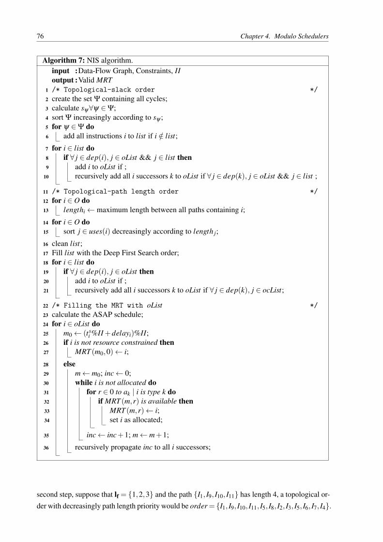
76 Chapter 4. Modulo Schedulers
Algorithm 7: NIS algorithm.input :Data-Flow Graph, Constraints, IIoutput :Valid MRT
1 /* Topological-slack order */2 create the set Ψ containing all cycles;3 calculate sψ∀ψ ∈Ψ;4 sort Ψ increasingly according to sψ ;5 for ψ ∈Ψ do6 add all instructions i to list if i /∈ list;
7 for i ∈ list do8 if ∀ j ∈ dep(i), j ∈ oList && j ∈ list then9 add i to oList if ;
10 recursively add all i successors k to oList if ∀ j ∈ dep(k), j ∈ oList && j ∈ list ;
11 /* Topological-path length order */12 for i ∈ O do13 lengthi← maximum length between all paths containing i;
14 for i ∈ O do15 sort j ∈ uses(i) decreasingly according to length j;
16 clean list;17 Fill list with the Deep First Search order;18 for i ∈ list do19 if ∀ j ∈ dep(i), j ∈ oList then20 add i to oList if ;21 recursively add all i successors k to oList if ∀ j ∈ dep(k), j ∈ ocList;
22 /* Filling the MRT with oList */23 calculate the ASAP schedule;24 for i ∈ oList do25 m0← (ts
i %II +delayi)%II;26 if i is not resource constrained then27 MRT (m0,0)← i;
28 else29 m← m0; inc← 0;30 while i is not allocated do31 for r ∈ 0 to ak | i is type k do32 if MRT (m,r) is available then33 MRT (m,r)← i;34 set i as allocated;
35 inc← inc+1; m← m+1;
36 recursively propagate inc to all i successors;
second step, suppose that lf = 1,2,3 and the path I1, I9, I10, I11 has length 4, a topological or-der with decreasingly path length priority would be order = I1, I9, I10, I11, I5, I8, I2, I3, I5, I6, I7, I4.

4.7. Modulo Schedulers Comparison 77
4.7. Modulo Schedulers ComparisonIn this section we present a detailed comparison between SDCS, ILPS, SMS, GAS, and
NIS.
Chart 5 presents a comparison between the SDCS, ILPS, GAS, and SMS. ILPS hasthe worse solving scalability, which also has the worse scaling with the loop size, n. Theoptimization problems solved by GAS and NIS have a better asymptotic scaling than the onessolved by SDCS, as GAS and NIS do not add allocation related constraints to its problems asSDCS does (Section 4.1).
Chart 5 – Comparison between the state-of-the-art and proposed modulo schedulers.
SDCS ILPS GAS NIS SMS
Problem type SDC ILP SDC SDC N/ASolve complexity Polynomial Exponential Polynomial Polynomial N/Aallocation related
constraintsgrows during
executionO(n2) 0 0 N/A
# Problems solved O(n2) 1 O(n) 2 N/AOptimal II guarantee no yes no no no
Optimal Latencyguarantee
no yes no no no
Source: Elaborated by the author.
The main SDCS source of inefficiency lies on its iterative heuristic search that triesto find a solution with a valid MRT, and on its incapability to prove infeasibility for a givenII. The ILPS main source of inefficiency lies on its quadratic scaling problem size, and itsexponential solver complexity. In contrast, GAS search solves a linear number of problems,achieving better complexity than SDCS. Furthermore, GAS problems are in the SDC form,maintaining a polynomial solving time. Finally, NIS solves a constant number of SDC problems,reaching further improvements in speed compared to GAS.
Concerning the quality of the achieved solution, SDCS does not guarantee latency or II
optimality due to its heuristic nature. If a solution cannot be found within a pre-allocated timebudget, the II is increased and a new search is performed. On contrary, ILPS guarantees bothlatency and II optimality, since the solver guarantees to find the optimal solution for the problem,for a given II, or declare infeasibility. GAS and NIS do not guarantee latency or II optimalitysince the GA may fail to find a feasible MRT before it reaches its stop criteria, and NIS cansimple create an infeasible MRT.
This section presents three different comparisons between the schedulers for a set ofbenchmarks presented in Section 4.7.1. First, Section 4.7.2 presents a speed-latency comparison,demonstrating the proposed schedules number of SDC solved problems reduction and the latencyand totalcycles impacts. Second, Section 4.7.3 presents results when loop unrolling is applied
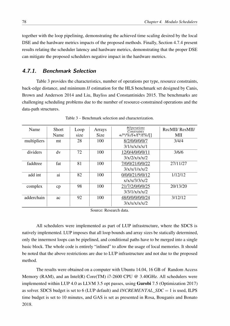
78 Chapter 4. Modulo Schedulers
together with the loop pipelining, demonstrating the achieved time scaling desired by the localDSE and the hardware metrics impacts of the proposed methods. Finally, Section 4.7.4 presentresults relating the scheduler latency and hardware metrics, demonstrating that the proper DSEcan mitigate the proposed schedulers negative impact in the hardware metrics.
4.7.1. Benchmark Selection
Table 3 provides the characteristics, number of operations per type, resource constraints,back-edge distance, and minimum II estimation for the HLS benchmark set designed by Canis,Brown and Anderson 2014 and Liu, Bayliss and Constantinides 2015. The benchmarks arechallenging scheduling problems due to the number of resource-constrained operations and thedata-path structures.
Table 3 – Benchmark selection and characterization.
Name ShortName
Loopsize
ArraysSize
#OperationsConstraints
+/*/%/f+/f*/f%/[]RecMII/ ResMII/
MIImultipliers mt 28 100 8/2/0/0/0/0/7
3/1/x/x/x/x/13/4/4
dividers dv 72 100 12/0/4/0/0/0/113/x/2/x/x/x/2
3/6/6
faddtree fat 81 100 7/0/0/21/0/0/223/x/x/1/x/x/2
27/11/27
add int ai 82 100 0/0/0/21/9/0/12x/x/x/3/3/x/2
1/12/12
complex cp 98 100 21/7/2/0/0/0/253/3/1/x/x/x/2
20/13/20
adderchain ac 92 100 48/0/0/0/0/0/243/x/x/x/x/x/2
3/12/12
Source: Research data.
All schedulers were implemented as part of LUP infrastructure, where the SDCS isnatively implemented. LUP imposes that all loop bounds and array sizes be statically determined,only the innermost loops can be pipelined, and conditional paths have to be merged into a singlebasic block. The whole code is entirely “inlined” to allow the usage of local memories. It shouldbe noted that the above restrictions are due to LUP infrastructure and not due to the proposedmethod.
The results were obtained on a computer with Ubuntu 14.04, 16 GB of Random AccessMemory (RAM), and an Intel(R) Core(TM) i7-2600 CPU @ 3.40GHz. All schedulers wereimplemented within LUP 4.0 as LLVM 3.5 opt passes, using Gurobi 7.5 (Optimization 2017)as solver. SDCS budget is set to 6 (LUP default) and INCREMENTAL_SDC = 1 is used, ILPStime budget is set to 10 minutes, and GAS is set as presented in Rosa, Bouganis and Bonato2018.

4.7. Modulo Schedulers Comparison 79
To evaluate the different schedulers effects on the hardware quality, all designs in thescaling tests have been implemented using Quartus II 16.1, targeting a Stratix V board, withOPTIMIZATION_TECHNIQUE=speed, auto_dsp_recognition off, dsp_block_balancing"logic elements", and max_balancing_dsp_blocks 0 to remove the usage of hardcoreDSP, avoiding influences in the Adaptive Logic Modules (ALMs) and Registers usage duringthis comparison.
4.7.2. Generated Schedules Comparison
Table 4 shows the number of problems solved for each benchmark. NIS solves only 2SDC problems per loop, while SDCS and GAS solve several problems. ILPS solves only oneILP problem per loop per candidate II. Table 4 also presents the reached II value, latency, totalnumber of cycles for loop completion, and total computation time for all schedulers. Table 4last column shows the row geomean normalized according to the SDCS geomean. All values inTable 4 are the average of 50 repetitions. The results for SDCS, ILPS, and NIS are integers sincethey are deterministic methods, while GAS has a random nature.
SDCS, ILPS, GAS, and NIS were able to find the minimum II for all benchmarks. SMSfails for all benchmarks apart from cp, for which it achieves a larger II than the other approaches.Further investigation on the failing cases reveals that SMS fails in its second heuristic (i.e. theone used to construct a schedule). This happens if back-edge instructions have conflicts in theMRT, making them be reallocated in a way that violates the back-edge constraints, forcing thealgorithm to stop and return a failure.
The obtained SMS results are not unexpected since list-based schedulers do not exploremultiple solutions, making them unable to handle loops with complex data-flows leading to nosolutions or to a schedule with larger IIs when compared with methods that explore multiplesolutions as shown in (Codina, Llosa and González 2002).
GAS and NIS achieve 20% and 16% worse latency than SDCS, making the total numberof cycles for loop completion to be affected by 5% and 1%, respectively. When consideringthe total computation time, NIS is 100× faster than SDCS, due to its constant number of SDCproblems solved. GAS is 3.17 times faster than SDCS. SMS is more than 100× faster than NISfor cp benchmark.
Even though results on Table 4 indicate that the larger latencies achieved by NIS andGAS have their impact amortized in the totalcycles, it is expected that pipelines with larger latencywill create deeper pipelines, which have larger register pressures, implying in need of moreregisters and multiplexers in the final hardware (Llosa et al. 2001).

80 Chapter 4. Modulo Schedulers
Table 4 – Performance and computation time comparison between the state-of-the-art and proposedmodulo schedulers (50 repetitions average).
Name mt dv fat ai cp ac geo. rate
#pr
oble
ms
solv
ed
SDCS 40 201 175 155 380 661 1ILPS 1 1 1 1 8 1 0.01GAS 17 71 174 62 120 95.64 0.37NIS 2 2 2 2 2 2 0.01SMS fail fail fail fail N/A fail N/A
Initi
atio
nin
terv
al
SDCS 4 6 27 12 20 12 1ILPS 4 6 27 12 20 12 1GAS 4 6 27 12 20 12 1NIS 4 6 27 12 20 12 1SMS fail fail fail fail 21 fail N/A
Lat
ency
(cyc
les)
SDCS 24 72 101 95 127 25 1ILPS 23 71 101 91 122 12 0.86GAS 26 .00 84 .00 118 .38 138 .73 155 .29 28 .00 1.20NIS 28 73 120 102 141 36 1.16SMS fail fail fail fail 121 fail N/A
Tota
l cyc
les(
103 ) SDCS 0.38 0.31 1.15 0.19 1.81 1.09 1
ILPS 0.38 0.31 1.15 0.19 1.80 1.08 0.99GAS 0.38 0.32 1.17 0.23 1.84 1.10 1.05NIS 0.38 0.31 1.17 0.20 1.82 1.10 1.01SMS fail fail fail fail 1,82 fail N/A
Tim
e(s
)
SDCS 1.34 12.35 17.08 18.23 35.61 32.92 1ILPS 1.79 3.42 e2 1.19 e3 1.14 e2 1.17 e3 1.13 e3 1.62 e3GAS 0.46 2.23 5.51 1.76 5.24 3.36 0.18NIS 0.07 0.08 0.07 0.06 0.12 0.11 0.01SMS fail fail fail fail 0.001 fail N/A
Source: Research data.
4.7.3. Scaling Comparison
To exemplify scalability, Figures 9 and 10 present the computation time and achieved II,respectively, as a function of the loop size when Loop Unrolling is applied (unrolled loopsize) before pipelining. Local memories are utilized to avoid memory bottlenecks, improvingperformance. The unroll factor is presented besides NIS marks. Missing points mean that thescheduler fails to find a schedule in a 1-hour budget. ILPS results are not presented for thisexperiment given its poor scalability.
Figure 9 shows how the NIS gain in speed increases with the loop size, what is

4.7. Modulo Schedulers Comparison 81
expected given its constant number of SDC problems solved. Figure 10 shows NIS and GAScan achieve better IIs than SDCS for large loops, indicating that NIS and GAS can improve thetotalcycles when compared to SDCS for very large and complex loops. Figures 9 and 10 missingpoints indicate that GAS and NIS can explore the solution space better than SDCS.
Figure 9 – Computation time in function of the unrolled loop size.
0 50 100 150 200 250 300
Unrolled loop size
10-4
10-2
100
102
104
time
(s)
mt
1 2 3 5
9
15
SDCSGASNIS
50 100 150 200 250 300 350
Unrolled loop size
10-4
10-2
100
102
104
time
(s)
dv
1 2
4 5
50 100 150 200 250 300 350 400 450 500
Unrolled loop size
10-4
10-2
100
102
104
time
(s)
fat
1 2 4 5 8
0 100 200 300 400 500 600 700 800 900
Unrolled loop size
10-4
10-2
100
102
104
time
(s)
ai
1 3 9 11
50 100 150 200 250 300 350 400 450
Unrolled loop size
10-4
10-2
100
102
104
time
(s)
cp
1
5
0 200 400 600 800 1000 1200
Unrolled loop size
10-4
10-2
100
102
104
time
(s)
ac
1 2 3 5 9 15
Source: Research data.
Figure 10 – II obtained as a function of the unrolled loop size.
0 50 100 150 200 250 300
Unrolled loop size
100
101
102
Initi
atio
n In
terv
al (
II)
mt
1
2
3
5
9
15SDCSGASNIS
50 100 150 200 250 300 350
Unrolled loop size
100
101
102
Initi
atio
n In
terv
al (
II)
dv
1
2
4 5
50 100 150 200 250 300 350 400 450 500
Unrolled loop size
101
102
103
Initi
atio
n In
terv
al (
II)
fat
1
2
45
8
0 100 200 300 400 500 600 700 800 900
Unrolled loop size
101
102
103
Initi
atio
n In
terv
al (
II)
ai
1
3
911
50 100 150 200 250 300 350 400 450
Unrolled loop size
20
30
40
50
60
Initi
atio
n In
terv
al (
II)
cp
1
5
0 200 400 600 800 1000 1200
Unrolled loop size
101
102
103
Initi
atio
n In
terv
al (
II)
ac
1
2
3
5
9
15
Source: Research data.
Figures 11, 12, and 13 present the number of ALM, registers usage and maximumfrequency achieved by the designs according to the unrolled loop size (10 repetitions average).The differences in Figures 11, 12, and 13 are explained by the fact that the schedule impactsstrongly the register pressure (Llosa et al. 1998), reflecting in the multiplexes network, maximumfrequency, and possible optimizations performed by the synthesis tool.
Figures 11 and 12 show that SDCS results in fewer hardware resources in most cases(when it can create a schedule), indicating a better register pressure than the other schedulers.NIS obtains results similar to SDCS in all benchmarks apart from dv, where its resources usage

82 Chapter 4. Modulo Schedulers
Figure 11 – ALM usage as a function of the unrolled loop size.
0 50 100 150 200 250 300
Unrolled loop size
0
0.5
1
1.5
2
2.5
3
ALM
s
104 mt
1 2
3
5
9
15SDCSGASNIS
50 100 150 200 250 300 350
Unrolled loop size
2000
4000
6000
8000
10000
12000
14000
ALM
s
dv
1
24
5
50 100 150 200 250 300 350 400 450 500
Unrolled loop size
2000
4000
6000
8000
10000
ALM
s
fat
12
4
5
8
0 100 200 300 400 500 600 700 800 900
Unrolled loop size
0
0.5
1
1.5
2
2.5
ALM
s
104 ai
1
3
9 11
50 100 150 200 250 300 350 400 450
Unrolled loop size
0.5
1
1.5
2
ALM
s
104 cp
1
5
0 200 400 600 800 1000 1200
Unrolled loop size
0
2000
4000
6000
8000
10000
12000
ALM
s
ac
1 2 3
5
9
15
Source: Research data.
Figure 12 – Registers usage as a function of the unrolled loop size.
0 50 100 150 200 250 300
Unrolled loop size
0
2000
4000
6000
8000
10000
12000
14000
Reg
s
mt
1 2
3 5
9
15SDCSGASNIS
50 100 150 200 250 300 350
Unrolled loop size
0.5
1
1.5
2
2.5
3
3.5
4
Reg
s
104 dv
1
24
5
50 100 150 200 250 300 350 400 450 500
Unrolled loop size
0.5
1
1.5
2
2.5
Reg
s
104 fat
12
45
8
0 100 200 300 400 500 600 700 800 900
Unrolled loop size
1
2
3
4
5
6
Reg
s
104 ai
1
3
9 11
50 100 150 200 250 300 350 400 450
Unrolled loop size
1
1.5
2
2.5
3
3.5
4
4.5
Reg
s
104 cp
1
5
0 200 400 600 800 1000 1200
Unrolled loop size
0
0.5
1
1.5
2
2.5
Reg
s
104 ac
1 2 3
5
9
15
Source: Research data.
is 2× larger than the other schedulers. This occurs because NIS does not optimize for latencyas much as GAS evolution or SDCS heuristic, resulting in a deeper pipeline which degradesincreasing hardware resources usage (Dai et al. 2017).
GAS presents worse or similar results to NIS in all benchmarks apart from dv, what isexplained by the fact that it quickly tries to find a valid and feasible solution, without optimizingthe register pressure. NIS ordering heuristics allocates instructions and its dependencies close toeach other, which reduces the register pressure (Llosa et al. 2001).
Figure 13 shows that NIS does not strongly impact the maximum frequency whencompared to SDCS, while it also shows the negative impact on the maximum frequency causedby the GAS larger register pressure.
Even though unrolling the loop prior to pipelining might reduce the number of clockcycles required to complete the loop execution, Figures 11 and 12 show that the negative impact

4.7. Modulo Schedulers Comparison 83
Figure 13 – Achieved maximum frequency as a function of the unrolled loop size.
0 50 100 150 200 250 300
Unrolled loop size
150
160
170
180
190
Fm
ax (
MH
z)
mt
1
2
3 5
9 15
SDCSGASNIS
50 100 150 200 250 300 350
Unrolled loop size
160
180
200
220
240
260
280
Fm
ax (
MH
z)
dv
1
2
4
5
50 100 150 200 250 300 350 400 450 500
Unrolled loop size
140
160
180
200
220
240
260
280
Fm
ax (
MH
z)
fat
1
2
4
5
8
0 100 200 300 400 500 600 700 800 900
Unrolled loop size
165
170
175
180
185
190
195
200
Fm
ax (
MH
z)
ai
1 3
9 11
50 100 150 200 250 300 350 400 450
Unrolled loop size
155
160
165
170
175
Fm
ax (
MH
z)
cp
1
5
0 200 400 600 800 1000 1200
Unrolled loop size
120
140
160
180
200
220
240
Fm
ax (
MH
z)
ac
1
2 3
5
9
15
Source: Research data.
in hardware resources and frequency can restrain the overall performance. Nevertheless, theusage of unrolling together with pipelining in this paper has its purpose of demonstrating the NISscalability and final hardware quality impact, as presented in Rosa, Bouganis and Bonato 2018.
4.7.4. Resources Constraints, Latency, and Hardware Metrics
In this section we explore the relation between schedule latency, resources constraintsand hardware resources usage, which is important to evaluate in which conditions GAS and NISdo not have a significant negative impact in the final hardware resources usage and how thisreflects in the local DSE.
In order to demonstrate the relation between schedule latency and hardware resourcesusage, we selected the benchmark dv as an example, which ALM and Registers usage stronglyaffected by the schedule latency according to empirical tests, and evaluate several schedules withdifferent latencies. An unroll factor of 2 is used to make the problem complex enough for theschedulers to return significantly different scheduler.
To create schedules with different latencies, ILPS, SDCS, GAS and NIS were used withthe configurations as described in Chart 6.
Chart 6 – Schedulers configurations to obtain schedules with different latencies.
ILP* ILPS without time budget, which provides the optimal solutionILP-10 ILPS with 10 minutes time budget;
GAS-0.5,-1,-2,-3 GAS with α = 0.5,1,2,3, respectivelyNIS NIS with the topological order presented in Algorithm 7
NIS-DFS NIS with a Deep-First Search topological orderSource: Elaborated by the author.

84 Chapter 4. Modulo Schedulers
Figures 14a and 14b present the ALM and registers usage in function of the latency foreach schedule. Even though the results in Table 4 show that the latency has a small impact in thetotalcycles, Figure 14 indicates that it might affect strongly the hardware resources used, whatmakes the overall optimization a more complex problem.
These effects indicate that NIS is more adequate for DSE early stages, where NIS fastercomputation time benefits the comparison of many different designs configurations, while amore robust scheduler, as ILPS, should be used in a fine optimization later stage of hardwaredevelopment.
Figure 14 – Hardware usage scaling with latency for benchmark dv.
(a) ALMs usage scaling with latency for bench-mark dv.
70 80 90 100 110 120 130 140 150 160
latency
5000
5500
6000
6500
AL
Ms
ILP*ILP-10
SDCS
GA-3GA-2GA-1
GA-0.5
NIS
NIS-DFS
(b) Register usage scaling with latency forbenchmark dv.
70 80 90 100 110 120 130 140 150 160
latency
1.5
1.55
1.6
1.65
1.7
1.75
1.8
1.85
1.9
1.95
Regs
104
ILP*ILP-10
SDCS
GA-3
GA-2GA-1GA-0.5
NIS
NIS-DFS
Source: Research data.
The correlation between latency and hardware resource usage observed in Figures 14a and14b does not imply that a smaller latency results in a smaller register pressure, as demonstratedby SDCS point which uses more resources while has larger latency than GAS-1, GAS-0.5, andNIS points.
It is important to notice that the resources constraints presented in Table 1 (the same asused by Canis, Brown and Anderson 2014 and Rosa, Bouganis and Bonato 2018), were fixedarbitrarily, implying that the extra resources usage due to schedules with larger latency in Figure14 is purely an overhead caused by the larger register pressure.
In this scenario, it is desirable to increase the resource constraints, which adds morecolumns to the MRT. The consequences of having more resources available are: a reduction ofconflicts during the scheduling, schedules with a shorter path (smaller latency), a possible II
reduction (for RecMII constrained benchmarks). Thus, increasing the resources constraints cansignificantly improve the overall number of cycles for loop completion However, to choose thebest number of resource constraints, a full resources constraints DSE must be performed.
To demonstrate that using the right set of resources constraints we can diminish the

4.7. Modulo Schedulers Comparison 85
schedulers hardware metrics impact we evaluate an exhaustive search over all combinationsof resources constraints using ILPS, SDCS, GAS, and NIS. Then, we calculate the Euclideandistance between the hardware metrics obtained with SDCS, GAS, and NIS and the hardwaremetrics obtained with ILPS.
Figure 15 presents the histograms showing how many designs there are aggregatedby the distance between the hardware metrics created using SDCS, GAS, and NIS and thehardware metrics created using ILPS (used as reference due its optimality) for the same resourcesconstraints configuration.
We do not present results for ai benchmark since its configuration space has more than100000 configurations, making unpractical to perform an exhaustive search.
Figure 15 shows that there are resources constraints configurations that result in smallhardware metrics impacts for all schedulers, indicating that the hardware metrics impacts ob-served in Figures 11 and 12 can be mitigated with proper resources constraints values definition.
Furthermore, Figure 15 gives us an idea about the negative hardware metrics probabilityfunction for each scheduler (supposing random configurations), which resembles a half-Gaussiandistribution. In this picture we can see how the standard deviation is higher for GAS and NIS.As such, the standard variation can be used as a metric to measure and compare the schedulersimpact in the hardware metrics.
The DSE can be accelerated by exploring the design space with NIS (or SDCS andGAS). The resulting Pareto-optimal solutions configurations can be used with ILPS to create anPareto-optimal approximation. To demonstrate the schedulers DSE impact in the final hardwaremetrics, we calculate the Pareto-optimal points for the exhaustive search using ILPS, whichwill serve as reference set. Then, we calculate Pareto-optimal points for the exhaustive searchusing SDCS, GAS, and NIS, and use the correspondent configurations to create designs usingILPS, resulting in the Pareto-optimal approximation for each scheduler. Finally, the two sets arecompared with the Average Distance from Reference Set (ADRS).
The ADRS is defined by Equation 4.6, where Γ = γ1, . . . ,γn, and Ω = ω1, . . . ,ωmare the reference points and approximated sets, respectively. In Equation 4.6, first the distancefrom a point in the reference set is calculated with all approximated set points. The minimalresult is accumulated for all reference set points and averaged. Thus, the closer ADRS is to0, the closer the Pareto curves are from each-other. Note that points repeated in the same setreduce the ADRS. Thus, we measure the ADRS only between unique points in the reference andapproximated sets.
ADRS(Γ,Ω) =1|Γ| ∑
γ∈Γ
minω∈Ω
[max
aω −aγ
aγ
,lω − lγ
lγ
](4.6)
Table 5 presents the ADRS reference set (using ILPS) and the approximated sets (using

86 Chapter 4. Modulo Schedulers
Figure 15 – Number of resources constraints configuration grouped by SDCS, GAS, and NIS hardwaremetrics distance from ILPS hardware metrics.
(a) mt.
10 11 12 13 13 14 15 16 16 17 18 180
5
10
15
20
25
30
Distance (x10)
# d
esig
ns
|ilp-sdc|
|ilp-gas|
|ilp-nis|
(b) dv.
11 14 16 19 21 24 26 29 31 33 36 380
20
40
60
80
100
120
140
Distance (x10)#
de
sig
ns
|ilp-sdc|
|ilp-gas|
|ilp-nis|
(c) fat.
15 17 19 21 23 26 28 30 32 34 36 380
50
100
150
200
Distance (x10)
# d
esig
ns
|ilp-sdc|
|ilp-gas|
|ilp-nis|
(d) cp.
10 11 12 12 13 14 14 15 16 16 17 180
500
1000
1500
2000
2500
Distance (x10)
# d
esig
ns
|ilp-sdc|
|ilp-gas|
|ilp-nis|
(e) ac.
12 15 17 20 23 26 29 32 34 37 40 430
5
10
15
20
25
30
Distance (x10)
# d
esig
ns
|ilp-sdc|
|ilp-gas|
|ilp-nis|
Source: Research data.
SDCS, GAS, and NIS), showing SDCS, GAS, and NIS impact the design space by less than 1%.The average distance is measured as avgDist = 100−geomeani∈benchmarks(100−ADRSi) sincethe geomean requires values greater than zero.

4.8. Final Remarks on Modulo Schedulers 87
Table 5 – ADRS (%) between ILPS Pareto-optimal solutions and SDCS, GAS, and NIS Pareto-optimalsolutions compiled with ILPS.
Benchmark mt dv fat cp ac avgDist
SDCS 0.000 0.957 0.597 0.322 0.000 0.376GAS 0.170 0.584 0.308 1.026 1.887 0.797NIS 1.481 1.505 0.704 0.467 0.804 0.993
Source: Research data.
Even though NIS results in an DSE ADRS 2.65× higher than SDCS, design spaceapproaches consider ADRS < 5% as low values, and ADRS < 1.7% as extremely low values(Schafer 2016). Thus, we can safely assert the NIS adequacy for speeding-up the DSE due to itsspeed-up compared to the other schedulers and the less than 1% impact in the final hardwareresources.
4.8. Final Remarks on Modulo SchedulersThe modulo scheduling methods in the literature are iterative approaches which dominate
the HLS time complexity, becoming a local DSE bottleneck. This bottleneck comes from theexcessive number of SDC problems solved by the methods, which were the acceleration target inthis chapter.
The proposed methods explore the explicit separation between the problem schedulingand allocation parts created by the proposed SDC formulation. As such the proposed GAS andNIS achieve an asymptotic reduction the in loop pipelining computation time, removing it as alocal DSE bottleneck.
Concerning the final implementation quality, the results demonstrate how latency andhardware resources usage relationship can impact the proposed methods usage. However we alsodemonstrate how this impact can be mitigated by defining proper resources constrains values,which also motivated the local DSE.


89
CHAPTER
5LOCAL DESIGN SPACE EXPLORATION
Recapping from Chapter 3, having a fast local DSE method has been identified as a keyto enable the local DSE, which was restricted by the loop pipelining computation time, especiallywhen applied alongside loop unrolling. Chapter 4 presented two new approaches for reducingthe loop pipelining scaling complexity, removing it as a DSE bottleneck. As such, we now focusthis thesis back on the local DSE acceleration.
Section 5.1 presents in-depth state-of-the-art approaches and analyses the literature toidentify its current gap, which show how the complex relationships between configuration anddesign spaces hurt the performance of the methods. Such analyses culminate in an individualdirectives study proposal, which allows mitigating the complex relationships between configura-tion and design spaces. As such, we propose to study loop pipelining, unrolling, and resourcesconstraints, which are three of the most impactful and common directives. The rest of this chapteris organized as follows:
Sections 5.2, 5.3, and 5.4 present proposed “white-box” approaches to explore theresources constraints, loop pipelining and unrolling directives, respectively. Finally, Section 5.5concludes this chapter.
5.1. Local DSE Inconsistencies Analysis
This section presents an in-depth analysis of the literature DSE methods aiming tohighlight their inconsistencies sources and strengths. These information can be incorporated intoour proposed approaches to obtain better results.
Recapping from Section 2.2, the local DSE methods can be categorized according to theirDSE speed-up mechanics as “Smart Selection”, “Modelling”, and “Architecture Fitting” methods,which allowed us to conclude that both “Smart Selection” and “Modelling” are required to achievepractical local DSE times without compromising the method with non-portable architectures.

90 Chapter 5. Local Design Space Exploration
“Architecture Fitting” methods will be spared from further analysis due to their portabilitiesrestrictions.
We separated the works presented on Section 2.2 in three groups, summarizing thespeed-up, results quality, and explored directives. The directives acronyms are presented onChart 7, and the three groups on Charts 8, 9, and 10.
Chart 7 – Directives acronyms for Charts 8, 9, and 10.
Acronym Directive
fi function inlinefb function branch typetb tree balancinglu loop unrollinglp loop pipelininglf loop foldlt loop tiling
Acronym Directive
rc resources constraintsmg memory portsmp array partitionmm array mappingmd memory duplicationmr memory reorganizationmc cache
Source: Elaborated by the author.
The works on Chart 8 are a continuous evolution of the Cyber compile DSE, focusingon reducing the number of evaluated designs, and also using ML techniques to create hardwaremetrics estimations. As such, these works present a progression being PMK (Schafer 2016) theone with better speed-up and smaller error.
The works on Chart 9 focus on creating hardware metrics estimations, which are usedto speed up the local DSE through an exhaustive search. The estimations depend on specificcomputation models, hardware architectures, compilers or tools, and can only model a sub-set ofHLS directives as loop unrolling, pipelining, data-flow and array partitioning (Ferretti, Ansaloniand Pozzi 2018). As such, these approaches fall out of this thesis scope alongside the hardwaremetrics estimations.
The works on Chart 10 use heuristics to reduce the number of evaluated designs, speeding-up de DSE. These works target miscellaneous compilers, and their portability is not constrainedto specific platforms or environments.
The approaches on Charts 8, 9, and 10 present as motivation for the ML methodsused the design space size non-trackability and how unpredictable are the relationships betweenconfiguration and design spaces. Such unpredictability is expected since many different directivesare put together to form the design space without considerations about the effects of each directivein the code, design, and configuration space.
Between the presented approaches, only PMK (Schafer 2016) treats directives differently.The directives are divided into three knobs. However, this division is motivated by the way thatthe directives are applied in the code, and not their design impacts.

5.1. Local DSE Inconsistencies Analysis 91
Chart 8 – Comparison Between Cyber compiler DSE methods.
Name Type Synthesis Speed-up Quality Over Direc-tives
ASA simulatedannealing
yes 3.80× +5% area,+8% latency
exhaustive
MLP GA + ML yes 2.04× 0.62%dominance
ASA
DC-ExpA heuristic yes 3.33× 0.88%dominance
ASA fi, fb,mm, lu, lf
PMK heuristic +swarm
yes 13× ADRS = 1.7% ASA
ERDSE GA + ML yes 9.8× ADRS = 10% ASASource: Elaborated by the author.
Chart 9 – Comparison Between estimation-only DSE methods (N/R - not reported).
Name Compiler Synthesis Speed-up Error Over Directives
PBDRO Rose yes N/R N/R N/R mcAladdin ILDJIT no 445× 6.5% error synthesis rc, lu, lp, mg
Lin-Analyzer LLVM no 123× 5.2% synthesis lu, lp, mpMPSeeker LLVM no 600× 12.8% synthesis lt, lu, lp, mpAutoAccel Merlin partial N/R 13.5% synthesis lp, mc, mrMKDSE SDCAccel N/R N/R N/R N/R lu, lp, mp
Source: Elaborated by the author.
Chart 10 – Comparison Between misc. DSE methods (N/R- not reported, N/A - not applicable).
Name Compiler Type Syn-thesis
Speed-up
Quality Over Directives
SDSE AUGH heuristic no 19× +8.8%latency
(Corre et al.2012)
rc, lu, mm
(AS)2 Vivado arch.matching
yes N/R N/R hand codeddesign
md, mp,mm, tb
PSCEFP N/R heuristic yes 2091× +3.3%latency
exhaustive PolyOpt
AO-DSE Vivado heuristic yes N/R N/A exhaustive fi, mp, lp,rc
SPIRIT Spark heuristic yes 200× ADRS =2%
ASA N/R
LBDSE Vivado lattice yes 132× ADRS =1%
exhaustive lu, fi, mg
Source: Elaborated by the author.

92 Chapter 5. Local Design Space Exploration
Such unpredictable relation between the configuration and design spaces should beexpected. Next, we present a list of unpredictability sources:
1. Directives act on different scopes. As an example, loop unrolling and pipelining targetspecific loops, while resources constraints affect the whole kernel code.
2. Local optimal directives are not optimal for the whole kernel. As an example, given akernel with two loops, the optimal resources constraints configuration for each loop are(probably) different, but if both loops are implemented within the same kernel, anotherconfiguration will (probably) be optimal.
3. Directives scope intersection. As an example, memory architecture optimizations arekernel-wide, but they affect loops implementations if the memories are used within theloop body.
4. Directives are non-orthogonal, meaning that the same design can be obtained with twodifferent sets of directives.
5. The directives application order impacts the final design implementation. By e.g., ifapplying loop interchange before unrolling and vice versa.
6. Treating different directives, in the same manner, creates false neighbourhood relations inthe design space.
Summarizing, many different optimizations are mixed-in, creating a complex relationshipbetween the configuration and design spaces, which is handled with “black-box” approaches,which are convenient due to its extendability and portability.
Going against such “black-box” approaches, we propose to consider each directiveindividually, analysing the relationships created between the configuration and design spaces.Such relations should not be unpredictable since all above-listed sources, apart from 2, come frommixing different directives. Furthermore, such analyses can unveil proper directive applicationorderings, handling the point 5.
As such, we expect that a DSE paradigm shift from “black-box” to a series of “white-box” approaches will enable to reach higher speed-ups and/or better accuracy in the local DSEmethods.
Directives that are not yet or cannot be analysed with “white-box” approaches can still beexplored with traditional “black-box” approaches separately, making the proposed paradigm shiftnot harmful to DSE approaches portability and extendability. Furthermore, interactions betweendifferent directives can be identified with a “white-box” analysis, allowing the exploration of suchrelations to improve the DSE. As such, for each directive that can be successfully analysed as a
5.1. Local DSE Inconsistencies Analysis 93
“white-box”, the configuration space is reduced combinatorially in size and an unpredictabilitysource is removed.
Next, we go through the state-of-the-art approaches, highlighting where their strengthsand inconsistencies are. Section 5.1.1 analyses approaches which take decisions based on designspace gradients, which is a common practice in many approaches on Charts 8 and 10. Section5.1.2 analyses the PMK, which presents the best results for the Cyber compiler. Finally, Section5.1.3 analyses the LBDSE, which Lattice nature presents advantages when compared to the otherheuristic based approaches.
5.1.1. Gradient-Pruning Based Approaches
Gradient-pruning based approaches are greedy heuristics that, given a DSE point, com-pute (compile, estimate, or measure) the hardware metrics for all its neighbours. Then, the pointresulting in a better gradient is chosen as the next point and the search iterates. SDSE, AO-DSE,and ERDSE are examples of such approaches.
This type of approach is suitable when all points in the design space form a typical Paretocurve, where reducing the resources constraints results in smaller and slower designs. However,reducing the resources constraints in a loop can have different results, as achieving the samedesign (if the resource is not a bottleneck), achieving a smaller and slower design (if the resourceis a bottleneck), or even resulting in a larger and slower design (due to increasing overhead,which will be discussed in Section 5.3).
Gradient-pruning based approaches make decisions based on weights given to eachdirective, which are defined by the hardware metrics gradient between the current design and itsneighbours. The gradient function can be written as Equation 5.1, where, dar and dtr are areaand time differences between the current design and the design after applying transformationT for each directive type r ∈R; Kcurr is a constant calculated from the current design metrics;gwT is a short-name for the global weight.
∇G = Kcurr
[dtda
](5.1)
In the literature, gwT is calculated for all directives. However, this leads to two criticalflaws.
The first flaw is that two configurations which vary only in one directive value are notnecessarily neighbours. E.g., a design implementation with and without pipelining result insignificantly different speeds and hardware resources usage, but they are considered neighboursby these approaches.
The second flaw appears when we consider Equation 5.1 and the possible da and dt
results, as the following scenarios:

94 Chapter 5. Local Design Space Exploration
1. da = 0 and dt = 0: ∇G = 00 ;
2. da = 0 and dt > 0: ∇G = ∞, and dn dominates dc;
3. da = 0 and dt < 0: ∇G = ∞, and dc dominates dn;
4. da > 0 and dt = 0: ∇G = 0, and dn dominates dc;
5. da < 0 and dt = 0: ∇G = 0, and dc dominates dn;
6. da > 0 and dt > 0: ∇G > 0, and dn dominates dc;
7. da < 0 and dt < 0: ∇G > 0, and dc dominates dn;
8. da|da| =−
dt|dt| : ∇G < 0, dn and dc trade-off area and speed.
In scenarios 2 and 3, we have that transformations create a better, and a worse design,respectively, however, ∇G cannot tell the difference between designs due to the singularity. Inscenarios 4 and 5, we have the same problem, but with ∇G = 0. In scenarios 6 and 7, we havethe same problem again, but ∇G cannot differ good and bad designs due to its maximizingnature and the division signal cancelling. Finally, in scenario 8, where different Pareto-points arereached, ∇G < 0, making transformation T not likely to be applied.
To reduce the second flaw inconsistencies, SPIRIT (Xydis et al. 2015) uses a signalmodel, which is more robust than Equation 5.1. The signal s[x] is defined as Equation 5.2, wheres[x] is a “signal” representing the area-time product, and x is the discrete vector formed by theresources constraints. As such, minimizing s[x] tends to the Pareto-optimal curve direction.
s[x] = Area(x)×Cycles(T ) (5.2)
However, minimizing s[x] does not imply in transversing all Pareto points. Figure 16presents a random space example and its k-Pareto curves on the left, and the signal s(x,y) = xy
for the respective curves on the right.
Figure 16 presents the first 5 Pareto curves over a set of random points and their respectivesignal strengths, demonstrating the general trend of approaching the Pareto optimal curve byminimizing s(x,y). Furthermore, s(x,y) has many peaks, meaning that minimizing s(x,y) doesnot imply in transversing a path between all Pareto-optimal points.
Furthermore, we can write the signal of the design obtained after applying a transforma-tion T as Equation 5.3.

5.1. Local DSE Inconsistencies Analysis 95
Figure 16 – Set of points and k-Pareto curves on the right. Corresponding signal s(x) on the left.
0 0.1 0.2 0.3 0.4 0.5 0.6 0.7 0.8 0.9 1
x
0
0.1
0.2
0.3
0.4
0.5
0.6
0.7
0.8
0.9
1
y
0 0.1 0.2 0.3 0.4 0.5 0.6 0.7 0.8 0.9 1
x
0
0.01
0.02
0.03
0.04
0.05
0.06
0.07
0.08
s(x
, y)
k=1
k=2
k=3
k=4
k=5
Source: Elaborated by the author.
s[dn] = Area(dn)×Cycles(dn)
= (Area(dc)−da)× (Cycles(dc)−dt)
= s[dc]−Area(xc)dt−Cycles(xc)da+dadt (5.3)
Here we can see that, in scenario 1 the signal does not change, as expected. In scenarios2, 4, and 6, s[xT ] increases, and in scenarios 3, 5, and 7, s[xT ] decreases, being consistent indifferentiating better and worse points. However, in scenario 8 we again consider Area(xc)> da
and Cycles(xc)> dt, s[xT ] is negative, and instead of reaching a possible new Pareto point, thes[xT ]< 0 inconsistently interprets the point as a worse configuration.
Scenario 8 is the most important scenario since it is the one which represents thefinding of a new point “possibly” in the same Pareto curve. Furthermore, gradient-pruning basedapproaches also suffer from local traps in the design space.
5.1.2. The Probabilistic Approach
The PMK probabilistic model (Schafer 2016) results from the Cyber compiler DSEevolution, which is detailed in this section, alongside with its steps discussions and strengthshighlighted. The PMK main idea is to divide the directives into three knobs, the local knob,#FUs, and global knob (already discussed in Section 2.2) depending on how they are applied.
The approach is divided in two parts. First, an Ant Colony Optimization (ACO) (Wang2007) is used to explore the local knob. Each configuration is synthesized with minimum andmaximum #FUs (Dmin and Dmax, respectively), which gives an idea about the design space regioncontaining all designs generated by varying the number of FU. Then the ACO is performedreturning a set of dominant local knob configurations to the second step.
Second, the probabilistic model is used to explore the #FUs knob, where each local knobconfiguration is associated with a probability function proportional to the area between Dmin and

96 Chapter 5. Local Design Space Exploration
Dmax. The probability function sets large areas with high exploration priority, and overlappingareas low with priority. Finally, to explore the designs in each area, the resources constraintsare varied from Dmax to Dmin by 10% intervals, which has empirically shown to provide a goodbalance between exploration speed and results quality for the presented tests.
We refrain from presenting PMK full algorithms for conciseness reasons since we areinterested only in the above observations.
This is the only approach in the literature that does not analyze all directives in the samemanner. However, directives are classified according to their application scope and method,resulting in a “black-box” approach. Furthermore, PMK uses a simple linear distribution toexplore the #FUs, which can lead to sub-optimal results since bottleneck balancing is notconsidered. However, it has shown to be efficient at avoiding local-optimal plateaus.
The promising results obtained by PMK indicate that a clear separation between directiveshelp to improve the DSE methods performance, corroborating with our “white-box” paradigmproposition.
5.1.3. The Lattice-Based Approach
The LBDSE lattice-based approach (Ferretti, Ansaloni and Pozzi 2018) is the firstto observe relationships between the design and configuration spaces. Through a PrincipalComponent Analysis (PCA), it is empirically observed that Pareto-optimal points cluster in theconfiguration space, while they are spread in the design space. To explore such characteristic, theconfiguration points are normalized, and the lattice-based exploration presented in Algorithm 8is realized over the design space.
Algorithm 8 first uses an U-distribution to select random configuration points (line 1),which are synthesized (line 2). This distribution makes that designs with more extreme valuesare more likely to be chosen. From this distribution, m individuals are sampled in the algorithminitialization part.
In the iterative part, the Pareto optimal points (between the points that have already beenvisited) are selected and have their σ -neighbours synthesized (lines 7 to 9). The selection andsynthesis process is iterated until no new Pareto optimal points are found, or a budget is exceeded(lines 13 to 15). Finally, all compiled designs configurations and results are returned (lines 5, 6,10, 12, and 16).
As such, LBDSE has two parameters to control the number compiled designs and theresults quality trade-off: m, which controls the initial sampling number; and σ , which controlsthe how many neighbours will be explored per point. These parameters must be adjusted for thetarget compiler and directive sets.
By considering and exploring that Pareto-optimal points cluster in the configuration

5.2. Stand-alone Resources Constraints Exploration 97
Algorithm 8: Lattice-based DSE algorithm.input :List of directives and possible valuesoutput :List of configurations and metrics
1 con f igs← m U-distribution random configurations;2 designs← synthesize and annotate area and cycles;3 nextCon f igs← pareto(con f igs,designs);4 count← size(con f igs);5 compiledCon f igs← con f igs;6 compileDesigns← designs;7 do8 con f igs← σ -neighbours of nextCon f igs;9 designs← synthesize and annotate area and cycles;
10 nextCon f igs← pareto(con f igs,designs);11 append con f igs to compiledCon f igs;12 append designs to compileDesigns;13 if count ≥ budget then14 break;
15 while nextCon f igs = /0;16 return compiledCon f igs and compileDesigns;
space, LBDSE is the first approach that explores the relationships between the configurationand design spaces in order to realize a local DSE speed-up method. This strongly motivates ourproposed approach of studying and evaluating such relations for each directive individually.
The major flaw in this approach lies within its U-shaped distribution initialization, whichtends to create fast-and-large and slow-and-small designs only, leaving gaps that balance the areaand number of clock cycles reduction susceptible to local plateau traps.
5.2. Stand-alone Resources Constraints Exploration
Resources constraints are the most basic type of directives, which control how manyfunctional units the design will implement, influencing area and speed (number of clock cycles)trade-off. However, this is not a straightforward relation since the resources constraints affect theinstructions schedule, which affects the number of clock cycles and hardware resources usage.
Using the Section 5.1 observations, we propose two new approaches for exploring theresources constraints, the first explores neighbour relations in the configuration and designspaces, and the second is an LBDSE improvement, both aim to reduce the number of evaluateddesigns and while keeping comparable accuracy.

98 Chapter 5. Local Design Space Exploration
5.2.1. Proposed Approach
The main idea behind the proposed approach is that Pareto points will be close to eachother if they are in the same design space plateau. However, different plateaus will vary inproportions between the resources constraints. As such, we proposed a neighbour search (as usedby LBDSE) until a plateau is found, then we perform the 10% reduction rule (used by PMK) toescape such local optima traps.
The proposed approach tries to find a path between two extreme points, one with noresources constraints, and another with FU constrained to 1. By evaluating points in this path, weexpect to find Pareto-optimal designs in the same fashion as the gradient-pruned based searches.Moreover, by evaluating a whole path connecting these points, we expect to reach transversethrough plateaus containing Pareto-optimal solutions.
We define the Design Space Graph (DSG) as a graph connecting the two extreme pointsas follows:
Give the set of resources to be constrained K = add,mult,div, . . ., each one withmaximum values ak defined by the number of instructions in the code, we define the resourcesconstraints graph R = N,E, where each node n ∈ N is a unique array e = e1,e2, . . . with1≤ ei ≤ ai, and each edge ∃ e = ni,n j if, and only if |n1,n2|= 1. If ∃ e = ni,n j, we say thatni and n j are neighbours. the graph has the nodes nmax = a1,a2, . . . ,a|K| and n1 = 1,1, . . . ,1.
Figure 17 presents a DSG example with |K|= 3 and nmax = 3,2,2. Note that the graph
has |N|=|K|
∏i∈1
ak nodes, representing the whole design space formed by the resources constraints.
Figure 17 – Example of resources constraints design space graph.
n_max = [3, 2, 2]
[2, 2, 2]
[3, 1, 2]
[3, 2, 1]
[1, 2, 2]
[2, 2, 1]
[2, 1, 2]
[3, 1, 1]
[1, 1, 2]
[1, 2, 1]
[2, 1, 1]
n_1 = [1, 1, 1]
Source: Elaborated by the author.
Each unique resources constraints configuration is a DSG node connected to all itsneighbours. The resources constraints DSE objective is to find a DSG path between the pointsnmax and n1 visiting the maximum number of Pareto points as possible.
The DSG transversal is made by evaluating the current point neighbours to select the

5.2. Stand-alone Resources Constraints Exploration 99
next one, similarly to Gradient Pruning approaches, and to use a set of conditionals varying ifda,dt=,>,<0, to realize if neighbour points are better, worse, or different Pareto points. Byusing the conditionals, we avoid the inconsistencies presented by the signal and gradient models,at the cost os 8 if-then-else statements.
To avoid local plateaus, we include the 10% variation rule from Schafer 2016, which willgenerate nodes with different resource constraints proportions. As demonstrated, these pointshave a higher probability of belonging to different plateaus.
Algorithm 9 presents the proposed DSG Path-based DSE (PBDSE) approach. First,nmax, n1 and di f f 10 constants are defined, along with queues to annotate which designs werecompiled and discarded (lines 1 to 6), and a queue to save which are the possible configurationsto be searched next (line 7).
At this point, it is important to notice that the hardware resources usage and clockcycles can be obtained by synthesis, simulation, or estimation. We use hardware elaborationand behavioural simulation to obtain the hardware metrics, which is a relatively fast option,has good accuracy and is portable, since it depends only on the synthesis tools and not on theHLS environment. However, any method to obtain the hardware metrics can be used instead ofcompilation (lines 8 and 17).
The approach iterative part (lines 10 to 31) starts with search queue being popped toget the design which will be explored together with its neighbours which are created using thefunction presented in Algorithm 10 (lines 11 and 13). Algorithm 10 returns all neighbours thatwere not explored or discarded by the compilation function presented in Algorithm 11.
In case neighbours are found (lines 15 to 20), they are compiled using the Algorithm 11(line 16), which iteratively compiles the neighbourhood designs until a dominant design or onewith the same hardware metrics is found. As such, Algorithm 11 compiles only a neighbourssubset. Then, dominated designs are excluded from the search using the 8 conditions presentedin Section 5.1.1 (lines 17 to 20). The search queue is updated by removing dominated points itmay contain (line 21). Removing dominated points from the search queue reduces the number ofevaluated designs forcing the algorithm only to visit the most promising points.
If no neighbours were found, which can happen in local-optimal plateaus, we apply thePMK 10% reduction rule iteratively until we achieve a configuration different from n1 that hasnot been compiled or discarded is found (lines 23 to 30).
Algorithm 10 presents the function to get neighbours used by Algorithm 9, where a newconfiguration is created by reducing 1 from each resource constraint in the input configurationindependently (lines 2 to 6), regarding to not reduce the constraints to less than 1 (lines 4).
Algorithm 11 presents the function to compile the neighbours from a given design, whichiteratively compiles one design at a time (lines 2 to 10). In case a neighbour is found to dominateor to result in the same hardware metrics as the current design, the compilation stops, and the

100 Chapter 5. Local Design Space Exploration
Algorithm 9: Proposed Path-based DSE algorithm 9.input :Data-Flow Graph (DFG)output :Resources constraints and evaluated points metrics
1 nmax← maximum resources;2 n1← ones vector;3 di f f 10← ⌈0.1* (nmax−n1)⌉;4 currConstr← nmax;5 compiled← [nmax];6 discarded← /0;7 searchQueue← nmax;8 compile nmax;9 currMetrics← nmax metrics;
10 do11 curr← searchQueue.pop();12 currMetrics← curr metrics;13 neighbors← getNeighbors(curr) ;14 /* do not add points which are dominated by curr */15 if neighbors = /0 then16 nMetrics← compileNeighbors(curr);17 calculate da and dt for each neighbour;18 for n ∈ neighbors do19 if (da > 0 || dt > 0) || (da == 0 && dt == 0) then20 searchQueue.insert(n);
21 searchQueue← pareto(searchQueue);22 /* apply the 10% rules */23 if searchQueue == /0 && n1 /∈ compiled then24 newCon f ig← curr−di f f 10;25 change to 1 where newCon f ig≤ 0;26 while
newCon f ig ∈ compiled || newCon f ig ∈ discarded && newCon f ig = n1 do27 newCon f ig← curr−di f f 10;28 change to 1 where newCon f ig≤ 0;
29 searchQueue.insert(newCon f ig);
30 while searchQueue = /0;
un-compiled designs are discarded (lines 7 to 10).
The proposed PBDSE approach (Algorithm 9) handles the flaws observed in the gradient-pruning based approaches and PMK. The flaw presented in LBDSE can be handled by a simpleextension of Algorithm 8. The idea behind this extension is to use the PBDSE results instead ofthe U-shaped distribution in Algorithm 8. As such, with an initialization closer to the Pareto, wecan avoid the local plateaus problems and speed-up the convergence.
Algorithm 12 presents the proposed expansion in the input line list and lines 1 to 4 whichshould substitute line 1 in Algorithm 8. This combination will be referred to as Path Seed

5.2. Stand-alone Resources Constraints Exploration 101
Algorithm 10: getNeighbors() function used bt Algorithm 9.input :Design configuration curr.output :Neighbors configurations rSet.
1 rSet← /0;2 for a ∈ curr do3 newCon f ig← curr;4 newCon f ig(a)← max(newCon f ig(a),1);5 if newcon f ig /∈ compiled && newcon f ig /∈ discarded then6 rSet.insert(newCon f ig);
Algorithm 11: compileNeighbors() function used bt Algorithm 9.input :Current design curr and its list of neighbours neighbors.output :Metrics for the compiled designs rMetrics.
1 cp← /0;2 for n ∈ neighbors do3 compile n;4 calculate da and dt;5 add n to cp;6 if da≥ 0 && dt ≥ 0 then7 break;
8 /* compiled and discarded queues in Algorithm 9. */9 append cp to compiled;
10 append neighbors/cp to discarded;
Lattice-Based DSE (P+LBDSE).
Algorithm 12: Lattice-based DSE algorithm accepting seed configurations.input :List of directives and possible values, seeds
1 if seeds = /0 then2 con f igs← seeds
3 else4 con f igs← m U-distribution random configurations;
5.2.2. Resource Constraints Exploration Results
To evaluate how close from the estimated Pareto curve are from the real Pareto curve,we calculate the ADRS (Equation 4.6) between the exhaustive search Pareto-optimal points(reference set) and the PBDSE, LBDSE, and P+LBDSE (approximate sets) Pareto-optimal points;Note that a fair comparison with the literature is not trivial since other approaches consider moredirectives than just the resource constraints and also the whole code is targeted by the DSE,while we focus on loops only. Thus, we do not present results for PMK and gradient-pruningbased approaches.

102 Chapter 5. Local Design Space Exploration
Table 6 presents the number of synthesized configurations for PBDSE, LBDSE andP+LBDSE, without loop pipelining (“No-pipe” for short) and using NIS and ILPS to createloop pipelines. Empirical tests have shown that (m,σ) = (0.1,0.25) are adequate to explore theconfiguration space formed by the resources constraints in our environment. The experimentspresented in Ferretti, Ansaloni and Pozzi 2018, Ferretti, Ansaloni and Pozzi 2018 use (m,σ)≥(0.2,0.5) to achieve an ADRS < 1%. The necessity of a larger σ is caused by a more complexand unpredictable design space created by different optimizations, while our tests consider onlythe resource constraints.
Table 6 – Number of compiled configurations and ADRS obtained by PBDSE (P), LBDSE (L), andP+LBDSE (50 repetitions average).
No-pipe NIS ILPSP L P+L P L P+L P L P+L
# configs
mt 12 6.00 12 11 6.00 11 11 6.00 11dv 30 31.92 32 21 28.68 23 27 33.30 32fat 36 137.88 114 35 105.16 79 40 101.16 111cp 35 842.30 79 86 2011.3 473 74 1180.30 352ac 35 46 52 28 32.60 49 30 34.22 55
ADRS
mt 0 0.99 0 0 0.65 0 0 0.63 0dv 0.095 0.011 0.095 0.86 0.82 0.86 0.41 0.38 0.41fat 0.24 0.023 0.22 0.22 0.46 0.22 0.20 0.14 0.18cp 0.16 0.0036 0.15 0.38 0 0.033 0.30 0.031 0.11ac 0 0 0 0 0.38 0 0 0 0
Source: Research data.
First, we can not notice any substantial difference between using NIS and ILPS in Table6, allowing to save computation time when compared with other module schedulers.
Table 7 shows the design space size and computation time for the exhaustive searchrealized to obtain the Pareto-optimal points. Note that the hours-scale DSE times are due tothe usage elaboration and simulation to obtain the hardware metrics, and the time differencesbetween ILPS and NIS should be more pronounced were faster estimation methods used. It isimportant to notice that loops without pipeline are scheduled as sequential code, by solving aconstant number of SDC problems (Canis et al. 2013), resulting in computation times comparableto NIS, which also solves a constant number of SDC problems.
As such, the NIS small ADRS and large time savings corroborate with its adequacy forexploring design spaces in the early phases of a project.
Table 6, also shows that the ADRS is always larger when loop pipelining is used, what iscaused since the pipelined design space has a clustering effect and creates larger overheads thanthe non-pipelined design space (will be explored in details in Section 5.3).
Table 6 shows that, for all benchmarks apart from mt, the PBDSE evaluates less points

5.3. Loop Pipelining Exploration 103
Table 7 – Design space size and full exhaustive DSE time without pipeline and with NIS and ILPS tocreate pipelines.
mt dv fat cp ac
Design Space Size 30 128 168 3920 48
time (hours)No-pipe 1.5 6.4 6.4 84 2.4
NIS 1.6 6.5 6.5 98 2.5ILPS 1.9 8.3 8.4 251 10,1
Source: Research data.
than LBDSE. However, PBDSE reaches the ADRS < 1% condition for which LBDSE is tunedto. P+LBDSE number of evaluated designs include the designs evaluated by PBDSE, and whencompared to LBDSE show little improvement for all benchmarks apart from cp, indicating thatthe benefits of seeding the LBDSE are more significant for larger and more complex designs.
Furthermore, P+LBDSE can not degrade the PBDSE ADRS, making the exploration tobe another option to balance the DSE speed-up and accuracy.
5.3. Loop Pipelining ExplorationPipelining is one of the most important optimizations since it improves the throughput in
exchange for increasing the hardware resources usage. This section presents studies on relationsbetween the design space formed by the FU without and with loop pipelining, which allowsto perform the DSE in one space and use its information to quickly explore the second one,reducing the number of evaluated designs. As such, we first analyse the loop pipelining effectson the design space, which allow us to propose a practical measure of similarity between thedesign spaces without and with pipelining. Finally, we propose a new “white-box” approach toexplore both design spaces efficiently.
5.3.1. Loop Pipelining Effects on the Design Space
The goal of this section is to explicitly analyse the loop pipelining effects in the designspace formed by the number of FU. To do so, Figure 18 presents the complete FU design spacefor the benchmarks used in Canis, Brown and Anderson 2014 without loop pipelining and whenNIS and ILPS are used to create the pipelines.
As expected, Figure 18 shows that all points in the design space have their number ofclock cycles reduced when pipelining is applied, while the hardware resources usage increases.We also can observe that NIS points use more hardware resources than ILPS, which is expectedaccording to Section 4.7.4. Furthermore, we can observe that the pipelined design spaces areclustered in the cycles-axis. This clustering happens since the II is the major contribution forpipelined designs cycles, which varies less than the loop latency.
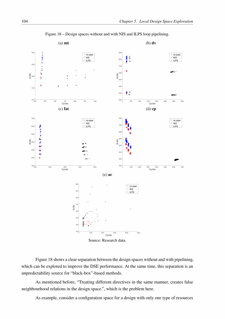
104 Chapter 5. Local Design Space Exploration
Figure 18 – Design spaces without and with NIS and ILPS loop pipelining.
(a) mt
400 500 600 700 800 900 10001700
1750
1800
1850
1900
Cycles
AL
Ms
no-pipe
NIS
ILPS
(b) dv
0 500 1000 1500 2000 2500 3000 35002000
3000
4000
5000
6000
7000
8000
9000
Cycles
AL
Ms
no-pipe
NIS
ILPS
(c) fat
1000 2000 3000 4000 50001000
2000
3000
4000
5000
6000
7000
Cycles
AL
Ms
no-pipe
NIS
ILPS
(d) cp
0 1000 2000 3000 4000 5000 6000 70004000
4500
5000
5500
6000
6500
7000
7500
Cycles
AL
Ms
no-pipe
NIS
ILPS
(e) ac
0 1000 2000 3000 4000 5000300
400
500
600
700
800
900
1000
Cycles
AL
Ms
no-pipe
NIS
ILPS
Source: Research data.
Figure 18 shows a clear separation between the design spaces without and with pipelining,which can be explored to improve the DSE performance. At the same time, this separation is anunpredictability source for “black-box”-based methods.
As mentioned before, “Treating different directives in the same manner, creates falseneighbourhood relations in the design space.”, which is the problem here.
As example, consider a configuration space for a design with only one type of resources

5.3. Loop Pipelining Exploration 105
and two instructions Cinit = c1 = [1],c2 = [2]. The literature DSE methods add a Booleanvariable to represent when loop pipelining is on or off (let it be represented by 1 and 0respectively), resulting in the new configuration space: Cpipe = c1 = [1,0],c2 = [2,0],c3 =
[1,1],c4 = [2,1].
In this case, points c1 and c3 are neighbours (same for c3 and c4). However, as demon-strated by Figure 18, points c1 and c3 are probably not close from each other in the combineddesign space Cpipe. This discrepancy is an uncertainty source while relating the configurationand design spaces, which prejudices typical DSE algorithms.
To avoid this situation, the straightforward idea is to explore both design spaces separatelyand merge the resulting Pareto estimations for each space to form a final estimation. As such,it solves the unpredictability source and achieves more accurate results. However, in the nextsection, we will explore relationships between the design spaces without and with pipelining.The unveiling of such relations can allow avoiding exploring both design spaces thoroughly as inthe straightforward approach, achieving further speed-ups.
5.3.2. Practical Measure to Compare Design Spaces
This section proposes a practical measure that can be used to highlight relationshipsbetween design spaces without and with pipelining. The indication of similarities between thedesign spaces can be used to speed-up the DSE with the approach proposed in Section 5.3.3.
Let O be the set of DFG instructions with size n = |O|; let li=1,l...,k be the set composedby the instructions type; and let ak ≥ 1 be the number of instructions of type k. A configuration isrepresented by the vector ci, which element represent the resources constraints for resource type
k. As such, the total number of possible configurations is p =k
∏i=1
ai. The set of all configurations
is defined as:
C =
ci =
c1
i...
cki
∣∣∣∣∣∣∣∣1≤ c j
i ≤ ak ∀ i = 1, . . . , p, j = 1, . . . ,k
(5.4)
For each compiled design using configuration ci, we obtain a set of metrics, representedby an m-array, such as m ≥ 2, since we measure the number of clock cycles for the loopcompletion and at least one type of hardware resources usage. Thus, we write the set of metricsfor the compiled designs without pipelining as:
B =
bi =
b1
i...
bmi
∣∣∣∣∣∣∣∣1≤ b j
i ∀ i = 1, . . . , p, j = 1, . . . ,m
(5.5)

106 Chapter 5. Local Design Space Exploration
Similarly, the set of metrics for the compiled designs with pipelining is written as:
A =
ai =
a1
i...
ami
∣∣∣∣∣∣∣∣1≤ a j
i ∀ i = 1, . . . , p, j = 1, . . . ,m
(5.6)
Let also f ,g : C→ B,A be two surjective functions such as bi = f (ci) and ai = g(ci),respectively. As this point, we want to relate the spaces B and A to speculate if there is a relationbetween Pareto points in B and A. The motivation behind this is, the closer the B Pareto pointsare from the ones in A, less exploration is necessary to find the A Pareto points (and vice-versa).
We propose a measure to estimate how close A and B are from each other. As such,when applied over a set of representative benchmarks, the measure gives an idea about how thedesign spaces created by a compiler behave. The measure can be used with any number of pointsevaluated with and without loop pipelining and represents the value for a given benchmark,which opens the possibility to be used dynamically. However, this is not explored in this thesis.
The measure is constructed based on the relative position between pairs of points in bothspaces. Formally, we define that two configurations (ci1,ci2) maintain their relative positions inspaces B and A if the relations b j
i1 (< | > | =) b ji2⇔ a j
i1 (< | > | =) a ji2 ∀ j = 1, . . . ,m.
Consider the 2−D example presented in Figure 19, where Figure 19a presents two pointsin a reference space, Figure 19b presents two correspondent points in another space that maintainthe same relative position as in Figure 19a, while Figures 19c, 19d, and 19e present points thatdo not maintain the same relative position as in Figure 19a.
Figure 19 – Relative position in two different sets example. B in orange and A in green.
(a) Referencepoints.
(b) Samerelativepositions.
(c) Differentrelativepositions.
(d) Differentrelativepositions.
(e) Differentrelativepositions.
Source: Elaborated by the author.
We define the Set Relative Position Distance (SRPD), which is an average based measurethat indicates how many points in two sets maintain their relative positions, as Equation 5.7. Theterm (ak
i −akj)(b
ki −bk
j)≥ 0 is a logical comparison, returning 1 when it is true and 0 otherwise.
SRPD =2
p(p−1)
p
∑i=1
p
∑j=i+1
m
∏k=1
[(ak
i −akj)(b
ki −bk
j)≥ 0]
(5.7)

5.3. Loop Pipelining Exploration 107
Equation 5.7 measures the average number of pairs-of-points that maintain their relativepositions in two spaces A and B. For each distinct pair of points i and j, 1 is added to the measureif their relative positions hold in all dimensions, represented by the ∏ term. Then, the number ofpairs that hold their relative positions is summed up before being averaged by the term 2
p(p−1) .Note that the logical comparison ≥ means that, if the pair of points coincide in both A or B, weconsider that the points maintain their relative positions.
Equation 5.7 converges to 1 or 0 if all pairs-of-points maintain or not their relativepositions, respectively. This is a useful tool that can be used to empirically study and compare thedesign spaces with and without pipelining (varying the resources constraints) for any compileror set of codes. By defining and elaborating the design space for a set of benchmarks with andwithout loop pipelining, SRPD can be calculated. If SRPD≈ 1 for all benchmarks, then one canconclude that the design spaces are similar and only one needs to be effectively explored.
Table 8 presents the SRPD evaluation over the loop pipelining benchmarks used in Sec-tion 4, and the SRPD considering only the cycles and ALMs SRPD components independently.
Table 8 – SRPD for design spaces without and with NIS and ILPS loop pipelining.
SRPD Scheduler ac mt dv fat cp
totalILPS 0.878 0.729 0.488 0.547 0.232NIS 0.922 0.837 0.502 0.689 0.232
cyclesILPS 0.937 0.978 0.923 0.937 0.897NIS 0.937 0.978 0.937 0.963 0.799
ALMsILPS 0.923 0.849 0.674 0.684 0.448NIS 0.924 0.849 0.536 0.723 0.497
Source: Research data.
Table 8 shows that SRPD is small for the compiler used (LUP), however, the independenthardware metrics shows that the SRPD cycles component is close to 1, and the small SRPD iscaused by the small SRPD ALM component. Each SRPD metric component shows the designslikelihood to keep their relative position for that metric. As such, we can conclude that a fasterdesign in a space without pipeline will probably result in a faster design when pipelined.
We expect that the low SRPD ALM component value is due to designs fluctuatingin-between the small local clusters in Figure 18; however, this subject needs further evaluation.
Furthermore, Table 8 shows no significant difference regarding the loop pipeliningmethod used, what corroborates with the NIS usage during the project DSE phase.
5.3.3. Proposed Approach for Exploring Loop Pipelines
In this section presents a new method to explore the design space formed by the numberof FU and loop pipelining based on the design spaces separation and SRPD results.

108 Chapter 5. Local Design Space Exploration
The literature DSE approaches combine the configuration space considering the looppipelining turned on and off with the number of FU, resulting in an effective twice as largeconfiguration space, on which the DSE is performed. This flow is presented in Figure 20. We willuse the terminology B
⋃A to refer to the combined design space approach used in the literature.
Figure 20 – Typical DSE flow considering resources constraints and loop pipelining.
Config. Space
Turn Loop
Pipeline on
Turn Loop
Pipeline off
New Config. Space fast DSE Explored Points Find Pareto
Selected Design Points
Source: Elaborated by the author.
As noted in Section 5.3.1 exploring B and A separately and merging the results is astraightforward manner to increase the exploration precision. This flow is presented in Figure 21.We will use the terminology B+A to refer to the proposed separate design space exploration.
Figure 21 – Proposed DSE pipeline independent flow considering resources constraints.
Config. Space
Turn Loop
Pipeline on
Turn Loop
Pipeline offfast DSE Explored Points Find Pareto
fast DSE Explored Points Find Pareto
Selected Design Points
Source: Elaborated by the author.
Next, we present another approach aiming to achieve further DSE improvements byexploring the SRPD observations presented in Section 5.3.2.
The main idea of this second proposed approach is to perform the DSE in space B anduse its results as seeds to explore the space A with P+LBDSE. The reasoning for this is thatsince the points maintain their relative positions in the cycles axes, the Pareto points from B
will contain a sample of each II cluster observed in Figure 18. Furthermore, the SRPD ALMcomponent indicates that more than half of the pairs-of-points maintain their relative positions inthis direction, indicating a more than 50% chance of B Pareto points to be also A Pareto points.As such, we expect to diminish A exploration using the fact that B Pareto points should be closeto A Pareto points.

5.3. Loop Pipelining Exploration 109
We choose to use B results to seed A since the DSE in B results in a generally smallerADRS, as presented in Table 6. Empirical results also have shown that the “B seeds A” achievesbetter results than vice-versa. The proposed seeding-based flow is presented in Figure 22. Wewill use the terminology B→ A to refer to the proposed seeding-based DSE and Figure 22 flowusage.
Figure 22 – Proposed DSE seeding-based flow considering resources constraints and loop pipelining.
Config. Space
Turn Loop
Pipeline on
Turn Loop
Pipeline offfast DSE Explored Points Find Pareto Seeds
Lattice-based
DSEExplored Points Find Pareto Selected Design Points
Source: Elaborated by the author.
The “fast DSE” box in Figures 20, 21, and 22 represents any method which aims toperform an accelerated DSE, e.g., PBDSE, LBDSE, or P+LBDSE.
5.3.4. Loop Pipelining Exploration Results
In this section, we will evaluate the three DSE flows considering the number of FU andloop pipelining presented in Section 5.3.3.
Tables 9 and 10 present the number of compiled designs and ADRS for the B→ A, B+A,and B
⋃A flows. Results are obtained using PBDSE, LBDSE and P+LBDSE as DSE methods.
Tables 9 and 10 use NIS and ILPS to create the loop pipelines, respectively.
Tables 9 and 10 shows that B⋃
A achieves ADRS > 1% for the (m,σ) = (0.05,0.25)configuration, which was adequate to achieve ADRS < 1% for the designs spaces independently(Section 5.2.2). Increasing the configuration to (m,σ) = (0.2,0.5) (recommended by Ferretti,Ansaloni and Pozzi 2018) increases the number of explored designs achieves ADSR < 1. Thisdemonstrate that combining the two designs spaces generates uncertainties, degrading thetraditional “black-box”-based approaches performance, making necessary to explore more pointsto achieve comparable ADRS. As such, we have demonstrated that the “black-box” DSE flawsanalyses (Section 5.3.1) reflect on the actual data.
Comparing B+A and B⋃
A, we cannot observe a significant variation in the number ofevaluated designs. However, we can observe an ADRS reduction in all cases, as predicted inSections 5.3.1 and 5.3.3.
Comparing B→ A and B+A, we can observe that the seeding approach further reduces

110 Chapter 5. Local Design Space Exploration
Table 9 – Number of compiled configurations and ADRS using the B→ A, B+A, and B⋃
A flows, whenPBDSE (P), LBDSE (L) and P+LBDSE (P+L) are used as fast DSE and NIS to create the looppipelines.
NIS
B→ A B+A B⋃
A B⋃
A(m,σ) (0.05,0.25) (0.05,0.25) (0.05,0.25) (0.2,0.5)DSE P L P+L P L P+L P L P+L L P+L
#de
sign
s
mt 12 2 12 23 4 23 11 3 11 20.04 19dv 21 12.18 24 39 18.96 44 18 19.84 24 154.28 212fat 117 146.76 171 70 179.38 192 36 132.86 157 307.22 360cp 313 429.64 357 348 1153.54 1377 314 1111.68 1369 5102.16 4761ac 48 52 58 63 71.98 101 35 68.38 81 87.22 91
AD
RS
(%) mt 0.90 2.37 0.90 0.00 1.90 0.00 0.00 3.43 0.00 0.26 0.00
dv 2.31 4.76 2.31 0.70 3.16 0.70 2.64 3.24 2.64 0.33 0.01fat 1.40 0.35 1.40 1.32 0.84 1.32 2.44 3.78 1.81 0.14 0.00cp 0.02 0.02 0.02 0.06 0.00 0.02 0.96 0.01 0.02 0.00 0.00ac 0.00 0.00 0.00 0.00 2.52 0.00 22.22 2.56 0.00 0.25 0.00
Source: Research data.
Table 10 – Number of compiled configurations and ADRS using the B→ A, B+A, and B⋃
A flows, whenPBDSE (P), LBDSE (L) and P+LBDSE (P+L) are used as fast DSE and ILPS to create theloop pipelines.
ILPS
B→ A B+A B⋃
A B⋃
A(m,σ) (0.05,0.25) (0.05,0.25) (0.05,0.25) (0.2,0.5)DSE P L P+L P L P+L P L P+L L P+L
#de
sign
s
mt 12 2 12 23 4 23 11 3 11 20.14 19dv 21 12.98 24 48 22.24 58 31 21.96 39 209.26 184fat 185 412.28 229 157 731.8 490 125 737.5 497 276.68 321cp 131 176.42 193 71 193 226 33 119.22 135 4935.72 3343ac 43 48 54 61 78.98 107 35 59.9 87 73.04 97
AD
RS
(%) mt 0.90 2.86 0.90 0.00 1.70 0.00 0.00 3.46 0.00 0.36 0.00
dv 0.97 4.19 0.97 0.39 0.92 0.39 0.95 1.49 0.95 0.11 0.31fat 1.12 0.35 1.12 0.26 0.06 0.09 0.28 0.06 0.09 0.33 0.05cp 0.27 0.28 0.27 0.25 0.19 0.22 3.85 0.89 0.49 0.00 0.00ac 0.00 0.00 0.00 3.65 0.00 0.00 44.69 1.10 0.00 0.00 0.00
Source: Research data.

5.4. Loop Unrolling Design Space Completeness 111
the number of evaluated designs at the cost of a larger ADRS for most cases, indicating theSRPD-based supposition correctness. In other words, the results indicate that most points holdtheir relative positions. Hence Pareto points in B are close to A Pareto points.
The ac benchmark, using the PBDSE, is a special case. We can see that B⋃
A resultsin very large ADRS, which is reduced by B+ A (as expected), but not enough to achieveADRS < 1%, which is achieved by B→ A. Further analysis shows that the ADRS > 1 is causedby Pareto points not found in the pipelined space, thus using the estimated B Pareto pointsas seeds effectively results in good seeds for A exploration, resulting in the ADRS < 1. Thiscorroborates with the adequacy of using the estimated B Pareto points as a seed to explore A.
Tables 9 and 10 are not easy to analyse since there are many trade-offs between thenumber of evaluated designs and ADRS.
Table 11 presents the average speed-up and ADRS values (geomean), summarizingthe results presented by Tables 9 and 10, which indicates that B→ A, B+A, and B
⋃A have
decreasing efficiency exploring the design spaces, and that increasing (m,σ) degrades furtherthe B
⋃A exploration efficiency.
Table 11 – Speed-up and ADRS average values for the results presented in Tables 9 and 10.
B→ A B+A B⋃
A B⋃
A(m,σ) (0.05,0.25) (0.05,0.25) (0.05,0.25) (0.2,0.5)DSE P L P+L P L P+L P L P+L L P+L
NIS # designs 6.15 8.66 5.20 4.90 5.10 2.70 8.69 5.78 3.85 1.56 1.44
ADRS (%) 0.93 1.52 0.93 0.42 1.71 0.41 6.06 2.60 0.90 0.20 0.00
ILPS # designs 6.82 8.44 5.63 5.53 5.23 3.01 9.54 6.45 4.35 1.56 1.61
ADRS (%) 0.65 1.55 0.65 0.92 0.58 0.14 12.08 1.41 0.31 0.16 0.07
Source: Research data.
Furthermore, Table 11 shows that using ILPS improves the DSE efficiency over NIS.However, this efficiency is measured as the number of evaluated designs and does not considerthe time taken by each scheduler, which can make the ILPS usage impracticable, as presented inSection 5.2.2. For comparison, using the cp benchmark, 200 designs evaluated with a 10 minutesbudget ILPS take 1,39 days for the loop pipelining, while 400 designs evaluates with NIS take44 seconds for the loop pipelining. Thus, we conclude that it is more time-efficient to use NISand explore more designs to improve the ADRS than to use ILPS, corroborating with the NISusage for the DSE and ILPS usage for the final implementation stages.
5.4. Loop Unrolling Design Space CompletenessLoop unrolling can expose data reuse and parallelism, enabling to improve the hardware
implementations further. Furthermore, in some cases, it is interesting to fully unroll small nestedloops in order to enable the creation of large outer-loops pipelines (Zuo et al. 2015).

112 Chapter 5. Local Design Space Exploration
Since the literature DSE methods handle the optimizations as a “black-box”, they ignorethe effects that directives have in the designs space, leading to incomplete results for loopunrolling. These approaches combine the unroll factor in the design space, forming a new,larger design space. As e.g. consider a configuration space for a design with only one typeof resources constraints and two instructions Cinit = c1 = [1],c2 = [2] and maximum unrollfactor u fmax = 2. Combining loop unrolling will extend the design space as Cblack−box
unr = c1 =
[1,1],c2 = [2,1],c3 = [1,2],c4 = [2,2].
However, when loop unrolling is applied, the number of instructions in the code aremultiplied according to the unrolling factor u f ∈ 1, . . . , tc, becoming u f ×ak. Thus the correctdesign space is Cwhite−box
unr = c1 = [1,1],c2 = [2,1],c3 = [1,2],c4 = [2,2],c5 = [3,2],c6 = [4,2].
Thus, combining the resources constraints between 1 and ak and unrolling factors u f
do not cover the whole design space. Hence the “black-box” approaches analyse an incompletedesign space, which might not cover the actual optimal solution.
Figure 23 presents an example using benchmark ac and maximum unroll factor u fmax = 2,highlighting the design space points with u f = 1, the points with u f = 2 which are covered bythe literature approaches (“covered u f = 2”), and the points that are missed by such approaches(“missed u f = 2”).
Figure 23 – Benchmark ac design space using unroll factor u f = 2.
0 500 1000 1500 2000 2500400
600
800
1000
1200
1400
1600
Cycles
ALM
s
uf=1
covered uf=2
missed uf=2
Source: Research data.
Figure 23 shows that the “black-box” approaches search a non-complete design space,what can make them not to find the actual best solutions.
PMK (Schafer 2016) is the only approach that explores loop unrolling and the resourcesconstraints with different approaches, and state:

5.5. Final Remarks on Local Design Space Exploration 113
“Step 2 [Probability Function Computation Prob(Mi)]: All designs generated by explor-ing the min and max number of FUs for each micro-architecture [. . .]” (Schafer 2016, p.5).
As such, we interpreted that PMK evaluates the whole design space correctly.
This demonstrates that the proposed “white-box” DSE also allows observing inconsisten-cies that would arise without analysing the configuration and design spaces relations.
5.5. Final Remarks on Local Design Space ExplorationAll approaches in the literature agree in the existence of an unpredictable relationship
between the configuration and design spaces, which motivates the elaborated “black-box”-basedmethods used.
In this chapter, we propose to negate such unpredictability and demonstrate how the“black-box” assumption is the source of such complex relations, which hurts the methods speedand accuracy.
As such, we proposed “white-box” approaches for the resources constraints, loop pipelin-ing and unrolling, which demonstrates that the explicit knowledge on each directive can lead tofaster and more accurate methods. Even though it might not be practical to cover all compilersdirectives, the proposed paradigm shift can be elaborated for the most common or importantdirectives, while using a “black-box” approach to complete the exploration of all directives.


115
CHAPTER
6CONCLUSIONS
The introduction of high-level synthesis has impulsed the FPGA usage for acceleratorscreation. However, due to the high and low-level languages discrepancies, the creation of efficienthardware accelerators still requires expertise to map the application into efficient designs. Assuch, high-level synthesis was conceived as a tool to improve the hardware designers productivity.
Nowadays, high-level synthesis developments are attracting the attention of non-hardware-experts, which creates the necessity of methods to implement efficient accelerators automatically.To do so, the designer has to choose not only between many directives but also to smartly selecthow to partition the application code.
Towards code partitioning, the literature shows a general local DSE avoidance trend,which is caused by the lack of fast and accurate kernel performance models. Hence, we concludethat the local design space exploration is a primordial key to enable a better code partition. Assuch, this thesis focuses its efforts in the local design space acceleration and improvement, whichconsists of choosing a set of directives and its values to obtain the best hardware metrics.
The local DSE literature shows that it is necessary to associate hardware metrics estima-tion with smart selection methods to achieve practical exploration times. Hardware estimationmetrics can be classified into two main streams, the faster but more limited HLS estimation andthe slower but more complex and precise HDL estimation. Even though such estimations areout of this thesis scope, our tests show that HLS estimations are too imprecise, making its usea systematic error source. Thus, we decided to use HDL estimations to avoid invalidating themethods and results in this thesis due to such errors.
A first design space evaluation shows its non-trackable size due to a large number ofavailable directives and their combinatorial combination possibilities. As such, we decidedfocusing on loop directives, as loop pipelining and unrolling since they are not constrainedto specific compilers or platforms and are indicated to be the most impactful and commonoptimizations to control the hardware micro-architecture by the literature. However, first tests

116 Chapter 6. Conclusions
show that the loop pipeline creating is a time-consuming process, being the local DSE bottleneck,especially when considered alongside loop unrolling. In some cases, loop pipelining could takemore time than the hardware elaboration and synthesis. As such, speeding-up the loop pipeliningbecomes an essential step towards speeding up the local DSE.
An in-deep loop pipelining methods (modulo schedulers) study identifies SDCS andILPS as the two state-of-the art methods for creating loop pipelines. SDCS inefficiency comesfrom the O(n2) SDC problems solved to find a solution for the problem, while ILPS inefficiencycomes from O(en2
) solving complexity, with n being the loop size.
Towards accelerating the loop pipelining, our contributions lay as follows:
We proposed a new SDC optimization formulation which allows the explicit separationbetween the scheduling and allocation parts of the problem.
We use a GA that uses the new formulation and its relaxation to evaluate individualsand is accelerated by a proposed insemination process. The GA is shown to reduce theasymptotic number of solved SDC problems O(n), while allowing to control the balancebetween exploration time and solution quality.
We proposed a non-iterative approach that reduces further the number of solved SDCproblems to exactly 2, removing loop pipelining as the local DSE bottleneck.
The proposed methods improve the number of SDC problems solved in exchange ofpipelines with larger latency, which has shown to impact by approximately 1% the total numberof cycles. However, the results also demonstrate that the pipeline latency impacts the finalhardware resources usage. By performing an exhaustive resources constraints DSE, we were ableto demonstrate that the proposed schedulers larger latency impact in the hardware metrics can bediminished depending on the resources constraints configuration. As such, we conclude that theextra hardware resources usage is a consequence of inappropriately selected resources constraints.Furthermore, results show a less than 1% ADRS impact when using NIS, demonstrating itsadequacy to speed-up the DSE.
With the loop pipelining bottleneck problem solved, we focus on the local DSE accelera-tion per se. An in-depth analysis on the local DSE literature reveals a common sense about theexistence on an unpredictable relationship between the configuration and design spaces, whichmotivates the usage of “black-box” approaches, as heuristics, meta-heuristics, and ML.
However, an in-depth analysis of the works shows that considering the configuration-design space relation as a “black-box” is one of the main unpredictability sources, or beinginconsistent. As such, we proposed an exploration paradigm shift to a “white-box”-basedapproach, where we analyse each directive and its effects on the configuration and design spaces.The goal of such stand-alone analysis is to unveil characteristics, relations, and features that

117
allow improving the DSE speed and accuracy. To demonstrate the proposed paradigm shiftcapabilities, we developed “white-box” approaches for the resources constraints, loop pipeliningand unrolling directives.
As such, our contributions towards accelerating the local DSE are summarized as follows:
We proposed a “black-to-white box” local DSE paradigm shift, showing the inconsistenciesand unpredictability sources in the “black box”-based approaches from the literature.
For resources constraints exploration:
∙ We proposed a “white-box” path-based DSE (PBDSE), which avoids the gradient-based methods inconsistencies and incorporates mechanics to escape local traps.
∙ We proposed an LBDSE improvement (P+LBDSE), which allows the introductionof search seeds, improving the method convergence rate.
For loop pipelining exploration:
∙ We proposed a straightforward separation approach (B+A) based on the designspaces without and with pipelining separability observations, which improves theexploration accuracy.
∙ We proposed a practical measure (SRPD), which can be used over benchmarks toindicate the existence of relations between the design spaces without and with looppipelining.
∙ We proposed a seeding-based approach, which uses the results of exploring thedesign space without pipelining as seeds to explore the design space with pipelining(B→ A), which takes advantage of the relations pointed out by the SRPD measure toreduce the number of evaluated designs, improving the exploration speed.
For loop unrolling exploration:
∙ We demonstrate how the “black-box” approaches generate incomplete design spaces,which can prevent the methods to find the actual design optimal.
The PBDSE results demonstrate that the design space composed just by the resourcesconstraints does not suffer from unpredictable relations by itself. Further analysis demonstrateshow the insertion of other directives make the design space more “unpredictable”, as looppipelining introduces false-neighbourhood relations, and loop unrolling creates incompletedesign spaces. As such, we have strong evidence that the configuration and design spacesrelationships are not unpredictable as claimed in the literature, and that the “fuzziness” is causedby the “black-box” approach that treats directives with different effects as equals.

118 Chapter 6. Conclusions
Even though analysing each directive is not a practical and portable solution (directivesmight behave uniquely in each environment), we argue that the most common and impactfulsolutions can be analysed as “white-boxes”, while the other ones can still be evaluated withtraditional “black-box”-based approaches.
Given all results, we can conclude that the proposed “white-box” paradigm shift allowsto speed-up de design space exploration, improve its accuracy, and solve its inconsistencies. Assuch, the proposed paradigm is a first step to handle the configuration and design spaces relationsunpredictability, which has been holding back the local design space true potential.
We conclude this thesis highlighting that the proposed approaches pave the future DSEtechniques to enable efficient and generic global design space explorations, which oaths tofacilitate the FPGA designs and to boost its adoption among non-hardware experts.
Future Works
The following modulo schedulers improvements can increase the proposed methodsresults in quality and speed:
An As-Late-As-Possible schedule can be used to reduce the delays in Algorithm 7 (line30);
The implementation of alternative instruction orderings may improve the produced pipelinesquality for NIS;
Modifying the SDC formulation to optimize for register pressure following the workpresented by Sittel et al. 2018;
NIS MRT can be used as a seed for GAS, improving its convergence rate and resultsquality.
Hierarchically DFG sub-graphs selection allows creating small modulo scheduling prob-lems, which solution can be used to compose the whole graph scheduler, as demonstratedby Oppermann et al. 2018.
The following local DSE acceleration improvements can be made to increase the proposedapproaches results quality and speed:
The proposed PBDSE does not incorporate any mechanic to trade-off the number ofexplored designs and accuracy. A back-tracking approach could handle allow this balancecapability.
Formal loop pipelining modelling might give more insights between the design spaceswith and without pipeline relations, which can improve the speed-up and solutions quality.

119
Further studies on loop unrolling can reveal conditions that create bottlenecks in unrolledloops, which prevents further improvements in speed and hardware resources usage.Leveraging such conditions can allow proposing methods to prune the loop unroll factor,improving the DSE speed.
We also point out that the are other directives can be explored as “white-boxes”, each onecontributing with the local design space exploration.


121
BIBLIOGRAPHY
Agarwal, Ng and Arvind 2010 AGARWAL, A.; NG, M. C.; ARVIND. A Comparative Eval-uation of High-Level Hardware Synthesis Using Reed Solomon Decoder. IEEE EmbeddedSystems Letters, v. 2, n. 3, p. 72–76, Sept 2010. ISSN 1943-0663. Cited on page 44.
Aung, Lam and Srikanthan 2015 AUNG, Y. L.; LAM, S. K.; SRIKANTHAN, T. Rapid es-timation of DSPs utilization for efficient high-level synthesis. In: 2015 IEEE InternationalConference on Digital Signal Processing (DSP). [S.l.: s.n.], 2015. p. 1261–1265. ISSN 1546-1874. Cited on page 41.
Azarkhish et al. 2015 AZARKHISH, E.; ROSSI, D.; LOI, I.; BENINI, L. High performanceAXI-4.0 based interconnect for extensible smart memory cubes. In: EDA CONSORTIUM.Proceedings of the 2015 Design, Automation & Test in Europe Conference & Exhibition.[S.l.], 2015. p. 1317–1322. Cited on page 39.
Beyls and D’Hollander 2006 BEYLS, K.; D’HOLLANDER, E. H. Intermediately ExecutedCode is the Key to Find Refactorings That Improve Temporal Data Locality. In: Proceedingsof the 3rd Conference on Computing Frontiers. New York, NY, USA: ACM, 2006. (CF ’06),p. 373–382. ISBN 1-59593-302-6. Available: <http://doi.acm.org/10.1145/1128022.1128071>.Cited on page 53.
Bondhugula et al. 2008 BONDHUGULA, U.; HARTONO, A.; RAMANUJAM, J.; SADAYAP-PAN, P. A Practical Automatic Polyhedral Parallelizer and Locality Optimizer. In: Proceedingsof the 29th ACM SIGPLAN Conference on Programming Language Design and Imple-mentation. New York, NY, USA: ACM, 2008. (PLDI ’08), p. 101–113. ISBN 978-1-59593-860-2. Available: <http://doi.acm.org/10.1145/1375581.1375595>. Cited on page 35.
Buyukkurt, Guo and Najjar 2006 BUYUKKURT, B.; GUO, Z.; NAJJAR, W. A. Impact ofloop unrolling on area, throughput and clock frequency in ROCCC: C to VHDL compilerfor FPGAs. Berlin, Heidelberg, 2006. 401–412 p. ISBN 978-3-540-36863-2. Available: <http://dx.doi.org/10.1007/11802839_48>. Cited on page 52.
Camion 1965 CAMION, P. Characterization of totally unimodular matrices. Proceedings ofthe American Mathematical Society, JSTOR, v. 16, n. 5, p. 1068–1073, 1965. Cited on page56.
Canis, Brown and Anderson 2014 CANIS, A.; BROWN, S. D.; ANDERSON, J. H. ModuloSDC scheduling with recurrence minimization in high-level synthesis. In: 2014 24th Interna-tional Conference on Field Programmable Logic and Applications (FPL). [S.l.: s.n.], 2014.p. 1–8. ISSN 1946-147X. Cited on pages 19, 54, 55, 56, 57, 58, 62, 78, 84, and 103.
Canis et al. 2013 CANIS, A.; CHOI, J.; ALDHAM, M.; ZHANG, V.; KAMMOONA, A.;CZAJKOWSKI, T.; BROWN, S. D.; ANDERSON, J. H. LegUp: An Open-source High-levelSynthesis Tool for FPGA-based Processor/Accelerator Systems. ACM Trans. Embed. Comput.Syst., ACM, New York, NY, USA, v. 13, n. 2, p. 24:1–24:27, Sep. 2013. ISSN 1539-9087.Available: <http://doi.acm.org/10.1145/2514740>. Cited on pages 44 and 102.

122 Bibliography
Canis et al. 2013 CANIS, A.; CHOI, J.; FORT, B.; LIAN, R.; HUANG, Q.; CALAGAR, N.;GORT, M.; QIN, J. J.; ALDHAM, M.; CZAJKOWSKI, T.; BROWN, S.; ANDERSON, J. FromSoftware to Accelerators with LegUp High-level Synthesis. In: Proceedings of the 2013 Inter-national Conference on Compilers, Architectures and Synthesis for Embedded Systems.Piscataway, NJ, USA: IEEE Press, 2013. (CASES ’13), p. 18:1–18:9. ISBN 978-1-4799-1400-5.Available: <http://dl.acm.org/citation.cfm?id=2555729.2555747>. Cited on page 54.
Cardoso 2003 CARDOSO, J. M. P. Loop dissevering: a technique for temporally partition-ing loops in dynamically reconfigurable computing platforms. In: Parallel and DistributedProcessing Symposium, 2003. Proceedings. International. [S.l.: s.n.], 2003. p. 8 pp.–. ISSN1530-2075. Cited on page 53.
Cardoso and Diniz 2004 CARDOSO, J. M. P.; DINIZ, P. C. Computer Systems: Architec-tures, Modeling, and Simulation: Third and Fourth International Workshops, SAMOS2004, Samos, Greece, July 21-23, 2004 and July 19-21, 2004. Proceedings. Berlin, Hei-delberg: Springer Berlin Heidelberg, 2004. 224–233 p. ISBN 978-3-540-27776-7. Available:<http://dx.doi.org/10.1007/978-3-540-27776-7_24>. Cited on page 52.
Castro et al. 2015 CASTRO, P. D. O.; AKEL, C.; PETIT, E.; POPOV, M.; JALBY, W. CERE:LLVM-Based Codelet Extractor and REplayer for Piecewise Benchmarking and Optimization.ACM Trans. Archit. Code Optim., ACM, New York, NY, USA, v. 12, n. 1, p. 6:1–6:24, Apr.2015. ISSN 1544-3566. Available: <http://doi.acm.org/10.1145/2724717>. Cited on page 34.
Che, Sheaffer and Skadron 2011 CHE, S.; SHEAFFER, J. W.; SKADRON, K. Dymaxion: Op-timizing Memory Access Patterns for Heterogeneous Systems. In: Proceedings of 2011 Interna-tional Conference for High Performance Computing, Networking, Storage and Analysis.New York, NY, USA: ACM, 2011. (SC ’11), p. 13:1–13:11. ISBN 978-1-4503-0771-0. Available:<http://doi.acm.org/10.1145/2063384.2063401>. Cited on page 43.
Chen et al. 2006 CHEN, G.; OZTURK, O.; KANDEMIR, M.; KARAKOY, M. DynamicScratch-pad Memory Management for Irregular Array Access Patterns. In: Proceedings ofthe Conference on Design, Automation and Test in Europe: Proceedings. 3001 Leuven, Bel-gium, Belgium: European Design and Automation Association, 2006. (DATE ’06), p. 931–936.ISBN 3-9810801-0-6. Available: <http://dl.acm.org/citation.cfm?id=1131481.1131741>. Citedon page 43.
Cilardo and Gallo 2015 CILARDO, A.; GALLO, L. Interplay of loop unrolling and multidi-mensional memory partitioning in HLS. In: 2015 Design, Automation Test in Europe Con-ference Exhibition (DATE). [S.l.: s.n.], 2015. p. 163–168. ISSN 1530-1591. Cited on page43.
Codina, Llosa and González 2002 CODINA, J. M.; LLOSA, J.; GONZáLEZ, A. A Compar-ative Study of Modulo Scheduling Techniques. In: Proceedings of the 16th InternationalConference on Supercomputing. New York, NY, USA: ACM, 2002. (ICS ’02), p. 97–106.ISBN 1-58113-483-5. Available: <http://doi.acm.org/10.1145/514191.514208>. Cited on pages62 and 79.
Cong et al. 2018 CONG, J.; FANG, Z.; HAO, Y.; WEI, P.; YU, C. H.; ZHANG, C.; ZHOU,P. Best-Effort FPGA Programming: A Few Steps Can Go a Long Way. arXiv preprintarXiv:1807.01340, 2018. Cited on page 39.

Bibliography 123
Cong et al. 2017 CONG, J.; WEI, P.; YU, C. H.; ZHOU, P. Bandwidth Optimization ThroughOn-Chip Memory Restructuring for HLS. In: Proceedings of the 54th Annual Design Au-tomation Conference 2017. New York, NY, USA: ACM, 2017. (DAC ’17), p. 43:1–43:6. ISBN978-1-4503-4927-7. Available: <http://doi.acm.org/10.1145/3061639.3062208>. Cited on page40.
Cong et al. 2018 CONG, J.; WEI, P.; YU, C. H.; ZHANG, P. Automated Accelerator Genera-tion and Optimization with Composable, Parallel and Pipeline Architecture. In: Proceedings ofthe 55th Annual Design Automation Conference. New York, NY, USA: ACM, 2018. (DAC’18), p. 154:1–154:6. ISBN 978-1-4503-5700-5. Available: <http://doi.acm.org/10.1145/3195970.3195999>. Cited on page 39.
Cong, Zhang and Zou 2012 CONG, J.; ZHANG, P.; ZOU, Y. Optimizing Memory HierarchyAllocation with Loop Transformations for High-level Synthesis. In: Proceedings of the 49th An-nual Design Automation Conference. New York, NY, USA: ACM, 2012. (DAC ’12), p. 1233–1238. ISBN 978-1-4503-1199-1. Available: <http://doi.acm.org/10.1145/2228360.2228586>.Cited on page 53.
Corre et al. 2012 CORRE, Y.; HOANG, V.; DIGUET, J.; HELLER, D.; LAGADEC, L. HLS-based fast design space exploration of ad hoc hardware accelerators: A key tool for MPSoCsynthesis on FPGA. In: Proceedings of the 2012 Conference on Design and Architecturesfor Signal and Image Processing. [S.l.: s.n.], 2012. p. 1–8. Cited on page 91.
Czajkowski et al. 2012 CZAJKOWSKI, T. S.; AYDONAT, U.; DENISENKO, D.; FREEMAN,J.; KINSNER, M.; NETO, D.; WONG, J.; YIANNACOURAS, P.; SINGH, D. P. From openclto high-performance hardware on FPGAS. In: 22nd International Conference on Field Pro-grammable Logic and Applications (FPL). [S.l.: s.n.], 2012. p. 531–534. ISSN 1946-147X.Cited on page 42.
Dai et al. 2017 DAI, S.; LIU, G.; ZHAO, R.; ZHANG, Z. Enabling adaptive loop pipelining inhigh-level synthesis. In: 2017 51st Asilomar Conference on Signals, Systems, and Comput-ers. [S.l.: s.n.], 2017. p. 131–135. Cited on page 82.
Darte 2000 DARTE, A. On the complexity of loop fusion . Parallel Computing, v. 26, n. 9, p.1175 – 1193, 2000. ISSN 0167-8191. Available: <http://www.sciencedirect.com/science/article/pii/S016781910000034X>. Cited on page 43.
Deng et al. 2011 DENG, L.; SOBTI, K.; ZHANG, Y.; CHAKRABARTI, C. Accurate Area,Time and Power Models for FPGA-Based Implementations. Journal of Signal ProcessingSystems, v. 63, n. 1, p. 39–50, 2011. ISSN 1939-8115. Available: <http://dx.doi.org/10.1007/s11265-009-0387-7>. Cited on page 42.
Devos et al. 2007 DEVOS, H.; BEYLS, K.; CHRISTIAENS, M.; CAMPENHOUT, J.;D’HOLLANDER, E. H.; STROOBANDT, D. Transactions on High-Performance EmbeddedArchitectures and Compilers I. Berlin, Heidelberg: Springer Berlin Heidelberg, 2007. 159–178 p. ISBN 978-3-540-71528-3. Available: <http://dx.doi.org/10.1007/978-3-540-71528-3_11>.Cited on pages 52 and 53.
Dwivedi et al. 2006 DWIVEDI, B. K.; KEJARIWAL, A.; BALAKRISHNAN, M.; KUMAR,A. Rapid Resource-Constrained Hardware Performance Estimation. In: Seventeenth IEEEInternational Workshop on Rapid System Prototyping (RSP’06). [S.l.: s.n.], 2006. p. 40–46.ISSN 1074-6005. Cited on page 41.

124 Bibliography
Dyer and Frieze 1994 DYER, M.; FRIEZE, A. Random walks, totally unimodular matrices,and a randomised dual simplex algorithm. Mathematical Programming, Springer, v. 64, n. 1-3,p. 1–16, 1994. Cited on page 56.
Enzler et al. 2000 ENZLER, R.; JEGER, T.; COTTET, D.; TRÖSTER, G. High-Level Area andPerformance Estimation of Hardware Building Blocks on FPGAs. In: HARTENSTEIN, R. W.;GRÜNBACHER, H. (Ed.). Field-Programmable Logic and Applications: The Roadmap toReconfigurable Computing. Berlin, Heidelberg: Springer Berlin Heidelberg, 2000. p. 525–534.ISBN 978-3-540-44614-9. Cited on page 42.
Escobar, Chang and Valderrama 2016 ESCOBAR, F. A.; CHANG, X.; VALDERRAMA, C.Suitability analysis of FPGAs for heterogeneous platforms in HPC. IEEE Transactions onParallel and Distributed Systems, IEEE, v. 27, n. 2, p. 600–612, 2016. Cited on page 29.
Fernando et al. 2015 FERNANDO, S.; WIJTVLIET, M.; NUGTEREN, C.; KUMAR, A.; COR-PORAAL, H. (AS)2: Accelerator Synthesis Using Algorithmic Skeletons for Rapid Design SpaceExploration. In: Proceedings of the 2015 Design, Automation & Test in Europe Conference& Exhibition. San Jose, CA, USA: EDA Consortium, 2015. (DATE ’15), p. 305–308. ISBN978-3-9815370-4-8. Available: <http://dl.acm.org/citation.cfm?id=2755753.2755821>. Citedon page 36.
Ferretti, Ansaloni and Pozzi 2018 FERRETTI, L.; ANSALONI, G.; POZZI, L. Cluster-BasedHeuristic for High Level Synthesis Design Space Exploration. In: . IEEE, 2018. PP, p. 1–1. ISSN2168-6750. Available: <https://ieeexplore.ieee.org/document/8259330/>. Cited on pages 39and 102.
Ferretti, Ansaloni and Pozzi 2018 . Lattice-Traversing Design Space Exploration for HighLevel Synthesis. In: . IEEE, 2018. p. 210–217. ISBN 978-1-5386-8477-1. ISSN 2576-6996.Available: <https://ieeexplore.ieee.org/document/8615690/>. Cited on pages 39, 90, 96, 102,and 109.
Fowers et al. 2012 FOWERS, J.; BROWN, G.; COOKE, P.; STITT, G. A Performance andEnergy Comparison of FPGAs, GPUs, and Multicores for Sliding-window Applications. In:Proceedings of the ACM/SIGDA International Symposium on Field Programmable GateArrays. New York, NY, USA: ACM, 2012. (FPGA ’12), p. 47–56. ISBN 978-1-4503-1155-7.Available: <http://doi.acm.org/10.1145/2145694.2145704>. Cited on page 29.
Giefers et al. 2016 GIEFERS, H.; STAAR, P.; BEKAS, C.; HAGLEITNER, C. Analyzing theenergy-efficiency of sparse matrix multiplication on heterogeneous systems: A comparativestudy of GPU, Xeon Phi and FPGA. In: IEEE. 2016 IEEE International Symposium onPerformance Analysis of Systems and Software (ISPASS). [S.l.], 2016. p. 46–56. Cited onpage 29.
Gokhale and Stone 1998 GOKHALE, M. B.; STONE, J. M. NAPA C: compiling for a hybridRISC/FPGA architecture. In: FPGAs for Custom Computing Machines, 1998. Proceedings.IEEE Symposium on. [S.l.: s.n.], 1998. p. 126–135. Cited on page 52.
Guo et al. 2005 GUO, Z.; BUYUKKURT, B.; NAJJAR, W.; VISSERS, K. Optimized Gener-ation of Data-Path from C Codes for FPGAs. In: Proceedings of the Conference on Design,Automation and Test in Europe - Volume 1. Washington, DC, USA: IEEE Computer Society,2005. (DATE ’05), p. 112–117. ISBN 0-7695-2288-2. Available: <http://dx.doi.org/10.1109/DATE.2005.234>. Cited on page 34.

Bibliography 125
Henkel and Ernst 1998 HENKEL, J.; ERNST, R. High-level estimation techniques for usagein hardware/software co-design. In: Proceedings of 1998 Asia and South Pacific Design Au-tomation Conference. [S.l.: s.n.], 1998. p. 353–360. Cited on page 42.
Huang et al. 2013 HUANG, Q.; LIAN, R.; CANIS, A.; CHOI, J.; XI, R.; BROWN, S.; ANDER-SON, J. The Effect of Compiler Optimizations on High-Level Synthesis for FPGAs. In: 2013IEEE 21st Annual International Symposium on Field-Programmable Custom ComputingMachines. [S.l.: s.n.], 2013. p. 89–96. Cited on page 52.
Jang et al. 2011 JANG, B.; SCHAA, D.; MISTRY, P.; KAELI, D. Exploiting Memory AccessPatterns to Improve Memory Performance in Data-Parallel Architectures. IEEE Transactionson Parallel and Distributed Systems, v. 22, n. 1, p. 105–118, Jan 2011. ISSN 1045-9219.Cited on page 43.
Jiang, Tang and Banerjee 2006 JIANG, T.; TANG, X.; BANERJEE, P. Macro-models for high-level area and power estimation on FPGAs. International Journal of Simulation and ProcessModelling, Inderscience Publishers, v. 2, n. 1-2, p. 12–19, 2006. Cited on page 42.
Kenter, Vaz and Plessl 2014 KENTER, T.; VAZ, G.; PLESSL, C. Partitioning and Vector-izing Binary Applications for a Reconfigurable Vector Computer. In: GOEHRINGER, D.;SANTAMBROGIO, M.; CARDOSO, J.; BERTELS, K. (Ed.). Reconfigurable Computing:Architectures, Tools, and Applications. Springer International Publishing, 2014, (LectureNotes in Computer Science, v. 8405). p. 144–155. ISBN 978-3-319-05959-4. Available:<http://dx.doi.org/10.1007/978-3-319-05960-0_13>. Cited on page 34.
Kulkarni et al. 2002 KULKARNI, D.; NAJJAR, W. A.; RINKER, R.; KURDAHI, F. J. Fastarea estimation to support compiler optimizations in FPGA-based reconfigurable systems.In: Field-Programmable Custom Computing Machines, 2002. Proceedings. 10th AnnualIEEE Symposium on. [S.l.: s.n.], 2002. p. 239–247. Cited on pages 42 and 44.
Kulkarni et al. 2006 . Compile-time Area Estimation for LUT-based FPGAs. In: . NewYork, NY, USA: ACM, 2006. v. 11, n. 1, p. 104–122. ISSN 1084-4309. Available: <http://doi.acm.org/10.1145/1124713.1124721>. Cited on pages 42 and 44.
Liu and Schafer 2016 LIU, D.; SCHAFER, B. C. Efficient and reliable high-level synthesisdesign space explorer for FPGAs. In: IEEE. IEEE, 2016. p. 1–8. ISBN 978-2-8399-1844-2.Available: <https://ieeexplore.ieee.org/document/7577370/>. Cited on page 38.
Liu and Carloni 2013 LIU, H.-Y.; CARLONI, L. P. On Learning-based Methods for Design-space Exploration with High-level Synthesis. In: Proceedings of the 50th Annual DesignAutomation Conference. New York, NY, USA: ACM, 2013. (DAC ’13), p. 50:1–50:7. ISBN978-1-4503-2071-9. Available: <http://doi.acm.org/10.1145/2463209.2488795>. Cited on page35.
Liu, Bayliss and Constantinides 2015 LIU, J.; BAYLISS, S.; CONSTANTINIDES, G. A. Of-fline Synthesis of Online Dependence Testing: Parametric Loop Pipelining for HLS. In: 2015IEEE 23rd Annual International Symposium on Field-Programmable Custom ComputingMachines. [S.l.: s.n.], 2015. p. 159–162. Cited on pages 43, 44, and 78.
Llosa et al. 2001 LLOSA, J.; AYGUADE, E.; GONZALEZ, A.; VALERO, M.; ECKHARDT,J. Lifetime-sensitive modulo scheduling in a production environment. IEEE Transactions onComputers, v. 50, n. 3, p. 234–249, Mar 2001. ISSN 0018-9340. Cited on pages 56, 62, 79,and 82.

126 Bibliography
Llosa et al. 1998 LLOSA, J.; VALERO, M.; AGYUADE, E.; GONZALEZ, A. Modulo schedul-ing with reduced register pressure. IEEE Transactions on Computers, v. 47, n. 6, p. 625–638,June 1998. ISSN 0018-9340. Cited on page 81.
Marugán, González-Bayón and Espeso 2011 MARUGáN, P. G. de A.; GONZáLEZ-BAYóN,J.; ESPESO, P. S. Hardware performance estimation by dynamic scheduling. In: FDL 2011Proceedings. [S.l.: s.n.], 2011. p. 1–6. ISSN 1636-9874. Cited on page 42.
Matai et al. 2016 MATAI, J.; LEE, D.; ALTHOFF, A.; KASTNER, R. Composable, Parameter-izable Templates for High-level Synthesis. In: Proceedings of the 2016 Conference on Design,Automation & Test in Europe. San Jose, CA, USA: EDA Consortium, 2016. (DATE ’16), p.744–749. ISBN 978-3-9815370-6-2. Available: <http://dl.acm.org/citation.cfm?id=2971808.2971979>. Cited on page 34.
McFarland, Parker and Camposano 1990 MCFARLAND, M. C.; PARKER, A. C.; CAM-POSANO, R. The high-level synthesis of digital systems. Proceedings of the IEEE, IEEE,v. 78, n. 2, p. 301–318, 1990. Cited on page 53.
McKinley, Carr and Tseng 1996 MCKINLEY, K. S.; CARR, S.; TSENG, C.-W. ImprovingData Locality with Loop Transformations. ACM Trans. Program. Lang. Syst., ACM, NewYork, NY, USA, v. 18, n. 4, p. 424–453, Jul. 1996. ISSN 0164-0925. Available: <http://doi.acm.org/10.1145/233561.233564>. Cited on page 52.
MIT 2016 MIT. Gaussian elimination with pivoting. 2016. Available: <http://web.mit.edu/course/10/10.001/OldFiles/Web/Course_Notes/main.html>. Accessed: 2016-06-16. Cited onpage 44.
Mitchell 1996 MITCHELL, M. An Introduction to Genetic Algorithms. The MIT Press, 1996.Cited on page 67.
Mittal and Vetter 2014 MITTAL, S.; VETTER, J. S. A Survey of Methods for Analyzingand Improving GPU Energy Efficiency. ACM Comput. Surv., ACM, New York, NY, USA,v. 47, n. 2, p. 19:1–19:23, Aug. 2014. ISSN 0360-0300. Available: <http://doi.acm.org/10.1145/2636342>. Cited on page 29.
Murphy and Kogge 2007 MURPHY, R. C.; KOGGE, P. M. On the Memory Access Patterns ofSupercomputer Applications: Benchmark Selection and Its Implications. IEEE Transactionson Computers, v. 56, n. 7, p. 937–945, July 2007. ISSN 0018-9340. Cited on page 43.
Nane et al. 2016 NANE, R.; SIMA, V.-M.; PILATO, C.; CHOI, J.; FORT, B.; CANIS, A.;CHEN, Y. T.; HSIAO, H.; BROWN, S.; FERRANDI, F. et al. A survey and evaluation of FPGAhigh-level synthesis tools. IEEE Transactions on Computer-Aided Design of IntegratedCircuits and Systems, IEEE, v. 35, n. 10, p. 1591–1604, 2016. Cited on page 29.
Nayak et al. 2002 NAYAK, A.; HALDAR, M.; CHOUDHARY, A.; BANERJEE, P. AccurateArea and Delay Estimators for FPGAs. In: Proceedings of the Conference on Design, Automa-tion and Test in Europe. Washington, DC, USA: IEEE Computer Society, 2002. (DATE ’02),p. 862–. ISBN 0-7695-1471-5. Available: <http://dl.acm.org/citation.cfm?id=882452.874410>.Cited on page 42.
Nugteren and Corporaal 2014 NUGTEREN, C.; CORPORAAL, H. Bones: An AutomaticSkeleton-Based C-to-CUDA Compiler for GPUs. ACM Trans. Archit. Code Optim., ACM,

Bibliography 127
New York, NY, USA, v. 11, n. 4, p. 35:1–35:25, dec 2014. ISSN 1544-3566. Available:<http://doi.acm.org/10.1145/2665079>. Cited on page 36.
Nurvitadhi et al. 2016 NURVITADHI, E.; SHEFFIELD, D.; SIM, J.; MISHRA, A.;VENKATESH, G.; MARR, D. Accelerating binarized neural networks: Comparison of FPGA,CPU, GPU, and ASIC. In: IEEE. 2016 International Conference on Field-ProgrammableTechnology (FPT). [S.l.], 2016. p. 77–84. Cited on page 29.
Nurvitadhi et al. 2017 NURVITADHI, E.; VENKATESH, G.; SIM, J.; MARR, D.; HUANG,R.; HOCK, J. O. G.; LIEW, Y. T.; SRIVATSAN, K.; MOSS, D.; SUBHASCHANDRA, S.;BOUDOUKH, G. Can fpgas beat gpus in accelerating next-generation deep neural networks? In:Proceedings of the 2017 ACM/SIGDA International Symposium on Field-ProgrammableGate Arrays. New York, NY, USA: ACM, 2017. (FPGA ’17), p. 5–14. ISBN 978-1-4503-4354-1.Available: <http://doi.acm.org/10.1145/3020078.3021740>. Cited on page 29.
Okina et al. 2016 OKINA, K.; SOEJIMA, R.; FUKUMOTO, K.; SHIBATA, Y.; OGURI, K.Power Performance Profiling of 3-D Stencil Computation on an FPGA Accelerator for EfficientPipeline Optimization. SIGARCH Comput. Archit. News, ACM, New York, NY, USA, v. 43,n. 4, p. 9–14, Apr. 2016. ISSN 0163-5964. Available: <http://doi.acm.org.ez67.periodicos.capes.gov.br/10.1145/2927964.2927967>. Cited on page 42.
O’Neal and Brisk 2018 O’NEAL, K.; BRISK, P. Predictive Modeling for CPU, GPU, andFPGA Performance and Power Consumption: A Survey. In: IEEE. 2018 IEEE ComputerSociety Annual Symposium on VLSI (ISVLSI). [S.l.], 2018. p. 763–768. Cited on page 42.
Oppermann and Koch 2016 OPPERMANN, J.; KOCH, A. Detecting kernels suitable for C-based high-level hardware synthesis. In: IEEE. 2016 Intl IEEE Conferences on Ubiqui-tous Intelligence & Computing, Advanced and Trusted Computing, Scalable Computingand Communications, Cloud and Big Data Computing, Internet of People, and SmartWorld Congress (UIC/ATC/ScalCom/CBDCom/IoP/SmartWorld). [S.l.], 2016. p. 1157–1164. Cited on page 34.
Oppermann et al. 2016 OPPERMANN, J.; KOCH, A.; REUTER-OPPERMANN, M.; SIN-NEN, O. ILP-based Modulo Scheduling for High-level Synthesis. In: Proceedings of the Inter-national Conference on Compilers, Architectures and Synthesis for Embedded Systems.New York, NY, USA: ACM, 2016. (CASES ’16), p. 1:1–1:10. ISBN 978-1-4503-4482-1. Avail-able: <http://doi.acm.org/10.1145/2968455.2968512>. Cited on pages 17, 56, 59, 60, and 61.
Oppermann et al. 2018 OPPERMANN, J.; REUTER-OPPERMANN, M.; SOMMER, L.; SIN-NEN, O.; KOCH, A. Dependence Graph Preprocessing for Faster Exact Modulo Scheduling inHigh-level Synthesis. 2018. Cited on page 118.
Optimization 2017 OPTIMIZATION, G. Inc.,“gurobi optimizer reference manual,” 2017. URL:http://www.gurobi.com, 2017. Cited on page 78.
Pilato and Ferrandi 2012 PILATO, C.; FERRANDI, F. Bambu: A Free Framework for the HighLevel Synthesis of Complex Applications. University Booth of DATE, v. 29, p. 2011, 2012.Cited on page 50.
Pouchet et al. 2013 POUCHET, L.-N.; ZHANG, P.; SADAYAPPAN, P.; CONG, J. Polyhedral-based Data Reuse Optimization for Configurable Computing. In: Proceedings of theACM/SIGDA International Symposium on Field Programmable Gate Arrays. New York,

128 Bibliography
NY, USA: ACM, 2013. (FPGA ’13), p. 29–38. ISBN 978-1-4503-1887-7. Available: <http://doi.acm.org/10.1145/2435264.2435273>. Cited on page 35.
Prost-Boucle, Muller and Rousseau 2014 PROST-BOUCLE, A.; MULLER, O.; ROUSSEAU,F. Fast and standalone Design Space Exploration for High-Level Synthesis under resourceconstraints. Journal of Systems Architect, n. 1, p. 79 – 93, 2014. ISSN 1383-7621. Available:<http://www.sciencedirect.com/science/article/pii/S1383762113001938>. Cited on pages 36,37, and 44.
Roozmeh and Lavagno 2018 ROOZMEH, M.; LAVAGNO, L. Design space exploration ofmulti-core RTL via high level synthesis from OpenCL models. Microprocessors and Microsys-tems, v. 63, p. 199 – 208, 2018. ISSN 0141-9331. Available: <http://www.sciencedirect.com/science/article/pii/S0141933118300760>. Cited on page 39.
Rosa et al. 2016 ROSA, L.; DELBEM, A.; TOLEDO, C.; BONATO, V. Design and anal-ysis of evolutionary bit-length optimization algorithms for floating to fixed-point conver-sion. Applied Soft Computing, v. 49, p. 447 – 461, 2016. ISSN 1568-4946. Available:<http://www.sciencedirect.com/science/article/pii/S156849461630429X>. Cited on page 68.
Rosa, Bouganis and Bonato 2018 ROSA, L. de S.; BOUGANIS, C. S.; BONATO, V. ScalingUp Loop Pipelining For High-Level Synthesis: A Non-Iterative Approach. The 2018 Interna-tional Conference on Field-Programmable Technology, p. 8, 2018. Cited on page 83.
Rosa, Bouganis and Bonato 2018 . Scaling Up Modulo Scheduling For High-Level Syn-thesis. IEEE Transactions on Computer-Aided Design of Integrated Circuits and Systems,p. 1–1, 2018. ISSN 0278-0070. Cited on pages 73, 78, and 84.
Saggese et al. 2003 SAGGESE, G. P.; MAZZEO, A.; MAZZOCCA, N.; STROLLO, A. G. M.Field Programmable Logic and Application: 13th International Conference, FPL 2003,Lisbon, Portugal, September 1-3, 2003 Proceedings. Berlin, Heidelberg: Springer BerlinHeidelberg, 2003. 292–302 p. ISBN 978-3-540-45234-8. Available: <http://dx.doi.org/10.1007/978-3-540-45234-8_29>. Cited on page 52.
Schafer 2016 SCHAFER, B. C. Probabilistic Multiknob High-Level Synthesis Design SpaceExploration Acceleration. IEEE Transactions on Computer-Aided Design of Integrated Cir-cuits and Systems, v. 35, n. 3, p. 394–406, March 2016. ISSN 0278-0070. Cited on pages 37,87, 90, 95, 99, 112, and 113.
Schafer, Takenaka and Wakabayashi 2009 SCHAFER, B. C.; TAKENAKA, T.; WAK-ABAYASHI, K. Adaptive Simulated Annealer for high level synthesis design space exploration.In: 2009 International Symposium on VLSI Design, Automation and Test. [S.l.: s.n.], 2009.p. 106–109. Cited on page 34.
Schafer and Wakabayashi 2010 SCHAFER, B. C.; WAKABAYASHI, K. Design Space Explo-ration Acceleration Through Operation Clustering. IEEE Transactions on Computer-AidedDesign of Integrated Circuits and Systems, v. 29, n. 1, p. 153–157, Jan 2010. ISSN 0278-0070.Cited on page 35.
Schafer and Wakabayashi 2012 . Divide and Conquer High-level Synthesis Design SpaceExploration. ACM Trans. Des. Autom. Electron. Syst., ACM, New York, NY, USA, v. 17, n. 3,p. 29:1–29:19, Jul. 2012. ISSN 1084-4309. Available: <http://doi.acm.org/10.1145/2209291.2209302>. Cited on page 35.

Bibliography 129
Schafer and Wakabayashi 2012 . Machine learning predictive modelling high-level syn-thesis design space exploration. IET Computers Digital Techniques, v. 6, n. 3, p. 153–159,May 2012. ISSN 1751-8601. Cited on pages 35 and 38.
Schryver et al. 2011 SCHRYVER, C. D.; SHCHERBAKOV, I.; KIENLE, F.; WEHN, N.;MARXEN, H.; KOSTIUK, A.; KORN, R. An energy efficient FPGA accelerator for montecarlo option pricing with the heston model. In: IEEE. 2011 International Conference onReconfigurable Computing and FPGAs. [S.l.], 2011. p. 468–474. Cited on page 29.
Schumacher and Jha 2008 SCHUMACHER, P.; JHA, P. Fast and accurate resource estimationof RTL-based designs targeting FPGAS. In: 2008 International Conference on Field Pro-grammable Logic and Applications. [S.l.: s.n.], 2008. p. 59–64. ISSN 1946-147X. Cited onpage 41.
Shao et al. 2014 SHAO, Y. S.; REAGEN, B.; WEI, G. Y.; BROOKS, D. Aladdin: A pre-RTL, power-performance accelerator simulator enabling large design space exploration ofcustomized architectures. In: 2014 ACM/IEEE 41st International Symposium on ComputerArchitecture (ISCA). [S.l.: s.n.], 2014. p. 97–108. ISSN 1063-6897. Cited on page 36.
Silva et al. 2014 SILVA, B. da; BRAEKEN, A.; D’HOLLANDER, E.; TOUHAFI, A. Per-formance and resource modeling for fpgas using high-level synthesis tools. In: BADER, M.;BODE, A.; BUNGARTZ, H.-J.; GERNDT, M.; JOUBERT, G.; PETERS, F. (Ed.). Advances inParallel Computing. IOS Press, 2014. v. 25, p. 523–531. ISBN 978-1-61499-381-0. Available:<http://dx.doi.org/10.3233/978-1-61499-381-0-523>. Cited on page 42.
Silva et al. 2013 SILVA, B. da; BRAEKEN, A.; D’HOLLANDER, E. H.; TOUHAFI, A. Per-formance Modeling for FPGAs: Extending the Roofline Model with High-level Synthesis Tools.Int. J. Reconfig. Comput., Hindawi Publishing Corp., New York, NY, United States, v. 2013,p. 7:7–7:7, Jan. 2013. ISSN 1687-7195. Available: <http://dx.doi.org/10.1155/2013/428078>.Cited on page 42.
Silva and Bampi 2015 SILVA, J. S. da; BAMPI, S. Area-oriented iterative method for DesignSpace Exploration with High-Level Synthesis. In: IEEE. Circuits & Systems (LASCAS), 2015IEEE 6th Latin American Symposium on. IEEE, 2015. p. 1–4. ISBN 978-1-4799-8332-2.Available: <https://ieeexplore.ieee.org/document/7250447/>. Cited on page 37.
Sittel et al. 2018 SITTEL, P.; KUMM, M.; OPPERMANN, J.; MÖLLER, K.; ZIPF, P.; KOCH,A. ILP-Based Modulo Scheduling and Binding for Register Minimization. In: . IEEE, 2018. p.265–2656. ISBN 978-1-5386-8517-4. ISSN 1946-1488. Available: <https://ieeexplore.ieee.org/document/8533507/>. Cited on page 118.
So, Hall and Diniz 2002 SO, B.; HALL, M. W.; DINIZ, P. C. A Compiler Approach to FastHardware Design Space Exploration in FPGA-based Systems. SIGPLAN Not., ACM, NewYork, NY, USA, v. 37, n. 5, p. 165–176, May 2002. ISSN 0362-1340. Available: <http://doi.acm.org/10.1145/543552.512550>. Cited on page 52.
Sotomayor et al. 2015 SOTOMAYOR, R.; SANCHEZ, L.; BLAS, J. G.; CALDERON, A.;FERNANDEZ, J. AKI: Automatic Kernel Identification and Annotation Tool Based on C++Attributes. In: Trustcom/BigDataSE/ISPA, 2015 IEEE. [S.l.: s.n.], 2015. v. 3, p. 148–153.Cited on page 34.

130 Bibliography
Vahid and Gajski 1995 VAHID, F.; GAJSKI, D. D. Incremental hardware estimation duringhardware/software functional partitioning. IEEE Transactions on Very Large Scale Integra-tion (VLSI) Systems, v. 3, n. 3, p. 459–464, Sept 1995. ISSN 1063-8210. Cited on page42.
Vandierendonck, Rul and Bosschere 2010 VANDIERENDONCK, H.; RUL, S.; BOSSCHERE,K. D. The Paralax Infrastructure: Automatic Parallelization with a Helping Hand. In: Proceed-ings of the 19th International Conference on Parallel Architectures and Compilation Tech-niques. New York, NY, USA: ACM, 2010. (PACT ’10), p. 389–400. ISBN 978-1-4503-0178-7.Available: <http://doi.acm.org/10.1145/1854273.1854322>. Cited on page 34.
Venugopalan and Sinnen 2015 VENUGOPALAN, S.; SINNEN, O. ILP Formulations for Opti-mal Task Scheduling with Communication Delays on Parallel Systems. IEEE Transactions onParallel and Distributed Systems, v. 26, n. 1, p. 142–151, Jan 2015. ISSN 1045-9219. Citedon pages 60, 61, and 62.
Wakabayashi and Schafer 2008 WAKABAYASHI, K.; SCHAFER, B. C. “all-in-c” behavioralsynthesis and verification with cyberworkbench. In: High-Level Synthesis. [S.l.]: Springer,2008. p. 113–127. Cited on page 35.
Wall 1948 WALL, H. S. Analytic theory of continued fractions. New York, NY: Van Nos-trand, 1948. (University series in higher mathematics). Available: <http://cds.cern.ch/record/111131>. Cited on page 58.
Wang 2007 WANG, G. Ant colony metaheuristics for fundamental architectural designproblems. [S.l.]: University of California, Santa Barbara, 2007. Cited on page 95.
Wang, Liang and Zhang 2017 WANG, S.; LIANG, Y.; ZHANG, W. FlexCL: An analytical per-formance model for OpenCL workloads on flexible FPGAs. In: 2017 54th ACM/EDAC/IEEEDesign Automation Conference (DAC). [S.l.: s.n.], 2017. p. 1–6. Cited on page 42.
Weerasinghe et al. 2015 WEERASINGHE, J.; ABEL, F.; HAGLEITNER, C.; HERKERS-DORF, A. Enabling FPGAs in hyperscale data centers. In: IEEE. 2015 IEEE 12th Intl Conf onUbiquitous Intelligence and Computing and 2015 IEEE 12th Intl Conf on Autonomic andTrusted Computing and 2015 IEEE 15th Intl Conf on Scalable Computing and Commu-nications and Its Associated Workshops (UIC-ATC-ScalCom). [S.l.], 2015. p. 1078–1086.Cited on page 29.
Weinberg et al. 2005 WEINBERG, J.; MCCRACKEN, M. O.; STROHMAIER, E.; SNAVELY,A. Quantifying Locality In The Memory Access Patterns of HPC Applications. In: Pro-ceedings of the 2005 ACM/IEEE Conference on Supercomputing. Washington, DC, USA:IEEE Computer Society, 2005. (SC ’05), p. 50–. ISBN 1-59593-061-2. Available: <http://dx.doi.org/10.1109/SC.2005.59>. Cited on page 43.
Wolf and Lam 1991 WOLF, M. E.; LAM, M. S. A Data Locality Optimizing Algorithm. In:Proceedings of the ACM SIGPLAN 1991 Conference on Programming Language Designand Implementation. New York, NY, USA: ACM, 1991. (PLDI ’91), p. 30–44. ISBN 0-89791-428-7. Available: <http://doi.acm.org/10.1145/113445.113449>. Cited on page 52.
Xilinx 2016 XILINX. Xilinx SDAccel Development Environment User Guide. 2016.Available: <http://www.xilinx.com/support/documentation/sw_manuals/xilinx2015_4/ug1021-sdaccel-tutorial.pdf>. Accessed: 2016-06-16. Cited on page 42.

Bibliography 131
Xilinx 2016 . Xilinx SDSoC Development Environment User Guide. 2016.Available: <http://www.xilinx.com/support/documentation/sw_manuals/xilinx2015_4/ug1023-sdaccel-user-guide.pdf>. Accessed: 2016-06-16. Cited on page 42.
Xydis et al. 2015 XYDIS, S.; PALERMO, G.; ZACCARIA, V.; SILVANO, C. SPIRIT: Spectral-Aware Pareto Iterative Refinement Optimization for Supervised High-Level Synthesis. IEEETransactions on Computer-Aided Design of Integrated Circuits and Systems, IEEE, v. 34, p.155–159, 2015. ISSN 0278-0070. Available: <https://ieeexplore.ieee.org/document/6930749/>.Cited on pages 37 and 94.
Zhao et al. 2016 ZHAO, R.; LIU, G.; SRINATH, S.; BATTEN, C.; ZHANG, Z. ImprovingHigh-level Synthesis with Decoupled Data Structure Optimization. In: Proceedings of the53rd Annual Design Automation Conference. New York, NY, USA: ACM, 2016. (DAC ’16),p. 137:1–137:6. ISBN 978-1-4503-4236-0. Available: <http://doi.acm.org/10.1145/2897937.2898030>. Cited on page 43.
Zhong et al. 2016 ZHONG, G.; PRAKASH, A.; LIANG, Y.; MITRA, T.; NIAR, S. Lin-Analyzer: A high-level performance analysis tool for FPGA-based accelerators. In: 2016 53ndACM/EDAC/IEEE Design Automation Conference (DAC). [S.l.: s.n.], 2016. p. 1–6. Citedon page 38.
Zhong et al. 2017 ZHONG, G.; PRAKASH, A.; WANG, S.; LIANG, Y.; MITRA, T.; NIAR, S.Design Space exploration of FPGA-based accelerators with multi-level parallelism. In: Design,Automation Test in Europe Conference Exhibition (DATE), 2017. [S.l.: s.n.], 2017. p. 1141–1146. ISSN 1558-1101. Cited on page 38.
Zuo et al. 2015 ZUO, W.; KEMMERER, W.; LIM, J. B.; POUCHET, L.-N.; AYUPOV,A.; KIM, T.; HAN, K.; CHEN, D. A Polyhedral-based SystemC Modeling and Genera-tion Framework for Effective Low-power Design Space Exploration. In: Proceedings ofthe IEEE/ACM International Conference on Computer-Aided Design. Piscataway, NJ,USA: IEEE Press, 2015. (ICCAD ’15), p. 357–364. ISBN 978-1-4673-8389-9. Available:<http://dl.acm.org/citation.cfm?id=2840819.2840870>. Cited on pages 36, 44, and 111.


133
APPENDIX
AHLS TOOLS DIRECTIVE LISTS

134 APPENDIX A. HLS tools directive lists
Chart11
–B
BO
directivesand
possiblelocations
onthe
sourcecode.
Acro-
nymD
irectiveSize
Location
Note
Note
BB
O-O
<level>(0,1,2,3,s,4,5)
-O<level>
gccspecific
Scheduling(dynam
ic,static,fixed)
-parametric-list-based[=<type>]com
pilerflag
Bam
buspecific
postre-schedulingboll
–post-reschedulingB
ambu
specificinstructionscheduling
speculativeSD
Cscheduling
boll–speculative-sdc-scheduling
Bam
buspecific
Disable
chainingboll
–no-chainingB
ambu
specific22
mem
oryoptions
N/A
N/A
compilerflags
mem
orySource:E
laboratedby
theauthor.

135
Cha
rt12
–IO
Cdi
rect
ives
and
poss
ible
loca
tions
onth
eso
urce
code
.
Acr
o-ny
mD
irec
tive
Size
Loc
atio
nN
ote
Not
e
IOC
Loo
pun
roll
fact
or1
toN
befo
refo
rlo
ops
Max
imum
wor
kgr
oup
size
int
befo
reke
rnel
Ope
nCL
spec
ific
Dat
apr
oces
sing
optim
izat
ion
Req
uire
dw
ork
grou
psi
ze(i
nt,i
nt,i
nt)
befo
reke
rnel
Ope
nCL
spec
ific
Num
bero
fcom
pute
units
int
befo
reke
rnel
Ope
nCL
spec
ific
Num
bero
fSIM
Dw
ork-
item
s(2
,4,8
,16)
befo
reke
rnel
Ass
ocia
ted
toR
equi
red
wor
kgr
oup
size
__lo
cal|_
_glo
bal
bool
befo
reke
rnel
argu
men
tPo
inte
rSiz
ein
Loc
alM
emor
yin
tbe
fore
vari
able
decl
arat
ion
inar
gum
entl
ist
Ope
nCL
spec
ific
Mem
ory
acce
ssop
timiz
atio
nR
egis
ter
boll
befo
reva
riab
lede
clar
atio
nO
penC
Lsp
ecifi
cL
ocal
mem
ory
attr
ibut
esM
emor
ybo
llbe
fore
vari
able
decl
arat
ion
Ope
nCL
spec
ific
Num
bero
fban
ks2n
|nis
int
befo
reva
riab
lede
clar
atio
nB
ound
edto
Mem
ory
bank
wid
thin
tbe
fore
vari
able
decl
arat
ion
Bou
nded
toM
emor
ypu
mpe
d(v
oid,
sing
le,
doub
le)
befo
reva
riab
lede
clar
atio
nB
ound
edto
Mem
ory
Num
bero
frea
dpo
rts
int
befo
reva
riab
lede
clar
atio
nB
ound
edto
Mem
ory
Num
bero
fwri
tepo
rts
int
befo
reva
riab
lede
clar
atio
nB
ound
edto
Mem
ory
Bal
anci
ngflo
atin
gpo
intt
ree
oper
atio
nsbo
ll–f
p-re
laxe
dco
mpi
lerp
aram
eter
com
pile
rspe
cific
Con
stca
che
mem
ory
size
int
–con
st-c
ache
-byt
es<N
>co
mpi
lerp
aram
eter
Rem
ove
loop
-car
ried
depe
nden
cies
boll
befo
relo
opfo
reac
hva
riab
le
Sour
ce:E
labo
rate
dby
the
auth
or.

136 APPENDIX A. HLS tools directive lists
Chart13
–L
UP
directivesand
possiblelocations
onthe
sourcecode.
Acronym
Directive
SizeL
ocationN
oteL
UP
functioninlining
bolltcloption
LLV
Moption
optimizations
bolltcloption
mem
2regboll
-mem
2regoptoption
loopsim
plifyboll
-loop-loop-sim
plifyoptoption
deadcode
elimination
boll-globaldce
optoptionlink
time
optimizations
boll-std-link-opts
optoptionloop
pipeliningboll
-loop-pipelineoptoption
loopunroll
bollC
FLA
G+=
-mllvm
-unroll-threshold=0com
bineifB
Bs
bollSE
T_C
OM
BN
INE
_BA
SICB
LO
CK
TC
Lscript
Localm
emory
bollset_param
eterLO
CA
L_R
AM
Soperation
latencyint
set_operation_latencym
ultiplym
ergem
emories
intG
RO
UP_R
AM
Sm
axpattern
sharingint
set_parameterPS_M
AX
_SIZE
patternshare
addboll
set_parameterPA
TT
ER
N_SH
AR
E_A
DD
patternshare
subboll
set_parameterPA
TT
ER
N_SH
AR
E_SU
Bpattern
sharebitops
bollset_param
eterPAT
TE
RN
_SHA
RE
_BITO
PSpattern
shareshift
bollset_param
eterPAT
TE
RN
_SHA
RE
_SHIFT
Source:Elaborated
bythe
author.

137C
hart
14–
VV
Ddi
rect
ives
and
poss
ible
loca
tions
onth
eso
urce
code
.
Acr
o-ny
mD
irec
tive
Size
Loc
atio
nN
ote
Not
e
VV
Din
line
2bo
llop
tions
afte
rloo
pde
clar
atio
nor
func
tion
decl
arat
ion
Loo
pop
tions
loop
pipe
line
intI
I,3
boll
optio
nsaf
terl
oop
decl
arat
ion
appl
ies
unro
llin
the
inne
rlo
ops
loop
unro
llin
tfac
tor,
2bo
llop
tions
afte
rloo
pde
clar
atio
nal
loca
tion
inti
nsta
nces
,3ty
pes
afte
rloo
por
func
tion
decl
arat
ion
expr
essi
onba
lanc
ebo
llaf
terl
oop
decl
arat
ion
orfu
nctio
nde
clar
atio
n
late
ncy
intm
in,i
ntm
axaf
terl
oop
decl
arat
ion
orfu
nctio
nde
clar
atio
nlo
opfla
tten
boll
afte
rloo
pde
clar
atio
nlo
opm
erge
boll
afte
rloo
pde
clar
atio
nor
func
tion
decl
arat
ion
loop
trip
coun
tin
tmin
,int
max
,int
avg
afte
rloo
pde
clar
atio
n
loop
occu
rren
cein
tcyc
leaf
terl
oop
decl
arat
ion
prot
ocol
into
tfloa
ting
optio
nsaf
terl
oop
decl
arat
ion
orfu
nctio
nde
clar
atio
nin
terf
ace
fork
erne
larg
umen
ts,a
fter
kern
elde
clar
atio
n#p
ragm
aH
LS
inte
rfac
eap
_<no
ne|fi
fo>
scal
arin
terf
ace
mod
e12
mod
esfo
rker
nela
rgum
ents
boun
ded
toin
terf
ace
dept
hin
tfo
rker
nela
rgum
ents
boun
ded
toin
terf
ace
reso
urce
54co
res
fork
erne
larg
umen
tsor
arra
ysde
clar
atio
nor
func
tion
decl
arat
ion
boun
ded
toin
terf
ace
stre
ambo
llfo
rker
nela
rgum
ents
orar
rays
decl
arat
ion
orfu
nctio
nde
clar
atio
nbo
unde
dto
inte
rfac
e
late
ncy
int
fork
erne
larg
umen
tsbo
unde
dre
sour
cem
eta-
data
n/a
fork
erne
larg
umen
tsbo
unde
dre
sour
cede
pth
int
fork
erne
larg
umen
tsbo
unde
dto
stre
amdi
men
sion
int
fork
erne
larg
umen
tsbo
unde
dto
stre
amSo
urce
:Ela
bora
ted
byth
eau
thor
.

138 APPENDIX A. HLS tools directive lists
Chart15
–V
VD
directivesans
possiblelocations
onthe
sourcecode
(Table14
continuation).
Acro-
nymD
irectiveSize
Location
Note
Note
VV
Dinterface
forkernelarguments,afterkernel
declaration#pragm
aH
LS
interfaceap_<none|FIFO
>array
interfacearray_m
ap2
modes,intoffset
forkernelarguments
orarraysdeclaration
orfunctiondeclaration
boundedto
interface
array_-partition
3m
odes,intfactor,intdimension
forkernelarguments
orarraysdeclaration
orfunctiondeclaration
boundedto
interface
array_reshape3
modes,intfactor,intdim
ensionforkernelargum
entsorarrays
declarationorfunction
declarationbounded
tointerface
data_pack2
byte_padsforkernelargum
entsbounded
tointerface
clockclock
name
afterfunctiondeclaration
functionfunction
instantiatevariable
name
afterfunctiondeclaration
occurrenceint
afterfunctiondeclaration
pipelineintII,2
bolloptionsafterfunction
declarationunroll
intfactor,2bolloptions
afterfunctiondeclaration
dataflow
bollafterfunction
declarationbalance
floatpointops
bollcom
pilerunsafe_math_operations
flagcom
pileroptions
Source:Elaborated
bythe
author.