Using Yield Spreads to Estimate

Expected Returns on Debt and Equity

Ian A. Cooper∗ Sergei A. Davydenko

London Business School

This version: 1 December 2003

Abstract

This paper develops and tests a method of extracting expectations about default losses oncorporate debt from yield spreads. It is based on calibrating the Merton (1974) model to yieldspread, leverage and equity volatility. For rating classes, the approach generates forward-looking expected default loss estimates similar to historical losses, and is also applicablefor individual bonds. The information content of the estimate is superior to linear ex antefunctions of the variables it uses as inputs. We also find that estimates of equity risk premiaconsistent with historical default experiences range from 3.1% for AA companies to 8.5%for B companies.

JEL classification: G12; G32; G33

Keywords: Credit spreads; Expected default; Credit risk; Cost of capital; Equity premium

∗Corresponding author. Please address correspondence to: London Business School, Sussex Place, Regent’s Park,London NW1 4SA. E-mail: icooper@london.edu. Tel: +44 020 7262 5050 Fax: +44 020 7724 3317. This is a revisedversion of our earlier paper “The Cost of Debt”. We thank James Gentry, Ilya Strebulaev, Mika Vaihekoski and Fan Yu forhelpful comments. We are grateful to participants at the European Finance Association, European Financial ManagementAssociation, Financial Management Association Europe, INQUIRE Europe and Lancaster University Finance Workshop.

1 Introduction

The expected loss on corporate debt is an important input to many financial decisions, including

lending, bank regulation, portfolio selection, risk management, and valuation. Starting with Altman

(1968), a variety of methods of forecasting default and losses has been proposed. These include dis-

criminant analysis, approaches based on rating transitions (Elton et al., 2001) and various proprietary

models (Crouhy et al., 2001). The existing methods use characteristics of individual firms or rating

classes to predict future default. The extensive development of bond markets offers another opportunity,

which we pursue in this paper. The idea is to base the forecast of default loss directly on the market

expectations embedded in the yield spread on a corporate bond.

We propose and test a simple method of extracting the expected default loss on a corporate bond

from its yield spread. The Merton (1974) structural model of risky debt pricing is calibrated using

observed bond spreads in conjunction with information on leverage, equity volatility, and equity risk

premia to yield an estimate of expected future default losses incorporated in current market prices. In

contrast with commonly used estimation methods based on historical data, our forecast uses market

prices and reflects current market expectations about default. Our estimates are based on an equilibrium

model, and are consistent with current market yields. They provide neutral estimates of expected losses

for anyone who does not believe that their forecasting ability is better than the bond market’s.

The proposed method is based on splitting the observed market spread into the part due to expected

default and that due to other factors. This decomposition is achieved by first adjusting the observed

spread to exclude non-default factors. The remaining spread is then calibrated to a structural model of

risky debt and other capital market variables: market leverage, equity volatility and equity risk premia.

Thus, the estimate of the expected default loss incorporates information contained in current bond

yields, which have been shown to predict expected default.1 Leverage, equity prices and volatility have

also been shown to contain information about future default, and form the basis of models that are

widely used in practice (Crosbie and Bohn, 2002). In these methods, the Merton model is calibrated

to these three variables to derive a default measure which is then used in combination with historical

default and recovery data to give a forecast of expected default losses. Although our approach is similar,

we calibrate the Merton model to current yield spreads and do not use historical default data.2

1Hand et al. (1992), for instance, show that the yield on a bond relative to the average yield of its rating class predictsratings transitions.

2Delianedis and Geske (2001) mention the possibility of such calibration but do not implement it.

Expected Returns on Debt 2

The approach has several potential advantages over existing methods. The prediction depends on

easily observable current capital market variables which should contain consensus market expectations

about future default. Other estimates of future default losses are based on combinations of historical

default and recovery rate data, accounting variables, and equity prices. Unlike such models, our ap-

proach does not require empirical calibration to past data or any assumptions of stability of default

rates over time. It gives a direct estimate of the expected loss from default, rather than relying on

separate estimation of the probability of default and the recovery rate. It is independent of accounting

conventions, and thus can be used without adjustment in any country. Finally, unlike some methods,

it can be applied to estimate expected default losses on individual bonds rather than on broad ratings

categories. Altman and Rijken (2003) show that there is significant variation of expected default losses

within ratings classes, which ratings-based approaches will fail to capture.

We examine empirical properties of the estimator and find it to be robust to model specification.

We also show that it gives estimates of expected default that are broadly consistent with historical

data for ratings categories. We test the ability of the estimator to predict ratings transitions and show

that it appears to incorporate much of the information contained in spreads, leverage and volatility.

The estimate of the expected default loss is relatively insensitive to the values of spread, leverage and

equity premium used as inputs. However, it is sensitive to the forecast of volatility. Improving volatility

estimates may be a fruitful way to improve the accuracy of the predictions.

Our procedure can also be used to obtain equity risk premia estimates. Existing estimates of equity

premia are usually based on historical equity returns or variants of the dividend growth model.3 Such

methods generate large standard errors, so additional sources of estimates of equity premia can have

high incremental value.4 We obtain such estimates by equating, for ratings classes, the expected default

losses recovered from yield spreads using our approach, with historical default experience. The former

depend monotonically on expected equity returns, so there is a unique equity premium that equates

the two estimates of default losses. Such equity premia estimates utilize information contained in yield

spreads, a forward-looking capital market variable hitherto unused for this purpose. We obtain asset

risk premia estimates of about three percent, and equity risk premia between three and nine percent

depending on the bond rating.

Existing methods of predicting default losses have different strengths and weaknesses. The most

3See Welch (2000) for a survey of existing practices.4Brealey and Myers (2003) report a standard error of the market risk premium based on historical data of 2.3%.

Expected Returns on Debt 3

widely applicable approach, such as the z-score suggested by Altman (1968), employs the empirical

relationship between observed defaults and accounting ratios and other variables. This approach can

be used for individual firms without traded equity. However, it does not usually incorporate current

capital market information. Moreover, the empirical functions relating default to fundamental variables

can vary over time and between countries. Another widely used approach relies on historical data for

different rating classes to estimate the expected future default loss. In this vein, Elton et al. (2001)

study the frequency of past ratings migrations as a proxy for the future, and split the expected default

loss spread out of the observed bond spread. Such an approach gives a direct estimate of default losses,

but can be applied only to ratings categories and not to individual companies. Crucially, it assumes that

the process governing rating transitions and default is constant over time and that ratings are sufficient

statistics for expected default. Asquith et al. (1989) argue that the constant transition probability

assumption is unlikely to be true, and Altman and Rijken (2003) show that ratings are not sufficient

statistics. A third approach is to use a structural model of default risk. This is employed in practice

in default risk predictions provided by the credit analysis company KMV, as described in Crosbie and

Bohn (2002). In this implementation, a version of the Merton model is calibrated to the face value and

maturity of debt and a time series of equity values. A ‘distance to default’ is then calculated and used

in conjunction with KMV’s proprietary default database to estimate the probability of default. This

procedure requires knowledge of the function relating the distance to default and the default probability,

which is not public, and, presumably, assumes that this function is stable over time.

All the above methods are usually used to predict the probability of default. To obtain the expected

loss from default, the estimates of default probabilities are typically combined with historical average

recovery rates. This approach assumes that recovery rates are stable over time. Acharya et al. (2003)

find that recovery rates depend on industry conditions and are correlated with the probability of default.

The instability of recovery rates means that forecasts of expected losses, the variable of most interest,

suffer from this additional source of uncertainty. By contrast, our method yields a direct estimate of

the expected loss without the necessity to forecast the recovery rate.

Similarly to KMV, our method employs the Merton (1974) model calibrated to capital market

variables. The Merton model is the simplest structural model of risky debt pricing that relates firm value

and volatility, debt face value and maturity, and the riskless interest rate, to the yield on the firm’s debt.

Various authors, including Jones et al. (1984), Delianedis and Geske (2001), Huang and Huang (2003),

and Eom et al. (2003) have shown that structural models perform poorly in explaining the observed

Expected Returns on Debt 4

magnitudes of spreads on risky debt. The Merton model in particular has been shown to consistently

under-predict risky bond spreads, especially for high grade debt. Many papers, including Black and Cox

(1976), Geske (1977), Leland (1994), Leland and Toft (1996), Longstaff and Schwartz (1995), Anderson

and Sundaresan (1996), Mella-Barral and Peraudin (1997), and Collin-Dufresne and Goldstein (2001)

have extended the basic Merton (1974) model to incorporate more realistic assumptions. These models

improve the fit to the general level of yields, but none shows a good performance in explaining cross-

sectional spread variations (Eom et al. 2003). Therefore, doubts may be raised about the applicability

of the Merton model for splitting the expected default loss from the observed yield spread as we propose.

However, there are several observations suggesting that the inaccuracy of predictions of the Merton

model with regards of the absolute levels of spreads does not necessarily imply that it is inappropriate

in this application. First, most default risk in debt portfolios occurs in low grade debt, where the

Merton model performs relatively well. Second, we use the model to split the observed spread into

its components, not to predict the absolute level of the spread. Moreover, we adjust the observed

spread by subtracting the component unrelated to default; once this adjustment is made, the spread

under-prediction of the Merton model is likely to become considerably less pronounced. Furthermore,

we show that our results do not vary much when the specification of the structural model employed

is perturbed, suggesting that the precise specification is not central in this application. This finding

is similar to what Huang and Huang (2003) find in a related context: very different structural models

predict similar spreads when calibrated to the same historical default frequencies and recovery rates.

In this sense, the choice of the model structure appears less important when calibrated to fit a variable

that measures expected default. These observations motivate our choice of the simplest equilibrium

structural model.5

Our method relies on yield spread observations from a competitive debt market, and as such is only

applicable to companies with traded bonds or credit derivatives. However, as these are usually the

largest firms, their analysis is also central for most debt portfolios. The international growth of bond

markets and credit derivatives results in rapid expansion of the set of companies with traded credit risk.

Even for companies without traded debt the procedure offers a way of improving estimates of other

methods. Functions used to forecast expected default could be calibrated to estimates based on yield

spreads for companies with traded debt, and then used for firms without traded debt.

5Risky debt pricing can also be analyzed using the reduced-form approach, as in Duffie and Singleton (1999). Thereare two differences between this approach and ours. First, the analysis in such models is usually carried our under arisk-neutral probability measure, whereas we are concerned with expected losses under the true probability. Second,reduced-form models do not use such firm-specific variables as equity prices and volatility.

Expected Returns on Debt 5

The article is organized as follows: Section 2 describes the estimation method, and Section 3 the

data. In Section 4 we test the properties of the estimator. Section 5 uses the procedure to estimate

equity risk premia. Section 6 discusses applications and extensions, and Section 7 concludes.

2 The estimation method

A spread on a risky bond consists of three parts: the expected loss due to default, the risk premium

associated with the default, and components unrelated to default. The goal of this paper is to separate

the first component, the expected default loss. Structural models make predictions about the sum of

the first two components, which is the total spread due to default. Our approach of decomposing the

observed spread therefore consists of two steps. First, we subtract the non-default component of the

spread, which we proxy by the average matched AAA spread. Second, we calibrate the Merton model

to the adjusted spread to estimate the expected default loss.

2.1. Spread adjustment

To calibrate a structural model to bond spreads, one should use only that part of the observed

spread which is due to default (the expected default loss and default risk premium). We therefore

adjust the observed spreads by subtracting the average spread on AAA-rated bonds, which we take

to reflect non-default components of spread common to all bond rating classes. This adjustment is

based on a developing literature that estimates the components of yield spreads. Research shows that

the expected default component of AAA bond spreads is very low (Elton et al., 2001; Delianedis and

Geske, 2001; Huang and Huang, 2003). Thus, spreads on AAA bonds reflect almost entirely non-default

factors. These could include tax, bond-market risk factors, and liquidity. Elton et al. (2001) argue

that a part of the spread for U.S. corporate bonds is due to the state tax on corporate bond coupons

which is not paid on government coupons. Their results suggest that this component is almost identical

for all ratings. Collin-Dufresne, Goldstein and Martin (2001) demonstrate the presence of a systematic

factor in credit spreads that appears to be unrelated to equity markets. They report that the factor

loadings of different rating categories on this bond-market risk factor are similar. This suggests that

any risk premium associated with this factor will be similar for different rating categories. Janosi et

al. (2002) find that that bond liquidity is an important determinant of spreads. However, their results

suggest that idiosyncratic liquidity controls do not radically improve upon models which control only

Expected Returns on Debt 6

for aggregate liquidity.

Taken together, this empirical evidence suggests that the spreads on AAA bonds reflect almost

entirely non-default factors, and that these factors (possibly except liquidity) are similar across ratings

categories. These results form a basis of our adjustment of spreads for non-default components: We

subtract time-matched average AAA spreads from our studied lower grade bond spreads irrespective of

their rating, and take the remainder to be to a first approximation entirely due to default.6

2.2. Merton model calibration

Once the observed spread is adjusted for non-default component, it is split into the expected default

and associated risk premium using the Merton (1974) model of risky debt. The Merton model assumes

that the value of the firm’s assets follows a geometric Brownian motion:

dV

V= µdt + σdWt (1)

where V is the value of the firm’s assets, µ and σ are the constant asset drift and volatility, and {Wt} is

a standard Wiener process.7 The model further assumes that the firm has a single class of zero-coupon

risky debt of maturity T , with a very simple default and bankruptcy procedure.

Because of omitted factors, including coupons, default before maturity, strategic actions, and com-

plex capital structures, the Merton model is too simple to reflect reality. Firms with a single zero-coupon

bond outstanding are almost non-existent. Consequently, the choice of bond maturity when implement-

ing the Merton model is difficult and often arbitrary. For instance, in their implementations Huang and

Huang (2003) use actual maturity, Delianedis and Geske (2001) use duration, and KMV use a proce-

dure that mainly depends on liabilities due within one year (see Crosbie and Bohn, 2002). To avoid

an arbitrary exogenous choice of T and give the model enough flexibility to fit actual yield spreads,

we simply endogenise T and solve for the value of maturity which makes the model consistent with

observed spreads adjusted for non-default factors. Thus found, T reflects not only the actual maturity

of the debt, but also spread-relevant factors ignored in the Merton model. We later test the robustness

of the procedure to this assumption by using a different model specification that allows us to match the

actual maturity of the debt.

6Jarrow et al. (2003) also use a AAA adjustment for the same purpose in a different application.7The drift must be adjusted for cash distributions.

Expected Returns on Debt 7

Merton’s formula can be written in a form that gives a relationship between the firm’s leverage w,

the maturity of the debt T, the volatility of the assets of the firm σ, and the promised yield spread s

(see Appendix):

N(−d1)/w + esT N(d2) = 1 (2)

where N(·) is the cumulative normal distribution function and

d1 = [− lnw − (s− σ2/2)T ]/σ√

T (3)

d2 = d1 − σ√

T (4)

Another implication of the model, which follows from Ito’s lemma, is that the equity volatility σE

satisfies:8

σE = σN(d1)/(1− w) (5)

We now have five variables: w, s, σE (all observed), σ and T (both unknown), and two equations.9

We solve equations (2) and (5) simultaneously to find values of σ and T which are consistent with the

observed values of w, s and σE .10

Once the model is calibrated, the expected return on assets, equity and debt are related as follows.

Since equity is a call option on the assets and therefore has the same underlying source of risk, the risk

premia on assets π ≡ µ− r and equity πE are related as:

π = πEσ/σE (6)

Now the spread which is due to expected default, which we call δ, can be calculated by taking expec-

tations under the real probability measure (see Appendix), and is given by:11

δ = − 1T

ln[e(π−s)T ) N(−d1 − π

√T/σ) /w + N(d2 + π

√T/σ)

](7)

8In contrast to the asset volatility, the short-term equity volatility is easily observable from either option-impliedvolatilities or historical returns data.

9Note that, although equation (5) is often used to find σ, in our equation system T is not a known input.10The system of equations is well-behaved, and we generally had no difficulties solving it applying standard numerical

methods. To assure a starting point for which standard algorithms quickly yield a solution, one can solve equations (2)and (5) separately for σ for a few fixed values of T (or vice versa). This procedure always converged for any reasonablestarting points. The intersection of the solution curves σ(T ) from equations (2) and (5) can then be used as a startingpoint for the system of these equations.

11Note that, unlike the return on assets and equity, the calculated return on debt is an annualized compounded returnrather than an instantaneous return.

Expected Returns on Debt 8

Note that if the expected default loss on debt δ is known, then the procedure can be reversed to yield

the expected equity premium πE .

The default risk premium on debt over the bond’s life is equal to s− δ, the part of the spread which

is not the expected default loss. Conditional on the spread, this risk premium falls when δ increases.

However, within our sample described below, the two are strongly positively correlated, because both

tend to increase when spreads rise.

3 Data

To test the properties of the estimator for individual bonds we use bond trade data supplied by

the National Association of Insurance Commissioners (NAIC). These include all transactions in fixed-

income securities by insurance companies in the US in the period 1994–1999. We augment this with

information on bond details from the Fixed Income Securities Database (FISD), and on ratings transi-

tions from Moody’s ratings database. To benchmark the estimates using aggregate data for ratings we

use information in Huang and Huang (2003).

The NAIC dataset includes trade prices for more than six hundred thousand transactions over the

period 1994-1999. We exclude all bonds other than senior unsecured fixed-coupon straight US industrial

corporate bonds without call/put/sinking fund provisions and other optionalities, bonds for which we

are unable to unambiguously identify the promised cash flow stream, or Moody’s rating at the date

of trade. Also excluded are bonds with missing issuing company’s accounting data in Compustat for

the fiscal year immediately preceding the date of trade, or a 2-year history of its stock prices in CRSP.

We use only senior unsecured debt, as this is the type of debt on which Moody’s company ratings

are based. To improve the matching of the inputs by maturity, we retain in the sample only bonds

with remaining maturity between 7.5 and 10 years. We use a relatively long maturity because we are

interested in expected returns for relatively long horizons. We use the subsample of trades shortly after

the fiscal end (within three months) to better match the accounting information to the trade data.

Thus constructed, the final sample includes 2632 trades on 553 bonds of 292 issuers.

We estimate spreads on these bonds using data on U.S. Treasury STRIPS (risk-free zero-coupon

securities) using the procedure suggested in Davydenko and Strebulaev (2003). We first compute the

yield for each bond trade from the transaction price recorded by NAIC. We then calculate the yield

Expected Returns on Debt 9

on a risk-free bond with the same promised cash flows using Treasury STRIPS prices as of the date

of trade.12 We subtract the estimated cash-flow matched risk-free rate from the yield on the bond to

obtain the yield spread for the trade.

We measure the leverage as the ratio of the Compustat-recorded book value of debt to the sum of

the book value of debt and total market value of equity obtained from CRSP for the last business day

before the trade. We measure total debt by the book value of short term and long term debt. Some

other authors do not use observed leverage in structural debt models because the book value of debt

may not proxy well for its market value. An alternative is to use the book value of debt to proxy for the

face value of debt (Crosbie and Bohn, 2002; Delianedis and Geske, 2001). This approach is also subject

to criticism unless the structural model used is one that explicitly deals with the coupon flows on the

bonds. We use leverage based on the book value of debt, but later find that our results are relatively

insensitive to the precise measurement of leverage. We estimate equity volatility as the volatility of

daily equity returns as recorded in CRSP over two years prior to the bond trade. We use equity risk

premium estimates for different ratings classes from Huang and Huang (2003). These are based on the

empirical relationship between leverage and equity returns in Bhandari (1988). We adjust for the AAA

spread in each year matched to the maturity of the bond.

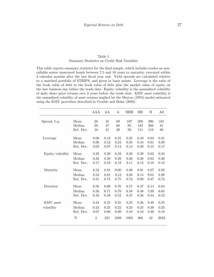
Table 1 shows summary statistics for spreads and other fundamental variables for our NAIC sample.

The variation of all the variables with rating conforms to expectations, with spread, equity volatility,

and leverage increasing on average as the rating deteriorates. There is, however, significant variation of

these variables within ratings classes. The table also reports maturity and duration, which are similar

across ratings classes for the subsample. Finally, it gives the asset volatility for firms in our sample

calculated using the KMV method as described in Crosbie and Bohn (2002), which we later use to

benchmark our own estimates of asset volatility. One interesting feature of this variable is that its

average value is relatively constant across ratings categories, apart from the B category.

INSERT TABLE 1 HERE

12For the majority of trades there are 4 annual STRIPS returns available. We use a linear approximation of the STRIPSyield curve to discount the corporate bond coupon payment which occurs between maturity dates on two STRIPS.

Expected Returns on Debt 10

4 Properties of the estimator

The purpose of the estimator is to measure the long-term expected default loss from bonds. We

do not have a long enough history of default losses on bonds in our sample, which begins in 1994, to

conduct a meaningful direct test. We therefore use three indirect tests to investigate the properties of

the estimator. The first test compares the estimates of expected default for ratings categories to those

based on historical data. The second examines the robustness of the estimates to model specification

and its sensitivity to input parameters. Finally, the information content of the estimator is tested by

studying its ability to predict ratings transitions.

4.1. Expected default losses for ratings categories

To test the properties of the estimator for ratings categories, we use the data for ratings from Huang

and Huang (2003). Table 2 shows in columns (1) to (3) the values of spreads, leverage and equity

expected return given by Huang and Huang for six ratings groups for bonds of ten years maturity,

which in this test are used as inputs to our procedure. As these are drawn by them from a variety

of sources and do not necessarily correspond to the same period of time, we use these data only to

evaluate general properties of the calibration procedure. We also need an estimate of equity volatility,

which Huang and Huang do not use. For this purpose we use the median volatility for each rating class

from our dataset of bond trades. This is given in column (4).13

To benchmark our procedure against ratings class data, we calculate default loss estimates based

on historical default experience. Elton et al. (2001) provide such estimates over different maturities

conditional on starting from a particular rating class. We use these as one benchmark. However, the

usefulness of these estimates for our purposes is limited. They assume that recovery is a function of

ratings class, whereas Altman and Kishore (1996) document that recovery rates are highly dependent

on industry and bond seniority, but not on initial rating after controlling for these variables. Moreover,

Elton et al. also assume that annual ratings transitions are Markovian, and use these to estimate

cumulative default probabilities for different horizons. Instead, we produce our own estimates of the

yield equivalent of expected default using Moody’s historical default frequencies reported in Keenan et

al. (1999), also used by Huang and Huang (2003). These are direct estimates of cumulative default

13Note that the medians are slightly different from those reported in Table 1, because to increase the quality of thestatistics here we select all trades rather than only those executed within three months after fiscal year end.

Expected Returns on Debt 11

probabilities over different time horizons, conditional on starting from a particular rating. We assume a

recovery rate for senior unsecured bonds of all ratings equal to 48.2% reported by Altman and Kishore

(1996). This recovery rate is similar to the 51.3% from Moody’s used by Huang and Huang. We combine

default probabilities and recoveries to obtain an estimate of expected default loss over the life of the

bond in a way similar to that of Elton et al. Namely, the historical default spread is the excess over the

risk-free rate of the coupon with which the bond would trade at par in a risk-neutral world, assuming

that cumulative default probabilities for each year until maturity are equal to the historical frequencies,

and that upon default the recovery rate is equal to the historical average. This coupon, C, is defined

implicitly by the relationship:

∑ (P ct − P c

t−1)R + (1− P ct )C

(1 + r)t+

1− P cT

(1 + r)T= 1

where R is the recovery rate and P ct is the cumulative probability of defaulting over t years. The spread

due to expected default risk is C − r. Our estimates of the absolute and relative historical default loss

spreads are reported in columns (10)–(11) of Table 2, and the estimates of default losses estimated by

Elton et al. for AA-BBB rated bonds are reported for comparison in column (12).

Columns (5)–(9) of Table 2 present estimation results. For each rating, we calibrate the model when

the unadjusted observed spread is used as an input, and also (except AAA) when the spread is adjusted

for non-default factors by subtracting the average AAA spread of 63 basis points. The calibrated

model parameters T, σ, and π are given in columns (5) to (7). For AAA-adjusted estimates, the asset

risk premium π is generally about 4.5% and constant across ratings groups. This suggests that our

procedure is not generating any systematic bias in the relationship between equity and asset risk. The

calibrated values of asset volatility, σ, also appear reasonable. Although they should not necessarily be

equal across ratings classes, they are sufficiently similar to suggest that most of the variation in equity

volatility reported in Table 1 is coming from differences in leverage between ratings classes rather than

differences in the nature of the assets.

The implied maturity parameter T is given in column (5). This reflects not only the actual ten

year maturity of the debt, but also any other factors ignored in the Merton model but reflected in the

spread s. The implied values of T are typically higher than the true debt maturity, which is consistent

with the fact that the under-prediction of spreads by the Merton model is less pronounced for longer

Expected Returns on Debt 12

maturities.

INSERT TABLE 2 HERE

The estimated values of the default loss spread are given in column (8) of Table 2, and column (9)

expresses them as a proportion of the full observed spread. Interestingly, in absolute terms the estimated

spread due to default is not highly sensitive to the deduction of the AAA spread. However, we believe

that the reasons for making this adjustment are so compelling that we use it throughout the rest of the

paper.

The estimated spreads due to default for AAA (unadjusted), AA, A, BBB, BB and B ratings

categories are 5, 4, 9, 21, 78, and 237 basis points out of total spreads of 63, 91, 123, 194, 320, and

470 b.p., respectively. The corresponding estimates based on historical data, reported in column (11),

are 4, 5, 8, 24, 132, and 353 b.p. For investment grade bonds, our loss estimates are consistent with

those obtained from historical default and recovery data. These ratings categories are where the Merton

model performs most poorly in tests of its absolute pricing estimates. Thus, the results suggest that

its performance in the current application is much better. For the junk grades, our estimates are lower

than those based on historical data. However, uncertainties about the estimates based on historical

data are quite large, so the correspondence between the fitted and historical default risk components

appears reasonable. Indeed, it is unlikely that the B spread of 470 basis points can be consistent with

the expected default spread of 353 basis points computed on the basis of historical data. The historical

estimate would leave only 117 basis points for liquidity, tax, bond-specific risk premia and the default

risk premium. This is significantly lower than the corresponding 188 basis points for the BBB spread,

which is difficult to justify. In contrast, our calibration-based estimates are 242 bp for BB and 233 bp

for B. Thus, our estimates appear more reasonable when they differ from those based on historical data.

Our estimates of the proportion of the spread due to expected default reported in column (8) share

one important property with the historical estimates in column (10): the proportion is increasing as

the debt quality deteriorates. This demonstrates that using either a constant value for the default risk

spread within a ratings category or even a constant proportion of the spread is unlikely to be correct,

and a procedure such as ours is necessary to estimate the default spread accurately, even within a rating

category.

As well as the spread due to default risk, which reflects the probability of default and the recovery

rate, we estimated the model-implied probabilities of default, and found that these differed markedly

Expected Returns on Debt 13

from the historical default frequencies. Even though our procedure matches the expected spread due

to default well, it gives a generally higher probability of default than the historical data. This is not

surprising given the fact that continuous models of the Merton type tend to have a high probability of

small losses in default; it is difficult to have a high loss rate in conjunction with a low probability of

default in such models.

4.2. Robustness

We study the sensitivity of the model to the values of input parameters, and also test its robustness

with respect to the precise model specification by introducing bankruptcy costs and strategic default

into the basic Merton setup. Finally, we examine whether cash distributions in the form of dividends

can change the model’s predictions significantly.

4.2.1. Sensitivity to parameters

Table 3 presents sensitivity analysis for our procedure. We use AA and BB ratings categories and

vary input parameter values. These are given in columns (1) to (5). The parameters are each varied

individually up or down by 10 percent of their base value. The results are presented in columns (6) to

(10).

INSERT TABLE 3 HERE

For both ratings categories, the estimated values of asset volatility and asset risk premia are quite robust

with respect to variation in the inputs and the structure of the model. Even when equity volatility is

varied, the asset volatility estimates remain stable. The expected default spread, δ, is also not very

sensitive to individual parameter values. Table 2 demonstrated that it is not very sensitive to the

subtraction of the AAA spread. Equation (7) shows that it does not depend at all on the risk-free

interest rate. Table 3 also shows that it is insensitive to leverage. Thus, the relatively crude measure of

leverage that we use is unlikely to be an issue. On the other hand, δ is somewhat sensitive to the estimate

of the equity risk premium. We use this sensitivity below when we invert the procedure to estimate

equity premia when expected default loss δ is given. The one variable to which the expected default

spread shows high elasticity is equity volatility, σE . Second moments such as σE can be estimated quite

accurately for equity returns. Thus, the procedure has the merit of giving a result that is sensitive only

Expected Returns on Debt 14

to a parameter that can be observed relatively accurately.

4.2.2. Sensitivity to model specification

To test robustness to model specification, we also use a simple variation of the Merton model which

allows for liquidation costs and strategic debt service of the Anderson and Sundaresan (1996) type, as

suggested by Davydenko and Strebulaev (2003). The model is described in the Appendix. It requires

another parameter θ, which can be thought of as the proportional deadweight loss in bankruptcy. When

bankruptcy costs and strategic debt service are introduced into the model, the implied value of maturity

T inversely depends on the assumed bankruptcy cost θ. In particular, we can solve for the level of θ

which makes the implied value of T equal to the actual ten year maturity of the debt.

Columns (2) and (3) of Table 4 give the results of these estimates, first using bankruptcy cost of 5%

of the debt face value suggested by Anderson and Sundaresan, and then solving for θ using the actual

10 year maturity for T . Thus adjusted, the model produces higher values of the expected loss, but the

increase is not substantial. For the BB bond it is 30 basis points of of the total spread of 320 basis

points, and it is much smaller for the AA bond. These are small proportions of the total spread. The

results therefore do not appear highly sensitive to model specification.

INSERT TABLE 4 HERE

The values of bankruptcy costs which make the Merton model consistent with the AAA-adjusted ob-

served spread are 36% of the face value for the AA bond, and 12% for the BB bond. The latter is within

the 10-20% range for bankruptcy costs estimated by Andrade and Kaplan (1998), which is consistent

with the fact that the Merton model predicts spreads for low-grade bonds reasonably well. The former

is higher than bankruptcy costs estimates of Adrade and Kaplan. However, for the AA bond the es-

timated expected loss δ is invariably very small regardless of the assumptions of the model. For both

bonds, the estimate of δ is not highly sensitive to our choice of the calibration method for the Merton

model, in which T is a free parameter.

Expected Returns on Debt 15

4.2.3. Sensitivity to dividends

The version of the Merton model that we use does not include distributions in the form of dividends

or coupons on debt. We deal with the debt structure by allowing the maturity of debt to be endogenous.

To test for sensitivity to dividends, we amend the standard Merton model by assuming that the firm

pays continuous dividends that are a constant proportion γ of the value of the firm V , as described in

the Appendix.

Columns (4)–(6) of Table 4 report the results of model calibration for different values of the instan-

taneous equity dividend yield g = γ/(1 − w). For the AA bond, the expected default loss estimate

changes by less than 1 basis point when the dividend yield rises from zero to 2% of the equity value.

For the BB debt, the corresponding change in δ is less than 19 basis points, which is almost a quarter

of the base case prediction, but still less than 6 per cent of the total observed spread. Thus, substantial

variation in the dividend yield has little impact on the proportion of the spread that is due to expected

default. The dividend yield does, however, have a major impact on the implied maturity of the debt,

T . It brings this down from the high values shown in Table 2 to levels considerably closer to the actual

ten years of maturity.

4.2.4. Summary of robustness

We find that the estimate of the expected default loss generated by our procedure is not very sensitive

to the values of the input parameters other than equity volatility. Although different model specifications

or assumptions about cash distributions result in a wide range of values for calibrated model parameters,

the resulting default loss estimate does not vary nearly as much. Across all specifications and input

values reported, for AA bonds the expected default spread δ is invariably less than 7 per cent of the

total observed spread. Thus, it is safe to conclude that the expected default spread is a very small

proportion of the observed high-quality bond spread. For BB debt, the expected default component of

the spread is between 16 and 32 percent of the total spread. Although this is a substantial variation, it

reflects a very wide range of parameter values and model structures. We conclude that the split of the

spread between expected default and other components is robust to model specification and the choice

of the parameter values.

Expected Returns on Debt 16

4.3. Expected default losses for individual bonds

Table 5 shows the estimates of the expected default loss for individual bonds in our sample. The

calibration produces well-behaved estimates of asset volatility and risk premia. In particular, like the

KMV estimates shown in Table 1, the asset volatility estimates are similar across ratings classes. The

main difference is that they do not exhibit the high estimate for the B class that is produced by the

KMV procedure.

INSERT TABLE 5 HERE

The estimates of δ are on average consistent with those based on ratings class data examined earlier.

However, there is large variation within ratings classes. The coefficients of variation are greater than one

for all but the B class, for which the cross-sectional standard deviation is large in absolute magnitude

(124 b.p.) but lower than the mean spread (196 b.p.). These results indicate that using estimates of

expected default averaged across a ratings group may be misleading if applied to individual bonds in

the group. In particular, because of the large variation within each ratings category, methods which

largely rely on ratings to estimate the expected default for individual bonds may be inaccurate.

One could argue that, although there is variation in values of δ within ratings classes, they may

be accompanied by roughly proportional changes in the spread s, and therefore one could assume a

constant default loss proportion δ/s for ratings classes. Table 5 demonstrates that, although this ratio

is indeed slightly less variable within ratings categories than the absolute value of δ, it still exhibits

significant variation. Therefore, the use of our estimation procedure appears preferable if estimates of

losses for individual bonds are required.

4.4. Prediction of ratings transitions

The most direct test of the empirical validity of our estimator of the expected loss would be to

compare actual realized losses with those estimated ex ante using the model. However, our data for

individual bonds are for the period 1994–1999, whereas the predicted loss is for the actual bond maturity

period of 7.5-10 years. We therefore cannot apply the direct test. Instead we test the information content

of δ by relating it to future rating transitions for individual bonds. Since rating transitions precede

Expected Returns on Debt 17

default, any variable that predicts ratings transitions is likely to contain information about expected

default. We regress three-year rating transitions in notches on the beginning of the period expected

default loss estimate δ.14 For homogeneity, we use only BBB bonds, because higher grade bonds have

much lower expected losses, and lower grade bonds are much less frequent. We compare the predictive

ability of δ with regards to the rating transition over the next three years with a linear regression on

the three input variables: spread, leverage and volatility. Table 6 presents the result of this test.

INSERT TABLE 6 HERE

In specification (1), for each year’s subsample of trades we estimate the following equation:

(rating change)i = const + β1si + β2w

i + β3σiE + εi

This regression appears to suffer from overfitting in the sense that the coefficient estimates change a

lot from year to year, and the variables with the highest predictive poser also varies. In regression (2)

we use a linear combination of the variables, using the weights from the prior year’s regression. These

are the weights that could be used in practice to estimate expected default, because they are known ex

ante. The final regression (3) uses only the expected loss δ as the independent variable.

For each year other than 1994 the raw variables have significant predictive power for three-year

ratings transitions (see specification (1)). The expected default variable, δ, is also significant in all

years other than 1996 (specification (3)), although the R2 in these univariate regressions is lower in all

years except 1994. This suggests that the individual input variables together contain more information

than the derived scalar loss predictor δ. However, year-by-year regression coefficients for the three input

variables are highly unstable. The ex ante choice of weights for these variables for the linear combination

which best predicts rating transitions for the future is therefore problematic. In practice, one could use

the previous year’s coefficients together with the current year’s observations of the inputs to form an ex

ante predictor. Specification (2) reports the results of regressing actual three-year transitions on this

predictor.15 The results for this variable are much worse than for the expected default variable in all

years other than 1999. In most years it contains very little information. Thus, although ex post the

spread, leverage and volatility appear to be informative with regards to ratings transitions, it is difficult

14We use a regression rather than an ordinal procedure, such as probit or logit, because ratings notches are proxies forthe cardinal variable expected loss, rather than just categories.

15This variable still contains some ex post information, as the coefficients on which it is based come from three-yearratings transitions.

Expected Returns on Debt 18

to decide what combination of them should be used to form the prediction. By contrast, the estimated

default loss δ is a theory-based non-linear function of the three inputs, which is known ex ante. In

summary, the expected default variable is a significant predictor of ratings transitions and performs at

least as well as a linear combination of its constituent variables that can be specified ex ante.

5 Equity risk premia estimates

Our approach can also be used to estimate equity risk premia from debt yields if expected bond

losses are known from an independent source. The equity risk premium is one of the most important

parameters in corporate finance and valuation, and its value is the subject of great controversy (Welch,

2000). Even small differences in estimates can have a major effect on valuations, and estimates ranging

from 0% to more than 12% have been advocated. The reason for the disagreement is that all estimates

are potentially subject to large standard errors. The equity risk premium is such an important and

controversial parameter that any extra information that assists in its estimation is potentially very

valuable. The advantage of using our approach for this purpose is that it relies on debt spreads and

other observable capital market variables which aggregate agents’ expectations about future returns. It

avoids the measurement problems of other expectational variables, such as the analysts’ forecasts used

by Harris and Marston (1992).

To estimate equity risk premia, we equate the expected loss computed using our procedure to

historical bond default losses by varying the equity risk premium used as an input, as follows. First, for

each bond in the sample, we use cumulative default probabilities documented in Keenan et al. (1999)

in conjunction with the historical average recovery rate on senior unsecured bonds of 48.2% reported

in Altman and Kishore (1996), to calculate the historical default loss δh for the maturity of the bond.

Second, we find asset and equity premia, π and πE , which make equations (7) and (6) hold when δ=δh.

Table 7 presents our results.

Across our sample of firms, the mean equity premium is 4.8%, and the asset premium 3.3%. These

estimates are lower than those usually obtained from unadjusted historical averages. For instance,

Brealey and Myers (2003) report an average premium for equities relative to treasury bills of 9.1% based

on the period 1926–2000. Our estimates are closer to those of Dimson et al. (2001), who use a different

historical period and make various adjustments to the raw historical averages. For ratings classes, the

equity premia estimates range from 3.1% for AA companies to 8.5% for B companies, reflecting the

Expected Returns on Debt 19

different leverage in the different ratings classes. The asset risk premia exhibit less variability and no

clear pattern across ratings.

INSERT TABLE 7 HERE

Apart from the robustness of our calibration approach, the validity of these estimates depends on the

usability of the historical default data for ratings groups as predictions of future default probabilities for

individual bonds in the sample. As the procedure is applied to individual bonds, the heterogeneity of

expected default probability within rating groups and in time is likely to be an issue. Nevertheless, we

believe that the reported equity premia estimates are at least suggestive, and can be used as cross-checks

for other estimates reported in the literature.

6 Applications and extensions

6.1. Applications

The expected return on debt plays a central role in many applications. Here we discuss three: in

lending, portfolio management, and corporate finance.

The expected default loss is an important input to lending decisions and assessment of lending risk

and performance. The expected return on a debt portfolio is the promised return net of the expected

loss. Existing default loss estimation methods which do not use market yields may produce signals

inconsistent with current yields. For instance, if expected loss is based on the ratings class, the highest

yield bonds in the class will appear to have the highest expected return, even if the high yield is really

due to higher expected loss. Our procedure, on the other hand, is calibrated to market yield spreads,

and will not produce speculative forecasts of default. It can therefore be used as a benchmark against

which to judge other default forecasts and risk models, as it allows to estimate what part of a credit

forecast is based on beliefs that are speculative relative to the those implicit in current market prices.

A similar issue of using market consensus beliefs as a neutral expectation arises in portfolio man-

agement. In deciding how much risky debt to hold in a portfolio, the expected return plays a key role.

Our method enables one to extract the market consensus expected return, which should assist in deter-

mining the neutral holding of each bond. Holdings based on speculative views will involve deviations

from this neutral holding, and should be based on the difference between the speculative view and the

Expected Returns on Debt 20

market consensus view.

An important corporate finance application of the method is accounting for expected default in

calculations of the cost of debt for use in the cost of capital. Standard methods of cost of debt estimation

assume that the cost of debt is equal to either the promised yield on newly-issued debt of the firm or

the risk-free rate. Both approaches fail to make a proper adjustment for the possibility of default.

Neither is correct when only a part of the yield spread is due to expected default. The errors are most

significant when the debt is risky. As Brealey and Myers (2003) say: ‘This is the bad news: There is no

easy or tractable way of estimating the rate of return on most junk debt issues’ (p. 530). Our method

helps to overcome this problem.

6.2. Extensions

The method proposed in this paper can be varied, extended and applied in many ways. For instance,

we calibrate to the yield spread assuming that leverage is observable but debt maturity in the model is

not. We could, alternatively, calibrate to the yield spread using the procedure of Delianedis and Geske

(2001), which assumes that the market value of debt is unobservable and generates an implied firm value.

Another extension would be to use different structural models to split the observed spread. Although we

have performed a number of robustness tests, alternative specifications and models could be examined.

In particular, the modelling of volatility, which is by far the most influential input to our procedure,

may be extended. Also, spread adjustment for non-default factors may warrant research effort; in

particular, a more complex model of liquidity could be used to address cross-sectional variation in this

component. Finally, the rapidly emerging market for credit swaps is likely to provide an alternative

source of information on default risk expectations.16

7 Summary

This paper derives and tests a method of extracting the expected default loss on a corporate bond

from its yield spread. The estimate also incorporates information from leverage, equity volatility and

equity risk premia. The spread is adjusted for factors other than default risk by subtracting the AAA

spread. The remainder is then split into expected default loss and risk premium using the Merton

16Longstaff et al. (2003) provide evidence on relative pricing of corporate bonds and credit default swaps.

Expected Returns on Debt 21

(1974) model of risky debt pricing. The idea of the method is to extract current forward-looking

market expectations about future default losses incorporated in observed debt and equity prices. The

method does not rely on historical data, can be applied to individual bonds, and does not produce

signals that would be speculative relative to current market yields.

We test robustness of the method by varying the structure of the model used to split the spread,

and its parametrization. The procedure, though based on the simplest contingent-claims model of risky

debt, is found to be robust in estimating the default loss component of the spread. We believe that

this robustness comes from the fact that all models of risky debt must preserve the basic structure

of debt and equity: that debt is senior to equity. This makes the choice of the particular structural

model secondary when the goal is splitting the observed market spread into default and non-default

components. We find that predicted default losses are consistent with historic experience for different

rating classes. We test the ability of the estimator to predict ratings transitions and show that it appears

to incorporate much of the information contained in spreads, leverage and volatility. It predicts three-

year rating transitions with an R2 of about 10 percent. However, an important aspect of the estimator

is that it is sensitive to the forecast of volatility; this is an aspect of the estimation procedure that could

be extended to possibly improve the estimator.

The method has many possible applications in lending decisions, bank regulation, portfolio building,

risk management, performance evaluation and cost of capital analysis. We use it to provide an entirely

new set of equity risk premium estimates, based on data hitherto unused for this purpose. We obtain

asset risk premia estimates of about three percent, while equity risk premia vary from three to nine

percent depending on the firm’s rating.

Appendix

In its standard form, the Merton model states that:

B = V N(−d1)− Fe−rT N(d2) (A.1)

where V is the value of the assets of the firm, B is the value of the debt, F is the promised debt payment (theface value of the debt for a zero-coupon bond), and:

d1 = [ln[V/F ] + (r + σ2/2)T ]/σ√

T (A.2)

d2 = d1 − σ√

T (A.3)

Expected Returns on Debt 22

The promised debt yield spread over Treasury, and the financial leverage are given by:

s =1

Tln

F

B− r (A.4)

w = B/V (A.5)

Substitution of (A.4)-(A.5) into (A.1)-(A.3) yields equations (2)-(4) in the main text.

From the dynamics of the firm’s assets given by (1) it follows that the value of assets at debt maturity VT

is:

VT = V e(r+π−σ22 )T+σ

√TZ (A.6)

where Z is a standard normal variable, and the asset risk premium π = µ− r. Then, the yield spread which isdue to the expected default loss over the maturity period is found from:

BeδT =

∫Z: VT <F

(F − VT ) dN(Z) (A.7)

Evaluating the integral yields equation (7) of the main text.

The basic Merton model can be perturbed to account for bankruptcy costs and strategic default similarto that of Anderson-Sundaresan (1996), as suggested in Davydenko and Strebulaev (2003). In this model thetransfer of the firm’s assets to bondholders in bankruptcy involves a fixed cost of H. Moreover, the debtcontract can be renegotiated, and bankruptcy does not automatically occur when equityholders fail to repayF to bondholders at maturity. In equilibrium, equityholders make opportunistic take-it-or-leave-it offers tobondholders regarding the level of debt repayment, which may be lower than the contracted amount F but highenough to persuade bondholders to renegotiate the debt rather than demand costly bankruptcy. The equilibriumpayoff to debt at maturity is:

BT = min{F, max{VT −H, 0}}The value of the bond is:

B = Call(H)− Call(F + H) =

= V[N(dH

1 )−N(dF+H1 )

]+ Fe−rT

[(1 + θ)N(dF+H

2 )− θN(dH2 )

]where θ = H/F is the bankruptcy cost expressed as a fraction of the debt par value, and:

dH1 =

[− ln w − (s− σ2/2)T

]/σ√

T − ln θ/σ√

T

dF+H1 =

[− ln w − (s− σ2/2)T

]/σ√

T − ln(1 + θ)/σ√

T

di2 = di

1 − σ√

T , i = H, F + H

Dividing by B yields:

1 =[N(dH

1 )−N(dF+H1 )

]/w + esT

[(1 + θ)N(dF+H

2 )− θN(dH2 )

](A.8)

Ito’s lemma also implies that:

σE/σ =∂E

∂VV/E =

[1−N(dH

1 ) + N(dF+H1 )

]/(1− w) (A.9)

The system of equations (A.8)-(A.9) is analogous to system (2)-(5) in the basic specification of the model.For a given value of θ we can solve the system to determine T and σ which are consistent with the observedfirm’s characteristics w, σE , and s. Alternatively, assuming that T is known, θ can be treated as an unknownparameter which makes the model consistent with the observed spread. In this case, the system can be solvedfor θ and σ instead. Once this is done, the expected loss over the maturity period is:

δ = − 1

Tln

[e(π−s)T N(KH

1 )−N(KF+H1 )

w+ (1 + θ)N(KF+H

2 )− θN(KH2 )

](A.10)

Expected Returns on Debt 23

Kij = di

j − π√

T/σ, i = H, F + H, j = 1, 2

which is the analog of formula (7) for this case.

Another robustness check of the model we perform is a test of its sensitivity to cash distributions. To thisend, we assume in the basic model that the firm pays continuous dividends that are a constant proportion γ ofthe value of the firm V . The instantaneous equity dividend yield is then g = γ/(1− w).

Repeating the analysis under this assumption, equations (2)–(7) become:

e−γT N(−d1)/w + esT N(d2) = 1 (A.11)

where

d1 = [− ln w − (s + γ − σ2/2)T ]/σ√

T (A.12)

d2 = d1 − σ√

T (A.13)

and:(1− w)σE = σ[1− e−γT N(−d1)] (A.14)

δ = − 1

Tln

[e(π−γ−s)T N

(−d1 − (π − γ)

√T/σ

)/w + N

(d2 + (π − γ)

√T/σ

)](A.15)

Expected Returns on Debt 24

References

[1] Acharya, V.V., Bharath, S.T., and Srinivasan, A., 2003. Understanding the Recovery Rates on

Defaulted Securities. Working paper. London Business School.

[2] Altman E.I., 1968. Financial ratios, discriminant analysis and the prediction of corporate

bankruptcy. Journal of Finance 23, 589-609.

[3] Altman, E.I., and Kishore, V.M., 1996. Almost Everything You Wanted To Know About Recoveries

on Defaulted Bonds. Financial Analysts Journal, November/December, 57-64.

[4] Altman E.I., and Rijken, H.A., 2003. Benchmarking the Timeliness of Credit Agency Ratings with

Credit Score Models. Working paper. NYU Salomon Centre.

[5] Anderson R.W., and Sundaresan, S., 1996. The Design and Valuation of Debt Contracts. Review

of Financial Studies 9, 37-68.

[6] Andrade, G., and Kaplan, S.N., 1998. How Costly Is Financial (Not Economic) Distress? Evidence

from Highly Leveraged Transactions That Became Distressed. Journal of Finance 53, 1443-1493.

[7] Asquith, P., Mullins, D.W., and Wolff, E.D., 1989. Original Issue High Yield Bonds: Aging Analyses

of Defaults, Exchanges, and Calls. Journal of Finance 44, 923-52.

[8] Bhandari, L.C., 1988. Debt/Equity Ratio and Expected Common Stock Returns: Empirical Evi-

dence. Journal of Finance 43, 507-528.

[9] Black, F., and Cox, J.C., 1976. Valuing Corporate Securities: Some Effects of Bond Indenture

Provisions. Journal of Finance 31, 351-367.

[10] Brealey, R.A., and Myers, S.C, 2003. Principles of Corporate Finance. 7th Edition, McGraw-Hill.

[11] Collin-Dufresne P., and Goldstein, R.S., 2001. Do Credit Spreads Reflect Stationary Leverage

Ratios? Journal of Finance 56, 1929-1957.

[12] Collin-Dufresne P., Goldstein, R.S., and J.S. Martin, 2001. The Determinants of Credit Spread

Changes. Journal of Finance 56, 2177-2207.

[13] Crosbie, P.J., and Bohn, J.F., 2002. Modeling Default Risk. Working paper. KMV LLC.

[14] Crouhy, M., Galai, D., and Mark, R., 2000. A Comparative Analysis of Current Credit Risk Models.

Journal of Banking and Finance 24, 59-117.

Expected Returns on Debt 25

[15] Davydenko, S. A., and Strebulaev, I.A., 2003. Strategic Actions and Credit Spreads: An Empirical

Investigation. Mimeo. London Business School.

[16] Delianedis, G. and Geske, R., 2001, The Components of Corporate Credit Spreads: Default, Re-

covery, Tax, Jumps, Liquidity, and Market factors. Working paper 22-01. Anderson School, UCLA.

[17] Dimson, E., Marsh, P., and Staunton, M., 2001. Millennium Book II: 101 Years of Investment

Returns. ABN Amro/London Business School.

[18] Duffie D., and K. J. Singleton, 1999. Modeling Term Structures of Defaultable Bonds. Review of

Financial Studies 12, 687-720.

[19] Elton E.J., Gruber, M.J., Agrawal, D., and Mann, C., 2001. Explaining the Rate Spread on

Corporate Bonds. Journal of Finance 56, 247-277.

[20] Eom Y.H., Helwege, J., and Huang, J., 2003. Structural Models of Corporate Bond Pricing: An

Empirical Analysis. Review of Financial Studies, forthcoming.

[21] Geske, R., 1977. The Valuation of Corporate Securities as Compound Options. Journal of Financial

and Quantitative Analysis 12, 541-552.

[22] Hand, J.R., Holthausen, R.W., and Leftwich, R.W, 1992. The Effect of Bond Rating Agency

Announcements on Bond and Stock Prices. Journal of Finance. 47, 733-752.

[23] Harris, R. and Marston, F., 1992. Estimating Shareholder Risk Premium Using Analysts’ Growth

Forecasts. Financial Management, 63-70.

[24] Huang, J., and Huang, M., 2003. How Much of the Corporate-Treasury Yield Spread is Due to

Credit Risk? Working paper, Penn State University.

[25] Jarrow R.A., Lando D., and Yu, F., 2003. Default Risk and Diversification: Theory and Applica-

tions. Working paper. Cornell University.

[26] Jones E.P., Mason, S.P., and Rosenfeld, E., 1984. Contingent Claims Analysis of Corporate Capital

Structures: An Empirical Analysis. Journal of Finance 39, 611-627.

[27] Keenan S.C., Shtogrin, I., and Soberhart, J., 1999. Historical Default Rates of Corporate Bond

Issuers, 1920-1998. Working paper. Moody’s Investor Service.

Expected Returns on Debt 26

[28] Leland H.E., 1994. Corporate Debt Value, Bond Covenants, and Optimal Capital Structure. Jour-

nal of Finance 49, 1213-1251.

[29] Leland H.E., and Toft, K.B., 1996. Optimal Capital Structure, Endogenous Bankruptcy, and the

Term Structure of Credit Spreads. Journal of Finance 51, 987-1019.

[30] Longstaff F.A., Mithal, S., and Meis, E., 2003. The Credit-Default Swap Market: Is Credit Pro-

tection Priced Correctly? Working paper. UCLA.

[31] Longstaff F.A., and Schwartz, E.S., 1995. A Simple Approach to Valuing Risky Fixed and Floating

Rate Debt. Journal of Finance 50, 789-819.

[32] Mella-Barral, P., and Perraudin, W., 1997. Strategic Debt Service. Journal of Finance 52, 531-556.

[33] Merton R.C., 1974. On the Pricing of Corporate Debt: The Risk Structure of Interest Rates.

Journal of Finance 29, 449-470.

[34] Welch I., 2000. Views of Financial Economists on the Equity Premium and on Professional Con-

troversies. Journal of Business 73, 501-537.

Expected Returns on Debt 27

Table 1Summary Statistics on Credit Risk Variables

This table reports summary statistics for the final sample, which includes trades on non-callable senior unsecured bonds between 7.5 and 10 years to maturity, executed within3 calendar months after the last fiscal year end. Yield spreads are calculated relativeto a matched portfolio of STRIPS, and given in basis points. Leverage is the ratio ofthe book value of debt to the book value of debt plus the market value of equity onthe last business day before the trade date. Equity volatility is the annualized volatilityof daily share price returns over 2 years before the trade date. KMV asset volatility isthe annualized volatility of asset returns implied by the Merton (1974) model estimatedusing the KMV procedure described in Crosbie and Bohn (2002).

AAA AA A BBB BB B All

Spread, b.p. Mean 28 45 69 107 208 396 101Median 28 47 66 95 182 369 81Std. Dev. 10 21 39 50 111 119 80

Leverage Mean 0.06 0.13 0.25 0.35 0.49 0.63 0.31Median 0.06 0.12 0.24 0.35 0.44 0.61 0.29Std. Dev. 0.03 0.07 0.14 0.14 0.20 0.15 0.17

Equity volatility Mean 0.33 0.30 0.33 0.33 0.39 0.62 0.34Median 0.33 0.28 0.29 0.30 0.38 0.62 0.30Std. Dev. 0.17 0.10 0.12 0.11 0.12 0.18 0.12

Maturity Mean 8.53 8.81 9.00 8.86 8.91 8.87 8.92Median 8.53 8.81 9.12 8.88 9.15 9.01 8.99Std. Dev. 0.21 0.75 0.75 0.74 0.69 0.87 0.74

Duration Mean 6.56 6.69 6.76 6.57 6.47 6.14 6.64Median 6.56 6.71 6.79 6.58 6.48 5.99 6.65Std. Dev. 0.16 0.48 0.52 0.47 0.56 0.54 0.52

KMV asset Mean 0.24 0.25 0.25 0.25 0.26 0.49 0.25volatility Median 0.24 0.25 0.22 0.23 0.25 0.39 0.23

Std. Dev. 0.07 0.06 0.09 0.10 0.10 0.30 0.10

N 2 231 1088 1003 266 42 2632

Expected Returns on Debt 28Tab

le2

Est

imat

edex

pect

edde

faul

tlo

sses

The

tabl

egi

ves

mod

el-p

redi

cted

expe

cted

defa

ult

loss

esan

dpr

obab

iliti

esfo

rge

neri

cbo

nds

in6

rati

nggr

oups

.T

hese

cond

colu

mn

indi

cate

sw

heth

erth

eob

serv

edsp

read

was

adju

sted

for

non-

defa

ult

fact

ors

bysu

btra

ctin

gth

eav

erag

esp

read

onA

AA

bond

s.T

hein

puts

are

mea

nva

lues

inea

chra

ting

clas

sof

the

prom

ised

spre

adon

debt

s,le

vera

gew

,an

das

sum

edeq

uity

risk

prem

ium

,π

E,as

used

inH

uang

and

Hua

ng(2

003)

;an

dth

em

edia

nvo

lati

lity

ofeq

uity

σE

from

our

stud

ied

sam

ple.

T,

σan

dπ

are

mod

el-im

plie

dm

atur

ity,

vola

tilit

yof

asse

tsan

das

set

risk

prem

ium

.T

heou

tput

sis

the

pred

icte

dex

pect

edde

faul

tlo

sson

debt

δ.δ h

isth

eex

cess

over

the

risk

-fre

era

teof

the

coup

onra

teon

a10

-yea

rbo

ndw

ith

defa

ult

prob

abili

ties

inea

chye

ar1–

10eq

ualto

thos

ere

port

edby

Moo

dy’s

inK

eena

net

al.

(199

9),

and

are

cove

ryra

teof

48.2

%,

whi

chm

akes

its

risk

-neu

tral

valu

eeq

ualto

par.

δ EG

isth

ede

faul

tlo

ssfo

ra

10-y

ear

bond

esti

mat

edin

Elt

onet

al.

(200

1).

Mod

elM

odel

Def

ault

loss

Spre

adin

puts

para

met

ers

Mod

elH

isto

rica

lE

GR

atin

gad

just

-s

wπ

Eσ

ET

σπ

δδ/

sδ h

δ h/s

δ EG

men

tb.

p.%

yrs.

%b.

p.b.

p.b.

p.(1

)(2

)(3

)(4

)(5

)(6

)(7

)(8

)(9

)(1

0)(1

1)(1

2)

AA

AN

one

630.

135.

380.

2751

.08

0.24

4.83

5.36

0.09

3.95

0.06

AA

Non

e91

0.21

5.60

0.28

51.9

70.

234.

749.

450.

105.

410.

064.

80A

AA

2819

.60

0.22

4.51

3.87

0.04

AN

one

123

0.32

5.99

0.29

49.8

60.

234.

6815

.58

0.13

8.33

0.07

14.0

0A

AA

6022

.97

0.21

4.37

9.46

0.08

BB

BN

one

194

0.43

6.55

0.31

65.3

80.

234.

9126

.85

0.14

24.4

00.

1340

.90

AA

A13

135

.22

0.21

4.51

21.2

80.

11

BB

Non

e32

00.

547.

300.

3843

.05

0.27

5.07

93.0

20.

2913

2.24

0.41

AA

A25

729

.25

0.25

4.73

78.1

50.

24

BN

one

470

0.66

8.76

0.57

9.87

0.30

4.54

271.

340.

5835

2.87

0.75

AA

A40

78.

270.

284.

3323

6.70

0.50

Expected Returns on Debt 29

Table 3Sensitivity to Parameter Values

For the generic AA and BB bonds from Table 2, this table reports the sensitivity of thepredicted expected default loss to model inputs, obtained by decreasing and increasingthe base values of individual parameters by 10%. The inputs are the promised spreadon debt s adjusted for non-default factors by subtracting the average AAA spread (sadj. is the adjusted spread value), leverage w, equity risk premium, πE , and equityvolatility, σE . The outputs are model-implied maturity T , volatility of assets σ, assetrisk premium π, and the predicted expected default loss on debt, δ.

Model inputs Parameter estimatess s adj. w πE σE T σ π δ δ/s

b.p. b.p. % % b.p.(1) (2) (3) (4) (5) (6) (7) (8) (9) (10)

Panel A: Typical AA-rated bonds

91 28 0.21 5.60 0.28 19.60 0.22 4.51 3.87 0.04382 19 15.80 0.22 4.48 2.77 0.034100 37 23.44 0.22 4.55 4.87 0.049

0.19 20.88 0.23 4.62 3.63 0.0400.23 18.51 0.22 4.40 4.09 0.045

5.04 19.60 0.22 4.06 4.85 0.0536.16 19.60 0.22 4.96 3.06 0.034

0.25 27.61 0.20 4.54 2.09 0.0230.30 14.53 0.24 4.49 5.83 0.064

Panel B: Typical BB-rated bonds

320 257 0.54 7.30 0.38 29.25 0.25 4.73 78.15 0.244288 225 24.03 0.24 4.56 70.10 0.243352 289 35.56 0.26 4.90 85.86 0.240

0.48 30.23 0.26 5.01 75.96 0.2370.59 28.71 0.23 4.44 80.10 0.25.0

6.57 29.25 0.25 4.26 90.00 0.2818.03 29.25 0.25 5.20 67.47 0.211

0.34 52.26 0.24 5.06 51.14 0.1600.42 18.35 0.26 4.49 101.86 0.318

Expected Returns on Debt 30

Table 4Robustness To Model Specification and Dividend Yield

For the generic AA and BB bonds from Table 2, this table reports the sensitivity of thepredicted expected default loss to model assumptions and cash distributions. Column (1)reports base-case results for the standard model. Columns (2) and (3) report results ofthe modified model with proportional bankruptcy costs θ and strategic default. Columns(4) to (6) report results of a modified model that allows cash dividend distributions whichare a constant fraction of the firm’s value, for different levels of the instantaneous dividendyield as a proportion of equity value, g. The inputs are the promised spread on debt sadjusted for non-default factors by subtracting the average AAA spread (s adj. is theadjusted spread value), leverage w, equity risk premium, πE , and equity volatility σE .The outputs are model-implied maturity T , volatility of assets σ, asset risk premium π,and the predicted expected default loss on debt, δ. The details of the model modificationsare described in the Appendix.

Base case Strategic default Dividendsθ = 0 θ = 5% T = 10 g = 1% g = 2% g = 3%(1) (2) (3) (4) (5) (6)

Panel A: Typical AA-rated bonds=91 b.p., s adj. =28 b.p., w = 0.21, πE = 5.60%, σE = 0.28

T 19.6 17.6 10 16.3 14.0 12.4σ 0.22 0.22 0.22 0.22 0.22 0.22π, % 4.51 4.51 4.49 4.51 4.50 4.50θ, % – 5 36 – – –δ, b.p. 3.87 4.16 5.99 4.08 3.02 0.42δ/s, % 0.043 0.046 0.066 0.045 0.033 0.005

Panel B: Typical BB-rated bonds=320 b.p., s adj.=257 b.p., w = 0.54, πE = 7.30%, σE = 0.38

T 29.3 16.9 10 19.4 14.9 12.3σ 0.25 0.24 0.23 0.24 0.24 0.23π, % 4.73 4.60 4.45 4.60 4.51 4.45θ, % – 5 12 – – –δ, b.p. 78.2 92.7 108.3 90.4 96.7 99.8δ/s, % 0.244 0.290 0.339 0.283 0.302 0.312

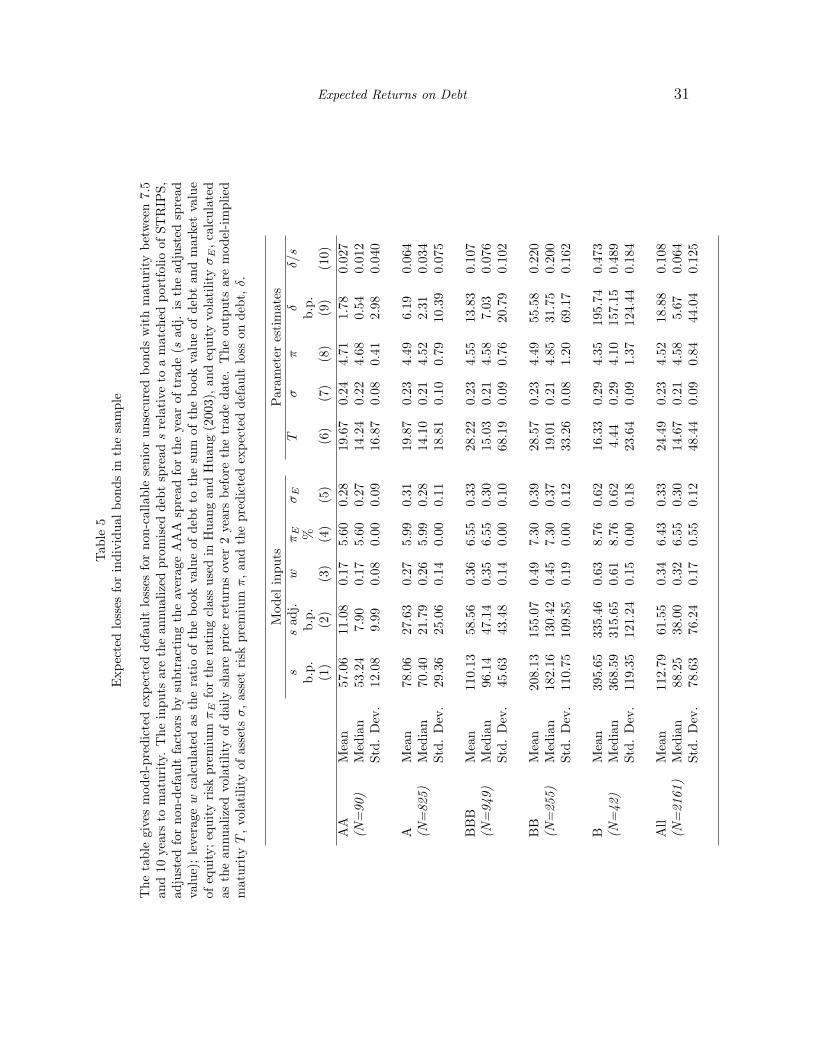
Expected Returns on Debt 31Tab

le5

Exp

ecte

dlo

sses

for

indi

vidu

albo

nds

inth

esa

mpl

e

The

tabl

egi

ves

mod

el-p

redi

cted

expe

cted

defa

ult

loss

esfo

rno

n-ca

llabl

ese

nior

unse

cure

dbo

nds

wit

hm

atur

ity

betw

een

7.5

and

10ye

ars

tom

atur

ity.

The

inpu

tsar

eth

ean

nual

ized

prom

ised

debt

spre

ads

rela

tive

toa

mat

ched

port

folio

ofST

RIP

S,ad

just

edfo

rno

n-de

faul

tfa

ctor

sby

subt

ract

ing

the

aver

age

AA

Asp

read

for

the

year

oftr

ade

(sad

j.is

the

adju

sted

spre

adva

lue)

;le

vera

gew

calc

ulat

edas

the

rati

oof

the

book

valu

eof

debt

toth

esu

mof

the

book

valu

eof

debt

and

mar

ket

valu

eof

equi

ty;e

quity

risk

prem

ium

πE

for

the

rati

ngcl

ass

used

inH

uang

and

Hua

ng(2

003)

,and

equi

tyvo

lati

lity

σE

,cal

cula

ted

asth

ean

nual

ized

vola

tilit

yof

daily

shar

epr

ice

retu

rns

over

2ye

ars

befo

reth

etr

ade

date

.T

heou

tput

sar

em

odel

-im

plie

dm

atur

ity

T,vo

lati

lity

ofas

sets

σ,as

set

risk

prem

ium

π,an

dth

epr

edic

ted

expe

cted

defa

ult

loss

onde

bt,δ.

Mod

elin

puts

Par

amet

eres

tim

ates

ss

adj.

wπ

Eσ

ET

σπ

δδ/

sb.

p.b.

p.%

b.p.

(1)

(2)

(3)

(4)

(5)

(6)

(7)

(8)

(9)

(10)

AA

Mea

n57

.06

11.0

80.

175.

600.

2819

.67

0.24

4.71

1.78

0.02

7(N

=90

)M

edia

n53

.24

7.90

0.17

5.60

0.27

14.2

40.

224.

680.

540.

012

Std.

Dev

.12

.08

9.99

0.08

0.00

0.09

16.8

70.

080.

412.

980.

040

AM

ean

78.0

627

.63

0.27

5.99

0.31

19.8

70.

234.

496.

190.

064

(N=

825)

Med

ian

70.4

021

.79

0.26

5.99

0.28

14.1

00.

214.

522.

310.

034

Std.

Dev

.29

.36

25.0

60.

140.

000.

1118

.81

0.10

0.79

10.3

90.

075

BB

BM

ean

110.

1358

.56

0.36

6.55

0.33

28.2

20.

234.

5513

.83

0.10

7(N

=94

9)M

edia

n96

.14

47.1

40.

356.

550.

3015

.03

0.21

4.58

7.03

0.07

6St

d.D

ev.

45.6

343

.48

0.14

0.00

0.10

68.1

90.

090.

7620

.79

0.10

2

BB

Mea

n20

8.13

155.

070.

497.

300.

3928

.57

0.23

4.49

55.5

80.

220

(N=

255)

Med

ian

182.

1613

0.42

0.45

7.30

0.37

19.0

10.

214.

8531

.75

0.20

0St

d.D

ev.

110.

7510

9.85

0.19

0.00

0.12

33.2

60.

081.

2069

.17

0.16

2

BM

ean

395.

6533

5.46

0.63

8.76

0.62

16.3

30.

294.

3519

5.74

0.47

3(N

=42

)M

edia

n36

8.59

315.

650.

618.

760.

624.

440.

294.

1015

7.15

0.48

9St

d.D

ev.

119.

3512

1.24

0.15

0.00

0.18

23.6

40.

091.

3712

4.44

0.18

4

All

Mea

n11

2.79

61.5

50.

346.

430.

3324

.49

0.23

4.52

18.8

80.

108

(N=

2161

)M

edia

n88

.25

38.0

00.

326.

550.

3014

.67

0.21

4.58

5.67

0.06

4St

d.D

ev.

78.6

376

.24

0.17

0.55

0.12

48.4

40.

090.

8444

.04

0.12

5

Expected Returns on Debt 32

Table 6Predicting rating transitions

The table reports the results of regression analysis of rating predictions by year of trade. The dependentvariable is the rating transition in notches in 3 years subsequent to the date of trade for each trade in thedataset, consisting of bonds with maturity between 7.5 and 10 years. Independent variables in specification (1)are the spread (s), leverage (w), and equity volatility (σE) for the trade. Regression (2) in each year between1995 and 1999 uses the regression coefficients for the variables s, w and σE estimated in regression (1) forthe previous year to form a linear combination of these variables. This linear combination is then used as aregressor. In regression specification (3) the independent variable is δ, the expected default spread estimatedfor the trade using the procedure. t-statistics are reported in parentheses.

Year const s w σE lagged δ R2

1994 (1) 0.95(1.16) -0.08 (-0.18) -1.44 (-1.42) -0.91 (-0.52) 3.8%(2) N/A N/A N/A(3) 0.27 (1.37) -0.026 (-1.85) 4.5%

1995 (1) 3.05 (6.86) -0.55 (-2.40) -2.43 (-3.49) -3.91 (-3.59) 24.0%(2) 0.56 (1.01) 0.37 (0.56) 0.2%(3) 0.63 (5.52) -0.029 (-5.44) 16.8%

1996 (1) -1.07 (-2.07) 0.01 (0.05) 1.90 (2.85) 2.33 (1.68) 5.2%(2) -0.13 (-0.27) -0.15 (-0.86) 0.4%(3) 0.17 (1.64) 0.011 (1.66) 1.5%

1997 (1) 2.18 (3.27) -1.43 (-2.90) 2.79 (2.61) -8.16 (-6.61) 35.1%(2) -1.51 (-2.56) 0.55 (1.53) 1.2%(3) 0.27 (1.93) -0.121 (-9.58) 32.9%

1998 (1) 3.45 (3.54) -1.70 (-4.23) -0.97 (-0.52) -5.96 (-3.37) 17.2%(2) -2.21 (-3.89) -0.23 (-2.22) 2.4%(3) -0.38 (-1.72) -0.035 (-5.60) 13.7%

1999 (1) 10.31 (8.71) 0.39 (0.89) -10.66 (-7.26) -18.65 (-9.06) 42.6%(2) -6.68 (-7.29) -0.31 (-6.83) 24.1%(3) 0.49 (1.35) -0.048 (-4.50) 12.1%

Expected Returns on Debt 33Tab

le7

Est

imat

edco

stof

equi

tyfo

rin

divi

dual

bond

sin

the

sam

ple

The

tabl

ere

port

sth

eco

stof

equi

tyva

lues

cons

iste

ntw

ith

hist

oric

alde

faul

tpr

obab

iliti

esan

dre

cove

ryra

tes.

The

sam

ple

cons

ists

ofse

nior

unse

cure

dbo

nds

wit

hm

atur

ity

betw

een

7.5

and

10ye

ars.

The

inpu

tsar

eth

ean

nual

ized

prom

ised

debt

spre

ads

rela

tive

toa

mat

ched

port

folio

ofST

RIP

S,ad

just

edfo

rno

n-de

faul

tfa

ctor

sby

subt

ract

ing

the

aver

age

AA

Asp

read

for

the

year

oftr

ade

(sad

j.is

the

adju

sted

spre

adva

lue)

;le

vera

gew

calc

ulat

edas

the

rati

oof

the

book

valu

eof

debt

toth

esu

mof

book

valu

eof

debt

and

mar

ket

valu

eof

equi

ty;

equi

tyvo

lati

lity

σE

,ca

lcul

ated

asth

ean

nual

ized

vola

tilit

yof

daily

shar

epr

ice

retu

rns

over

2ye

ars

befo

reth

etr

ade

date

;an

dth

eex

pect

edde

faul

tlo

ssfo

rth

ebo

ndδ,

esti

mat

edas

the

exce

ssov

erth

eri

sk-fre

era

teof

the

coup

onra

tew

hich

wou

ldm

ake

the

risk

-neu

tral

bond

valu

eeq

ualto

par,

assu

min

gde

faul

tpr

obab

iliti

esin

each

year

unti

lm

atur

ity

equa

lto

thos

ere

port

edby

Moo

dy’s

inK

eena

net

al.

(199

9),

and

are

cove

ryra

teof

48.2

%.

The

outp

uts

are

mod

el-im

plie

dm

atur

ity

T,v

olat

ility

ofas

sets

σ,a

sset

risk

prem

ium

π,a

ndth

eim

pute

dex

pect

edeq

uity

prem

ium

πE

.

Mod

elin

puts

Mod

elpa

ram

eter

sM

odel

ss

adj.

wσ

Eδ

Tσ

πes

tim

ate

b.p.

b.p.

b.p.

%π

E,%

(1)

(2)

(3)

(4)

(5)

(6)

(7)

(8)

(9)

AA

Mea

n61

.13

15.8

40.

180.

285.

4522

.80

0.24

2.51

3.06

(N=

58)

Med

ian

57.9

813

.02

0.20

0.27

5.46

15.5

40.

222.

092.

68St

d.D

ev.

11.9

69.

460.

080.

090.

0718

.51

0.08

2.28

2.95

AM

ean

82.5

832

.01

0.28

0.31

7.74

21.6

80.

233.

785.

30(N

=69

6)M

edia

n74

.14

25.3

00.

280.

287.

7815

.32

0.20

2.61

3.42

Std.

Dev

.29

.51

24.9

20.

140.

100.

4319

.64

0.09

3.88

5.51

BB

BM

ean

116.

6865

.53

0.37

0.33

23.5

231

.04

0.23

3.02

4.49

(N=

815)

Med

ian

103.

3252

.13

0.37

0.30

23.5

816

.59

0.20

2.03

2.98

Std.

Dev

.45

.83

43.0

30.

140.

100.

8073

.08

0.08

3.22

4.87

BB

Mea

n28

0.53

226.

460.

550.

4213

4.93

35.6

00.

242.

314.

30(N

=11

9)M

edia

n24

4.47

185.

090.

500.

4113

4.48

19.2

20.

231.

382.

44St

d.D

ev.

125.

3112

5.20

0.21

0.11

1.40

43.7

10.

092.

724.

31

BM

ean

534.

8647

5.14

0.61

0.73

367.

0514

.91

0.35

3.83

8.53

(N=

14)

Med

ian

496.

5043

8.34

0.60

0.82

368.

472.

350.

372.

916.

36St

d.D

ev.

96.3

090

.08

0.14

0.22

4.50

21.7

20.

083.

478.

34

All

Mea

n11

5.74

64.7

50.

340.

3327

.07

27.1

20.

233.

274.

79(N

=17

02)

Med

ian

91.4

541

.40

0.32

0.30

22.3

816

.38

0.21

2.20

3.18

Std.

Dev

.80

.15

77.6

40.

170.

1144

.05

53.7

30.

093.

485.

12