Using Valence Bond Theory to Model (Bio)Chemical...
49
September 7 th 2016 1 Fernanda Duarte Using Valence Bond Theory to Model (Bio)Chemical Reactivity Master Course for Theoretical Chemistry and Computational Modelling (TCCM) Department of Chemistry, Oxford
Transcript of Using Valence Bond Theory to Model (Bio)Chemical...

September 7th 2016
1
Fernanda Duarte
Using Valence Bond Theory to Model
(Bio)Chemical Reactivity
Master Course for Theoretical Chemistry and Computational
Modelling (TCCM)
Department of Chemistry, Oxford

• Motivation & History of VB
• Basic Concepts
• ab initio VB theory
• Multiscale VB simulations
• Empirical VB theory
General Outline of Lecture

33
Motivation
Concepts and heuristic models (Localised view )
Quantitative theory (Delocalised view)
Lewis model
Curly-Arrows
VSEPR
Hybridisation
...
Localised electron pairs Chemical bond concept
Delocalised particles indistinguishable and interacting
(no chemical bond)
C Y
H
HH
X
H = E

4
Historical Timeline
L. Pauling The Nature of the Chemical Bond
1929 19331927G.N. Lewis
1916
Heitler & London
A Chemist’s Guide to Valence Bond Theory, by Sason Shaik and Philippe C. Hiberty
As demonstrated by Heisenberg, the mixing of [wn(1)wm(2)] and [wn(2)wm(1)] ledto a new energy term that caused a splitting between the two wave functionsCA and CB. He called this term ‘‘resonance’’ using a classical analogy of twooscillators that, by virtue of possessing the same frequency, form a resonatingsituation with characteristic exchange energy.
In modern terms, the bonding in H2 can be accounted for by the wavefunction drawn in 1, in Scheme 1.1. This wave function is a superposition oftwo covalent situations in which, in the first form (a) one electron has a spin-up(a spin), while the other has spin-down (b spin), and vice versa in the secondform (b). Thus, the bonding in H2 arises due to the quantum mechanical‘‘resonance’’ interaction between the two patterns of spin arrangement that arerequired in order to form a singlet electron pair. This ‘‘resonance energy’’accounted for !75% of the total bonding of the molecule, and therebyprojected that the wave function in 1, which is referred to henceforth as theHL-wave function, can describe the chemical bonding in a satisfactory manner.This ‘‘resonance origin’’ of the bonding was a remarkable feat of the newquantum theory, since until then it was not obvious how two neutral speciescould be at all bonded.
In the winter of 1928, London extended the HL-wave function and drew thegeneral principles of the covalent bonding in terms of the resonance interactionbetween the forms that allow interchange of the spin-paired electrons betweenthe two atoms (10,12). In both treatments (9,12) the authors considered ionicstructures for homopolar bonds, but discarded their mixing as being too small.In London’s paper, there is also a consideration of ionic (so-called polar)bonding. In essence, the HL theory was a quantum mechanical version ofLewis’s electron-pair theory. Thus, even though Heitler and London did theirwork independently and perhaps unaware of the Lewis model, the HL-wavefunction still precisely described the shared-pair bond of Lewis. In fact, in hisletter to Lewis (8), and in his landmark paper (13), Pauling points out that theHL and London treatments are ‘entirely equivalent to G.N. Lewis’s successfultheory of shared electron pair . . .’’. Thus, although the final formulation of the
A BH H H H
A BA BOO •••
•••
B O2 Aa b
HL- Wave function Covalent-ionic superpositionin a bond, A–B
Pauling's three-electronbond
1 3
4
σg
σu
2
Scheme 1.1
ROOTS OF VB THEORY 3
Slater Determinant
1931
Rumer’s canonical structures
antiaromaticity, and its articulation by organic chemists in the 1950s!1970swill constitute a major cause for the acceptance of MO theory and the rejectionof VB theory (4).
The description of benzene in terms of a superposition (resonance) of twoKekule structures appeared for the first time in the work of Slater, as a casebelonging to a class of species in which each atom possesses more neighborsthan electrons it can share, much like in metals (21). Two years later, Paulingand Wheland (37) applied HLVB theory to benzene. They developed a lesscumbersome computational approach, compared with Huckel’s previousHLVB treatment, using the five canonical structures in 6, and approximatedthe matrix elements between the structures by retaining only close neighborresonance interactions. Their approach allowed them to extend the treatmentto naphthalene and to a great variety of other species. Thus, in the HLVBapproach, benzene is described as a ‘‘resonance hybrid’’ of the two Kekulestructures and the three Dewar structures; the latter had already appearedbefore in Ingold’s idea of mesomerism, which itself is rooted in Lewis’s conceptof electronic tautomerism (6). In his book, published for the first time in 1944,Wheland explains the resonance hybrid with the biological analogy ofmule= donkey+ horse (38). The pictorial representation of the wavefunction, the link to Kekule’s oscillation hypothesis, and to Ingold’smesomerism, which were known to chemists, made the HLVB representationvery popular among practicing chemists.
With these two seemingly different treatments of benzene, the chemicalcommunity was faced with two alternative descriptions of one of its molecularicons, and this began the VB!MO rivalry that seems to accompany chemistryto the Twenty-first Century (5). This rivalry involved most of the prominentchemists of various periods (e.g., Mulliken, Huckel, J. Mayer, Robinson,Lapworth, Ingold, Sidgwick, Lucas, Bartlett, Dewar, Longuet-Higgins,Coulson, Roberts, Winstein, Brown). A detailed and interesting account ofthe nature of this rivalry and the major players can be found in the treatment ofBrush (3,4). Interestingly, back in the 1930s, Slater (22) and van Vleck and
D1 D3
K2K1
D2
5 6
Huckel's delocalized π-MO picture
Ψ = c1(K1 + K2) + c2(D1 + D2 + D3)
c1 > c2
Pauling-Wheland's resonating picture
Scheme 1.2
6 A BRIEF STORY OF VALENCE BOND THEORY
1950
Pauling (1939)Wheland (1955)VB Textbooks
The Atom and The Molecule
Interaction Between Neutral Atoms and Homopolar Binding
Valence bond theory in Pauling’s view is a quantum chemical version of Lewis’s theory of valence
5
Historical Timeline
L. Pauling The Nature of the Chemical Bond
1929 19331927G.N. Lewis
1916
Heitler & London
A Chemist’s Guide to Valence Bond Theory, by Sason Shaik and Philippe C. Hiberty
As demonstrated by Heisenberg, the mixing of [wn(1)wm(2)] and [wn(2)wm(1)] ledto a new energy term that caused a splitting between the two wave functionsCA and CB. He called this term ‘‘resonance’’ using a classical analogy of twooscillators that, by virtue of possessing the same frequency, form a resonatingsituation with characteristic exchange energy.
In modern terms, the bonding in H2 can be accounted for by the wavefunction drawn in 1, in Scheme 1.1. This wave function is a superposition oftwo covalent situations in which, in the first form (a) one electron has a spin-up(a spin), while the other has spin-down (b spin), and vice versa in the secondform (b). Thus, the bonding in H2 arises due to the quantum mechanical‘‘resonance’’ interaction between the two patterns of spin arrangement that arerequired in order to form a singlet electron pair. This ‘‘resonance energy’’accounted for !75% of the total bonding of the molecule, and therebyprojected that the wave function in 1, which is referred to henceforth as theHL-wave function, can describe the chemical bonding in a satisfactory manner.This ‘‘resonance origin’’ of the bonding was a remarkable feat of the newquantum theory, since until then it was not obvious how two neutral speciescould be at all bonded.
In the winter of 1928, London extended the HL-wave function and drew thegeneral principles of the covalent bonding in terms of the resonance interactionbetween the forms that allow interchange of the spin-paired electrons betweenthe two atoms (10,12). In both treatments (9,12) the authors considered ionicstructures for homopolar bonds, but discarded their mixing as being too small.In London’s paper, there is also a consideration of ionic (so-called polar)bonding. In essence, the HL theory was a quantum mechanical version ofLewis’s electron-pair theory. Thus, even though Heitler and London did theirwork independently and perhaps unaware of the Lewis model, the HL-wavefunction still precisely described the shared-pair bond of Lewis. In fact, in hisletter to Lewis (8), and in his landmark paper (13), Pauling points out that theHL and London treatments are ‘entirely equivalent to G.N. Lewis’s successfultheory of shared electron pair . . .’’. Thus, although the final formulation of the
A BH H H H
A BA BOO •••
•••
B O2 Aa b
HL- Wave function Covalent-ionic superpositionin a bond, A–B
Pauling's three-electronbond
1 3
4
σg
σu
2
Scheme 1.1
ROOTS OF VB THEORY 3
Slater Determinant
1931
Rumer’s canonical structures
MO Theory Mulliken & Hund
Lennard-Jones O2
Huckel ModelBenzene
antiaromaticity, and its articulation by organic chemists in the 1950s!1970swill constitute a major cause for the acceptance of MO theory and the rejectionof VB theory (4).
The description of benzene in terms of a superposition (resonance) of twoKekule structures appeared for the first time in the work of Slater, as a casebelonging to a class of species in which each atom possesses more neighborsthan electrons it can share, much like in metals (21). Two years later, Paulingand Wheland (37) applied HLVB theory to benzene. They developed a lesscumbersome computational approach, compared with Huckel’s previousHLVB treatment, using the five canonical structures in 6, and approximatedthe matrix elements between the structures by retaining only close neighborresonance interactions. Their approach allowed them to extend the treatmentto naphthalene and to a great variety of other species. Thus, in the HLVBapproach, benzene is described as a ‘‘resonance hybrid’’ of the two Kekulestructures and the three Dewar structures; the latter had already appearedbefore in Ingold’s idea of mesomerism, which itself is rooted in Lewis’s conceptof electronic tautomerism (6). In his book, published for the first time in 1944,Wheland explains the resonance hybrid with the biological analogy ofmule= donkey+ horse (38). The pictorial representation of the wavefunction, the link to Kekule’s oscillation hypothesis, and to Ingold’smesomerism, which were known to chemists, made the HLVB representationvery popular among practicing chemists.
With these two seemingly different treatments of benzene, the chemicalcommunity was faced with two alternative descriptions of one of its molecularicons, and this began the VB!MO rivalry that seems to accompany chemistryto the Twenty-first Century (5). This rivalry involved most of the prominentchemists of various periods (e.g., Mulliken, Huckel, J. Mayer, Robinson,Lapworth, Ingold, Sidgwick, Lucas, Bartlett, Dewar, Longuet-Higgins,Coulson, Roberts, Winstein, Brown). A detailed and interesting account ofthe nature of this rivalry and the major players can be found in the treatment ofBrush (3,4). Interestingly, back in the 1930s, Slater (22) and van Vleck and
D1 D3
K2K1
D2
5 6
Huckel's delocalized π-MO picture
Ψ = c1(K1 + K2) + c2(D1 + D2 + D3)
c1 > c2
Pauling-Wheland's resonating picture
Scheme 1.2
6 A BRIEF STORY OF VALENCE BOND THEORY
1950
Pauling (1939)Wheland (1955)VB Textbooks

6
Historical Timeline
1952 1960 20001950
J. A. Pople A. Warshel
1970
A Chemist’s Guide to Valence Bond Theory, by Sason Shaik and Philippe C. Hiberty
Exp. verification Huckel rules
Valence
Dewar & Coulson Localized<—> delocalized
O2 failure
Mulliken, Nobel Prize
3rd Ed. Pauling Book
Fukui Frontier MO Theory
Woodward & Hoffmann
1965GAUSSIAN70
1980EVB
Goddard GVB
XIAMEN-99
Shaik Hiberty Landis Zhang Thrular Vogh

7
Valence Bond Theory
each is a VB structure �i
• Overall description is a linear combination of various VB structures formed by different distributions, arrangements and/or pairing of these electrons.
• VB theory describes system as a collection of structures differing mainly in composition of valence electrons.
V B =X
i
Ci�i

8
Bridge Between MO and VB Theory
H + HH H
ΦHL = χaχb − χaχb
χaχb =12χa (1)α(1)χb(2)β(2)− χa (2)α(2)χb(1)β(1)"# $%
χaχb =12χa (1)β(1)χb(2)α(2)− χa (2)β(2)χb(1)α(1)"# $%
ΨVB = λ( χaχb − χaχb )+µ( χaχa + χbχb ) λ > µ
At the equilibrium bond distance, the bonding is predominantly covalent (about 75%)
As the bond is stretched, the weight of the ionic structures gradually decreases
Heitler & London

9
Bridge Between MO and VB Theory
ΨVB = λ( χaχb − χaχb )+µ( χaχa + χbχb ) λ > µ
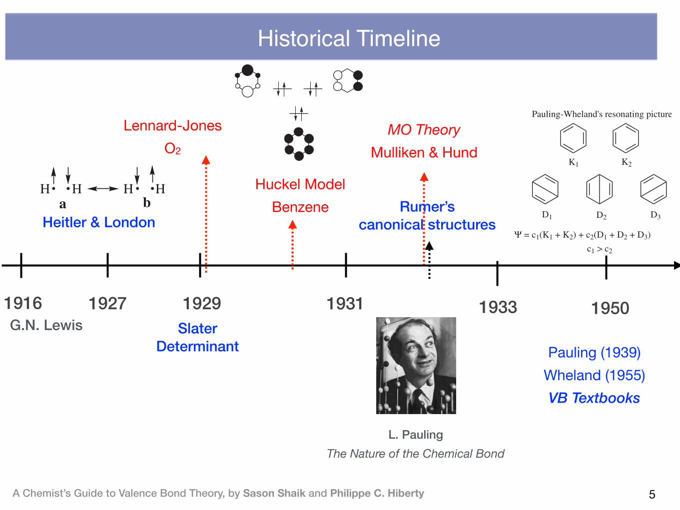
The wave function is always half-covalent and half-ionic, irrespective of distances!!
σ * = χa − χbσ = χa + χb
ΨMO = σ σ = χaχb − χaχb( )+ χaχa + χbχb( )HL
VB
MO
Ionic
10
Bridge Between MO and VB Theory
The wave function is always half-covalent and half-ionic, irrespective of distances!!
ΨMO = σ σ = χaχb − χaχb( )+ χaχa + χbχb( )HL Ionic
Ψ*= σ uσ u = − χaχb − χaχb( )+ χaχa + χbχb( )
ΨMO−CI = c1 σσ − c2 σ uσ u
= (c1 + c2 ) χaχb − χaχb( )+ (c1 − c2 ) χaχa + χbχb( ) (c1 + c2 ) = λ; (c1 − c2 ) = µ
HL Ionic
Both theories, when properly implemented, are correct and mutually transformable
11
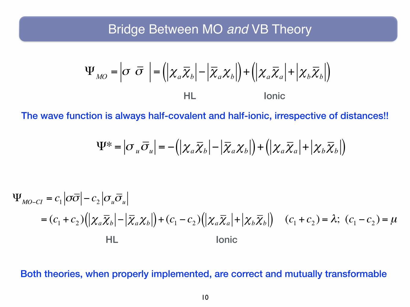
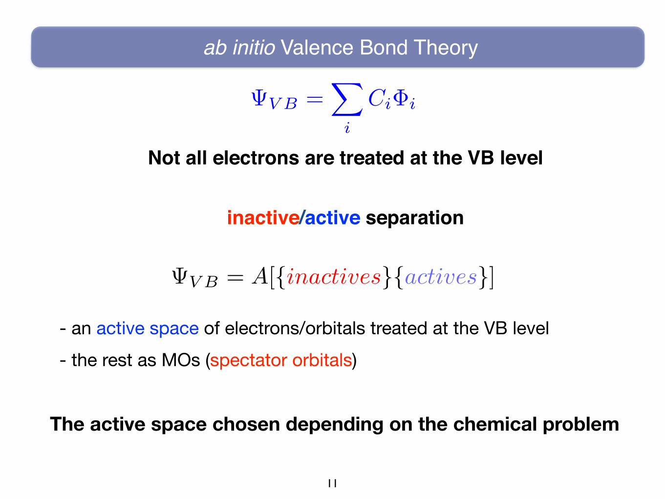
ab initio Valence Bond Theory
V B =X
i
Ci�i
Not all electrons are treated at the VB level
inactive/active separation
- an active space of electrons/orbitals treated at the VB level - the rest as MOs (spectator orbitals)
V B = A[{inactives}{actives}]
The active space chosen depending on the chemical problem

12
ab initio Valence Bond Theory
How many possible VB structures do we have?
Example: the π system of benzene 6 electrons, 6 centres
V B =X
i
Ci�i

13
ab initio Valence Bond Theory
Rumer’s rule for a covalent n-centre/n-electron system:
1. Put the orbitals around an imaginary circle
2. Crossing bonds are not allowed
14
ab initio Valence Bond Theory
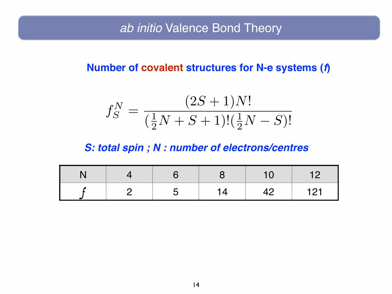
Number of covalent structures for N-e systems (f)
fNS =
(2S + 1)N !
( 12N + S + 1)!( 12N � S)!
N 4 6 8 10 12f 2 5 14 42 121
S: total spin ; N : number of electrons/centres

15
ab initio Valence Bond Theory
1.Choose a distribution of charges
2. Apply Rumer’s rules on the rest
3.Choose another distribution of charges...
Rumer’s rule for N-e/N-c ionic structures
4. Another one …
16
ab initio Valence Bond Theory
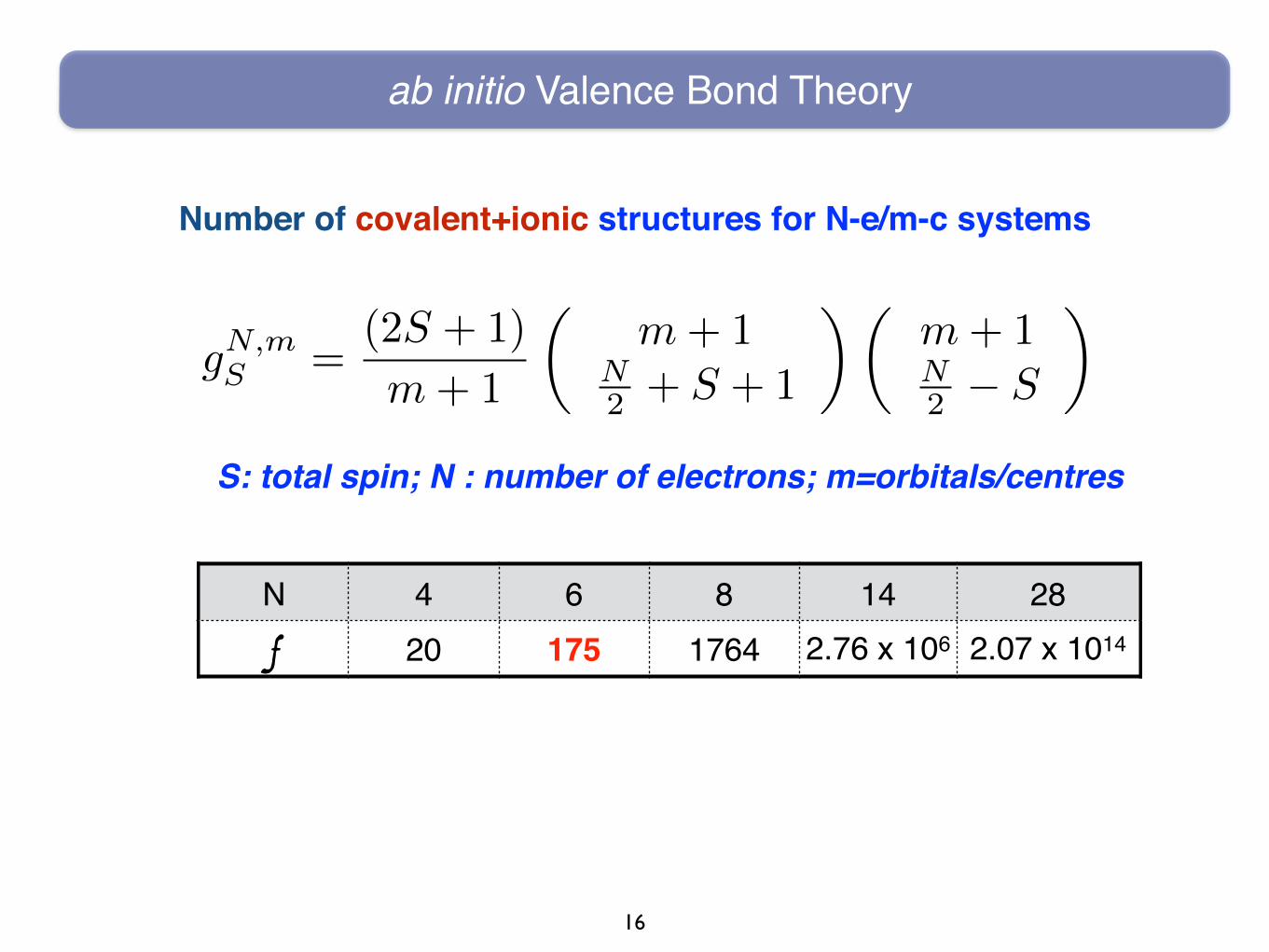
Number of covalent+ionic structures for N-e/m-c systems
N 4 6 8 14 28f 20 175 1764 2.76 x 10⁶ 2.07 x 10¹⁴
gN,mS =
(2S + 1)
m+ 1
✓m+ 1
N2 + S + 1
◆✓m+ 1N2 � S
◆
S: total spin; N : number of electrons; m=orbitals/centres

17
Describing Chemical SN2 Reactions
V B = A[{inactives}{actives}]
C Y
H
HH
X
Cl- + CH3 – Cl Cl – CH3 + Cl-

18
Describing Chemical SN2 Reactions
C Y
H
HH
X
Cl- + CH3 – Cl Cl – CH3 + Cl-
22 core electrons (1s, 2s and 2p of Cl, 1s of C) described by 11 doubly occupied MOs.
4 active valence electrons will occupy VB vectors localised on the corresponding fragments.

19
Describing Chemical SN2 Reactions
4-e/3-orbital/centre VB system g4,30 =1
4
✓43
◆✓42
◆
C Y
H
HH
X
Depending on identity of nucleophile (Nu) and leaving group (LG) overall number of valence electrons can vary.
There will always be at least four active electrons (i.e. electrons involved in the bond breaking/forming)

20
VB Description of SN2 Reaction
6 VB structures
(5)
(4)
X H3C Y+ +
Y+X + + CH3X H3C Y
(3)
(1)
(2)
+
X CH3 Y+
Y+X + CH3 X C Y++(6)

(5)
(4)
X H3C Y+ +
Y+X + + CH3X H3C Y
(3)
(1)
(2)
+
X CH3 Y+
Y+X + CH3 X C Y++(6)
21
VB Description of SN2 Reaction
6 VB structures
|xx(cy + cy)|
|cc(xy + xy)|
|yy(xc+ cx)| |xxcc|
|xxyy|
|ccyy|
22
C Y
H
HH
X
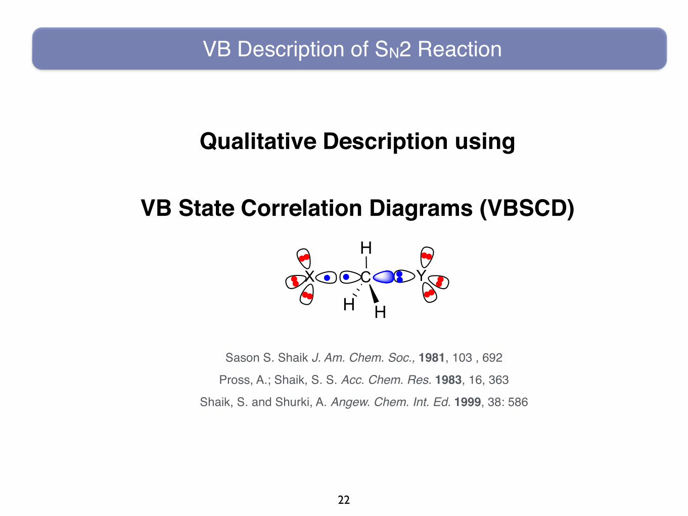
Qualitative Description using
VB State Correlation Diagrams (VBSCD)
VB Description of SN2 Reaction
Sason S. Shaik J. Am. Chem. Soc., 1981, 103 , 692
Pross, A.; Shaik, S. S. Acc. Chem. Res. 1983, 16, 363
Shaik, S. and Shurki, A. Angew. Chem. Int. Ed. 1999, 38: 586

23
C Y
H
HH
X
R = |xx(cy + cy)|
deformation toward P
RS in the PS geometry
VB Description of SN2 Reaction
ReactantX (H3C Y)+
E X CH3 Y

24
C Y
H
HH
X
R = |xx(cy + cy)|
VB Description of SN2 Reaction
Reactant
RS in the PS geometry
P = |yy(xc+ cx)|Product
PS in the RS geometry
X CH3 Y+
X CH3 Y+
X H3C Y+
E X CH3 Y

25
RS in the PS geometry PS in the RS geometry
G = I⇤X �A⇤C � Y
VB Description of SN2 Reaction
R = |xx(cy + cy)|Reactant
P = |yy(xc+ cx)|Product
X CH3 Y+
X CH3 Y+
X H3C Y+
E X CH3 Y

26
a barrier formation is described as a result of avoided crossing between two state curves
B: resonance energy
VB Description of SN2 Reaction
X CH3 Y+
X CH3 Y+
X H3C Y+
E X CH3 Y

27
a barrier formation is described as a result of avoided crossing between two state curves
B: resonance energy
VB Description of SN2 Reaction
ground state
excited state
X CH3 Y+
X CH3 Y+
X H3C Y+
E X CH3 Y

28
B: resonance energy of the TS due to VB mixing
VB Description of SN2 Reaction
�G = fG�B
G
ΔE=fG
P
E
R
P*R*
ground state
excited state
G: R→R* is an excited diabatic state
R*

29
VB Description of SN2 Reaction
Principles• Two-state (VBSCD) vs. multi-state diagrams (VBCMD) :
Barrier Stepwise
R and P mix to form the barrier and the TS for an
elementary process
The intermediate has a different electronic structure than R and P
(«internal catalysis»)

30
• General Applicability: Nucleophilic, electrophilic, radical,
pericyclic reactions …
• Simple: could be applied «on the back of en envelope»
• Insightful: allows to create order among great families of
reactions
• Qualitative reasonings: a few rules and elementary interactions
- quantitive proof : by high level VB calculations
VB Description of SN2 Reaction

31
C Y
H
HH
X
Quantitative Description
VB Description of SN2 Reaction
32
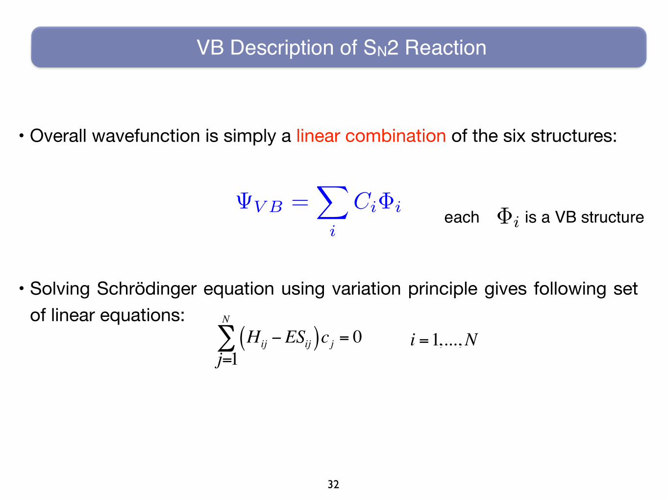
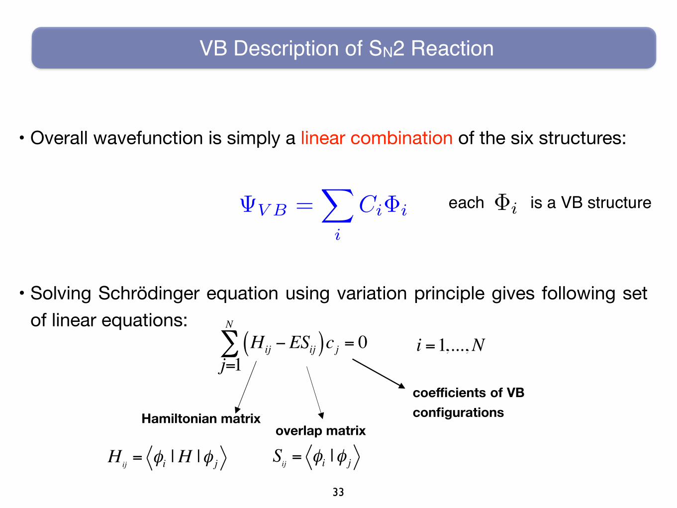
• Overall wavefunction is simply a linear combination of the six structures:
• Solving Schrödinger equation using variation principle gives following set of linear equations:
Hij −ESij( )cj = 0j=1
N
∑ i =1,...,N
VB Description of SN2 Reaction
each is a VB structure �i V B =
X
i
Ci�i
33
• Overall wavefunction is simply a linear combination of the six structures:
• Solving Schrödinger equation using variation principle gives following set of linear equations:
Hij −ESij( )cj = 0j=1
N
∑ i =1,...,N
VB Description of SN2 Reaction
each is a VB structure �i V B =X
i
Ci�i
Hamiltonian matrixoverlap matrix
coefficients of VB configurations
Sij = φi |φ jHij = φi |H |φ j

34
VB Description of SN2 Reaction
X H3C Y(1)
(5)
(4)
(3)
(2)
+
X CH3 Y+
Y+X + CH3
X H3C Y+ +
Y+X + CH3
Shurki et al. Chem. Soc. Rev., 2015, 44, 1037

35
Softwares to Run ab initio VB
Program Capabilities Website Comments Reference
V2000
VBSCF, BOVB, VBCI,
SCVB, CASVB GVB
http://www.scinetec.com
Integrated into GAMESS
McWeeny and coworkers
TURTLE VBSCFhttp://tc5.chem.uu.nl/
ATMOL/turtle/turtle_main.html
Integrated into GAMESS-UK van Lenthe et al.
XMVB
VBSCF, BOVB, VBCI, VBPT2,
DFVB, VBPCM, VBEFP, VBEFP/
PCM
http://ftcc.xmu.edu.cn/xmvb/index.html
Integrated into GAMESS
Wu and coworkers

36
ab initio Valence Bond Theory
Adds on for Condense Phases:
VBPCM VBSM VB/MM
+PCM +SM +MM
VBCI BOVB
VBCI
VBSCF
Breathing OrbitalsCI
PT2
Different ways to introduce full correlation
Wu et al. Chem. Rev., 2011, 111, 7557
Localised orbitals

37
VBSCF Method
• Orbitals and Ci coefficients of different structures are optimised simultaneously, leading to self-consistent field type wave function.
• VBSCF basically multi-configuration SCF method with the added advantage of utilising chemically interpretable configurations.
• Analogous to MO-based CASSCF. However, VBSCF uses fewer structures and localised non-orthogonal orbitals.
0 =X
k
ak�k where each Φi is a VB structure
GVB, SCVB ~ equivalent to VBSCF
F•—•F F–F+ F+F–
Coefficients Ci and orbitals optimized simultaneously (like MCSCF)
All orbitals are optimized (active as well as spectator ones)
How does one calculate VB wave functions with localized orbitals ?
!
"VB
= Ci
i
# $i where each Φi is a VB structure
The VBSCF method (Balint-Kurti & van Lenthe)
Example: the F2 molecule
F F•••
••
••
••••
••
• F F••
••
••
••••
••
F F
••
••
••••
••
C1 + C2 + C2•• ••••XX X XXC1 + C2 + C2X

38
Accuracy of the various methods
Computational errors of BD energies relative to the FCI method
Wu et al. Chem. Rev., 2011, 111, 7557
What is VBSCF missing?

39
VBSCF Method
GVB, SCVB ~ equivalent to VBSCF
F•—•F F–F+ F+F–
Coefficients Ci and orbitals optimized simultaneously (like MCSCF)
All orbitals are optimized (active as well as spectator ones)
How does one calculate VB wave functions with localized orbitals ?
!
"VB
= Ci
i
# $i where each Φi is a VB structure
The VBSCF method (Balint-Kurti & van Lenthe)
Example: the F2 molecule
F F•••
••
••
••••
••
• F F••
••
••
••••
••
F F
••
••
••••
••
C1 + C2 + C2•• ••••
The same set of AOs is used for all VB structures…. 0 =X
k
ak�k
Optimised for a mean neutral situation
XX X XXC1 + C2 + C2X

GVB, SCVB ~ equivalent to VBSCF
F•—•F F–F+ F+F–
Coefficients Ci and orbitals optimized simultaneously (like MCSCF)
All orbitals are optimized (active as well as spectator ones)
How does one calculate VB wave functions with localized orbitals ?
!
"VB
= Ci
i
# $i where each Φi is a VB structure
The VBSCF method (Balint-Kurti & van Lenthe)
Example: the F2 molecule
F F•••
••
••
••••
••
• F F••
••
••
••••
••
F F
••
••
••••
••
C1 + C2 + C2•• ••••
40
VBSCF Method
GVB, SCVB ~ equivalent to VBSCF
F•—•F F–F+ F+F–
Coefficients Ci and orbitals optimized simultaneously (like MCSCF)
All orbitals are optimized (active as well as spectator ones)
How does one calculate VB wave functions with localized orbitals ?
!
"VB
= Ci
i
# $i where each Φi is a VB structure
The VBSCF method (Balint-Kurti & van Lenthe)
Example: the F2 molecule
F F•••
••
••
••••
••
• F F••
••
••
••••
••
F F
••
••
••••
••
C1 + C2 + C2•• ••••
The same set of AOs is used for all VB structures…. 0 =X
k
ak�k
Optimised for a mean neutral situation
XX XX XXC1 + C2 + C2
XX X XXC1 + C2 + C2X
Better Representation

41
Improvements on VBSCF Method
BOVB removes average field restriction of VBSCF. The orbitals are variationally optimised with the freedom to be different for different VB structures.
BOVB
- Orbitals for F•—•F will be the same as VBSCF
- Orbitals for ionic structures will be much improved
Wu et al. Chem. Rev., 2011, 111, 7557

42
Improvements on VBSCF Method
Iteration De(kcal) F•–•F F+F– ↔ F–F+
Classical VB -4.6 0.813 0.187
GVB,VBSCF ~ 15 0.768 0.232
BOVB 1 24.6 0.731 0.269
2 27.9 0.712 0.288
3 28.4 0.709 0.291
4 28.5 0.710 0.290
5 28.6 0.707 0.293
Full CI 30-33
Test case: the dissociation of F2
F–F F• + F• ΔE
Calculation of ∆E for F-F=1.43Å, 6-31G(d) basis:
BOVB brings that part of dynamic correlation that varies in the process Philippe C. Hiberty

43
Improvements on VBSCF Method
1. Start from VBSCF
VBCI
0 =X
k
ak�k
3. Improve " by post-VBSCF configuration interaction: �CIµ =
X
k
Ckµ�
kµ
All are excitations that correspond to the same VB structure
�CIµ is a multi-determinant description of a unique VB structure.
�kµ
4. Do the configuration interaction:
2. For each Φk define a set of strictly localised virtual orbitals
BV CI =X
µ
CCIµ �CI
µ

44
Incorporation of Solvent Effects
(H0 +VR )ΨVB = EΨVB
VBPCM combined VB approach with PCM.
Interactions between solute charges and polarised electric field of solvent considered by embedding an interaction potential into the VB Hamiltonian:
VBSM uses SMX (currently X=6) to account for solvation.
solvent-solute electrostatic interactions are described by the generalised born (GB) approximation, with self-consistent solute charges.
environmentisdescribedasbeinghomogenous

45
VB/MM Calculations
For meaningful description of environment, need to move to hybrid QM/MM description
How to deal with coupling between QM and MM parts?
• Simplest approach: QM and MM parts do not polarise each other, only mechanical embedding considered.
• MM point charges polarise QM region in process referred to as electrostatic embedding.
Shurki et al. J. Phys. Chem. B, 2010, 114, 2212

46
VB/MM Calculations
Hij −ESij( )cj = 0j=1
N
∑ i =1,...,N
Hamiltonian matrixoverlap matrix
coefficients of VB configurations
Sij = φi |φ jHij = φi |H |φ j
Diagonal elements: energy of the respective VB configuration
QM energy of configuration Φiinteraction energy of Φi configuration with its surrounding
Hii = H0ii +Hint
ii
47
VB/MM Calculations
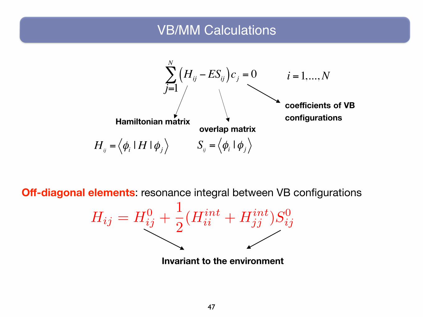
Hij −ESij( )cj = 0j=1
N
∑ i =1,...,N
Hamiltonian matrixoverlap matrix
coefficients of VB configurations
Sij = φi |φ jHij = φi |H |φ j
Off-diagonal elements: resonance integral between VB configurations
Invariant to the environment
Hij = H0ij +
1
2(Hint
ii +Hintjj )S0
ij
48
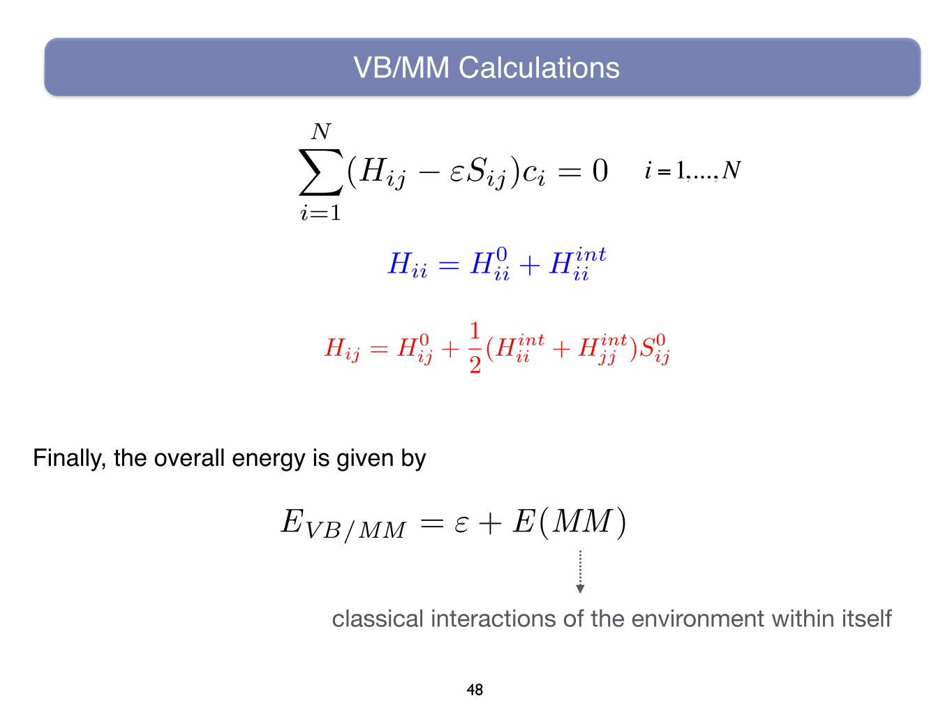
VB/MM Calculations
i =1,...,N
Finally, the overall energy is given by
Hij = H0ij +
1
2(Hint
ii +Hintjj )S0
ij
Hii = H0ii +Hint
ii
classical interactions of the environment within itself
EVB/MM = "+ E (MM )
NX
i=1
(Hij � "Sij)ci = 0

49
VB/MM Calculations
i =1,...,N
Finally, the overall energy is given by
Hij = H0ij +
1
2(Hint
ii +Hintjj )S0
ij
Hii = H0ii +Hint
ii
classical interactions of the environment within itself
EVB/MM = "+ E (MM )
NX
i=1
(Hij � "Sij)ci = 0