Using Unitized Uncertainty Using Unitized Uncertainty Using Unitized Uncertainty Using Unitized Uncertainty Using Unitized Uncertainty Using Unitized Uncertainty Distributions in ACEITDistributions in ACEIT

Using Unitized Uncertainty Using Unitized Uncertainty Distributions in ACEITDistributions in ACEIT

ACEIT Users WorkshopFebruary 1-2, 2010

Jeff McDowell

Pending: Approved for Public Release

OutlineOutlineOutlineOutline

Background and DefinitionSimple Example ExerciseSimple Example ExerciseRefined DefinitionCatalogExpanded ExerciseBest PracticesSummaryy

01 February 2011 Approved for Public Release 2

Background and DefinitionBackground and DefinitionBackground and DefinitionBackground and DefinitionBackground and DefinitionBackground and DefinitionBackground and DefinitionBackground and Definition

01 February 2011 Approved for Public Release 3

ChallengeChallengeChallengeChallenge

There is an ever-present desire for general-purpose distributions to apply to WBSpurpose distributions to apply to WBS elements by commodity.Ongoing research sponsored by the AirOngoing research sponsored by the Air Force Cost Analysis Agency will meet this need.Product will consist of a metrics manual of unitized distributions organized by commodity and WBS.

01 February 2011 Approved for Public Release 4

Uncertainty Modeling Uncertainty Modeling AlgebraicallyAlgebraically

Uncertainty Modeling Uncertainty Modeling AlgebraicallyAlgebraicallyg yg yg yg y

Given:Cost Element = Your MethodologyCost Element Point Estimate = Your Methodology

Its uncertainty can then be expressed:Cost Element Uncertainty = f(Your Methodology, Distribution Shape, Distribution Parameters)

Situation-specificNot Reusable

01 February 2011 Approved for Public Release 5

Unitized Distribution:Unitized Distribution:Short DefinitionShort Definition

Unitized Distribution:Unitized Distribution:Short DefinitionShort Definition

A distribution with a center value of one.

01 February 2011 Approved for Public Release 6

A Simple ExampleA Simple ExampleA Simple ExampleA Simple ExampleA Simple ExampleA Simple ExampleA Simple ExampleA Simple Example

01 February 2011 Approved for Public Release 7

Exercise:Exercise:Estimate the Cost of LunchEstimate the Cost of Lunch

Exercise:Exercise:Estimate the Cost of LunchEstimate the Cost of Lunch

Range of Outcomes

01 February 2011 Approved for Public Release 8

Range of Outcomes

Conceptual Cost of LunchConceptual Cost of LunchConceptual Cost of LunchConceptual Cost of Lunch

Most Likely = $5 00Most Likely = $5.00

High Bound= $10.00

$Mean = (min + mode + max)/3Mean = (4 + 5+ 10)/3 = 6 333

01 February 2011 Approved for Public Release 9

Low Bound= $4.00 Mean = (4 + 5+ 10)/3 = 6.333Std Dev = sqrt((min2 + mode2 + max2 –min*mode – min*max – mode*max)/18)Std Dev = sqrt((42 + 52 + 102 – 4*5 – 4*10 –5*10)/18) = 1.312

Algebraic Cost of LunchAlgebraic Cost of LunchAlgebraic Cost of LunchAlgebraic Cost of Lunch

Given:Lunch = 5 00LunchPoint Estimate = 5.00

Its uncertainty can then be expressed:LunchUncertainty = f(Triangular, Low=4.00, ML=5.00, High=10.00)

01 February 2011 Approved for Public Release 10

Modeled Cost of LunchModeled Cost of LunchModeled Cost of LunchModeled Cost of Lunch

All well and good, but:Situation-specificpNot Reusable

01 February 2011 Approved for Public Release 11

New ExercisesNew ExercisesNew ExercisesNew Exercises

Estimate the Cost of Breakfast

$4.00

Estimate the Cost of Dinner

$15.00

Range of Outcomes??? ???

01 February 2011 Approved for Public Release 12

Range of Outcomes??? ???

Algebraic Cost of Breakfast Algebraic Cost of Breakfast and Dinnerand Dinner

Algebraic Cost of Breakfast Algebraic Cost of Breakfast and Dinnerand Dinner

Given:Breakfast = 4 00BreakfastPoint Estimate = 4.00DinnerPoint Estimate = 15.00

Insufficient information to express their uncertainty:BreakfastUncertainty = f(PE=4, Shape Unknown, Bounds Unknown)DinnerUncertainty = f(PE=15, Shape Unknown,

01 February 2011 Approved for Public Release 13

Bounds Unknown)

Solution: Borrow Shape and Solution: Borrow Shape and Bounds From a Known CaseBounds From a Known CaseSolution: Borrow Shape and Solution: Borrow Shape and Bounds From a Known CaseBounds From a Known Case

Cannot use the known case’s parameters directlyCan only use their relative valuesUse Linear Transform: Divide through by the central value

Most Likely = $5.00 / $5.001 00= 1.00

High Bound= $10.00 / $5.00= 2.00

L B d $4 00 / $5 00Low Bound= $4.00 / $5.00= 0.80

01 February 2011 Approved for Public Release 14

Unitized DistributionUnitized DistributionUnitized DistributionUnitized Distribution

Most Likely = 1 00Most Likely = 1.00

High Bound = 2.00

01 February 2011 Approved for Public Release 15

Low Bound = 0.80

Note Other Characteristics Note Other Characteristics Also Scale LinearlyAlso Scale Linearly

Note Other Characteristics Note Other Characteristics Also Scale LinearlyAlso Scale Linearlyyyyy

Mean = (min + mode + max)/3Mean = (4 + 5+ 10)/3 = 6.333Std Dev = sqrt((min2 + mode2 + max2 –min*mode – min*max – mode*max)/18)Std Dev = sqrt((42 + 52 + 102 – 4*5 – 4*10 –

Mean = (min + mode + max)/3Mean = (0.8 + 1 + 2)/3 = 1.267Std Dev = sqrt((min2 + mode2 + max2 –min*mode – min*max – mode*max)/18)Std Dev = sqrt((0.82 + 12 + 22 – 0.8*1 –

Mean = 6.333 / 5 = 1.267

Std Dev = 1.312 / 5 = 0.262

Most Likely = $5.00 / $5.001 00

5*10)/18) = 1.312 0.8*2 – 1*2)/18) = 0.262

= 1.00

High Bound= $10.00 / $5.00= 2.00

L B d $4 00 / $5 00Low Bound= $4.00 / $5.00= 0.80

01 February 2011 Approved for Public Release 16

Algebraic Cost of Breakfast Algebraic Cost of Breakfast and Dinnerand Dinner

Algebraic Cost of Breakfast Algebraic Cost of Breakfast and Dinnerand Dinner

Given:BreakfastPoint Estimate = 4.00BreakfastPoint Estimate 4.00LunchPoint Estimate = 5.00 DinnerPoint Estimate = 15.00

Using Unitized Distributions to express uncertainty:BreakfastUncertainty = (PE=4) * Triangular (0.80, 1.00, 2.00)LunchUncertainty = (PE=5) * Triangular (0.80, 1.00, 2.00) Dinner = (PE=15) * Triangular (0 80 1 00 2 00)DinnerUncertainty = (PE=15) * Triangular (0.80, 1.00, 2.00)

01 February 2011 Approved for Public Release 17

Modeled Cost of MealsModeled Cost of MealsModeled Cost of MealsModeled Cost of Meals

01 February 2011 Approved for Public Release 18

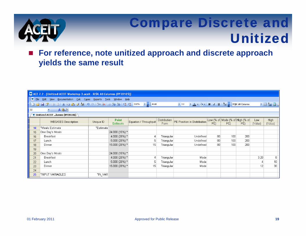
Compare Discrete and Compare Discrete and UnitizedUnitized

Compare Discrete and Compare Discrete and UnitizedUnitized

For reference, note unitized approach and discrete approach yields the same result

01 February 2011 Approved for Public Release 19

Algebraic Using Unitized Algebraic Using Unitized DistributionsDistributions

Algebraic Using Unitized Algebraic Using Unitized DistributionsDistributions

Given:Cost Element = Your MethodologyCost Element Point Estimate = Your Methodology

Its uncertainty can then be expressed:Cost Element Uncertainty = f(Your Methodology, Distribution Shape,

Distribution Parameters)Distribution Parameters)Cost Element Uncertainty =

Your Methodology * Unitized Distribution

01 February 2011 Approved for Public Release 20

Refined DefinitionRefined DefinitionRefined DefinitionRefined DefinitionRefined DefinitionRefined DefinitionRefined DefinitionRefined Definition

01 February 2011 Approved for Public Release 21

DefinitionDefinitionDefinitionDefinition

A unitized distribution has a center value of oneone.A unitized distribution is designed to be modeled as a multiplier of point estimatesmodeled as a multiplier of point estimates. A unitized distribution is useful when discrete bounds or distribution shape isdiscrete bounds or distribution shape is unknown.

01 February 2011 Approved for Public Release 22

Catalog of Unitized Catalog of Unitized Catalog of Unitized Catalog of Unitized ggDistributionsDistributionsggDistributionsDistributions

01 February 2011 Approved for Public Release 23

CatalogCatalogCatalogCatalog

The AFCAA Cost Risk and Uncertainty Analysis Metrics Manual (CRUAMM) willAnalysis Metrics Manual (CRUAMM) will provide guidelines and empirical metrics for developing cost uncertainty analysesA Catalog of Empirically-Based Unitized Uncertainty Distributions

Sample My Point Estimate is the:Dataset CV Mean Median ModeWBS # and Stratification Class nn Lognormal (Mean, Std Dev) Lognormal (Mean, Std Dev) Lognormal (Mean, Std Dev)WBS # and Stratification Class nn Normal (Mean, Std Dev) Normal (Mean, Std Dev) Normal (Mean, Std Dev)WBS # and Stratification Class nn Triangular (Low, Mode, High) Triangular (Low, Mode, High) Triangular (Low, Mode, High)WBS # and Stratification Class nn Beta (Low, High, Alpha, Beta) Beta (Low, High, Alpha, Beta) Beta (Low, High, Alpha, Beta)

01 February 2011 Approved for Public Release 24

Catalog and ACEIT Catalog and ACEIT InstructionsInstructions

Catalog and ACEIT Catalog and ACEIT InstructionsInstructions

Sample My Point Estimate is the:Dataset CV Mean Median ModeWBS # and Stratification Class nn Normal (Mean, Std Dev) Normal (Mean, Std Dev) Normal (Mean, Std Dev)WBS # and Stratification Class nn Lognormal (Mean, Std Dev) Lognormal (Mean, Std Dev) Lognormal (Mean, Std Dev)WBS # and Stratification Class nn Triangular (Low, Mode, High) Triangular (Low, Mode, High) Triangular (Low, Mode, High)WBS # and Stratification Class nn Beta (Low, High, Alpha, Beta) Beta (Low, High, Alpha, Beta) Beta (Low, High, Alpha, Beta)

Legend:L = Low (Value) or Low (% of PE)H = High Value or High (% of PE)Note that you should also enter Low Percentile and High Percentile when entering Low and/or High values.Sp = SpreadSk = SkewASE = Adjusted SECV = Coefficient of VariationSD = Standard DeviationSD Standard DeviationMode = Most likely valueMode% = Confidence probability of the mode

Note 1: For the Triangular distribution, enter the confidence level of the mode in the Mode % column. The confidence must be between 0.0 and 1.0. Enter the PE variation with fixed range in the Spread field.

Note 2:For the Uniform distribution, enter the confidence level of the input cost in theconfidence level of the input cost in the Mode% column. The confidence must be between 0.0 and 1.0. Even more specifications for Uniform are allowed. See help topic for Uniform for the complete list.

Note 3:For Weibull distribution, partial inputs have different meanings depending on the fields entered. For example, if spread is given alone, it must be a preset selection (i.e., L, M or H). Values for Scale (b) must be between 0.0001 and 30000.0. Range for Shape (alpha) is 1 0 to 300 0 For the Priority 4

01 February 2011 Approved for Public Release 25

Source: ACEIT Help

(alpha) is 1.0 to 300.0. For the Priority 4 case, the Low Percentile is always 0.0%, and the Skew is the confidence of the mode. This value must be between 0.0 and 0.5. See Weibull Distribution for more information.

Use the Input All Use the Input All Form’s Form’s RI$K RI$K Tab Tab to to Enter Enter Distribution InformationDistribution Information

Use the Input All Use the Input All Form’s Form’s RI$K RI$K Tab Tab to to Enter Enter Distribution InformationDistribution Information

Advanced mode of the Input All From RI$K tab Steps in defining a distribution:

S 1 E h h dStep 1: Enter the method or throughput for the row.Step 2: Select a distribution type – What is the shape of the uncertainty you want to model?Step 3: Enter the Point Estimate (PE) Position –What does the point estimate represent (i.e. the mode, low, (high, median, unknown)?Step 4: Indentify the remaining shape of the distribution – This will vary depending on the PE position p g pand the bound information you have available to you. When the distribution is fully specified the status will say Complete.

01 February 2011 Approved for Public Release 26

Source: RI$K Training 12 Apr 2010Copyright © Tecolote Research, Inc. April 2010

An Expanded ExampleAn Expanded ExampleAn Expanded ExampleAn Expanded ExampleAn Expanded ExampleAn Expanded ExampleAn Expanded ExampleAn Expanded Example

01 February 2011 Approved for Public Release 27

ExampleExampleExampleExample

Begin with a point estimate

01 February 2011 Approved for Public Release 28

Using a Catalog of Unitized Using a Catalog of Unitized DistributionsDistributions

Using a Catalog of Unitized Using a Catalog of Unitized DistributionsDistributions

Locate appropriate tableSelect row for your WBS and ClassSelect column for the your point estimate interpretation

Sample My Point Estimate is the:Dataset CV Mean Median ModeSensor, IR 0.490 Normal (1.000, 0.4872) Normal (1.000, 0.4872) Normal (1.000, 0.4872)Sensor, MMW 0.349 Normal (1.000, 0.3490) Normal (1.000, 0.3490) Normal (1.000, 0.3490)Sensor, Laser 0.670 Normal (1.000, 0.6732) Normal (1.000, 0.6732) Normal (1.000, 0.6732)Sensor, Tri‐mode 0.855 Beta (0.28, 5.72, 0.44, 2.89) Beta (0.82, 7.42, 0.44, 2.89) Beta (1.00, 15.07, 0.44, 2.89)

Sample My Point Estimate is the:Dataset CV Mean Median ModeStructure, Air, Composite 0.560 Lognormal (1.0000, 0.6408) Lognormal (1.1969, 0.7602) Lognormal (6.1976, 1.1691)Structure, Ground, Composite 0.981 Lognormal (1.0000, 1.6189) Lognormal (1.9029, 3.0807) Lognormal (6.8904, 11.1551)Structure, Air, Aluminum 1.320 Triangular (0.00, 0.0185, 2.9815) Triangular (0.00, 0.0210, 3.3888) Triangular (0.00, 1.0000, 16.1310)Structure, Ground, Aluminum 0.125 Normal (1.0000, 0.1256) Normal (1.0000, 0.1256) Normal (1.0000, 0.1256)

Sample My Point Estimate is the:Dataset CV Mean Median ModeC i i UHF XMTR 0 526 T i l (0 00 0 6585 2 3515) T i l (0 00 0 6910 2 5088) T i l (0 00 1 0000 3 6310)Communication, UHF XMTR 0.526 Triangular (0.00, 0.6585, 2.3515) Triangular (0.00, 0.6910, 2.5088) Triangular (0.00, 1.0000, 3.6310)Communication, VHF Ground 0.567 Triangular (0.00, 0.0185, 2.9815) Triangular (0.00, 0.0210, 3.3888) Triangular (0.00, 1.0000, 16.1310)Communication, UHF Air 0.350 Normal (1.000, 0.3490) Normal (1.000, 0.3490) Normal (1.000, 0.3490)Communication, UHF Sea 0.423 Triangular (0.00, 1.4385, 1.5715) Triangular (0.00, 1.3610, 1.4788) Triangular (0.00, 1.0000, 1.0910)

Sample My Point Estimate is the:Dataset CV Mean Median Mode

01 February 2011 Approved for Public Release 29

Dataset CV Mean Median ModePower, Battery, NiCd 0.594 Beta (0.19, 2.33, 0.87, 1.44) Beta (0.21, 2.55, 0.87, 1.44) Beta (0.19, 12.39, 0.87, 1.44)Power, Battery, Li 0.919 Beta (0.07, 3.87, 0.56, 1.74) Beta (0.11, 5.47, 0.56, 1.74) Beta (0.07, 52.02, 0.56, 1.74)Power, Networks 0.801 Beta (0.07, 2.72, 0.66, 1.20) Beta (0.08, 3.20, 0.66, 1.20) Beta (1.00, 38.65, 0.66, 1.20)Power, Generator 0.600 Lognormal (1.0000, 0.6408) Lognormal (1.1969, 0.7602) Lognormal (6.1976, 1.1691)

Input Input All All Form: LognormalForm: LognormalInput Input All All Form: LognormalForm: Lognormal

Steps in defining a distribution:

S 1 E h h dStep 1: Enter the method or throughput for the row.Step 2: Select a distribution type – What is the shape of the uncertainty you want to model?Step 3: Enter the Point Estimate (PE) Position –Use “Undefined” for Unitized Distributions.

Step 4: Indentify the remaining shape of the distribution – This will vary depending on the PE positiondepending on the PE position and the bound information you have available to you. When the distribution is fully specified the status will say Complete.

01 February 2011 Approved for Public Release 30

y p

Input Input All All Form: NormalForm: NormalInput Input All All Form: NormalForm: Normal

Steps in defining a distribution:

S 1 E h h dStep 1: Enter the method or throughput for the row.Step 2: Select a distribution type – What is the shape of the uncertainty you want to model?Step 3: Enter the Point Estimate (PE) Position –Use “Undefined” for Unitized Distributions.

Step 4: Indentify the remaining shape of the distribution – This will vary depending on the PE positiondepending on the PE position and the bound information you have available to you. When the distribution is fully specified the status will say Complete.

01 February 2011 Approved for Public Release 31

y p

Input Input All All Form: TriangularForm: TriangularInput Input All All Form: TriangularForm: Triangular

Steps in defining a distribution:

S 1 E h h dStep 1: Enter the method or throughput for the row.Step 2: Select a distribution type – What is the shape of the uncertainty you want to model?Step 3: Enter the Point Estimate (PE) Position –Use “Undefined” for Unitized Distributions.

Step 4: Indentify the remaining shape of the distribution – This will vary depending on the PE position Note: Low and High Percentile at absolutedepending on the PE position and the bound information you have available to you. When the distribution is fully specified the status will say Complete.

01 February 2011 Approved for Public Release 32

y p

Input Input All All Form: BetaForm: BetaInput Input All All Form: BetaForm: Beta

Steps in defining a distribution:

S 1 E h h dStep 1: Enter the method or throughput for the row.Step 2: Select a distribution type – What is the shape of the uncertainty you want to model?Step 3: Enter the Point Estimate (PE) Position –Use “Undefined” for Unitized Distributions.

Step 4: Indentify the remaining shape of the distribution – This will vary depending on the PE position Note: Low and High Percentile at absolute

N t Al h d B t t d 1depending on the PE position and the bound information you have available to you. When the distribution is fully specified the status will say Complete.

Note: Alpha and Beta entered as +1

01 February 2011 Approved for Public Release 33

y p

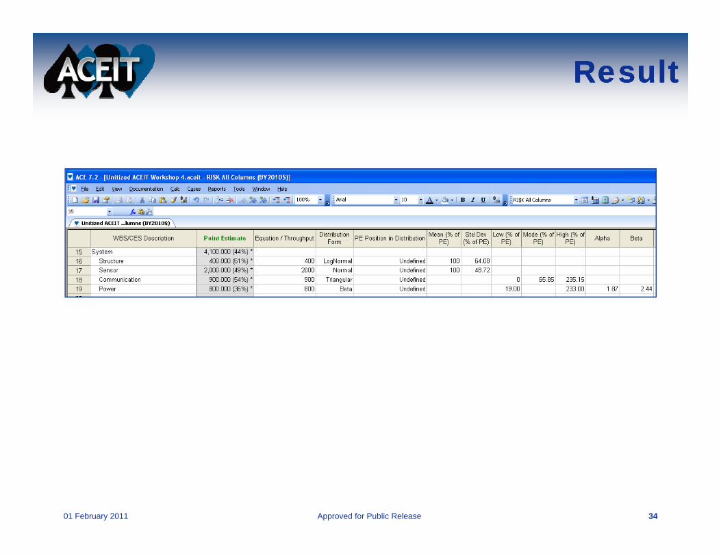
ResultResultResultResult

01 February 2011 Approved for Public Release 34

Alternate Point Estimate Alternate Point Estimate PositionsPositions

Alternate Point Estimate Alternate Point Estimate PositionsPositions

Each of the preceding four elements p gassumed the point estimate was the mean.

The next two elements assume the point estimate is the Median and the Mode.

01 February 2011 Approved for Public Release 35

Input Input All All Form: Lognormal With Form: Lognormal With Median Point EstimateMedian Point Estimate

Input Input All All Form: Lognormal With Form: Lognormal With Median Point EstimateMedian Point Estimate

Steps in defining a distribution:

S 1 E h h dStep 1: Enter the method or throughput for the row.Step 2: Select a distribution type – What is the shape of the uncertainty you want to model?Step 3: Enter the Point Estimate (PE) Position –Use “Undefined” for Unitized Distributions.

Step 4: Indentify the remaining shape of the distribution – This will vary depending on the PE positiondepending on the PE position and the bound information you have available to you. When the distribution is fully specified the status will say Complete.

01 February 2011 Approved for Public Release 36

y p

Input Input All All Form: Lognormal With Form: Lognormal With Mode Point EstimateMode Point Estimate

Input Input All All Form: Lognormal With Form: Lognormal With Mode Point EstimateMode Point Estimate

Steps in defining a distribution:

S 1 E h h dStep 1: Enter the method or throughput for the row.Step 2: Select a distribution type – What is the shape of the uncertainty you want to model?Step 3: Enter the Point Estimate (PE) Position –Use “Undefined” for Unitized Distributions.

Step 4: Indentify the remaining shape of the distribution – This will vary depending on the PE positiondepending on the PE position and the bound information you have available to you. When the distribution is fully specified the status will say Complete.

01 February 2011 Approved for Public Release 37

y p

Best practicesBest practicesBest practicesBest practicesBest practicesBest practicesBest practicesBest practices

01 February 2011 Approved for Public Release 38

Leave the PE Position in Leave the PE Position in Distribution as “Undefined”Distribution as “Undefined”

Leave the PE Position in Leave the PE Position in Distribution as “Undefined”Distribution as “Undefined”

Retain positive control over model inputs

01 February 2011 Approved for Public Release 39

A Bad Practice to AvoidA Bad Practice to AvoidA Bad Practice to AvoidA Bad Practice to Avoid

Tempting idea: Simplify body of your estimate by defining distributions as Input y gVariables.

Not recommended as it results in unintended

01 February 2011 Approved for Public Release 40

Not recommended as it results in unintended correlation.

SummarySummarySummarySummary

Defined and Illustrated Unitized DistributionsDemonstrated How to Use Unitized Distributions in ACEIT

Questions

01 February 2011 Approved for Public Release 41