Using the material-point method to model sea ice dynamicssulsky/papers/SulskyEtAlJGR.pdf · Using...

Using the material-point method to model sea ice

dynamics

Deborah Sulsky,1 Howard Schreyer,2 Kara Peterson,1 Ron Kwok,3 and Max Coon4

Received 25 September 2005; revised 17 August 2006; accepted 2 October 2006; published 22 February 2007.

[1] The material-point method (MPM) is a numerical method for continuum mechanicsthat combines the best aspects of Lagrangian and Eulerian discretizations. The materialpoints provide a Lagrangian description of the ice that models convection naturally. Thusproperties such as ice thickness and compactness are computed in a Lagrangian frame anddo not suffer from errors associated with Eulerian advection schemes, such as artificialdiffusion, dispersion, or oscillations near discontinuities. This desirable property isillustrated by solving transport of ice in uniform, rotational and convergent velocity fields.Moreover, the ice geometry is represented by unconnected material points rather than agrid. This representation facilitates modeling the large deformations observed in theArctic, as well as localized deformation along leads, and admits a sharp representation ofthe ice edge. MPM also easily allows the use of any ice constitutive model. The versatilityof MPM is demonstrated by using two constitutive models for simulations ofwind-driven ice. The first model is a standard viscous-plastic model with two thicknesscategories. The MPM solution to the viscous-plastic model agrees with previouslypublished results using finite elements. The second model is a new elastic-decohesivemodel that explicitly represents leads. The model includes a mechanism to initiate leads,and to predict their orientation and width. The elastic-decohesion model can providesimilar overall deformation as the viscous-plastic model; however, explicit regions ofopening and shear are predicted. Furthermore, the efficiency of MPM with theelastic-decohesive model is competitive with the current best methods for sea icedynamics.

Citation: Sulsky, D., H. Schreyer, K. Peterson, R. Kwok, and M. Coon (2007), Using the material-point method to model sea ice

dynamics, J. Geophys. Res., 112, C02S90, doi:10.1029/2005JC003329.

1. Introduction

[2] Ice dynamics models are used to generate short-termforecasts for waterways [Sayed and Carrieres, 1999], topredict the ice-edge position for offshore operations [Flato,1993] and to understand the global climate in long-termstudies [Maslowski et al., 2001]. A continuum model ofpack ice dynamics involves a mathematical description ofthe physical laws, such as momentum balance. The balancelaws must be augmented by constitutive relations in order todistinguish a particular type of continuum, in this case, ice.The appropriate balance laws for our model are presented insection 2. Constitutive models for the pack ice are presentedin section 4.[3] Once the mathematical equations have been specified,

one must decide on a numerical procedure to approximately

solve these equations, since ordinarily analytical solutionsare not available. Two mathematically equivalent forms ofthe balance laws are possible. One form is based on anEulerian description, observing the solution at fixed pointsin space; or a Lagrangian description, following points inthe flow or deformation of the material. These two descrip-tions suggest different numerical approaches. Solids aremore typically modeled with Lagrangian finite elements[Belytschko et al., 2000; Hughes, 2000] while fluids aremore often modeled in an Eulerian frame [LeVeque, 1990;Roache, 1985]. Each approach has advantages and disad-vantages. Eulerian methods are traditionally used to modelice because they can handle large deformations [Hibler,1979; Hunke and Dukowicz, 1997]; however advectionalgorithms within the Eulerian framework have artificialnumerical diffusion and tend to smear regions of thick andthin ice that should have sharp boundaries and to smear theice edge [Flato, 1993]. Lagrangian methods do not have theadvection errors but the mesh moves in the computedvelocity field, so there is a limit to how much deformationcan be accommodated without remeshing [Morland andStaroszczyk, 1998; Wang and Ikeda, 2004]. It is remeshingthat causes diffusion in a Lagrangian scheme. However,Lagrangian methods are better suited to constitutive modelsthat depend on the deformation history of a material point,

JOURNAL OF GEOPHYSICAL RESEARCH, VOL. 112, C02S90, doi:10.1029/2005JC003329, 2007ClickHere

for

FullArticle

1Department of Mathematics and Statistics, University of New Mexico,Albuquerque, New Mexico, USA.

2Department of Mechanical Engineering, University of New Mexico,Albuquerque, New Mexico, USA.

3Jet Propulsion Laboratory, Pasadena, California, USA.4Northwest Research Associates, Seattle, Washington, USA.

Copyright 2007 by the American Geophysical Union.0148-0227/07/2005JC003329$09.00

C02S90 1 of 18

http://dx.doi.org/10.1029/2005JC003329

such as elastic-plastic models, since the integration is donealong material-point trajectories.[4] The smoothed particle hydrodynamics (SPH) method

has also been applied to sea ice. SPH is a fully Lagrangianmethod that has been used with viscous-plastic rheologies[Gutfraind and Savage, 1997; Lindsay and Stern, 2004].Lindsay and Stern [2004] note that the Lagrangian descrip-tion in SPH is also desirable in order to assimilate material-point trajectories from RADARSAT Geophysical ProcessorSystem (RGPS) data. Another option for examining sea-ice dynamics is discrete-particle methods [Gutfraind andSavage, 1997; Hopkins et al., 1991; Hopkins and Hibler,1991; Hopkins, 1998]. In these methods the ice is modeledas a collection of floes and equations are solved for theinteractions between the floes. These methods are formu-lated directly as discrete models rather than by discretizing acontinuum model.[5] The material-point method (MPM) is a numerical

technique for solving continuum problems in fluid and solidmechanics. Its origins are the particle-in-cell (PIC) methoddeveloped at Los Alamos in the 1950s [Harlow, 1957;Evans and Harlow, 1957] to model highly distorted fluidflow - such as the splash of a falling drop. The original PICmethod was successful for its time, but was eventuallyreplaced by Eulerian methods with sophisticated advectionschemes that have less numerical dissipation. In the late1980s, Brackbill and Ruppel [1986] and Brackbill et al.[1988] revived the PIC technology with simple modifica-tions that reduced the numerical dissipation and made PICcompetitive with current technologies for simulating hydro-dynamics. MPM [Sulsky et al., 1994, 1995; Sulsky andSchreyer, 1996] is an extension of this technology to solidswith strength and stiffness. In some formulations, numericaldissipation is eliminated entirely [Burgess et al., 1992; Loveand Sulsky, 2006]. MPM has been used to model diverseapplications such as impact, penetration, fracture, metalforming, granular media and membranes.[6] In order to combine the advantages of Eulerian and

Lagrangian methods, MPM uses two representations of thecontinuum. First, a set of material points (or particles) isidentified in the body of fluid or solid that is trackedthroughout the deformation process. Each material pointhas a mass, position, velocity and stress, as well as materialparameters and internal variables as needed for constitutivemodels or thermodynamics. These material points provide aLagrangian description of the material that is not subject tomesh tangling because no connectivity is assumed betweenthe points. This Lagrangian frame models convection andtransport in a natural manner since the trajectory and historyof each material point is followed. Each point carriesmaterial properties without error and history variables canbe integrated along the trajectory. However, computinggradients for solution of the momentum equation is com-plicated in this representation since the neighbors of a givenpoint are not known a priori, and can change during asimulation. In order to keep the computational work linearin the number of material points, a second description isused for solving the momentum equation. This descriptionis an often regular, background mesh that covers thecomputational domain. Information is transferred from thematerial points to the background mesh, the momentumequation is solved on the background mesh, and then

information from the mesh solution is used to update thematerial points, at which time the background mesh can bemodified if desired and then the cycle is begun again. TheMPM algorithm is presented in section 3 with a particularemphasis on its application to simulating the dynamics ofpack ice.[7] Other forms of PIC methods [Flato, 1993; Zhang and

Savage, 1998; Sayed and Carrieres, 1999] have been usedpreviously to model sea ice. Flato [1993] makes the casethat PIC methods are better suited to predicting the locationof the ice edge because the artificial diffusion associatedwith pure Eulerian methods is removed. MPM sharesthis advantage, as does any Lagrangian formulation. TheLagrangian description in MPM may also aid in dataassimilation [Lindsay and Stern, 2004]. MPM has anotheradvantage in its method for evaluating constitutive equa-tions that easily allows the use of any solid (or fluid) modelfor ice in addition to the traditional viscous-plasticmodels that are normally used in numerical simulationsof ice dynamics. Even models with history dependence canbe employed without incurring convection errors of anEulerian method when convecting internal variables usedin the model. Section 5 of this paper contrasts previous PICimplementations to MPM. Section 6 presents numericalsimulations that demonstrate the effectiveness of theMPM advection algorithm and uses MPM to simulatewind-driven ice. Finally, section 7 contains concludingremarks.

2. Equations of Motion

[8] Since the pack ice is thin compared to its horizontalextent, it can be modeled in two spatial dimensions with aposition vector indicated by x, velocity by v, mass density(per unit volume) by r, and thickness by h. The massdensity per unit area is m = rh.[9] In the plane of motion of the sea ice, the linear

momentum balance is given by [Coon, 1980]

m _v ¼ Fext þ Fint: ð1Þ

The superposed dot denotes the material time derivative ofthe velocity (acceleration). The internal forces arise from thedivergence of the depth-integrated, extra-stress, N [Grayand Morland, 1994]

Fint ¼ div Nð Þ: ð2Þ

The external forces are due to air drag, water drag, Coriolisforce, and sea surface tilt. Specific forms used in thesimulations are given in section 6.[10] In order to solve the preceding equations in a region

W, we need to specify the initial ice thickness, h(x, 0) =h0(x), the initial displacement u(x, 0) = u0(x), and the initialvelocity, v(x, 0) = v0(x) in this region. We also needconditions specified on the region boundary @W. Typicalboundary conditions might be prescribed displacement onpart of the boundary @Wu and prescribed traction on theremaining part of the boundary @Wt, with @W = @Wu [ @Wt

and @Wu \ @Wt = ;. The depth-integrated traction is givenby N � n where n is a unit, outward normal to the boundary.Specifying the traction would imply specifying an applied

C02S90 SULSKY ET AL.: MATERIAL-POINT METHOD

2 of 18

C02S90

force per unit length on the boundary of the ice. Specifiedinflow or outflow are also possibilities. To complete themodel, we must also specify a constitutive equation for thestress N. We postpone the detailed description of constitu-tive models until section 4.

3. Material-Point Method for Pack Ice

[11] MPM partitions the ice into material elements thatare followed in a Lagrangian sense throughout the compu-tation. Specifically, for the two-dimensional ice cover,assume the ice occupies a region W0 = W(0) R

2 initiallyand W(t) R

2 for t > 0. In a continuum, material points inthe original configuration are labeled with coordinates X.At time t > 0 the current position of the point that startedat X is x = 8(X, t) with 8(X, 0) = X. In the discretization,a finite set of material points is tracked. Divide the initialregion W0 into Np disjoint subdomains, W0 =

SNp

p¼1Wp(0).Associate a position Xp with the centroid of Wp(0).The position of the material point initially located at thecentroid of each subdomain is tracked in time. A mass,thickness and area associated with this point are alsotracked. Let hp(0) be the initial average thickness of theice in Wp(0). The initial mass of the material point is then

mp 0ð Þ ¼ZWp 0ð Þ

r0 Xð Þhp 0ð ÞdA r0 Xp

� �hp 0ð ÞWp 0ð Þ; ð3Þ

where r0(X) is the original mass density and we use Wp(0)also to indicate the area of the region. Without melting orfreezing, the mass mp would be constant in time, and thetotal mass (sum of all material-point mass) would betrivially conserved. The area and thickness may change withtime, even if the mass is fixed. Material points can beeliminated from the computation if their mass goes to zerodue to melting and points can be added or the mass ofexisting points increased in regions where ice is forming. Inthis paper, the material-point mass is kept constant.[12] The deformation gradient is a key quantity in con-

tinuum mechanics and is defined as the derivative of thecurrent position with respect to the original position,

F X; tð Þ ¼ @8 X; tð Þ=@X ¼ Grad 8: ð4Þ

The deformation gradient is a linear transformation withpositive determinant and has a 2 � 2 matrix representa-tion for the two-dimensional ice cover. The Jacobian ofthe transformation from original to current coordinates isJ(X, t) = det(F(X, t)) > 0. The Jacobian transforms areaelements in the original configuration, dA, to area elementsin the current configuration, da = JdA. Thus, if thedeformation gradient is known at a material-point location,the initial area associated with the material point can betransformed to the current area through the transformation

Wp tð Þ ¼ J Xp; t� �

Wp 0ð Þ: ð5Þ

[13] The average thickness associated with a materialpoint might change due to mechanical forces, for example,through ridging, or due to melting or freezing of the ice. Thethermodynamic effects are taken into account by a model of

the ice growth rate. The growth rate can be parameterized bythe ice thickness [Hibler, 1979; Thorndike and Maykut,1973], or by freezing degree days [Anderson, 1961; Lebedev,1940], for example. More sophisticated thermodynamicmodeling is also possible [Bitz and Lipscomb, 1999]. Inany case, an ordinary differential equation can be formulatedfor obtaining the current value of the ice thickness for amaterial point.[14] The material points move according to the velocity

computed as the solution to the momentum equation. Incontrast to discrete particle methods [Gutfraind and Savage,1997; Hopkins et al., 1991; Hopkins and Hibler, 1991;Hopkins, 1998], or SPH [Gutfraind and Savage, 1997;Lindsay and Stern, 2004], the material points do not interactdirectly with one another. Instead information from thecurrent state of the material points is used to initializepoints on a background computational grid, and then themomentum equation is solved on that grid. The backgroundgrid points are allowed to move with the flow, and thereforethe grid solution is Lagrangian over the time step. The useof a background grid makes the computational work scalelinearly with the number of material points.

3.1. Spatial Discretization of the Momentum Equation

[15] One approach to obtaining discrete equations for themomentum balance on the background grid is the finiteelement method with an updated Lagrangian formulation.The background grid is subdivided into elements, We, e = 1,2, . . ., Ne. The nodes of this mesh are xI, I = 1, . . ., Nn. Fordefiniteness, consider a mesh made up of quadrilateralelements in two-dimensions, each with four nodes. In thefinite element method, approximations to functions areconstructed by interpolating from the nodal values usingshape functions (see Appendix A). In terms of global shapefunctions, the motion of the ice, x = 8(X, t), can beapproximated by

xh ¼XNn

I¼1

xINI xð Þ: ð6Þ

The superscript h is used throughout to denote finiteelement approximations to the corresponding continuumquantity.[16] The discrete displacement field is defined from the

nodal positions

uh x; tð Þ ¼ xh � X ¼XNn

I¼1

xI tð Þ � XIð ÞNI xð Þ

¼XNn

I¼1

uI tð ÞNI xð Þ: ð7Þ

The shape function is defined by a mapping from a masterelement so that its material time derivative is zero(Appendix A). Accordingly, the velocity can be approxi-mated as

vh x; tð Þ ¼ _uh x; tð Þ ¼XNn

I¼1

_uI tð ÞNI xð Þ

¼XNn

I¼1

vI tð ÞNI xð Þ: ð8Þ


3 of 18

C02S90

Likewise, the acceleration is approximated by

ah x; tð Þ ¼ _vh x; tð Þ ¼XNn

I¼1

_vI tð ÞNI xð Þ

¼XNn

I¼1

aI tð ÞNI xð Þ: ð9Þ

[17] These approximations are used in the weak form ofthe momentum balance to obtain semidiscrete equationsof motion. The weak form is equivalent to the principle ofvirtual work which states that the solution to the momentumbalance equation must satisfy the following integral equa-tion for any admissible, smooth, virtual displacement w

ZW tð Þ

mw � _vda ¼�ZW tð Þ

grad w : NdaþZ@Wt tð Þ

w ��t ds

þZW tð Þ

w � Fextda; ð10Þ

where �t = N � n is the prescribed traction on the part of theboundary @Wt(t). An advantage of the weak form is that lesssmoothness is required of solutions than with the strongform, equation (1). The virtual displacement is also called atest function, and it is admissible if it is zero on @Wu wheredisplacement boundary conditions are prescribed. The testfunction has a representation similar to the other fieldsabove

wh xð Þ ¼XNn

I¼1

wINI xð Þ: ð11Þ

The test function is arbitrary except at points on theboundary @Wu where the displacement is prescribed, inwhich case the test function is zero.[18] Substitute the representations (8) and (11) into (10)

to obtain

ZW tð Þ

mwh � _vhda

¼XNn

I¼1

wI �XNn

J¼1

ZW tð Þ

m x; tð ÞNI xð ÞNJ xð Þ _vJ tð Þda

¼XNn

I¼1

wI �XNn

J¼1

MIJ tð Þ _vJ tð Þ; ð12Þ

�ZW tð Þ

grad wh : Nda

¼ �XNn

I¼1

wI �ZW tð Þ

gradNI xð Þ � N x; tð Þda ð13Þ

Z@Wt tð Þ

wh ��tds ¼XNn

I¼1

wI �Z@Wt tð Þ

�t x; tð ÞNI xð Þds ð14Þ

ZW tð Þ

wh � Fextda ¼XNn

I¼1

wI �ZW tð Þ

Fext x; tð ÞNI xð Þda: ð15Þ

In order to complete the spatial discretization a quadraturerule must be given to evaluate the integrals in equations(12)–(15). The material points are used as quadrature pointsand the integrals become sums over material points. Forexample, equation (12) discretizes the inertial term. Theconsistent mass matrix MIJ has components

MIJ tð Þ ¼ZW tð Þ

m x; tð ÞNI xð ÞNJ xð Þda

XNp

p¼1

m xp tð Þ; t� �

NI xp tð Þ� �

NJ xp tð Þ� �

Wp tð Þ

¼XNp

p¼1

mp tð ÞNI xp� �

NJ xp� �

; ð16Þ

where the material-point mass is mp(t) = m(xp(t), t)Wp(t) =r(xp(t), t)hp(t)Wp(t). Note that conservation of mass canbe expressed by the equation, r(X, t)J(X, t)h(X, t) =r0(X)h(X, 0). If mass is conserved, then using equation (5)in the conservation equation, shows that the current materialpoint mass is the same as its initial mass, mp(t) =mp(0) mp,where the initial mass is given in equation (3).[19] Equation (13) provides the nodal values of the

internal forces

FintI tð Þ ¼ �

ZW tð Þ

grad NI xð Þ � N x; tð Þda

�XNp

p¼1

GIpNp tð ÞWp tð Þ:ð17Þ

In the above equation, simpler notation has been introducedfor the gradient of the shape function, GIp = grad NI (x)jx=xp,as well as for the stress at the material point position,Np(t) = N(xp(t), t).[20] Finally, the nodal values of the external forces arise

from the external body forces, equation (15), plus theapplied traction, equation (14)

FextI tð Þ ¼

ZW tð Þ

Fext x; tð ÞNI xð ÞdaþZ@Wt tð Þ

NI xð Þ�t x; tð Þds: ð18Þ

[21] The weak form of the momentum balance equates(12) to the sum of the forces (equations (13)–(15)). Sincethe weak form must hold for arbitrary wI, except at con-strained nodes on the boundary where the displacement isprescribed, we obtain the semidiscrete equation for thenodal acceleration at unconstrained nodes

XNn

J¼1

MIJ tð Þ _vJ tð Þ ¼ FintI tð Þ þ Fext

I tð Þ: ð19Þ

The momentum equation is solved for the acceleration atunconstrained nodes, which is then integrated in time toobtain the corresponding velocity and displacement. Nodesconstrained by the displacement boundary conditions moveaccording to those prescribed constraints.

3.2. Time Discretization

[22] The semidiscrete equation (19) can be discretized intime using any scheme. Perhaps the simplest scheme is anexplicit method with a lumped mass matrix. Lumping the


4 of 18

C02S90

mass is standard practice for explicit finite element methods[Belytschko et al., 2000; Hughes, 2000]. This matrix isdiagonal with the diagonal entries obtained by summingover the corresponding row of the consistent mass matrix

and using the propertyXNn

J¼1NJ (x) = 1,

MI tð Þ ¼ZW tð Þ

m x; tð ÞNI xð Þda XNp

p¼1

mpNI xp� �

: ð20Þ

With the lumped mass matrix equation (19) becomes

MI tð Þ _vI tð Þ ¼ FintI tð Þ þ Fext

I tð Þ: ð21Þ

The advantage of mass lumping is that a simple explicittime-integration method does not require a time consumingmatrix inversion in each step.[23] A superscript n is used to indicate the computed

solution at time tn. Then, for an explicit scheme, thediscretized momentum equation is

MnI a

nI ¼ F

n;intI þ F

n;extI : ð22Þ

This equation is solved for aIn, the acceleration at time tn. In

order to solve this equation, the elements of the lumpedmass matrix must be computed. Equation (20) defines themass at a node at time tn,

MnI ¼

XNp

p¼1

mpNI xnp

� �: ð23Þ

The internal forces at time tn come from (17),

Fn;intI ¼ �

XNp

p¼1

GnIpN

npW

np: ð24Þ

The external forces are computed as in (18).[24] A method that is formally second order in time is

obtained by staggering the velocity and displacement intime. Let tn+1/2 = 1

2(tn+1 + tn), Dtn = tn+1/2 � tn�1/2, and

Dtn+1/2 = tn+1�tn. A centered difference formula for theacceleration is

anI ¼vnþ1=2I � v

n�1=2I

tnþ1=2 � tn�1=2¼ 1

Dtnvnþ1=2I � v

n�1=2I

� �: ð25Þ

This formula can be converted into an integration formulafor the velocity

vnþ1=2I ¼ v

n�1=2I þDtnanI : ð26Þ

Similarly, the velocity can be obtained by differencing thedisplacement

vnþ1=2I ¼ unþ1

I � unItnþ1 � tn

¼ 1

Dtnþ1=2unþ1I � unI

� �: ð27Þ

Likewise, this formula can be converted into an update forthe displacement

unþ1I ¼ unI þDtnþ1=2v

nþ1=2I : ð28Þ

[25] In order to solve these equations, the velocity field

vIn�1/2 must be initialized from the material points. Thenodal mass is defined in equation (23). In a similar manner,we can define the momentum at a node on the currentbackground mesh from the material points

MnI v

n�1=2I ¼

XNp

p¼1

mpvn�1=2p NI xnp

� �: ð29Þ

Divide the momentum (29) by the mass (23) to obtain thevelocity vI

n�1/2. Now equation (26) can be used to find vIn+1/2,

given the acceleration from (22). It is actually not necessaryto explicitly update the nodal displacement.[26] Once the solution on the background grid is

obtained, the information must be used to update thematerial points. Over the time step, we imagine the gridnodes to move in the computed velocity field (i.e., the gridis Lagrangian). The material points move in this flow in amanner consistent with the grid solution and the interpola-tion to the interior of the elements via the shape functions.Thus the material points move according to

xnþ1p ¼ xnp þDtnþ1=2

XNn

I¼1

vnþ1=2I NI xnp

� �

vnþ1=2p ¼ vn�1=2

p þDtnXNn

I¼1

anI NI xnp

� �:

ð30Þ

Information from the grid is also used to update thematerial-point stress state. Some models are based on therate of deformation (symmetric part of the velocitygradient), other models rely on the deformation gradient.The rate of deformation is computed as

gradxnvjx¼xp

� �sym

¼XNn

I¼1

GnIpv

nþ1=2I

� �sym

ð31Þ

and the deformation gradient is updated by

Fnþ1p ¼ gradxnx

nþ1� �

Fnp

¼ IþDtnþ1=2XNn

I¼1

GnIpv

nþ1=2I

!Fnp; ð32Þ

where I is the second order identity tensor. This informa-tion is used along with any required internal variables toupdate the material-point stress. Details are given insection 4. We have already noted how the determinant ofthe deformation gradient is also needed to update thematerial-point area.[27] Once the material points have been updated the

possibly distorted Lagrangian grid is no longer needed. Anew grid can be defined (possibly a regular square grid),and the solution procedure is repeated for the next compu-


5 of 18

C02S90

tational time step. Having the mesh under user control avoidsmesh distortion associated with solutions on Lagrangianmeshes.[28] In summary, the steps of the MPM computational

cycle are as follows:[29] 1. In the first step of the computational cycle,

information carried by the material points is projected onto the background mesh. Material-point mass is interpolatedto the nodes of a background mesh (23), as is the momen-tum (29). The ratio of mass to momentum gives the velocityon the background mesh. Internal forces at the nodes of thebackground mesh are determined directly from the material-point stress using a gradient weight and the material-pointvolume (24).[30] 2. External forces on the nodes of the background

mesh (18), for example due to wind or ocean drag, Coriolisor tilt forces, are added to the internal forces (the stressdivergence), and the momentum equation is solved on thebackground mesh. During this step, the mesh is assumed todistort in the flow. The Lagrangian formulation means thatthe acceleration does not contain the convection term whichcan cause significant numerical error in purely Eulerianapproaches. During this Lagrangian phase of the calcula-tion, each element is assumed to deform in the flow ofmaterial so that points in the interior of the element move inproportion to the motion of the nodes. That is, given thevelocity at the nodes, element shape functions are used tomap the nodal velocity continuously to the interior of theelement (8).[31] 3. The mesh solution computed in the last step is

used to update the solution for each material point. Thepositions of the material points are updated by movingthem in the single-valued, continuous velocity field thatarises from the mapping through element shape functions(30). Similarly, the velocity of a material point is updatedby mapping the nodal accelerations to the material pointposition (30). Because the velocity field is single-valued,interpenetration of material is precluded, and also no-slipcontact between impinging bodies is automatic. In itssimplest form, strain increments are obtained from gra-dients of the nodal velocities on the background mesh,evaluated at the material point positions (31). Then, givena strain increment at a material point, along with currentvalues of history variables and material parameters, con-tinuum constitutive routines are used to update the stressand history variables. Constitutive routines are alwaysevaluated separately for each material point, so there isno artificial numerical mixing of materials as in Eulerianschemes.[32] 4. The material points now carry all information

about the solution; therefore, one can choose whether tocontinue the calculation in the Lagrangian frame or mapinformation from the material points to another grid. Mostoften MPM is used with a fixed, regular grid at the start ofeach time step, as is the case in this paper.[33] With this method, the background mesh does not

need to conform to the boundary of the ice. Instead, a gridis constructed to cover the potential domain for theboundary-value problem being solved. Then each bodyof ice is defined by a collection of material points.Complicated geometry is easily modeled by filling regionswith material points. This process is much easier than

standard meshing. Land mass boundaries can also berepresented by material points and treated as rigid bodiesin the calculation. An interface to atmosphere and oceancodes should also be relatively straightforward since theMPM data can be interpolated to any grid. The coupling tothese codes can be done through fluxes or with theprimitive quantities.[34] The basic method described above will be augmented

with a description of thermodynamics modeled by trackingthe local ice thickness and compactness. These will bematerial-point variables and their evolution will followsimilar equations to those in Thorndike et al. [1975] andCoon et al. [1998] for the convection and rate of growth (ormelting). More sophisticated models and accounting of theheat budget are possible within our framework but are leftfor future studies.

4. Constitutive Models

[35] A variety of models have been proposed for thebehavior of sea ice, including isotropic plastic [Rothrock,1975], isotropic elastic-plastic [Coon et al., 1974; Pritchard,1975], isotropic viscous-plastic [Hibler, 1977b, 1979; Flatoand Hibler, 1989; Ip et al., 1991], isotropic elastic-viscous-plastic [Hunke and Dukowicz, 1997; Hunke, 2001], as wellas some anisotropic models [Hibler and Schulson, 2000;Wilchensky and Feltham, 2004]. The continuum modelmost often applied to sea ice is an isotropic, viscous-plasticmodel [Hibler, 1979] or a modification based on an elastic-viscous-plastic model [Hunke and Dukowicz, 1997]. Thelatter model is introduced for numerical efficiency ratherthan to model specific elastic aspects of sea ice. Section 4.1describes the implementation of the former model in MPM.Section 4.2 describes another constitutive model, a newelastic-decohesive model that allows ice to deform elasti-cally to a point, but with sufficient loading the ice fracturesand leads form. The result is that ice with leads behavesanisotropically. For example, an element of ice with a leadoffers no resistance to opening motion perpendicular to thelead, but does offer resistance if motion is parallel to thelead. It is worth noting that any of the aforementionedconstitutive models could be implemented in the MPMframework.[36] As described previously, MPM evaluates the consti-

tutive model independently for each material point. Thus, tosimplify the notation, the subscript p indicating a materialpoint quantity is omitted in this section but is assumed.

4.1. Viscous-Plastic Rheology

[37] The classical viscous-plastic model [Hibler, 1979]computes the depth-integrated, extra stress N from the strainrate _e = 1

2(rv + (rv)T) according to the formula

N ¼ 2h _eþ z � h½ �tr _eð ÞI� 1

2PI: ð33Þ

The notation tr(�) indicates the trace of a tensor. The strainrate at a material point is obtained from formula (31). Theviscosity coefficients h and z in this formulation arenonlinear functions of the strain rate and the maximum icestrength Pmax. Specifically, z = Pmax/2D, and h = z/e2 wheree is the ratio of the principal axes of the elliptical yield


6 of 18

C02S90

curve [Hibler, 1977a], and D depends on e and the strainrate

D ¼h

_e211 þ _e222� �

1þ e�2� �

:

þ 4e�2 _e212 þ 2 _e11 _e22 1� e�2� �i1=2

: ð34Þ

[38] As currently defined, the viscosity coefficients canbecome arbitrarily large for small strain rates. To avoidthis difficulty, these coefficients are chosen to be theminimum of the values specified above and some largelimiting values that depend on the ice strength. The limitingvalues are taken to be zmax = (2.5 � 108 s) Pmax and thenhmax = zmax/e

2. To insure that there is no stress at zero strainrates, a replacement pressure P is used in equation (33),where P = 2Dz1, z1 = min[Pmax/2D, zmax].[39] The maximum ice strength, Pmax, is taken to be a

function of the average ice thickness, h, and its com-pactness, A, according to the formula Pmax = P* hAexp(�C(1 � A)) which includes the fixed empirical con-stants P* and C. The ice thickness and compactness evolvedue to thermodynamics and ice dynamics. Thermodynamicscauses changes due to melting and freezing of ice. Dynam-ics causes changes through the creation of leads duringdivergent flow and closing of open water or ridging of iceduring convergent flow. Thus, in MPM, the thickness andcompactness become material-point quantities and are nat-urally advected as the material points move. With thesevariables, it is possible to keep track of two ice categories,thin and thick ice.[40] A simple model [Hibler, 1979] for the evolution of

�h = hA and A consists of

_�h ¼ � r � vð Þ�hþ Sh; _A ¼ � r � vð ÞAþ SA: ð35Þ

These equations are simple continuity equations for �h andA with thermodynamic source terms Sh and SA. In thispaper, we neglect thermodynamic changes and take Sh =SA = 0.

4.2. Elastic-Decohesive Rheology

[41] Wewill also use a newly developed elastic-decohesivemodel for the numerical simulations presented in section 6.This model is described fully by Schreyer et al. [2006], soonly a summary is presented. The most salient feature ofthis model is the explicit representation of lead formation.The basic idea is that the ice is modeled as an isotropic,elastic solid until failure begins. Failure begins when somemeasure of the traction on a failure surface reaches a criticalvalue. During decohesive failure, the traction on the failuresurface is reduced from non-zero to zero. At completeseparation, there is no traction on the new free surface,however, other stress components can still be nonzero.There are three aspects of the model that need to beexamined: (1) the criterion to initiate failure, (2) thedetermination of the failure direction (i.e., orientation ofthe crack or lead), and (3) the mechanism for tractionreduction. These aspects are discussed briefly below.[42] Given the current, extra Cauchy stress at a material

point, s, the criterion to initiate failure is expressed by a

failure function F(s). The elastic region in stress space isgiven by the condition F < 0. Failure occurs when F = 0and F > 0 is not allowed. This failure function is similar toa yield function in plasticity theory. Figure 10 shows anexample of the failure function for the decohesion modelused in this work. Let n be a vector normal to the lead and tbe a vector tangent to the lead, so that n and t form a right-handed coordinate system. The functional form of F isexpressed in terms of the normal and tangential compo-nents of the traction on the failure surface, tn = n � s � nand tt = t � s � n, and the tangential stress, stt = t �s � t.The function F combines a brittle decohesion function witha ductile failure function to allow for multiple modes offailure including mixed modes [Schreyer et al., 2006], asobserved experimentally [Schulson, 2001].[43] Specifically, the stress at which failure occurs is the

envelope in stress space defined by F(s) = maxnFn(s, n),where Fn(s, n) is the failure function for a crack orientedwith a normal to its surface given by n

Fn ¼tt

smtsf

� 2

þekBn � 1

Bn ¼tntnf

� fn 1� h�stti2

f 02c

!:

ð36Þ

In this expression, tnf is the tensile failure stress, f 0c is the

failure stress in uniaxial compression, and tsf is the failurestress in shear. The McCauley bracket, h�i indicates that thetangential stress term only appears when stt is negative.The shear magnification factor, sm, magnifies tsf when theice is under compression. The softening parameter, fn, is afunction of the normal component of the jump indisplacement, un and has a value of one at the initiationof decohesion and decreases to zero as the lead opens.Specifically, fn = h1 � un/u0i. The lead is fully openedwhen un, reaches a predetermined value, u0. In pure shear,the only nonzero term in Fn is the tangential component oftraction, tt. By the definition of tsf and fn, failure initiateswhen tt = tsf and fn = 1, giving the relation sm

2 (1 � e�k) = 1to define the parameter k.[44] The orientation of the lead is determined as the n that

maximizes F. The softening parameter forces the traction onthe crack surface to zero as the crack opens (un increases).Thus when the crack is fully open, there is no traction on thesurface. In this manner, the parameter fn accounts for thereduction of traction as decohesion proceeds. At eachloading step we find the critical direction n for which F islargest. As a lead with a particular orientation begins toopen, the softening makes it likely that this orientation willremain the critical direction. However, it is possible that achanging stress state will make another direction critical, inwhich case a second lead can form intersecting the first. Inthis manner, the model accommodates multiple leads at apoint, representing crack branching. If weak areas areknown to exist in the ice, the softening parameter fn canbe initialized with a value less than one to account for thisinformation. The numerical implementation of the elastic-decohesive constitutive model is similar to to that for anelastic-plastic constitutive model [Schreyer et al., 2006].


7 of 18

C02S90

Note, the depth-integrated, extra stress N = sh, is used inthe momentum equation.

5. Other Particle-in-Cell Methods for Pack Ice

[45] Flato [1993] applied PIC technology to sea ice foroperational sea-ice forcasting using the traditional viscous-plastic rheology. His primary concern was obtaining a moreaccurate prediction of the ice edge. He used material points(particles) with fixed volume to advect the ice thickness andcompactness. The gridwas a square C-grid. The x-componentof the velocity was located at the midpoint of vertical edgesand the y-component of velocity was located at the midpointof horizontal edges. The same interpolation scheme wasused as in MPM, so the C-grid velocity components wereaveraged to obtain nodal values and then interpolated to thematerial-point positions. The material-point trajectorieswere computed using a mid-point rule in time. This rulerequired two interpolations of the grid velocity to thematerial points per time step, rather than just one inMPM. These details aside, Flato made minimal use of thematerial points. He basically used the Zhang and Hibler[1997] approach to solve the momentum equation on thegrid and used the material points only to obtain values ofthickness and compactness on the grid for use in thatsolution technique. Thus the principal difference betweenFlato [1993] and the current work is the evaluation of theconstitutive equation on the grid rather than on the materialpoints. This change makes it easier to implement constitu-tive models for solids with history-dependent, internalvariables.[46] Zhang and Savage [1998] use essentially the same

method as Flato [1993], except their grid is a square,staggered, B-grid. Thus the grid velocity is located at thenodes as in MPM. Thickness and compactness are interpo-lated to cell centers and a pseudo-time stepping algorithmsimilar to Zhang and Hibler [1997] is used to solve themomentum equation on the grid. A similar approach is usedby Sayed and Carrieres [1999], except the material pointsare assigned volume and area, rather than thickness andcompactness. The particle area is used to obtain gridcompactness, and then grid compactness and particlevolume are used to determine grid ice thickness. A simpleridging model is included as follows. If the ice area (fromthe particles) divided by grid cell area is greater than one,the total ice area is reset to unity. The reduction in area isused to reduce the area of the particles in the cell by aconstant factor. The thickness is then increased in order tomaintain a constant volume. Sayed et al. [2002] modifiedthis ridging model to reduce the particle area according tothe particle thickness, essentially ridging the thinnest icefirst. These authors have also begun to apply thermody-namics to the particles by interpolating thickness calcula-tions on the grid to specific particle thicknesses.[47] Savage [2002] andKubat et al. [2005] have continued

investigating thickness models for their PIC method. Theapproach has been to use a large number of particles in thesimulation and to use the particle statistics to obtain athickness distribution for a cell on the grid. We propose adifferent method where each material point has an associatedthickness distribution. This approach should reduce thenumber of material points necessary in a simulation and cut

the computational cost, although it is yet to be implementedand tested.

6. Examples

[48] The purpose of this section is to illustrate propertiesof MPM by considering some idealized problems. First, weexamine the benefits of solving transport equations for seaice models using the Lagrangian description provided by thematerial points. Next, we consider a wind-driven pack withlow strength, using both the viscous-plastic and elastic-decohesive rheologies. This simulation shows the ability ofMPM to handle large deformations and different rheologies.

6.1. Convection Tests

[49] Sea ice models contain transport equations for quan-tities such as the area and various ice-thickness categories.For example, in standard runs of the Los Alamos sea icemodel, CICE, there are 46 such transported fields [Lipscomband Hunke, 2004]. Thus there is a need for an accurate andefficient transport algorithm. Equations (35) with SA = Sh = 0are generic transport equations for the compactness A andvolume �h = hA. These equations together imply an equationfor transport of the thickness, _h = 0. Thus thickness isunchanged for a material point. Recall that the material timederivative is

_h ¼ @h

@tþ v � gradh ¼ 0: ð37Þ

The required discretization of the nonlinear convective termv � grad h on an Eulerian grid leads to undesired results suchas numerical diffusion, oscillations near discontinuities ordispersion errors. These errors are completely avoided inMPM since each material point is assigned a thickness andtransport is accomplished by moving the material point.[50] To illustrate transport in MPM, we consider three test

problems also solved in Lipscomb and Hunke [2004]. Thefirst is uniform advection of a square mesa. The secondproblem is a rigid-body rotation of a cylinder, and the finalproblem involves transport in a converging flow field.These convection problems are all solved in MPM using auniform, square, background grid. Since the velocity fieldshould not be advected for these problems, we skip the firststep of MPM and do not map the material-point velocity tothe grid. Instead, the velocity is a prescribed function of thecurrent position and the grid values are set. The second stepof MPM, solution of the momentum equation, results in nochange to the velocity because there are no internal orexternal forces acting on the ice. The third step of MPMmoves the material points in the given velocity field andupdates their properties. In this step, ordinary differentialequations in time are solved for A and �h, or for any othermaterial-point quantity. The fixed background grid isretained for the entire calculation.[51] For the first problem, the square grid is 32 � 32 with

side length 4. Thus the entire computational domain liesbetween 0 � x � 128 and 0 � y � 128. A square region ofice is defined that has initial height, h = 1. The lower leftcorner of the ice is located at (x, y) = (20, 20), with sidelength 20. The velocity field is directed northeastward at a45� angle to the x-axis, v = (1, 1). The model is stepped


8 of 18

C02S90

forward 72 units in time. The exact solution is the samesquare of ice with height one, displaced 72 units in each ofthe x and y directions. Since this velocity field is diver-gence-free, the area, A, and the volume, �h, satisfy the sameequation as h, and will have similar solutions. Figure 1shows the MPM solution. The initial configuration, shownin Figure 1a, is discretized using four material points percomputational element. Figure 1b shows the final configu-ration of the ice. Since bilinear shape functions are used tomap quantities between the grid and material points, linearfields are mapped without error. Thus the velocity field inwhich the material points move is exact. The time integra-tion scheme computes the position of the material pointswithout error for this constant velocity field, and thereforethe exact solution to this problem is obtained using MPMsince the material points carry a thickness one. Figure 2shows the solution carried by the material points projectedonto the background mesh. The only error in the meshrepresentation comes at the edges of the ice where atransition from a value of h = 1 to h = 0 must occur overone mesh width. Figure 2 shows how this transitionbecomes sharper as the mesh is refined. Eulerian, grid-based solutions have several undesirable properties whenapplied to this problem. The simplest, first-order, upwindscheme is highly dissipative. The peak thickness decreasesover time and the width of the mesa increases. Moresophisticated schemes like MPDATA have less diffusion,and therefore maintain a shaper profile. However, MPDATAis not monotonicity preserving so the peak ice thicknessincreases with time beyond the value one [Lipscomb andHunke, 2004]. The incremental remapping algorithm doesnot create spurious peaks and has reduced diffusion com-pared with the upwind scheme. However, even this methodrounds the corners of the square profile [Lipscomb andHunke, 2004]. The proficiency of the method also dependson the mesh resolution. MPM results are independent ofmesh size, size of the ice, or its speed.[52] The second test problem involves moving a cylinder

of ice in a velocity field given by a rigid-body rotation. Thisvelocity is spatially varying, but constant in time, and has

the form v(x, t) = we3 � (x � xc) where xc is the center ofrotation and w is the angular speed. We use the samecomputational domain and grid as in the last problem, alsowith 4 material points per element. The center of rotation istaken to be the center of the domain, xc = (64, 64), and w =1/64 so that the speed at the midpoints of the edges of thedomain is unity. A cylinder of ice with initial height h = 1and radius 10 units, is placed in this domain with its centerat (106,64). The time step is chosen so that the cylindermakes one revolution in 1000 steps. Again, the velocityfield is divergence free so the exact solution consists of thecylinder transported without change in shape. As in the lastexample, as long as the material point trajectories arecomputed accurately, the thickness will be exactly correct.

Figure 1. (a) Original and (b) final configuration of material points making up a square region of ice ona 32 � 32 background grid. The ice has been transported in a uniform velocity field, v = (1, 1), to thenortheast.

Figure 2. Cross-section through elements at y = 100showing the final thickness profile of a square region of ice,as in Figure 1b. The thickness is interpolated onto thebackground grid. Profiles are compared for three simula-tions on mesh sizes with Dx = Dy = 4, Dx = Dy = 2 andDx = Dy = 1.


9 of 18

C02S90

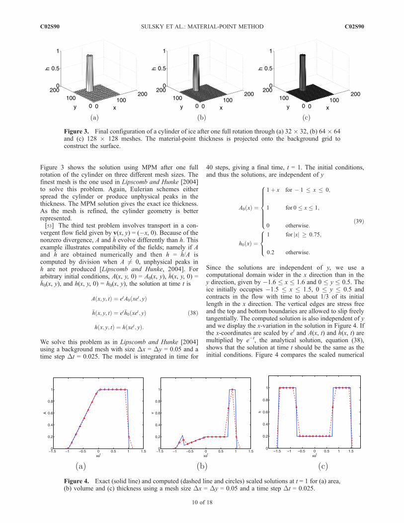
Figure 3 shows the solution using MPM after one fullrotation of the cylinder on three different mesh sizes. Thefinest mesh is the one used in Lipscomb and Hunke [2004]to solve this problem. Again, Eulerian schemes eitherspread the cylinder or produce unphysical peaks in thethickness. The MPM solution gives the exact ice thickness.As the mesh is refined, the cylinder geometry is betterrepresented.[53] The third test problem involves transport in a con-

vergent flow field given by v(x, y) = (�x, 0). Because of thenonzero divergence, A and �h evolve differently than h. Thisexample illustrates compatibility of the fields; namely if Aand �h are obtained numerically and then h = �h/A iscomputed by division when A 6¼ 0, unphysical peaks inh are not produced [Lipscomb and Hunke, 2004]. Forarbitrary initial conditions, A(x, y, 0) = A0(x, y), �h(x, y, 0) =�h0(x, y), and h(x, y, 0) = h0(x, y), the solution at time t is

A x; y; tð Þ ¼ etA0 xet; yð Þ

�h x; y; tð Þ ¼ et�h0 xet; yð Þ

h x; y; tð Þ ¼ h xet; yð Þ:

ð38Þ

We solve this problem as in Lipscomb and Hunke [2004]using a background mesh with size Dx = Dy = 0.05 and atime step Dt = 0.025. The model is integrated in time for

40 steps, giving a final time, t = 1. The initial conditions,and thus the solutions, are independent of y

A0 xð Þ ¼

1þ x for � 1 � x � 0;

1 for 0 � x � 1;

0 otherwise:

8>>>>>><>>>>>>:

h0 xð Þ ¼1 for jxj � 0:75;

0:2 otherwise:

8><>:

ð39Þ

Since the solutions are independent of y, we use acomputational domain wider in the x direction than in they direction, given by �1.6 � x � 1.6 and 0 � y � 0.5. Theice initially occupies �1.5 � x � 1.5, 0 � y � 0.5 andcontracts in the flow with time to about 1/3 of its initiallength in the x direction. The vertical edges are stress freeand the top and bottom boundaries are allowed to slip freelytangentially. The computed solution is also independent of yand we display the x-variation in the solution in Figure 4. Ifthe x-coordinates are scaled by et and A(x, t) and �h(x, t) aremultiplied by e�t, the analytical solution, equation (38),shows that the solution at time t should be the same as theinitial conditions. Figure 4 compares the scaled numerical

Figure 3. Final configuration of a cylinder of ice after one full rotation through (a) 32 � 32, (b) 64 � 64and (c) 128 � 128 meshes. The material-point thickness is projected onto the background grid toconstruct the surface.

Figure 4. Exact (solid line) and computed (dashed line and circles) scaled solutions at t = 1 for (a) area,(b) volume and (c) thickness using a mesh size Dx = Dy = 0.05 and a time step Dt = 0.025.


10 of 18

C02S90

and analytical solutions at time t = 1. Note that the linearvelocity is interpolated to the material points exactly usingthe bilinear shape functions. Also, derivatives of a linearfield are computed exactly in MPM. The time integration ofthe material-point positions and the material-point values ofA and �h should also be exact, since the equations are linear.The only errors are associated with projecting the thecomputed material-point profiles onto the background grid.The figure shows that these errors are small. Initially thereare 60 grid points of the background mesh in the x-directionand 10 in the y-direction over the ice. At time t = 1, there areonly about 16 grid points covering the ice in the x-direction.The low resolution of the final configuration is apparent,especially in the plot of �h. For comparison, the solutionis shown computed with mesh sizes Dx = Dy = 0.025 andDx = Dy = 0.0125 in Figure 5. These meshes are able toresolve the variations in �h and produce high fidelity solutions.

6.2. Wind-Driven Ice

[54] The purpose of this section is to demonstrate the fullMPM algorithm using the two constitutive models de-scribed in section 4. Schulkes et al. [1998] identify a simpletest problem that seems to distinguish properties of variousviscous and viscous-plastic ice rheologies. In that work, asimple rectangular region of ice is subjected to wind forcingand ocean drag. Two adjacent boundaries of the rectanglerepresent free surfaces and the other two boundaries repre-sent shorelines. Along the shore, the ice has no normalcomponent of velocity but is allowed to slip freely, relativeto the shore, in the tangential direction. For the MPM

Figure 5. Exact (solid line) and computed (dashed line and circles) scaled solutions at t = 1 for (a) area,(b) volume and (c) thickness using a mesh sizeDx =Dy = 0.025 and a time stepDt = 0.0125; and (d) area,(e) volume and (f) thickness using a mesh size Dx = Dy = 0.0125 and a time step Dt = 0.00625.

Figure 6. The ice is a 25 km by 50 km region discretizedusing 4 material points per element. The background gridconsists of 2.5 km square elements.


11 of 18

C02S90

calculation, a 25 km by 50 km region of ice is placed so thatthe left and bottom ice boundaries coincide with the left andbottom background-grid boundaries. The left and bottomgrid boundaries are identified with the straight shoreline.The ice is initially at rest and has a thickness of 2 m. A plotof the grid and ice region is shown in Figure 6. Thebackground grid has 2.5 km square elements The ice isdiscretized using four material points per element. Thesimulation is run for three days.[55] To begin, we compare a simulation using MPM and

the viscous-plastic rheology to the same simulation inSchulkes et al. [1998] using a finite element method. Auniform surface wind stress is applied so that ta = (0, �Ca).A linear drag relation is assumed between the base of the iceand underlying water, tw =�rwCwv, with rw representing thewater density, andCw the water drag coefficient. The velocity

v is the ice velocity and the water velocity is assumed to bezero. The initial area fraction is a uniform constant, A0 = 0.9and the initial ice thickness is h0 = 2 m. These quantitiesevolve according to equations (35) with zero thermodynamicsource terms SA = Sh = 0. Table 1 lists all of the parametersused in the simulation. The time step, Dt, is chosen fornumerical stability of an explicit update so that, for allelements, Dt < mWe/(2h), where We is the area of thecomputational element. The critical time step is about 0.01 s.[56] Figure 7 shows the computed mesh velocity in one-

day intervals. The dots in these plots represent the currentmaterial-point positions. Notice that the material pointsrepresent the geometry and a sharp edge can be maintainedeven when computations are performed on a square back-ground mesh. As expected, the ice is driven towards thebottom solid boundary and flows out, away from the shore-line along this boundary. The ice deforms substantially overthree days. The velocity and shape of the ice are quite similarto the velocity and deformed shapes shown in Schulkes et al.[1998], although it is impossible to make a quantitativecomparison because coordinates are not marked, and thevelocity scale is not given in the reference. The deformationon the third day differs slightly, but detectably, from thepublished results in Schulkes et al. [1998]. The MPM profileon day three is a bit less sloped at the top and rightboundaries, and is thus a bit wider at the top. The maximumvelocity is about 0.11 m and occurs at the lower right corner.[57] Figure 8a shows the compactness of the ice after the

first day. The ice is slightly more compact than the initialvalue of 0.9 along the bottom boundary. The largest changesin compactness occur along the upper left boundary, and thebottom right boundary. There is about a 20% reduction from0.9 to 0.7 in these regions. The upper left boundary is also aregion of divergence (Figure 8b). However, the predominantdeformation pattern is a region of shear shown in Figure 8cthat separates a low velocity region at the lower left cornerfrom a high velocity region above and to the right. Thesefields also agree with data presented by Schulkes et al.[1998].[58] The next simulation changes the rheology from

viscous-plastic to elastic-decohesvie. In line with Schreyeret al. [2006], we use the first set of material parameters

Table 1. Simulation Parameters

Name Symbol Value

Physical parametersIce density r 918 kg m�3

Air density ra 1.20 kg m�3

Air drag coefficient Ca 5 � 10�2 kg m�1 s�2

Seawater density rw 1026 kg m�3

Seawater drag coefficient Cw 5 � 10�4 m s�1

Initial conditionsInitial ice thickness h0 2 mInitial ice compactness A0 0.9

Viscous-plastic parametersIce strength parameter P* 5 � 103 kg m�1 s�2

Ice strength-compactness parameter C 15Eccentricity of ellipse e 2Viscosity cutoff zmax 2.5 � 108 s

Decohesion parameters (set 1)Young’s modulus E 1 MPaPoisson’s ratio n 0.36Failure strength in tension tnf 15.0 KPaFailure strength in shear tsf 9.0 KPaDecohesion length scale u0 100 mShear magnification factor sm 4Compressive strength f 0

c 75 KPa

Figure 7. The mesh velocity and material-point positions shown after (a) 1 day, (b) 2 days, and (c) 3 daysusing the viscous-plastic rheology.


12 of 18

C02S90

given in Table 1 for intact ice. The isotropic elasticproperties are characterized by the Young’s modulus andPoisson’s ratio, and the remaining parameters govern thedecohesion. The time stepping is explicit, with the time stepcontrolled by the CFL condition, Dt <

ffiffiffiffiffiffiWe

p/c, based on the

elastic wave speed, c ffiffiffiffiffiffiffiffiE=r

p, and the background element

area, We. For this problem, the time step is about Dt = 30 s.It is worth noting that this time step is about four orders ofmagnitude larger than the time step required for the stable,explicit viscous-plastic simulation with the same mesh size.[59] In this calculation the ice did not deform significantly

over the three days. The maximum stress in the ice is notsufficient to initiate decohesion and the ice response to

forcing is purely elastic. After a brief transient period, themotion is quasistatic and the momentum balance is primarilya balance of the wind stress and the internal forces. Anapproximate solution is obtained by assuming the ice veloc-ity is zero and the only nonzero Cauchy stress component isthe yy-component, syy. In order to balance the wind stress,syy is linear in y, zero at the top of the ice and �1250 Pa atthe bottom. The two-dimensional simulation with slipboundary conditions shows this general behavior with anapproximately linear stress profile along the y-direction, asshown in Figure 9.[60] The calculation with the viscous-plastic constitutive

model shows more flow than the elastic model. The uniaxial

Figure 8. Material-point values of (a) compactness, A, (b) divergence, r � v, and (c) shear strain rate

invariant, g, after one day, using the viscous-plastic rheology; g2 = 12tr(d̂ : d̂), d̂ = 1

2(rv + (rv)T)� 1

2(r � v)I.

The divergence and g are measured in units of 10�5 s�1.

Figure 9. Element values of the yy-component of the extra Cauchy stress using parameter set 1 fromTable 1 in the elastic-decohesive rheology.


13 of 18

C02S90

compressive strength, per unit thickness, based on thiselliptical yield curve in the viscous-plastic model is 2P* Aexp(�C(1 � A))/(1 + e2). For the parameters in Table 1, theuniaxial compressive strength is about 400 Pa, which ismuch smaller than the 75 KPa used in the elastic-decohesivemodel. In the next MPM calculation, the parameters defin-ing the failure function are reduced to more closely matchthe viscous-plastic yield surface to the decohesion surface.Specifically, tnf is reduced to 300 Pa, tsf = 180 Pa, and f 0c =1500 Pa. The other parameters are unchanged. Figure 10compares the decohesive failure function and the yieldfunction associated with the viscous-plastic model plottedin principal stress space.[61] To better resolve the large deformation, the back-

ground grid is reduced to a 1.25 km square mesh. Thecalculation is explicit in time, with the time step determinedby the CFL condition, as before. Due to the finer mesh, thetime step is about Dt = 15 s. Figures 11a–11c show the

velocity vectors after one, two and three days, respectively,for this calculation. The maximum velocity is about 0.14 mand occurs at the lower right. At the bottom boundary thereis considerable deformation of the ice as the free surfacemoves out to the right. The velocity is smaller in the lowerleft corner of the domain than elsewhere. The region oflower velocity is separated from the main flow by a zone ofhigh shear. These observations are qualitatively similar tothe results using the viscous-plastic rheology; however,details of the shape are different. The decohesive modelshows more of a dip in the top surface and more of a bulgeon the right, compared with the viscous-plastic model.Figures 12a and 12b show plots of the normal and tangentialcomponents of the displacement jump, respectively. Thesecomponents are scaled by u0 = 100 m. Thus the largestnormal opening is about 600 m and occurs near the left sideof the domain. There is also a similarly large opening alonga crack roughly normal to the right side of the ice cover. Thetangential component of the displacement jump has a largermaximum magnitude, almost 2 km. It is apparent that theshear zone seen in the velocity field corresponds to a leadwhere there is a large tangential displacement between thesides of the lead. Thus two main leads appear in thesimulation. The first lead opens and is accompanied byrelatively large shear, and the second lead mainly openswith relatively little shear. The opening of the second leaddoes not seem to correspond to any feature of the viscous-plastic simulation. The combination of fractures indicatesthat a block of ice at the lower right breaks away, and theregion just above this block falls in a shear motion relativeto the comparatively stationary ice in the lower left corner ofthe domain.

6.3. Discussion

[62] The first calculation where the ice cover remainselastic provides a simple test of the numerical method sincean approximate analytical solution can be used for compar-ison. The values of tnf, tsf and f0c used in this firstcalculation did not result in significant deformation underthe prescribed wind stress. Experiments and kinematicstudies [Schreyer et al., 2006] indicate that the parameters

Figure 10. The dashed line is a viscous-plastic yieldsurface and the solid line is a decohesive failure surface.The axes show the values of principal stresses.

Figure 11. Ice velocity after (a) 1 day, (b) 2 days, and (c) 3 days plotted on the background grid, usingthe reduced strength parameters in the elastic-decohesive rheology.


14 of 18

C02S90

used in this simulation are characteristic of an intact icecover. In contrast, there is significantly more deformationseen in computations with a viscous-plastic model shown inSchulkes et al. [1998]. In those simulations, the nominalstrength P* is low, and the initial compactness of 0.9implies that the ice cover is not intact, but contains 10%open water. The presence of water reduces the strength ofthe intact ice cover. Note that this reduction occurs uni-formly and isotropically throughout the domain.[63] The second calculation, where the decohesion

parameters are reduced, is an isotropic approximation tothe case where the ice has multiple leads throughout thatreduce its strength. This is analogous to having a lowstrength and a compactness less than one for the viscous-plastic model. Under these conditions the extent of thedeformation using the elastic-decohesive model is similarto that observed using a viscous-plastic model. Using theelastic-decohesive model, the deformation is seen to resultfrom the formation of two principal leads. One lead opensand shears while the failure mode for the second lead isprimarily an opening mode. This simulation provides anexample of the information that is available through thedecohesion model. It should be noted that once decohesioninitiates the ice is no longer an isotropic material. Thetraction on the surface of a lead goes to zero as it opens,but components of stress orthogonal to the lead can benonzero. Although not done in this paper, the area associ-ated with the open lead can be calculated. Future studies canadd thermodynamic effects that would allow the exposedwater to freeze and grow new ice. Standard methods thattrack ice thickness distributions can also be added to give amore complete model of the ice cover.[64] Instead of uniformly reducing the strength of the ice

cover when water is present, it is possible, using the elastic-decohesive model, to initialize water concentrated in leadsthat would provide directional weaknesses at various loca-tions. The ice would have material parameters associatedwith intact ice, as used in the first calculation. Using thisapproach, the weakness in the ice would no longer beisotropic and the response to wind loading would depend

on the orientation of the preexisting leads. One can imaginetwo simple cases. In the first case, preexisting leads areoriented parallel to the wind velocity, and in the second casepreexisting leads are oriented perpendicular to the windvelocity. In the first case, the parallel leads would not evolveunder the loading and the ice would have a purely elasticresponse as in the first calculation. There would be ratherlittle deformation. In the second case, the loading wouldinitially result in the leads closing, but once the leads closedan elastic response similar to that shown in the firstcalculation would occur and any significant deformationof the ice would be due to the closing leads.

7. Conclusion

[65] The material-point method has been examined formodeling sea-ice dynamics. The tests in section 6 show thatthe transport of conserved quantities and material constantscan be performed accurately and efficiently using thematerial points. The representation of ice by a collectionof unconnected Lagrangian material points also can handlethe large deformations observed in the Arctic ice pack andcan predict the location of the ice edge. MPM easily allowsthe use of any solid (or fluid) model for ice in addition to thetraditional viscous-plastic models that are normally used innumerical simulations of ice dynamics. Even models withhistory dependence, such as elastoplasticity, can beemployed. As examples, a viscous-plastic model and anelastic-decohesion model were used in this paper.[66] The newly developed elastic-decohesion constitutive

equation is a natural approach for modeling material failureand lead formation. The implementation in MPM throughthe jump in displacement as an internal variable along withweak compatibility provides a simple, efficient algorithmthat does not exhibit pathologies associated with distortedfinite elements or artificial anisotropies due to orientationeffects on the computational mesh. A simple mechanism forthe initiation of a new lead has been designed and tested aspart of this work. We also suggest an algorithm to trackthickness distributions and ice compactness that conforms

Figure 12. Material-point values of the (a) normal and (b) tangential components of the displacementjump after 3 days using the reduced strength parameters in the elastic-decohesive rheology.


15 of 18

C02S90

with the information available through the decohesionconstitutive model.[67] As has been noted in the literature, an explicit

solution of the viscous-plastic model is too costly forpractical basin-scale simulations. In practice, either animplicit method, such as Zhang and Hibler [1997], or theelastic-visccous-plastic model [Hunke, 2001] is used. In thelatter case, two-hour time steps are usual, with 120 sub-cycles on a 5 km square mesh. Thus the time intervalbetween subcycles is about 1 min. The explicit time step forthe elastic-decohesion model is roughly the same as thesubcycle time used in the elastic-viscous-plastic model forthe same mesh size. Thus the cost of the elastic-decohesionmodel is comparable to the elastic-viscous-plastic model.Overall, the elastic-decohesion model shows promise as amethod for explicitly representing leads and their effect onice motion. The solution algorithm in MPM is cost effectiveand is a plausible alternative to current basin-scale simula-tion techniques.

Appendix A: Shape Functions

[68] Shape functions are used in the MPM to interpolatebetween the background mesh and the material points, aswell as to construct approximations for the finite elementmethod on the background mesh. The background grid issubdivided into elements, We, e = 1, 2, . . ., Ne. The nodes ofthis mesh are xI(t), I = 1, . . ., Nn. If each element We has mnodes then we can refer to the nodes belonging to anindividual element with the notation xI

e(t), I = 1, . . ., m.For definiteness, consider a mesh made up of quadrilateralelements in two-dimensions with four nodes, m = 4.[69] The shape functions can be constructed through a

mapping from a master element. There are two domainsunder consideration, the master element 5 and the elementin the current configuration We(t). There is a map connectingthese two domains, the map from the master element to thecurrent configuration, x = x(x, t). Figure A1 illustrates thesedomains and map.[70] For a four-node, quadrilateral mesh, the master

element is a square and the natural coordinates are denoted

by x = (x1, x2), 0 � x1 � 1, 0 � x2 � 1. The map betweenthe master element and a finite element is

xh x; tð Þ ¼ ½xe1 1� x1ð Þ þ xe2x1� 1� x2ð Þþ ½xe4 1� x1ð Þ þ xe3x1�x2

¼ xe1 1� x1ð Þ 1� x2ð Þ þ xe2x1 1� x2ð Þþ x3x1x2 þ xe4 1� x1ð Þx2

¼X4I¼1

NeI xð ÞxeI tð Þ; on We tð Þ

ðA1Þ

where

Ne1 xð Þ ¼ 1� x1ð Þ 1� x2ð Þ Ne

2 xð Þ ¼ x1 1� x2ð Þ

Ne3 xð Þ ¼ x1x2 Ne

4 xð Þ ¼ 1� x1ð Þx2ðA2Þ

These element shape functions have the property that nodesget mapped to nodes and also, edges in the master elementget mapped to the corresponding edge in the finite element.[71] The element shape functions NI

e can be assembledinto a global shape function. For node J the shape functionsfrom the surrounding elements contribute to the globalshape function NJ, as illustrated in Figure A2. Specifically,

the formula is NJ =XNe

e¼1

X4

I¼1NIe LIJ

e , where the 4 � Nn

matrix Le is the connectivity matrix. The connectivitymatrix has zeros and ones. The IJ entry is one if elementnode number I = 1, 2, . . ., 4 corresponds to the global node,J = 1, 2, . . ., Nn, and is zero otherwise. In the figure, globalnode J corresponds to node one of element one, node two ofelement two, etc. In terms of the global shape functions, themotion is approximated by

xh x; tð Þ ¼XNn

I¼1

xI tð ÞNI xð Þ: ðA3Þ

The map xh(x, t) is one-to-one and continuous in the spatialvariable.[72] The integrals (12)–(15) are over the current con-

figuration W(t) but the shape function is defined in (A1)as a function of the master element coordinates. We must

Figure A1. Quadrilateral element with mapping from themaster element indicated.

Figure A2. The global shape function associated withnode J is assembled from shape functions defined on thesurrounding elements.


16 of 18

C02S90

view NI as a function of the current configurationthrough the composition of maps, NI(x, t) = NI(x(x, t)),where x(x, t) is the inverse of (A1). Hence, the termgrad NI(x) is computed using the chain rule, grad NI(x) =gradx NI(x)F5

�1(x, t), where F5(x, t) is the deformationgradient for the map between the master element and thecurrent configuration, F5(x, t) = @x/@x. The componentsof this deformation gradient are easy to compute over anelement from (A1), and then the 2 � 2 matrix is easilyinverted to obtain F5

�1(x, t).[73] Over a time step on a Lagrangian grid, the shape

function defined on the master element does not changewith time. This fact is significant since then a time deriv-ative of the shape function is not required in the formulasfor velocity and acceleration (8)–(9). Also, the naturalcoordinates for a material point in an element remainconstant over the Lagrangian time step. The natural coor-dinates of a material point, xp = x(xp, t), are determined byinverting (A1) at the beginning of a time step. Thesecoordinates are then used throughout the Lagrangian stepto evaluate the shape function NI(xp) = NI(x(xp, t)) = NI(xp).

[74] Acknowledgments. This material is based upon work partiallysupported by the National Science Foundation (under grant DMS-0222253), by the Minerals Management Service and the National Aero-nautics and Space Administration (under contract NNH04 CC 45C) and theOffice of Naval Research (under contract N000-14-04-M-0005).

ReferencesAnderson, D. L. (1961), Growth rate of sea ice, J. Glaciol., 3, 1170–1172.Belytschko, T., W. K. Liu, and B. Moran (2000), Nonlinear Finite Elementsfor Continua and Structures, John Wiley, Hoboken, N. J.

Bitz, C., and W. H. Lipscomb (1999), An energy-conserving thermody-namic model of sea ice, J. Geophys. Res., 104(C7), 15,669–15,677.

Brackbill, J. U., and H. M. Ruppel (1986), Flip: A method for adaptivelyzoned, particle-in-cell calculations in two dimensions, J. Comput. Phys.,65, 314.

Brackbill, J. U., D. B. Kothe, and H. M. Ruppel (1988), Flip: A low-dissipation particle-in-cell method for fluid flow, Comput. Phys. Com-mun., 48, 25–38.

Burgess, D., D. Sulsky, and J. U. Brackbill (1992), Mass matrix formulationof the FLIP particle-in-cell method, J. Comput. Phys., 103(1), 1–15.

Coon, M. (1980), A review of AIDJEX modeling, in Sea Ice Processes andModels, Proceedings of the Arctic Ice Dynamics Joint Experiment, editedby R. S. Pritchard, pp. 12–27, Univ. of Wash. Press, Seattle.

Coon, M., G. Maykut, R. Pritchard, D. Rothrock, and A. Thorndike (1974),Modeling the pack ice as an elastic-plastic material, in AIDJEX Bulletin,vol. 24, pp. 1–105, Univ. of Wash. Press, Seattle.

Coon, M. D., G. S. Knoke, D. C. Echert, and R. S. Pritchard (1998), Anoriented thickness distribution for sea ice, paper presented at 17th Int.Symp. on Ice, Int. Assoc. of Hydraul. Eng., Saint Petersburg, Russia.

Evans, M., and F. Harlow (1957), The particle-in-cell method for hydro-dynamic calculations, Tech. Rep. LA-2139, Los Alamos Sci. Lab., LosAlamos, N. M.

Flato, G. M. (1993), A particle-in-cell sea-ice model, Atmos. Ocean, 31(3),339–358.

Flato, G. M., and W. D. Hibler (1989), The effect of ice pressure onmarginal ice-zone dynamics, IEEE Trans. Geosci. Remote Sens., 27(5),514–521.

Gray, J., and L. Morland (1994), A two-dimensional model for thedynamics of sea ice, Philos. Trans. R. Soc. London A, 347, 219–290.

Gutfraind, R., and S. B. Savage (1997), Smoothed particle hydrodynamicsfor the simulation of broken-ice fields: Mohr-Coulomb-type rheology andfrictional boundary conditions, J. Comput. Phys., 134, 203–215.

Harlow, F. (1957), Hydrodyanamics problems involving large fluid distor-tions, J. Assoc. Compos. Mach., 4, 137.

Hibler, W. D. (1977a), Viscous sea ice law as a stochastic average ofplasticity, J. Res. Oceans Atmos., 82(27), 3932–3938.

Hibler, W. D. (1977b), Viscous sea ice law as a stochastic average ofplasticity, Eos Trans. AGU, 58(8), 823.

Hibler, W. D. (1979), Dynamic thermodynamic sea ice model, J. Phys.Oceanogr., 9(4), 815–846.

Hibler, W. D., and E. M. Schulson (2000), On modeling the anisotropicfailure and flow of flawed sea ice, J. Geophys. Res., 105(C7), 17,105–17,120.

Hopkins, M. A. (1998), Four stages of pressure ridging, J. Geophys. Res.,103(C10), 21,883–21,891.

Hopkins, M. A., and W. D. Hibler (1991), On the shear-strength of geo-physical scale ice rubble, Cold Reg. Sci. Technol., 19(2), 201–212.

Hopkins, M. A., W. D. Hibler, and G. M. Flato (1991), On the numerical-simulation of the sea ice ridging process, J. Geophys. Res., 96(C3),4809–4820.

Hughes, T. J. R. (2000), The Finite Element Method: Linear Static andDynamic Finite Element Analysis, Dover, Mineola, N. Y.

Hunke, E. C. (2001), Viscous-plastic sea ice dynamics with the evp model:Linearization issues, J. Comput. Phys., 170(1), 18–38.

Hunke, E. C., and J. K. Dukowicz (1997), An elastic-viscous-plastic modelfor sea ice dynamics, J. Phys. Oceanogr., 27(9), 1849–1867.

Ip, C., W. Hibler, and G. Flato (1991), On the effect of rheology on seasonalsea ice simulations, Ann. Glaciol., 15, 17–25.

Kubat, I., M. Sayed, S. Savage, and T. Carrieres (2005), Implementationand testing of a thickness redistribution model for operational ice forcast-ing, paper presented at 18th Int. Conf. on Port and Ocean Eng. UnderArctic Conditions, Clarkson, Univ., Potsdam, N. Y.

Lebedev, V. V. (1940), New formulas on the growth of ice in Arctic riversand seas, Meteorol. Gidrolog., 6(8), 40–51.

LeVeque, R. J. (1990),Numerical Methods for Conservation Laws, Springer,New York.

Lindsay, R. W., and H. L. Stern (2004), A new Lagrangian model of Arcticsea ice, J. Phys. Oceanogr., 34.

Lipscomb, W. H., and E. C. Hunke (2004), Modeling sea ice transport usingincremental remapping, Mon. Weather Rev., 132(6), 1341–1354.

Love, E., and D. L. Sulsky (2006), An unconditionally stable, energy-momentum consistent implementation of the material-point method,Comput. Methods Appl. Mech. Eng., 195, 3903–3925.

Maslowski, W., D. Marble, W. Walczowski, and A. Semtner (2001), Onlarge-scale shifts in the Arctic Ocean and sea-ice conditions during1979–98, Ann. Glaciol., 33, 545–550.

Morland, L., and R. Staroszczyk (1998), A material coordinate treatment ofsea-ice dynamics, Proc. R. Soc. London, 424, 2819–2857.

Pritchard, R. (1975), An elastic-plastic constitutive law for sea ice, J. Appl.Mech., 379–384.

Roache, P. J. (1985), Computational Fluid Dynamics, Hermosa, Albuquer-que, N. M.

Rothrock, D. A. (1975), The energetics of the plastic deformation of packice by ridging, J. Geophys. Res., 80, 4514–4519.

Savage, S. (2002), Two category sea-ice thickness redistribution model,technical report, Can. Ice Serv., Ottawa, Ont., Canada.

Sayed, M., and T. Carrieres (1999), Overview of a new operational icemodel, paper presented at Ninth Int. Offshore and Polar Eng. Conf.(ISOPE), Int. Soc. of Offshore and Polar Eng., Brest, France.

Sayed, M., T. Carrieres, H. Tran, and S. B. Savage (2002), Development ofan operational ice dynamics model for the Canadian Ice Service, paperpresented at Twelfth Int. Offshore and Polar Eng. Conf. (ISOPE), Int.Soc. of Offshore and Polar Eng., Kitakyushu, Japan.

Schreyer, H., L. Monday, D. Sulsky, M. Coon, and R. Kwok (2006),Elastic-decohesive constitutive model for sea ice, J. Geophys. Res.,111, C11S26, doi:10.1029/2005JC003334.

Schulkes, R., L. Morland, and R. Staroszczyk (1998), A finite-elementtreatment of sea ice dynamics for different ice rheologies, Int. J. Numer.Methods Geomech., 22, 153–174.

Schulson, E. M. (2001), Brittle failure of ice, Eng. Fracture Mech., 68,1839–1887.

Sulsky, D., and H. L. Schreyer (1996), Axisymmetric form of the materialpoint method with applications to upsetting and Taylor impact problems,Comput. Methods Appl. Mech. Eng., 139, 409–429.

Sulsky, D., Z. Chen, and H. L. Schreyer (1994), A particle method forhistory-dependent materials, Comput. Methods Appl. Mech. Eng., 118,179–196.

Sulsky, D., S.-J. Zhou, and H. L. Schreyer (1995), Application of a particle-in-cell method to solid mechanics, Comput. Phys. Commun., 87, 236–252.

Thorndike, A. S., and G. A. Maykut (1973), On the thickness distribution ofsea ice, AIDJEX Bull., 21, 31–48.

Thorndike, A., D. Rothrock, G. Maykut, and R. Colony (1975), The thick-ness distribution of sea ice, J. Geophys. Res., 80(33), 4501–4513.

Wang, L., and M. Ikeda (2004), A Lagrangian description of sea icedynamics using the finite element method, Ocean Modell., 7, 21–38.

Wilchensky, A., and D. Feltham (2004), A continuum anisotropic model ofsea-ice dynamics, Proc. R. Soc. London A, 460, 2105–2140.

Zhang, J. L., and W. D. Hibler (1997), On an efficient numerical method formodeling sea ice dynamics, J. Geophys. Res., 102(C4), 8691–8702.


17 of 18

C02S90

Zhang, Z. J., and S. B. Savage (1998), Particle-in-cell and finite differenceapproaches for the study of marginal ice zone problems, Cold Reg. Sci.Technol., 28, 1–28.

��M. Coon, Northwest Research Associates, Seattle, WA 98009, USA.

([email protected])

R. Kwok, Jet Propulsion Laboratory, Pasadena, CA 91109, USA.([email protected])K. Peterson and D. Sulsky, Department of Mathematics and Statistics,

University of New Mexico, Albuquerque, NM 87131, USA. ([email protected]; [email protected])H. Schreyer, Department of Engineering, University of New Mexico,

Albuquerque, NM 87131, USA. ([email protected])


18 of 18

C02S90

Using the material-point method to model sea ice dynamicssulsky/papers/SulskyEtAlJGR.pdf · Using...

Documents

Transcript of Using the material-point method to model sea ice dynamicssulsky/papers/SulskyEtAlJGR.pdf · Using...