USING THE LISP-MINER SYSTEM FORCREDIT RISK ASSESSMENT

P. Berka∗

Abstract: Credit risk assessment, credit scoring and loan applications approvalare one of the typical tasks that can be performed using machine learning or datamining techniques. From this viewpoint, loan applications evaluation is a clas-sification task, in which the final decision can be either a crisp yes/no decisionabout the loan or a numeric score expressing the financial standing of the appli-cant. The knowledge to be used is inferred from data about past decisions. Thesedata usually consist of both socio-demographic and economic characteristics of theapplicant (e.g., age, income, and deposit), the characteristics of the loan, and theloan approval decision. A number of machine learning algorithms can be used forthis purpose. In this paper we show how this task can be performed using the LISp-Miner system, a tool that is under development at the University of Economics,Prague. LISp-Miner is primarily focused on mining for various types of associationrules, but unlike “classical” association rules proposed by Agrawal, LISp-Miner in-troduces a greater variety of different types of relations between the left-hand andright-hand sides of a rule. Two other procedures that can be used for classificationtask are implemented in LISp-Miner as well. We describe the 4ft-Miner and KEXprocedures and show how they can be used to analyze data related to loan appli-cations. We also compare the results obtained using the presented algorithms withresults from standard rule-learning methods.

Key words: data mining, decision rules, association rules, credit scoring

Received: May 4, 2015 DOI: 10.14311/NNW.2016.26.029Revised and accepted: October 26, 2016

1. Introduction

Credit risk refers to the risk that a borrower will default on any type of debt byfailing to make required payments. To reduce the lender’s credit risk, the lendermay perform a credit check on the prospective borrower. The granting of creditthen depends on the confidence the lender has in the borrower’s credit worthi-ness. Most banks or lenders use some credit-scoring models (credit scorecards)to rank potential and existing customers according to their risk. One exampleis the FICO (Fair, Isaac and Company) score, the most popular credit score inthe US. The FICO score is derived from positive and negative information in the

∗Petr Berka, Dept. of Information and Knowledge Engineering, University of Economics,W. Churchill Sq. 4, CZ-130 67 Prague, Czech Republic, E-mail: berka@vse.cz

c©CTU FTS 2016 497

Neural Network World 5/2016, 497–518

credit record of a prospective borrower. This score considers the payment his-tory (e.g., bankruptcy, late payments, or foreclosures), amounts owed (various infoabout debt), length of credit history (e.g., age of accounts), new credit (e.g., typeof new credit) and types of credit used (e.g., consumer finance or mortgage). Eachparticular characteristic within every category is evaluated and added (in the formof a mathematical equation) to contribute to the final score. The five categories’proportions in the final score are: 35 % takes the payment history, 30 % takes theamounts owed, 15 % takes the length of credit history, 10% takes the new credit and10 % takes the types of credit used. The FICO score ranges from 300 to 850. Thehigher the score, the lower the risk. Another example is the Vantage score, whichevaluates the loan applicant according to six categories: payment history (this cat-egory makes up 32 % of the final score), usage of the available credit (23 %), totaldebt (15 %), past credits and credit history (13 %), number of past loan applica-tions (10 %) and amount of credits on credit cards (7 %), The Vintage score rangesfrom 501 to 990. Again, the higher the score, the better the rating. There are alsosome other scores that are used to evaluate the credit worthiness of a prospectiveloan applicant (see Tab. 1).

The main drawback of using these scores is the necessity to have availablevalues for all input variables. Without this information, the weighted sum, thatcorresponds to a score cannot be computed. It is also reported, that the FICOscore is not a good predictor in classifying between good loan applicants (whorepay their loan) and bad applicants (who do not), as the average difference ofFICO score between these two groups is very small.

Grade FICO Vantage PLUS TransUnion CreditXpert

A 750–850 901–990 740–830 845–925 800–900B 700–749 801–900 695–739 765–844 740–799C 650–699 701–800 655–694 685–764 670–739D 600–649 601–700 590–654 605–684 610–669F 300–599 501–600 300–589 150–604 300–609

Tab. I Different credit scores (credit.com).

A credit score can be used as-is, can be turned into a grade (A-F) or fuzzyconcepts (e.g., very poor, poor, fair, good, and excellent). Regardless of this rep-resentation, the final decision the bank makes is whether or not to approve a loan,i.e., to distinguish between “good” or “bad” applications. From this viewpoint,loan applications evaluation can be understood as a binary classification task. Theknowledge to be used can be inferred from data about past decisions. These datausually consist off both socio-demographic and economic characteristics of the ap-plicant (e.g., sex, income, and deposit), the characteristics of the loan, and the loanapproval decision.

A number of machine learning algorithms can be used for this purpose. In thispaper we show how this task can be solved using the LISp-Miner system, a toolthat is under development at the University of Economics, Prague. The rest of thepaper is organized as follows: Section 2 reviews related work on applying machine

498

Berka P.: Using the LISp-Miner system for credit risk assessment

learning algorithms to credit risk assessment; Section 3 presents the LISp-Minersystem; Section 4 describes the experiments carried out on data from the loanapplications domain, and Section 5 concludes the paper.

2. Related work

Credit risk assessment, credit scoring and loan applications approvals are typicaltasks that can be performed using machine learning or data mining techniques.Hence a lot of research has been carried out in this area. Chen et al. [7] use atwo-stage approach composed of k-means clustering and support vector machines(SVM) classification together with computation of feature importance. K-meansclustering is used to obtain homogeneous clusters of representative examples (iso-lated examples are eliminated, and inconsistent examples are re-labeled). The SVMclassifier is then applied to these homogeneous clusters. Vinciotti and Hand [30]compare the use of the “classical” linear approach with the k-nearest-neighbormethods. They also discuss the issue of highly imbalanced classes (usually a largemajority of applications are “good” ones) and describe four different scenarios howto handle this problem: the use of different weights for examples of different classeswhen classifying, the use of different weights for examples of different classes whenbuilding the model, the use of oversampling to balance the training data, and theuse of separability criteria based on within class score distributions. Zhou andWang [32] propose to use random forests to distinguish between good and badloans if the classes are imbalanced. They use weighted random forests (here dif-ferent weights of examples belonging to different classes are used during learning),and balanced random forests (here the data are oversampled). Lee, Chiu, Chouand Lu [20] propose to use the Classification and Regression Tree (CART) andMultivariate Adaptive Regression Splines (MARS) algorithms to classify clients ofa local bank at Taiwan. Kim and Hwang [18] integrated multi-layer perceptron,discriminant analysis and decision tree models using genetic algorithms to createa system for credit risk evaluation. Galindo and Tamayo [13] presented a com-parative analysis of different statistical and machine learning modeling methodsof classification on mortgage loan data. Kotsiantis [19] proposed a selective vot-ing method of representative machine learning algorithms (decision tree, neuralnetwork, Bayesian classifier, and k-NN classifier) to classify loan applications.

3. The LISp-Miner system

The LISp-Miner system is an academic data mining software tool developed atthe University of Economics, Prague1, which is focused on mining various rule-likepatterns from categorical data [27, 29]. The system is a successor of the GUHAmethod, an original Czech approach to association rule mining from mid-1960s[15]. Contrary to “classical” association rules, GUHA (and LISp-Miner as well)introduce a greater variety of different types of relations between the left-hand(called antecedent) and right-hand (called succedent) sides of a rule and offersmore expressive syntax for the rules.

1The system is freely available at http://lispminer.vse.cz.

499

Neural Network World 5/2016, 497–518

By now, LISp-Miner implements ten data mining procedures: 4ft-Miner (de-rived from the original GUHA procedure ASSOC), SD4ft-Miner, AC4ft-Miner, KL-Miner, CF-Miner, SDKL-Miner, SDCF-Miner, KEX, ETree-Miner and MCluster-Miner. Most of the procedures mine for various types of rule-like patterns — thismakes LISp-Miner more focused on particular type of models than standard datamining tools. The procedures 4ft-Miner, SD4ft-Miner, AC4ft-Miner, KL-Miner,CF-Miner, SDKL-Miner, and SDCF-Miner mine for patterns which are to be in-terpreted by users and domain experts. They can then be used for data description,concept description or dependency analysis tasks2, KEX and ETree-Miner can beused for classification and the procedure MC-Miner that mines for clusters of ex-amples can be used for segmentation. We will only describe in more detail the4ft-Miner and KEX procedures, as they are used in our experiments. For descrip-tion of the other procedures, see e.g., [27–29].

Most of the procedures implemented in LISp-Miner look for patterns (rules)that relate together so-called Boolean attributes. A Boolean attribute (also calleda cedent) is a conjunction of partial cedents, a partial cedent is a conjunction ordisjunction of literals and a literal is defined as A(coef) or ¬A(coef). Here A isan attribute (variable) and coef (coefficient) defines a subset of possible values ofA. So e.g., income(high), age(30-40,40-50) or ¬city(Prague,Brno,Ostrava) areexamples of literals. In these examples income(high) refers to a single value of theattribute income, age(30-40,40-50) refers to an interval created for two subsequentvalues of the discretized attribute age (numeric attributes must be discretized inadvance, prior to using LISp-Miner data mining procedures – this can be done usingthe LISp-Miner module DataSource), and ¬city(Prague,Brno,Ostrava) refers toa subset of values of the attribute city.

3.1 Association rules and the 4ft-Miner procedure

Association rules were proposed by R. Agrawal in the early 1990s as a tool forthe so-called market basket analysis [1]. An association rule has the form of animplication

X ⇒ Y, (1)

where X and Y are sets of items (itemsets) and X ∩ Y = ∅. An association ruleexpresses that transactions containing items of set X tend to contain items of setY , so e.g. a rule

{A,B} ⇒ {C} (2)

says that customers who buy products A and B also often buy product C. The twobasic characteristics of an association rule are support and confidence. Support ofan itemset X is defined as the proportion of transactions in the data set whichcontain the itemset X. Confidence of an association rule X ⇒ Y is defined assupport(X ∪ Y )/support(X). This idea of association rules can be applied to anydata in tabular, attribute-value form. So data describing values of attributes canbe analyzed in order to find associations between conjunctions of attribute-value

2Refer to the typology of data mining tasks related to the CRISP-DM methodology [6].

500

Berka P.: Using the LISp-Miner system for credit risk assessment

Cond Suc ¬Suc∑

Ant a b r¬Ant c d s∑

k l n

Tab. II Four-fold contingency table created for examples satisfying condition γ.

pairs (categories). Let us denote these conjunctions as Ant (antecedent) and Suc(succedent) and the association rule as

Ant⇒ Suc. (3)

When using association rules for concept description, Suc will be a category of thetarget attribute.

The 4ft-Miner procedure3 offers a more general form of the above-describedassociation rules. 4ft-Miner mines for patterns (4ft-rules) of the form

Ant ≈ Suc/Cond, (4)

where Ant, Suc and Cond (condition) are cedents, and ≈ (called quantifier) denotesa relationship between Ant and Suc for the examples from the analyzed data tablethat fulfill Cond. If the condition is empty then the procedure analyzes the wholedata table. The relationships between Ant and Suc are defined (and evaluated)using frequencies from the four-fold contingency table as shown in Tab. 3.1; here adenotes the number of examples that fulfill both Ant and Suc, b denotes the numberof examples that fulfill Ant but not Suc, c denotes the number of examples thatfulfill Suc but not Ant, and d denotes the number of examples that fulfill neitherAnt nor Suc. We sometimes use r = a + b, k = a + c, s = c + d, l = b + d andn = a+ b+ c+ d.

Examples of relationships between Ant and Suc as defined for the frequenciesfor the four-fold table, are a founded implication ⇒ defined as

a

a+ b, (5)

a founded equivalence = defined as

a+ b

a+ b+ c+ d, (6)

or an χ2 chi-squared quantifier defined as

(ad− bc)2

rklsn. (7)

The 4ft-Miner procedure contains almost 20 different types of those relationships.Their description can be found e.g. in [27].

3This procedure extends the original GUHA procedure ASSOC from the mid. 1960s. Theauthors of 4ft-Miner as well as of most of the other procedures are Jan Rauch and Milan Simunek.

501

Neural Network World 5/2016, 497–518

Let us assume a toy loan application domain consisting of attributes income(having values low and high), balance (having values low, medium, and high), sex(having values male and female), unemployed (having values yes and no), and loan(having values yes and no). An example of a 4ft-rule can be

balance(high,medium) ∧ ¬unemployed(yes)⇒ loan(yes)/sex(male) (8)

which says that in the group of men, if a person has a high or medium balance onhis account and is not unemployed, then he will get the loan. 4ft-rules are thusmuch more expressive than “standard” association rules, where the only possibleexample is of the following type:

income(high) ∧ balance(high)⇒ loan(yes). (9)

When running an 4ft task, the user should specify the literals that can be usedto compose Ant, Suc, and Cond, and the type and parameters that define therelation between Ant and Suc (e.g., formulas (5), (6), (7) with lower bounds ontheir values), and the lower bound for frequency a from the four-fold contingencytable.

Unlike the well-known apriori algorithm, where single itemsets (i.e., conjunc-tions of categories) are generated in the first step and then each itemset (con-junction) is divided into antecedent and succedent [1], in 4ft-Miner each part of arule (i.e., antecedent, succedent, and eventually condition) is generated separately,so we can easily set the target attribute as the only one that can occur in thesuccedents. Moreover, we can control the complexity of the searched rule space bydetermining (using parameters maxlenA, maxlenS and maxlenC) the maximumnumber of literals that can occur in cedents of each respective part of a rule.

The result of the analysis using 4ft-Miner is usually a huge set of rules thatshould be inspected and evaluated by the domain experts and users (see Fig. 2).Let us stress here that the quantitative characteristics of the found rules do notguarantee usefulness of the rules. We can find a lot of rules with high confidence(especially those with low support), that do not represent any reasonable knowl-edge.

3.2 Decision rules and the KEX procedure

Decision rule in the form

Ant⇒ C, (10)

where Ant (antecedent, condition) is a conjunction of values of input attributes(called categories or selectors) and C is a category of class attribute C, are one ofthe most popular formalisms of how to express classification models learned fromdata. The commonly used approach to learning decision rules is the set coveringapproach also called “separate and conquer”. The basic idea of this approach isto create a rule that covers some examples of a given class, and remove theseexamples from the training set (see Algorithm 1). This is repeated for all examplesnot covered so far. The other way to create decision rules is the compositionalapproach. In this approach the covered examples are not removed during learning,

502

Berka P.: Using the LISp-Miner system for credit risk assessment

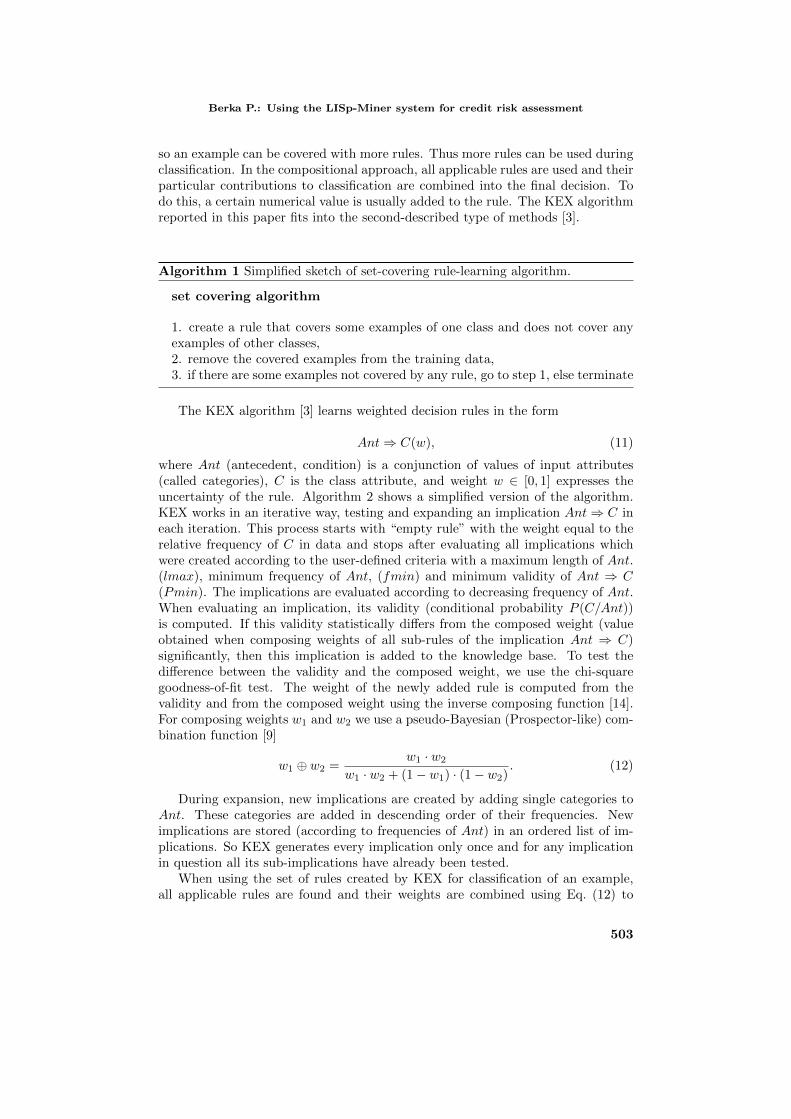
so an example can be covered with more rules. Thus more rules can be used duringclassification. In the compositional approach, all applicable rules are used and theirparticular contributions to classification are combined into the final decision. Todo this, a certain numerical value is usually added to the rule. The KEX algorithmreported in this paper fits into the second-described type of methods [3].

Algorithm 1 Simplified sketch of set-covering rule-learning algorithm.

set covering algorithm

1. create a rule that covers some examples of one class and does not cover anyexamples of other classes,2. remove the covered examples from the training data,3. if there are some examples not covered by any rule, go to step 1, else terminate

The KEX algorithm [3] learns weighted decision rules in the form

Ant⇒ C(w), (11)

where Ant (antecedent, condition) is a conjunction of values of input attributes(called categories), C is the class attribute, and weight w ∈ [0, 1] expresses theuncertainty of the rule. Algorithm 2 shows a simplified version of the algorithm.KEX works in an iterative way, testing and expanding an implication Ant⇒ C ineach iteration. This process starts with “empty rule” with the weight equal to therelative frequency of C in data and stops after evaluating all implications whichwere created according to the user-defined criteria with a maximum length of Ant.(lmax), minimum frequency of Ant, (fmin) and minimum validity of Ant ⇒ C(Pmin). The implications are evaluated according to decreasing frequency of Ant.When evaluating an implication, its validity (conditional probability P (C/Ant))is computed. If this validity statistically differs from the composed weight (valueobtained when composing weights of all sub-rules of the implication Ant ⇒ C)significantly, then this implication is added to the knowledge base. To test thedifference between the validity and the composed weight, we use the chi-squaregoodness-of-fit test. The weight of the newly added rule is computed from thevalidity and from the composed weight using the inverse composing function [14].For composing weights w1 and w2 we use a pseudo-Bayesian (Prospector-like) com-bination function [9]

w1 ⊕ w2 =w1 · w2

w1 · w2 + (1− w1) · (1− w2). (12)

During expansion, new implications are created by adding single categories toAnt. These categories are added in descending order of their frequencies. Newimplications are stored (according to frequencies of Ant) in an ordered list of im-plications. So KEX generates every implication only once and for any implicationin question all its sub-implications have already been tested.

When using the set of rules created by KEX for classification of an example,all applicable rules are found and their weights are combined using Eq. (12) to

503

Neural Network World 5/2016, 497–518

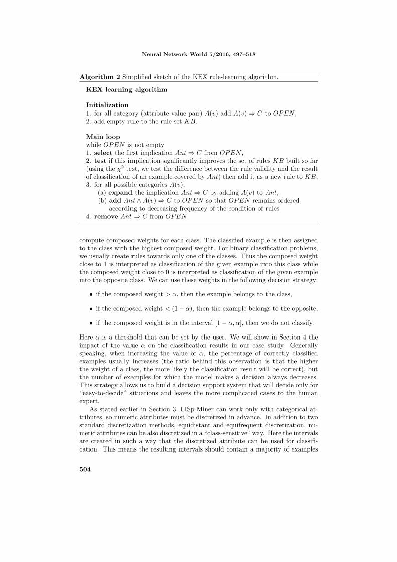
Algorithm 2 Simplified sketch of the KEX rule-learning algorithm.

KEX learning algorithm

Initialization1. for all category (attribute-value pair) A(v) add A(v)⇒ C to OPEN ,2. add empty rule to the rule set KB.

Main loopwhile OPEN is not empty1. select the first implication Ant⇒ C from OPEN ,2. test if this implication significantly improves the set of rules KB built so far(using the χ2 test, we test the difference between the rule validity and the resultof classification of an example covered by Ant) then add it as a new rule to KB,3. for all possible categories A(v),

(a) expand the implication Ant⇒ C by adding A(v) to Ant,(b) add Ant ∧A(v)⇒ C to OPEN so that OPEN remains ordered

according to decreasing frequency of the condition of rules4. remove Ant⇒ C from OPEN .

compute composed weights for each class. The classified example is then assignedto the class with the highest composed weight. For binary classification problems,we usually create rules towards only one of the classes. Thus the composed weightclose to 1 is interpreted as classification of the given example into this class whilethe composed weight close to 0 is interpreted as classification of the given exampleinto the opposite class. We can use these weights in the following decision strategy:

• if the composed weight > α, then the example belongs to the class,

• if the composed weight < (1−α), then the example belongs to the opposite,

• if the composed weight is in the interval [1− α, α], then we do not classify.

Here α is a threshold that can be set by the user. We will show in Section 4 theimpact of the value α on the classification results in our case study. Generallyspeaking, when increasing the value of α, the percentage of correctly classifiedexamples usually increases (the ratio behind this observation is that the higherthe weight of a class, the more likely the classification result will be correct), butthe number of examples for which the model makes a decision always decreases.This strategy allows us to build a decision support system that will decide only for“easy-to-decide” situations and leaves the more complicated cases to the humanexpert.

As stated earlier in Section 3, LISp-Miner can work only with categorical at-tributes, so numeric attributes must be discretized in advance. In addition to twostandard discretization methods, equidistant and equifrequent discretization, nu-meric attributes can be also discretized in a “class-sensitive” way. Here the intervalsare created in such a way that the discretized attribute can be used for classifi-cation. This means the resulting intervals should contain a majority of examples

504

Berka P.: Using the LISp-Miner system for credit risk assessment

belonging to one class. There is a number of such class-sensitive discretization algo-rithms [10,17,21]. In our experiments reported in Section 4 we used a discretizationalgorithm closely related to KEX [4]. Algorithm 3 shows a simplified sketch of thisalgorithm. The algorithm starts by creating initial intervals for each value of thenumeric attribute that occurs in the data and then merges the neighboring inter-vals if they share the same qualitative distribution of examples into classes (i.e.,they share the same majority class).

Algorithm 3 Discretization for KEX.

KEX discretization algorithm

Initialization1. For each value of the attribute create an initial interval Int and assign it toa majority class if such a class exists, otherwise label it as “UNKNOWN”.

Main loop1. Merge intervals with the same class label.2. Resolve ambiguities (if an interval Inti is labeled as “UNKNOWN”, merge itwith the previous interval Inti−1 or the following interval Inti+1).

4. Experiments with the loan application data

We used the 4ft-Miner and KEX procedures to analyze several data sets from thecredit risk assessment domain. The first three data sets are taken from the UCIMachine Learning Repository that contains a number of reference data sets usedby the machine learning community to evaluate various machine learning and datamining algorithms (www.ics.uci.edu/~mlearn/MLRepository.html). Australiancredit data is used for credit card applications. The dataset contains a mixtureof continuous, nominal with small numbers of values, and nominal with largernumbers of values attributes. All attribute names and values have been changedto meaningless symbols to protect confidentiality of the data. This data set wasfirst used by Quinlan in 1987 [23]. German credit data were provided by prof.Hofmann from the University of Hamburg; this data consists of 7 numerical and13 categorical input attributes. Japan Credit Data set represents consumer loansfor a specific purpose (e.g., car, or a PC); this data set was prepared by ChiharuSano in 1992. The Discovery Challenge data set was prepared for the DiscoveryChallenge workshop held at the European Conference of Principles and Practice onKnowledge Discovery PKDD1999 [2], the analyzed table (6181 examples, 7 inputattributes) is an excerpt from the whole database used in the workshop.

Tab. III shows the basic characteristics of the used data (number of examples,number of attributes, number of classes, and the default accuracy computed as thepercentage of the majority class). The last column, maximal accuracy, reflects the

505

Neural Network World 5/2016, 497–518

Data examples attributes classes default acc. maximal acc.

ACred 690 15 2 0.56 0.99GCred 1000 20 2 0.70 1.00JCred 125 10 2 0.68 1.00DChall 6181 7 2 0.88 1.00

Tab. III Basic characteristics of the used data sets.

amount of noise in the data4. Some data sets contain only categorical attributes;these data sets can be used directly without pre-processing. Other data sets containnumeric attributes. In this case, the data must be discretized prior to the use ofthe learning algorithms.

In our experiments we compared the results obtained with the two proceduresdescribed in the previous subsections (4ft-Miner and KEX) with the results ob-tained when using standard rule-learning algorithms as implemented in Weka, awell-known free data mining suite from University Waikato, New Zealand [16].

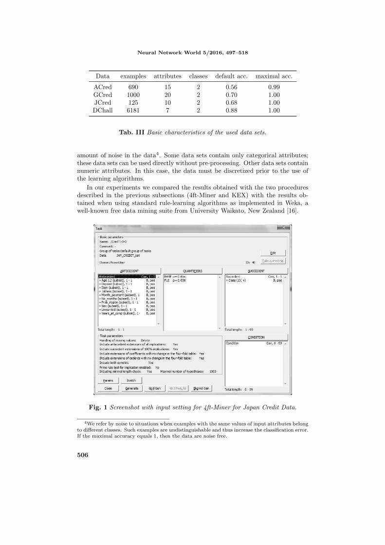
Fig. 1 Screenshot with input setting for 4ft-Miner for Japan Credit Data.

4We refer by noise to situations when examples with the same values of input attributes belongto different classes. Such examples are undistinguishable and thus increase the classification error.If the maximal accuracy equals 1, then the data are noise free.

506

Berka P.: Using the LISp-Miner system for credit risk assessment

In the first experiment, we applied 4ft-Miner to find strong interesting relation-ships between input attributes and class; we can view such relationships as conceptdescriptions of the respective classes. While strong relations can be found auto-matically (in our experiment by setting the founded implication p = 0.9), what isinteresting should be determined by the domain expert. The screenshot in Fig. 1shows the input settings of this experiment for Japan Credit Data and the screen-shot in Fig. 2 shows the corresponding results. Tab. 4 shows some of the strongrules found in the Japan Credit Data. Here high confidence and high support iden-tifies a (relatively) large group of good loan applicants, in our case men and/orolder persons working for the same company for several years (rules 7 and 10).

Fig. 2 Screenshot with example results of 4ft-Miner for Japan Credit Data.

no. Hypothesis Conf Supp

01: Age(c) & Month payment(c) ⇒ Class(+) 1.00 0.0902: Item(j) & Years at comp(b) ⇒ Class(+) 1.00 0.1403: Jobless(n) & Month payment(c) ⇒ Class(+) 1.00 0.1304: Month payment(c) & No months(b) ⇒ Class(+) 1.00 0.1005: Month payment(c) & Unmarried(n) ⇒ Class(+) 1.00 0.0906: Month payment(c) & Years at comp(b) ⇒ Class(+) 1.00 0.0907: Sex(m) & Years at comp(b) ⇒ Class(+) 0.97 0.2708: Unmarried(y) & Years at comp(b) ⇒ Class(+) 0.96 0.1809: Deposit(f) & Years at comp(b) ⇒ Class(+) 0.95 0.1610: Age(c) & Years at comp(b) ⇒ Class(+) 0.95 0.30

Tab. IV Strong association rules found by 4ft-Miner for Japan Credit Data.

We also compared between 4ft-Miner and KEX. The idea of this comparisonwas to have a look at the “reduction rate” that KEX applies to the implications(association rules) when deciding if an implication should be added to the KB or

507

Neural Network World 5/2016, 497–518

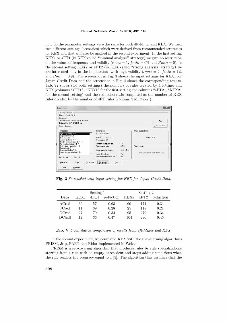
not. So the parameter settings were the same for both 4ft-Miner and KEX. We usedtwo different settings (scenarios) which were derived from recommended strategiesfor KEX and that will also be applied in the second experiment. In the first settingKEX1 or 4FT1 (in KEX called “minimal analysis” strategy) we give no restrictionon the values of frequency and validity (lmax = 1, fmin = 0% and Pmin = 0), inthe second setting KEX2 or 4FT2 (in KEX called “strong analysis” strategy) weare interested only in the implications with high validity (lmax = 2, fmin = 1%and Pmin = 0.9). The screenshot in Fig. 3 shows the input settings for KEX1 forJapan Credit Data and the screenshot in Fig. 4 shows the corresponding results.Tab. ?? shows (for both settings) the numbers of rules created by 4ft-Miner andKEX (columns “4FT1”, “KEX1” for the first setting and columns “4FT2”, “KEX2”for the second setting) and the reduction ratio computed as the number of KEXrules divided by the number of 4FT rules (column “reduction”).

Fig. 3 Screenshot with input setting for KEX for Japan Credit Data.

Setting 1 Setting 2Data KEX1 4FT1 reduction KEX2 4FT2 reduction

ACred 36 57 0.63 60 174 0.34JCred 11 39 0.28 25 118 0.21GCred 27 79 0.34 95 279 0.34DChall 17 36 0.47 104 230 0.45

Tab. V Quantitative comparison of results from 4ft-Miner and KEX.

In the second experiment, we compared KEX with the rule-learning algorithmsPRISM, Jrip, PART and Ridor implemented in Weka.

PRISM is a set-covering algorithm that produces rules by rule specializationsstarting from a rule with an empty antecedent and stops adding conditions whenthe rule reaches the accuracy equal to 1 [5]. The algorithm thus assumes that the

508

Berka P.: Using the LISp-Miner system for credit risk assessment

Fig. 4 Screenshot with example results of KEX for Japan Credit Data.

data are noise-free. PRISM was inspired by the decision tree learning algorithmID3 [22]. But unlike ID3, where the best splitting attribute is found, the bestattribute-value pair (category) is identified in PRISM. To do this, the informationgain is computed using

I(A(v), C) = log2

(P (C|A(v))

P (C)

)(13)

and the category A(v) with the highest information gain is selected5.As P (C) is constant for different A(v) and binary logarithm is an increasing

function, it is sufficient to select the best category by maximizing P (C|A(v)). The“create a single rule” part of the generic set-covering algorithm shown in Algo-rithm 1 thus has the form shown in Algorithm 4.

Jrip is an implementation of the RIPPER (Repeated Incremental Pruning toProduce Error Reduction) algorithm. This algorithm is again a variant of the set-covering approach. It performs rule induction (top-down specialization of rules)followed by a post-processing step that prunes the rules to improve the classificationaccuracy [8]. The algorithm was intended to learn rules from large noisy data. Jriprepeatedly creates a rule on a growing set and prunes it on a pruning set. A ruleis created in a top-down manner, adding a category A(v) or a condition A ≤ θor A ≥ θ (Jrip can thus directly work with numeric attributes). The best rulespecialization is selected by maximizing the information gain adopted from the ILPrule-learning system FOIL [24]. The “create a single rule” part of the algorithm isshown in Algorithm 5.

5We use the same notation as in our description of KEX in Section 3.2.

509

Neural Network World 5/2016, 497–518

Algorithm 4 Prism one rule generating algorithm.

Generate one rule

1. for a given (sub)set of examples, find a category with the highest informationgain and add this category A(v) to the antecedent of the rule,2. select for further rule specialization a subset of examples that corresponds tocategory A(v),3. if the rule does not cover only examples of the class C go to step 1, elseterminate.

Algorithm 5 Simplified sketch of Jrip rule-generating part.

Generate one rule

split uncovered examples into a growing set and a pruning set on growing set do

1. add A(v) or A ≤ θ or A ≥ θ that maximizes the information gain to the Antof the rule,2. if rule covers some negative examples, go to step 1, else terminate,

on pruning set do

3. remove a final sequence of conditions from Ant to maximize the ratio (p −n)/(p + n), where p denotes the number positive examples of the class coveredby the rule and n is the number of negative examples of the class covered by therule.

PART is a set-covering algorithm based on partial decision trees. To make asingle rule, a pruned decision tree is built for the current (sub)set of examples andthe path to the leaf with the largest coverage is turned into a rule [11]. To reducethe computational time of the algorithm (a naive implementation will create andprune a full tree for every rule), partial decision trees are created during the rulecreation process instead. A partial decision tree is a tree that contains branchesto undefined subtrees, i.e. contain nodes that were not expanded. Algorithm 6shows the algorithm for creating partial trees. The way how a splitting attribute isselected and how the tree is pruned is the same as used in the C4.5 algorithm [25].

Algorithm 6 Simplified sketch of partial tree-generating algorithm.

partial tree algorithm

choose splitting attribute of given set of examples into subsetswhile there are subsets that have not been expanded and all the subsets ex-panded so far are leaves

choose next subset to be expanded and expand itif all subsets expanded are leaves try to replace node by leaf

510

Berka P.: Using the LISp-Miner system for credit risk assessment

The Ridor (RIpple DOwn Rules) algorithm learns rules in noisy domains, i.e.,rules that need not to have 100% classification accuracy. This algorithm recursivelygenerates (by rule specialization) if-true and if-false rules [12]. The ripple downrules form a binary tree, where each node corresponds to an antecedent and thebranches correspond to true/false values. If a parent rule is activated (i.e., itsantecedent is true) then its child if-true rule is checked. If the child if-true ruleis activated, then the class assigned to the example will correspond to the classof this rule; otherwise the class assigned to the example will correspond to theclass of the parent rule. If the parent rule is not activated, its if-false child ruleis checked. If the child if-false rule is activated, then the class assigned to theexample will correspond to the class of this rule. The algorithm for generating asingle rule is inspired by the PRISM algorithm [5], but the stopping condition forrule specialization is different. Algorithm 7 shows its steps, a formula

r =

s∑i=c

(s

i

)pi(1− p)s−i (14)

is used to assess the quality of a category or of a rule (r should be maximized).Here p stands for the relative frequency of the class, s stands for the number ofexamples covered by the category or rule, and c stands for the number of examplesthat are covered and belong to the class. To create the ripple-down structure, thisalgorithm is recursively called twice. The if-true child rule is created for the nextmost frequent class of the examples covered by the parent rule. The if-false childrule is created for the same class as the parent rule but the computation is carriedout for the examples not covered by the parent rule.

Algorithm 7 Ridor one rule-generating algorithm.

Generate one rule

1. select the most frequent class as the current class,2. for given (sub)set of examples find the best category A(v),3. if adding the best category A(v) will improve the quality of the rule, then addthis category to the rule and go to step 2, else terminate,

Tab. VI summarizes the achieved results. The table shows for each of the usedlearning algorithms the number of rules and the classification accuracy reachedusing a 10-fold cross-validation test. We used standard settings for PRISM, Jrip,PART and Ridor and two different settings for KEX. Here, KEX1 and KEX2 aredefined in the same way as when comparing KEX and 4ft-Miner. Numbers in boldprint denote for each data set the best results in terms of classification accuracyand size of the rule set. We compute an overall rank as a weighted sum

2× acc.rank + rul.rank. (15)

The “winning” algorithm is the algorithm that minimizes this sum. So, e.g., forJapan Credit Data, KEX2 was the best in accuracy and fifth in rule-set size (whichgives the overall rank of 2 × 1 + 5 = 7), and PRISM was third in accuracy and

511

Neural Network World 5/2016, 497–518

first in rule set size (which gives the overall rank 2× 3 + 1 = 7); 7 was the smallestvalue of the overall rank achieved for this data. The table suggests that PARTwas outperformed by the other algorithms (PART never became a winner), andthat the other algorithms are comparable. But no general conclusions about thesuperiority of an algorithm can be drawn from the experiments. Actually, thewell-known no-free-lunch theorem gives an evidence that there is no single “best”machine learning algorithm regardless on the analyzed data [31].

Data KEX1 KEX2 PART PRISM Jrip Ridorrul./acc. rul./acc. rul./acc. rul./acc. rul./acc. rul./acc.

ACred 36/0.86 60/0.83 29/0.85 197/0.76 5/0.85 6/0.85JCred 11/0.76 25/0.79 7/0.72 4/0.74 5/0.71 4/0.70GCred 27/0.73 95/0.71 68/0.70 362/0.66 8/0.69 2/0.71DChall 17/0.88 104/0.88 134/0.98 203/0.99 41/0.96 73/0.92

Tab. VI Classification results of KEX and other rule learning algorithms.

The results shown in Tab. VI present the classification accuracy of KEX forthe value of the threshold α set to 0.5. For this setting, all examples for which thecomposed weight of the class differs from 0.5 will be classified. Figs. 5 - 8 showthe effect of different values of α on the classification accuracy and the ratio ofclassified examples (out of all examples). In all graphs the x-axis gives the valuesof α, and the y-axis gives the classification accuracy or the number of classifiedexamples respectively. The graphs in Figs. 5 and 6 show the results for the “minimalanalysis” strategy and graphs in Figs. 7 and 8 show the results for the “stronganalysis” strategy. We can conclude from these graphs that

• as we expected, when increasing the value of α, the classification accuracy(i.e., the relative number of correctly classified examples out of all classifiedexamples) increases and the relative number of classified examples (out of allexamples) decreases;

• when increasing the value of α, the improvement of classification accuracywas slightly better for the minimal analysis strategy, but at the same timethe decrease of the number of classified examples for the minimal analysisstrategy was significantly higher. This seems to indicate that the results forstrong analysis are more robust.

We present the source of the difference between the results of KEX1 and KEX2settings for Japan Credit Data in Figs. 9 and 10. Both graphs have the classindicator values on the x-axis (to be able to better display the graph we jitter thevalues of class 1 in the range 0.8 to 1.2 and the values of class −1 in a range from−1.2 to −0.8) and the composed weight on the y-axis.

A perfect rule base created by KEX would assign weights greater than 0.5 toexamples of class 1 and weights smaller than 0.5 to examples of class −1. Socorrectly classified examples are (in both Figures) indicated by the rectangles.Since the composed weights are closer to the extreme values 0 and 1 for the KEX2

512

Berka P.: Using the LISp-Miner system for credit risk assessment

Fig. 5 The impact of α on the classification accuracy, KEX1 setting.

Fig. 6 The impact of α on the number of classified examples, KEX1 setting.

setting, when increasing the value of α we will be able to classify more examplesthan for the KEX1 setting. We can also see that when using the KEX2 setting, noexample of class 1 was misclassified as an example of class −1.

513

Neural Network World 5/2016, 497–518

Fig. 7 The impact of α on the classification accuracy, KEX2 setting.

Fig. 8 The impact of α on the number of classified examples, KEX2 setting.

514

Berka P.: Using the LISp-Miner system for credit risk assessment

Fig. 9 Composed weights assigned to examples, KEX1 setting.

Fig. 10 Composed weights assigned to examples, KEX2 setting.

5. Conclusions

Credit risk assessment, credit scoring or loan applications approval are typical tasksthat can be performed using machine learning or data mining techniques. Fromthis viewpoint, loan applications evaluation is a classification or concept-descriptiontask, in which the learned knowledge is inferred from data about past decisions.

515

Neural Network World 5/2016, 497–518

Rule-learning algorithms are easier for humans to understand, when compared,e.g., with regression models, neural networks or SVM-created models.

This paper presents two data mining procedures implemented in the LISp-Minersystem (4ft-Miner and KEX) and shows how these procedures can be used for thecredit risk assessment task. 4ft-Miner is primary intended for association rulesmining. Because each part of the rule is generated separately, 4ft-Miner can easilybe used for concept description; here the succedent remains unchanged and mustbe set to the category defining the concept. KEX creates a set of rules that can beused directly for classification.

Our aim was to check the feasibility of both procedures for the given taskby comparing them with the state-of-the-art rule-learning algorithms. We choosethe PRISM, Jrip, PART and Ridor algorithms implemented in the Weka datamining system for this comparison. The empirical comparison is based on fourdata sets from the loan application domain. The results of experiments reportedin Section 4 show that there is no single best algorithm that would outperformthe other algorithms. KEX, PRISM, Jrip and Ridor each became the winningalgorithm at least once when using the criterion based on the weighted sum ofranks achieved for accuracy and size of the rule set. 4ft-Miner cannot be used inthis comparison as the resulting rules are not directly used for classification. Wecan thus compare the result of 4ft-Miner with the other algorithms only in terms ofthe size of the rule set. Here we can see from Tab. V and Tab. VI that 4ft-Minerusually creates more rules than the other algorithms. 4ft-Miner thus describes theconcept in more ways and helps to gain broader insight into the knowledge hiddenin the data.

We can also compare the algorithms themselves on the basis of their analysis.Here we can see that PART, PRISM, Jrip and Ridor all follow the set coveringprinciple. That is, examples covered by a rule are removed from the trainingdata. The consequence of this principle is that just one rule is applicable whenclassifying an example. This makes the classification process very simple (scan therule set to find an applicable rule), but narrows the way the class is described.On the contrary, 4ft-Miner and KEX, repeatedly go through the whole trainingset when creating the rules. This results in the fact, that more rules can cover anexample. For 4ft-Miner it means that partially overlapping rules can be obtained(as illustrated on the rules 07 and 10 in Tab. 4). The consequence for KEX is in thenecessity to consider a higher number of applicable rules during classification. Thesolution for this problem is described in Section 3.2; KEX uses a compositionalapproach inspired by uncertainty processing in early expert systems. Anotherdifference between KEX and the other rule-learning algorithms is that KEX doesnot perform crisp yes/no classification but assigns weights to the classes. This,together with the possibility to tune resulting decision strategy (in our case thefinal loan approval decision based on the classification result by setting the valueof parameter α) brings an extra advantage over a simple yes/no decision.

To summarize the results of the evaluation and comparison, 4ft-Miner is wellsuited for the concept description task offering alternative viewpoints on identicalexamples belonging to the target concept and KEX is well suited for creatingdecision support systems that do not take over too much responsibility from thehuman users (which can be a crucial requirement in the loan application domain).

516

Berka P.: Using the LISp-Miner system for credit risk assessment

Acknowledgement

This paper was prepared with the contribution of long-term institutional supportof research activities by the Faculty of Informatics and Statistics, University ofEconomics, Prague.

References

[1] AGRAWAL R., IMIELINSKI T., SAWAMI A. Mining associations between sets of itemsin massive databases. In: Proc. of the ACM-SIGMOD Int. Conference on Management ofData, Washington D.C. 1993, pp. 207–216, doi: 10.1145/170036.170072.

[2] BERKA P. Workshop Notes on Discovery Challenge, Prague, Univ. of Economics, 1999.

[3] BERKA P. Learning compositional decision rules using the KEX algorithm. Intelligent DataAnalysis. 2012, 16(4), pp. 665–681, doi: 10.3233/IDA-2012-0543.

[4] BRUHA I., BERKA P. Empirical Comparison of Various Discretization Procedures. Int.J.of Pattern recognition and Artificial Intelligence. 1998, 12(7), pp. 1017–1032, doi: 10.1142/S0218001498000567.

[5] CENDROWSKA J. PRISM: An algorithm for inducing modular rules. Int. J. of Man-Machine Studies. 1987, 27(4), pp. 349–370, doi: 10.1016/s0020-7373(87)80003-2.

[6] CHAPMAN P., CLINTON J., KERBER R., KHABAZA T., REINARTZ T. SHEARER C.,WIRTH R. CRISP-DM 1.0 Step-by-step data mining guide. 2000, SPSS Inc.

[7] CHEN W., XIANG G., LIU Y., WANG K. Credit risk Evaluation by hybrid data miningtechnique. Systems Engineering Procedia. 2012, 3, pp. 194–200, doi: 10.1016/j.sepro.2011.10.029.

[8] COHEN W. Fast Effective Rule Induction. In: 12th International Conference on MachineLearning, Tahoe City, California. 1995, pp. 115–123, doi: 10.1016/b978-1-55860-377-6.

50023-2.

[9] DUDA R.O., GASCHING J.E., HART P. Model Design in the Prospector Consultant Systemfor Mineral Exploration. In: WEBER, NILSSON ed., Readings in Artificial Intelligence.Elsevier, 1981, doi: 10.1016/B978-0-934613-03-3.50028-3.

[10] FAYYAD U., IRANI K. Multi-interval discretization of continuous-valued attributes for clas-sification learning, In: Proc. 13th Joint Conf. of Artificial Intelligence (IJCAI’93), 1993, pp.1022–1027.

[11] FRANK E., WITTEN I.H. Generating Accurate Rule Sets Without Global Optimization,In: Fifteenth International Conference on Machine Learning. 1998, pp. 144–151.

[12] GAINES B.R., COMPTON P. Induction of Ripple-Down Rules Applied to Modeling LargeDatabases. J. Intell. Inf. Syst. 1995, 5(3), pp. 211–228, doi: 10.1007/BF00962234.

[13] GALINDO J., TAMAYO P. Credit Risk Assessment using Statistical and Machine Learning:Basic Methodology and Risk Modeling Applications. Computational Economics. 2000, 15(1-2), pp. 107–143.

[14] HAJEK P. Combining Functions for Certainty Factors in Consulting Systems. Int. J. Man-Machine Studies. 1985, 22, pp. 59–76, doi: 10.1016/S0020-7373(85)80077-8.

[15] HAJEK P., HAVRANEK T. Mechanising Hypothesis Formation - Mathematical Foundationsfor a General Theory. Springer, 1978, doi: 10.1007/978-3-642-66943-9.

[16] HALL M., FRANK E., HOLMES H., PFAHRINGER B., REUTWMANN P., WITTENI. The WEKA Data Mining Software: An Update. SIGKDD Explorations. 2009, 11(1),doi: 10.1145/1656274.1656278.

[17] KERBER R. ChiMerge: Discretization of Numeric Attributes. In: Proc. AAAI-92 confer-ence. AAAI Press, 1992, pp. 123–128.

[18] KIM K.S., HWANG H.J. An Integrated Data Mining Model for Customer Credit Evalua-tion. In: Proc. Int. Conf. Computational Science and Its Applications ICCSA, Singapore.Springer, 2005, s.vol. 3482, pp. 798–805, doi: 10.1007/11424857_87.

517

Neural Network World 5/2016, 497–518

[19] KOTSIANTIS S. Credit risk analysis using a hybrid data mining model. Int. J. IntelligentSystems Technologies and Applications. 2007, 2(4), pp. 345–356, doi: 10.1504/ijista.2007.014030.

[20] LEE T.S., CHIU CH., CHOU Y.CH., LU CH. Mining the customer credit using classificationand regression tree and multivariate adaptive regression splines. Computational Statistics &Data Analysis. 2006, 50(4), pp. 1113–1130, doi: 10.1016/j.csda.2004.11.006.

[21] LEE C., SHIN D. A context-sensitive discretization of numeric attributes for classificationlearning. In: COHN ed., 11th European Conf. on Artificial Intelligence (ECAI’94). JohnWiley, 1994, pp. 428–432.

[22] QUINLAN J.R. Induction of decision trees. Machine Learning. 1986, 1(1), pp. 81–106,doi: 10.1007/BF00116251.

[23] QUINLAN J.R. Simplifying decision trees. Int J Man-Machine Studies. 1987, 27, pp. 221–234, doi: 10.1016/S0020-7373(87)80053-6.

[24] QUINLAN J.R. Learning logical definitions from relations. Machine Learning. 1990, 5, pp.239–266, doi: 10.1007/BF00117105.

[25] QUINLAN J.R. C4.5: Programs for machine learning. Morgan Kaufman, 1993.

[26] RAS Z., WIECZORKOWSKA A. Action-Rules: How to Increase Profit of a Company.In: ZIGHED, KOMOROWSKI, ZYTKOW, eds. Principles of Data Mining and KnowledgeDiscovery. Springer, 2000, pp. 587–592, doi: 10.1007/3-540-45372-5_70.

[27] RAUCH J. Observational Calculi and Association Rules. Springer, 2013, doi: 10.1007/

978-3-642-11737-4.

[28] RAUCH J., SIMUNEK M. Dobyvanı znalostı z databazı, LISp-Miner a GUHA. OeconomiaPraha, 2014. In Czech.

[29] SIMUNEK M. Academic KDD Project LISp-Miner. In: ABRAHAM, FRANKE, KOPPEN,eds. Advances in Soft Computing Intelligent Systems Design and Applications. Springer-Verlag, 2003, pp. 263–272, doi: 10.1007/978-3-540-44999-7_25.

[30] VINCIOTTI V., HAND D.J. Scorecard construction with unbalanced class sizes. Journal ofthe Iranian Statistical Society. 2003, 2(2), pp. 189–205.

[31] WOLPERT D.H. The lack of a priori distinctions between learning algorithms. Neural com-putation. 1996, 8(7), pp. 1341–1390, doi: 10.1162/neco.1996.8.7.1341.

[32] ZHOU L., WANG W. Loan Default Prediction on Large Imbalanced Data Using RandomForests. TELKOMNIKA Indonesian Journal of Electrical Engineering. 2012, 10(6), pp.1519–1525, doi: 10.11591/telkomnika.v10i6.1323.

518