1

Using the Experience Curve Approach for Appliance Price Forecasting

February 2011 Introduction This report describes a method to account for historic changes in product prices and energy efficiency in product price forecasting. Figure 1 illustrates the inflation-adjusted price histories of various products over the past four decades. All prices are normalized to their 2008 value, with the prices for computers and compact fluorescent bulbs presented on a separate axis to accommodate scale differences. Specifically, this document describes how experience curve (aka learning curve) analysis can be used can be used in price forecasting and how energy efficiency changes over time can be incorporated into that analysis. Simultaneous price declines and efficiency improvements of appliances have been noted in the literature (Ellis et al, 2007) and (Dale et al, 2009).

Figure 1. Product price histories. Data Sources: Producer Price Index (PPI) data from Bureau of

Labor Statistics, except Compact Fluorescent Lamp (CFL) Bulbs (Pulliam, R., 2008). The experience curve is an empirical model based on historical fits of price and/or cost data (P) to cumulative production (X), which has been applied to a broad range of products from automobiles, to power plants, and in recent decades to appliances and consumer products. See as

0

5

10

15

20

25

0

0.5

1

1.5

2

2.5

3

1965 1970 1975 1980 1985 1990 1995 2000 2005 2010

Elec

troni

cs &

CFL

s

All e

xcep

t ele

ctro

nics

& C

FLs

Appliance Price Histories (Normalized to $2008 )Unitary AC

Electric lighting

Electric lamp bulbs and tubes

Household refrigerators

Household freezers

Room AC and dehumidifiers

Household laundry equipment Household water heaters non- electricHousehold water heaters, electricComputers

Compact Fluorescent Bulbs

2

examples, Bass (1980), Newell (2000), Junginger et al. (2005), and Weiss et al. (2010a and 2010b). Causes of the experience curve phenomenon have been extensively explored, as have its utility and limitations in energy technology policy and price forecasting. See as examples: OECD/IEA (2000), McDonald and Schrattenholzer, (2001), Graeker and Sagan (2008), Van Bentham et al. (2008), and Neij (2008). The experience curve has the following form: (1) P(X) = PoX-b, where the two parameters, b (the learning rate parameter) and Po (the price or cost of the first unit of production), are obtained by fitting the model to the data. The specific case of constant real prices corresponds to a special case of an experience curve where the learning rate parameter is zero. The price learning rate parameter (LR) describes the fractional reduction in price expected from each doubling of cumulative production. (2) LR = 1 – 2-b

The price learning rate indicates the fractional drop in price for a doubling of cumulative production. For example, an LR of 0.2 indicates a 20% drop in price for a doubling in cumulative production. Experience curves and learning curves have identical mathematical form, but reflect observations at different scales. The term “learning” is used when the focus is on relatively well-characterized factors of production that result in production cost declines of a single standardized product (e.g., the Model-T Ford) by a single manufacturer. It captures issues like ‘learning’ by workers and management that reduces labor hours needed for production and economies of scale. Experience tends to focus on broader classes of products (e.g., all refrigerators) that may have many models built by many producers. It may model prices as well as costs, thereby including a broader suite of causal factors including increasing efficiencies in distribution channels, price mark-ups and other downstream market forces. Optimally price (or cost) data are normalized to account for changes in (and variations in) product capacity over time (and among models). For example, refrigerator price data can be normalized by volume, clothes washers by load capacity, and computer hard drives per megabytes of disk space. Ideally, energy efficiency changes over time (and differences among models) should be accounted for as well, to facilitate consistent comparisons. Because both product capacity and efficiency can change very significantly over time, accounting for these effects (or not) can result in large differences in the calculated learning rate. The degree to which one can pursue optimal practice is limited by data availability. The following section describes the basic method for calculating learning rates.

3

Method for calculating learning rates To obtain the learning rate parameter, Eq. 1 is linearized by taking the natural logarithm of both sides of the equation. (3) ( )( ) ( ) ( )oPlnXlnbXPln +−= . This transforms the equation to a straight line of the standard form (4) y = mx + c,

where the variables x and y are: (5) y = ln(P(X)) and x = ln(X),

and the b and Po are constants obtained by linear regression on y and x:

(6) b = -m and Po = ec. Cumulative production is estimated from historic shipments as described in Appendix A. To apply the method to forecasting, shipments are projected. These are then used to estimate cumulative production at future dates (X(t)). Eq. 1 is then used to forecast future prices at desired X(t). Preparing Price Input Data for Learning Rate Analysis The best available data should be used in the analysis. This section addresses how price data can be used depending on the nature of available data. Options are ranked from most accurate (lowest numbers) to least accurate (highest numbers). 1. If technology-specific price (or cost) and production data are available and adequate

(optimally at constant efficiency), use those data for P(X) and X, respectively, in Eq. 3.

2. If historic price and production data are not available (or are inadequate) for the technology under consideration, but average product data are available for price (or cost) and production, use the average product price data for P(X) and the average product production data for X in Eq. 3.

3. If existing data are inadequate to perform the analysis and the product is similar to existing products for which there are well documented learning rates, the average learning rates for those products should be used for the learning rate of the product under consideration.

4

Price Learning Rates Results This section documents the application of the experience curve method using average product price and shipments data.1

In all cases except for compact fluorescent light bulbs (CFLs), the producer price indexes (PPI) were used for P(X). PPI data are available from the Bureau of Labor Statistics online. PPI data were inflation-adjusted using the consumer price index (All City Average, All Items). The shipments data used to calculate cumulative shipments (X) came from a combination of American Home Appliance Manufactures (AHAM) data sets, Appliance Magazine (produced by AHAM), and Energy Information Administration, except for the CFL data. CFL data were obtained from Pulliam (2008).

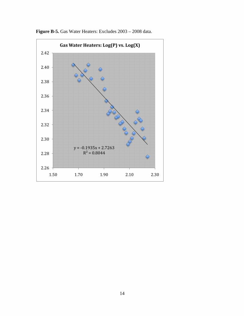
Figure 2 summarizes the results of the analyses, detailed in Table 1. For the majority of products studied the model gives a good fit to the data (see Appendix B). It fails for gas water heaters in recent years (2003 – 2008) during which average producer prices increased. This can be seen by comparing Figures B-5 and B-6 in Appendix B. While examination of causal factors is beyond the scope of this work, a number of factors unrelated to production costs appear to have been involved.

Figure 2. Learning rates for various appliances.

1 Price and shipments data used in product-specific energy efficiency standards rulemakings may differ from the data used in this report.

0 0.1 0.2 0.3 0.4 0.5 0.6

CFLs

Refrigerators

Computers

Cloths washers

Room AC

Freezers

Unitary AC

Electric Water Heaters

Gas Water Heaters

5

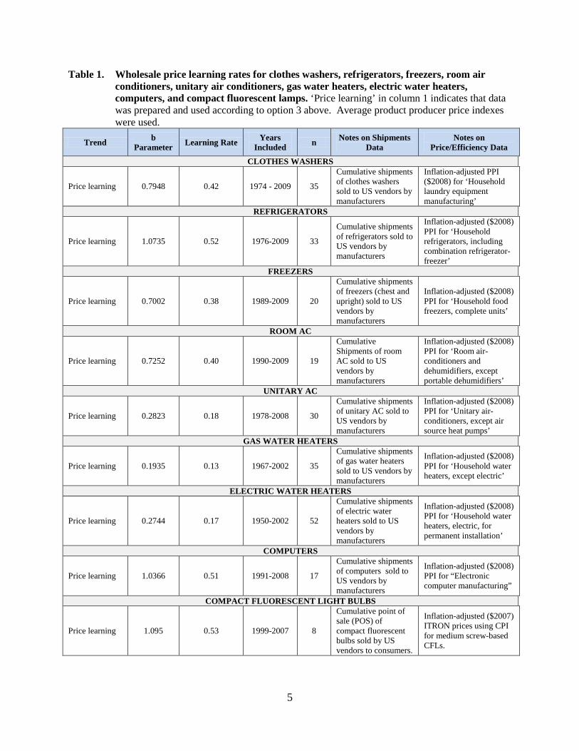
Table 1. Wholesale price learning rates for clothes washers, refrigerators, freezers, room air conditioners, unitary air conditioners, gas water heaters, electric water heaters, computers, and compact fluorescent lamps. ‘Price learning’ in column 1 indicates that data was prepared and used according to option 3 above. Average product producer price indexes were used.

Trend b Parameter Learning Rate Years

Included n Notes on Shipments Data

Notes on Price/Efficiency Data

CLOTHES WASHERS

Price learning 0.7948 0.42 1974 - 2009 35

Cumulative shipments of clothes washers sold to US vendors by manufacturers

Inflation-adjusted PPI ($2008) for ‘Household laundry equipment manufacturing’

REFRIGERATORS

Price learning 1.0735 0.52 1976-2009 33

Cumulative shipments of refrigerators sold to US vendors by manufacturers

Inflation-adjusted ($2008) PPI for ‘Household refrigerators, including combination refrigerator-freezer’

FREEZERS

Price learning 0.7002 0.38 1989-2009 20

Cumulative shipments of freezers (chest and upright) sold to US vendors by manufacturers

Inflation-adjusted ($2008) PPI for ‘Household food freezers, complete units’

ROOM AC

Price learning 0.7252 0.40 1990-2009 19

Cumulative Shipments of room AC sold to US vendors by manufacturers

Inflation-adjusted ($2008) PPI for ‘Room air-conditioners and dehumidifiers, except portable dehumidifiers’

UNITARY AC

Price learning 0.2823 0.18 1978-2008 30

Cumulative shipments of unitary AC sold to US vendors by manufacturers

Inflation-adjusted ($2008) PPI for ‘Unitary air-conditioners, except air source heat pumps’

GAS WATER HEATERS

Price learning 0.1935 0.13 1967-2002 35

Cumulative shipments of gas water heaters sold to US vendors by manufacturers

Inflation-adjusted ($2008) PPI for ‘Household water heaters, except electric’

ELECTRIC WATER HEATERS

Price learning 0.2744 0.17 1950-2002 52

Cumulative shipments of electric water heaters sold to US vendors by manufacturers

Inflation-adjusted ($2008) PPI for ‘Household water heaters, electric, for permanent installation’

COMPUTERS

Price learning 1.0366 0.51 1991-2008 17

Cumulative shipments of computers sold to US vendors by manufacturers

Inflation-adjusted ($2008) PPI for “Electronic computer manufacturing”

COMPACT FLUORESCENT LIGHT BULBS

Price learning 1.095 0.53 1999-2007 8

Cumulative point of sale (POS) of compact fluorescent bulbs sold by US vendors to consumers.

Inflation-adjusted ($2007) ITRON prices using CPI for medium screw-based CFLs.

6

References Bass, F. M. (1980). The Relationship between Diffusion Rates, Experience Curves, and Demand Elasticities for Consumer Durable Technological Innovations. Journal of Business 53:S51-67

Dale, L., C. Antinori, M. McNeil, J.E. McMahon, and K.S. Fujita (2009). Retrospective evaluation of appliance price trends, Energy Policy. 37:597–605. Ellis, M., Jollands, N., Harrington, and L., and Meier, A., (2007). Do energy efficient appliances cost more?, ECEEE 2007 Summer Study. Junginger, M., A. Faaij, and W.C. Turkenburg (2005). Global experience curves for wind farms, Energy Policy: 33:133–150. Greaker, M. and E.L. Sagen (2008). Explaining experience curves for new energy technologies: A case study of liquefied natural gas, Energy Economics. 30:2899–2911 McDonald, A and L. Schrattenholzer, (2001). Learning rates for energy technologies, Energy Policy. 29:255–261. Neij, L. (2008) Cost development of future technologies for power generation—A study based on experience curves and complementary bottom-up assessments. Energy Policy 36: 2200– 2211. Newell, R.G. (2000). Incorporation of Technological Learning into NEMS Buildings Modules, Energy Information Administration. OECD/IEA (2000). Experience Curves for Energy Technology Policy, Organization for Economic Cooperation and Development and the International Energy Agency. Pulliam, R., 2008. California Residential Efficiency Market Share Tracking: Lamps 2007. Prepared for Southern California Edison by Itron, Inc., San Diego, CA. Van Benthem, A., K. Gillingham, and J. Sweeney (2008). Learning-by-Doing and the Optimal Solar Policy in California, The Energy Journal. 29:131–151. Weiss, M, K. Martin, M.K. Patel, M. Junginger, and K. Blok (2010b). Analyzing price and efficiency dynamics of large appliances with the experience curve approach. Energy Policy. 38:770–783. Weiss, M., H.M Junginger, M.K. Patel, and K Blok, (2010a). A review of experience curve analyses for energy demand technologies. Technological Forecasting & Social Change. 77:411-428

7

Appendix A This appendix illustrates how cumulative production (going into US markets) was estimated from domestic shipments histories. The majority of shipments data were obtained from published DOE Technical Support Documents published in support of energy conservation standards. These data rely heavily on Appliance Magazine yearly summaries for residential appliances, and on Association of Home Appliance Manufacturers (AHAM) “Annual Shipment Trends” reports. Data from the Air-Conditioning, Heating and Refrigeration Institute (AHRI) were also used when available and needed. For natural gas appliances, we also use some historical data from the Gas Appliance Manufacturers Association (GAMA). For CFLs shipments data are from a recent market characterization report (Pulliam, 2008). Shipments can typically be linearly extrapolated backwards in time to extend the history back to the theoretical first unit of production. Cumulative production at any given year is then estimated by summing shipments in all prior years, using the linear extrapolation in years before actual data are available. In some cases, if data are shipments data are highly non-linear, this cold give an illogical result, and the plot should be forced to cross the x axis at a logical date for initial production. In the cases shown below, this was necessary only for the freezer data. Figure A-1 plots the results for this analysis for clothes washers, refrigerators, freezers, room and unitary AC, and gas and electric water heaters.

8

Figure A-1. Shipments history for appliances considered in this report. The shipments history has

been extrapolated backward in time to obtain a complete cumulative history. In the case of freezers, only the shipments from 1960-1972 were used in the extrapolation (denoted with red data points).

0

2

4

6

8

0

2

4

6

8

0

4

8

12

0

4

8

12

0

4

8

12

0

2

4

6

8

0

2

4

6

8

0

20

40

60

80

0

20

40

60

1930 1940 1950 1960 1970 1980 1990 2000 2010

Ship

men

ts (i

n m

illio

ns)

Refrigerator

Room AC

Unitary

Freeze

Electric Water Heater

Computers

Gas Water

Clothes Washer

Compact Fluorescent Bulbs

9

Appendix B The following pages document, in turn, the regression analyses for products for which both average product price and average product efficiency were available.

• Clothes washers • Refrigerators • Freezers • Room AC • Gas Water Heaters • Electric Water Heaters

10

Figure B-1. Cloths washers, all data included.

y = -0.7948x + 4.0983R² = 0.97507

2.00

2.10

2.20

2.30

2.40

2.50

2.60

1.80 2.00 2.20 2.40 2.60

Cloths Washes: Log(P) vs. Log(X)

11

Figure B-2. Refrigerators: all data included.

y = -1.0735x + 4.7432R² = 0.97417

1.80

1.90

2.00

2.10

2.20

2.30

2.40

2.50

2.00 2.20 2.40 2.60 2.80

Refrigerators: Log(P) vs. Log(X)

12

Figure B-3. Freezers: all data included.

y = -0.7002x + 3.4814R² = 0.8846

2.08

2.10

2.12

2.14

2.16

2.18

2.20

2.22

2.24

2.26

2.28

2.30

1.70 1.75 1.80 1.85 1.90 1.95 2.00

Freezers: Log(P) vs. Log(X)

13

Figure B-4. Room Air Conditioners: all data included.

y = -0.7252x + 3.7605R² = 0.96937

2.00

2.05

2.10

2.15

2.20

2.25

2.30

2.35

2.00 2.10 2.20 2.30 2.40

Room AC: Log(P) vs. Log(X)

14

Figure B-5. Gas Water Heaters: Excludes 2003 – 2008 data.

y = -0.1935x + 2.7263R² = 0.8044

2.26

2.28

2.30

2.32

2.34

2.36

2.38

2.40

2.42

1.50 1.70 1.90 2.10 2.30

Gas Water Heaters: Log(P) vs. Log(X)

15

Figure B-6. Gas Water Heaters: all data included.

y = -0.0835x + 2.5178R² = 0.15636

2.26

2.28

2.30

2.32

2.34

2.36

2.38

2.40

2.42

2.44

2.46

1.50 1.70 1.90 2.10 2.30 2.50

Gas Water Heaters: Log(P) vs. Log(X)

16

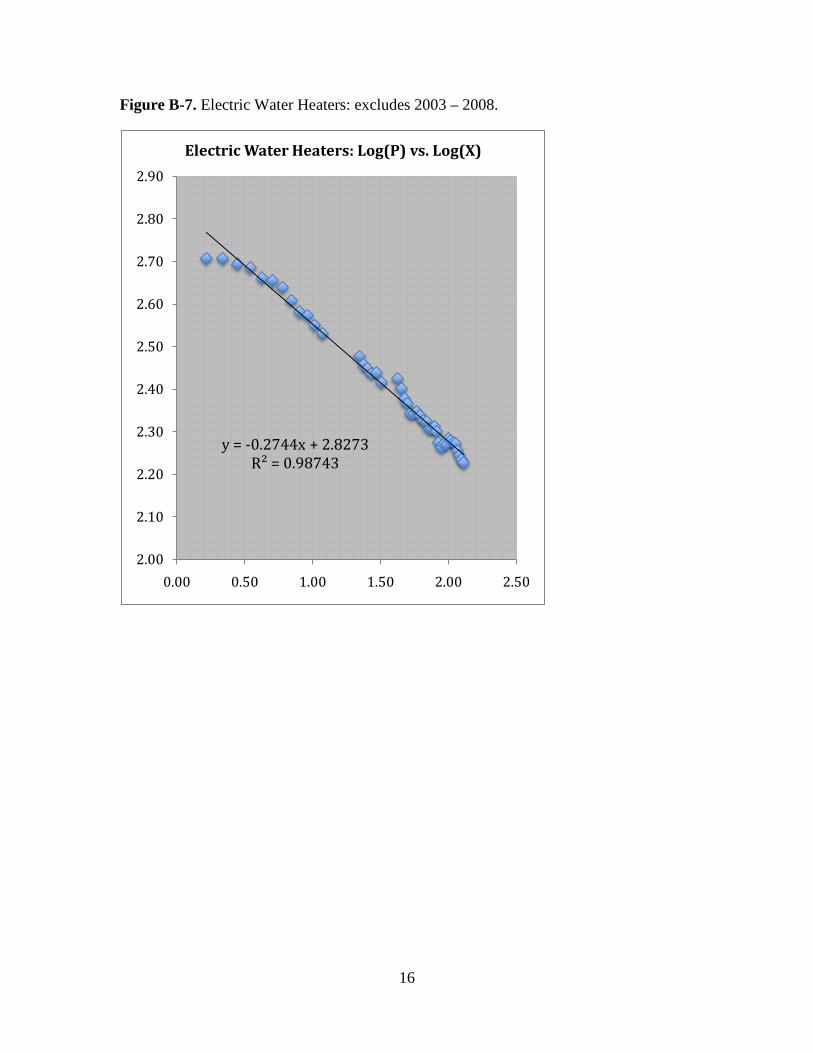
Figure B-7. Electric Water Heaters: excludes 2003 – 2008.

y = -0.2744x + 2.8273R² = 0.98743

2.00

2.10

2.20

2.30

2.40

2.50

2.60

2.70

2.80

2.90

0.00 0.50 1.00 1.50 2.00 2.50

Electric Water Heaters: Log(P) vs. Log(X)