Using the acoustic Doppler current profiler (ADCP) to ... · The acoustic Doppler current profiler...

Study on acoustics for SSC measurements

Using the acoustic Doppler current profiler (ADCP) to

estimate suspended sediment concentration

Technical Report

CPSD #04-01

Yong H. Kim, Benjamin Gutierrez, Tim Nelson, Anton Dumars, Mauro Maza, Hector Perales, and George Voulgaris

Coastal Processes Sediment Dynamics Laboratory Department of Geological Sciences

University of South Carolina Columbia, SC

December 2004

ADCP Calibration (Dec. 2004) CPSD technical report #04-01

i

CONTENTS

1. Introduction ................................................................................................................................. 1

2. Background ................................................................................................................................. 2

2.1. The Sonar Equation.............................................................................................................. 2

2.2. Sound Attenuation................................................................................................................ 4

3. Calibration ................................................................................................................................... 7

3.1. Laboratory Calibration Technique ....................................................................................... 8

3.2. Calibration from Field Data ............................................................................................... 11

4. Inversion.................................................................................................................................... 12

5. Examples ................................................................................................................................... 13

5.1. Data description ................................................................................................................. 13

5.2. Calibration.......................................................................................................................... 14

5.3. Inversion............................................................................................................................. 17

6. References ................................................................................................................................. 19

Appendix ....................................................................................................................................... 20


1

Using the Acoustic Doppler Current Profiler to Estimate Suspended

Sediment Concentration

Coastal Processes and Sediment Dynamics Lab

Department of Geological Sciences

University of South Carolina

Columbia, SC, 29208

1. Introduction

The acoustic Doppler current profiler (ADCP) uses acoustic waves to measure current velocity

profiles in rivers, estuaries, and the ocean. This is accomplished by measuring the frequency shift,

via the Doppler effect, of sound backscattered from particles (scatterers) in the water. The

intensity of the sound that is backscattered off particles is related to suspended sediment

concentration (SSC) through a calibration procedure. Investigators have devised techniques to

estimate SSC by using the backscatter intensity measured by the ADCP (e.g., Holdaway et al.,

1999; Kim and Voulgaris, 2003; Gartner, 2004). This approach is similar to the use of higher-

frequency, acoustic backscatterance sensors (ABS, for a review see Thorne and Hanes, 2002)

developed specifically for suspended sediment concentration measurements.

Calibration procedure described within this report enables investigators to expand the utility of

the ADCP to include suspended sediment concentration estimates through the water column.

Suspended sediment concentration (SSC) estimates using ADCP are acquired through greater

flow depths than transmissometers, laser in-situ scatterometery (LISST), and optical

backscatterance sensors (OBS), whose sample ranges are significantly shorter. However,

simultaneous, although limited, use of one of these methods is necessary for calibrating the

ADCP to provide accurate SSC estimates. In addition, ADCP-derived SSC records continuously

through the water column, which may prove more advantageous than discrete-depth direct bottle

sampling.

Within this document we outline the method that was developed to calibrate the Broad Band

ADCP to estimate SSC. In Section 2 a brief background detailing the theoretical basis from which

the approach was derived is presented. Our calibration equation is modified from the initial

approach by Deines (1999), where he developed the working version of sonar equation applicable

to the ADCP. The most significant progress by this study is that we add the term relating the

attenuation due to sediment that was not accounted for in Deines (1999). The calibration

procedure is explained in section 3. Section 4 describes the inversion process, which is a critical


2

and sometimes complicated step in estimating an accurate sediment concentration profile. Finally,

Section 5 provides examples for use as a guide to the calibration process. Lastly, the MATLAB®

functions developed for both the calibration and inversion methods are included as appendices.

2. Background

2.1. The Sonar Equation

The active sonar equation is used to relate acoustic backscatter intensity (measured with the

ADCP) to suspended sediment concentration. Since some of variables in the basic sonar equation

cannot be measured independently, Deines (1999) developed a working version of sonar equation

for an ADCP. A ping from an ADCP, in its two-way travel, has several stages: Transmission -

radiating signal - backscattering - returning echo - reception. In terms of the power (energy) of

the pulse, the signal (S) to noise (N) ratio can be expressed as follows (Deines, 1999):

[ ]FBTK

EG

R

tcR

R

GEP

N

S

N

X

RSv

RXE

⋅⋅⋅⋅⋅

⋅

⋅⋅⋅⋅

⋅⋅

⋅⋅⋅⋅⋅

⋅

⋅=

⋅−⋅− 1

410

10

2410

4

2

10

2

102

10

2 π

λϕπ

π

αα

(1)

where PE is electrical power to transducer (in W), EX is transducer efficiency, G is transducer gain

or directivity, R is range to scatterers along the beam (in m), α stands for water absorption

(in dB m-1

), φ is effective two-way beam width (in radians), c is speed of sound (in m s-1

), t is

transmit pulse length (in s), Sv is backscatterering strength (in dB [4π m] -1

), λ is wavelength of

transmitter (in m), K is Boltzmann's constant (1.38·10-23

joules ºK-1

), T is temperature at the

transducer (in ºK), BN is noise bandwidth (in Hz), F is receiver noise factor, and D is transducer

diameter (in m).

The first term on the right hand side gives the power density of the transmitter, which is (1)

considered a point source, (2) measured a meter away from the source, and (3) corrected by the

efficiency. This term accounts for the transmission in the conceptual presentation. The 2nd

and 3rd

terms consider the radiation conditions. The second term expresses the way the signal is radiated

(directivity) and considers the decay of the signal strength with distance. The third term takes into

account for the losing due to absorption (in one way). Terms fourth to sixth measure the

backscattering, given the volume ensonified (4th × 5

th) and corrected by the retro-dispersion

properties of the scatterers (6th). The echo attenuation in his way back to the sensor, which is

same as term 3, is accounted by the 7th term. The 8

th term accounts for the capture area and the

efficiency is considered again by multiplying the 9th term. Therefore terms from 1

st to 9

th


3

represent the received signal power, which is finally divided by the noise properties of the

detector (10th term).

Using the following expressions for the directivity

2

⋅=

λ

π dG , the effective two-way beam

width

2

2

2

4

⋅⋅

⋅=

dπ

λϕ , transmit pulse length

c

Lt

⋅

⋅=

θcos

2, the noise in terms of the

temperature NBTKN ⋅⋅= , and signal to noise power ratio measured by RDI ADCP

( )1010

rc EEK

N

S −⋅

= , the equation 1 can be re-arranged for the backscattering strength (Sv) (Deines,

1999):

( ) )(2log10 2

rcDBWDBMv EEKRPLRTCS −⋅+⋅⋅+−−⋅⋅+= α (2)

where LDBM is 10log10(L), PDBW is 10log10(PE), Kc is Received Signal Strength Indicator (RSSI)

scale factor (in dB count-1

), E is echo strength (in count), Er is received noise (in counts), and

C is

⋅⋅

⋅⋅⋅⋅⋅

22

cos8log10

dE

BFK

X

N

π

θ. Thus the last constant depends on the characteristics of the

acoustic system employed.

The method discussed until now describes theoretical approach to calculate the constant C.

However, if we have the sediment concentration data measured simultaneously, the constants C

and Kc can be estimated by interpolating the measured SSC from (Deines, 1999):

( ) )(2log20 10 rcDBWDBMv EEKRPLRCC −⋅+⋅⋅+−−⋅+= α (3)

where the symbols are as before and Cv is )log(10 SSC⋅ . In the calibration procedure outlined in

Kim and Voulgaris (2003) the terms C and Kc are determined by linear regression between

backscatter intensity from a RDI ADCP and sediment concentrations measured simultaneously,

with an OBS.

In the working version of sonar equations in Deines (1999), the attenuation due to suspended

particles was not accounted for. When the attenuation due to sediments is included in sonar

equation, the two-way transmission loss (2TL) can be calculated by

RARTL sw ⋅+⋅+⋅=⋅ )(2)(log202 10 α (4)


4

where αw is the water absorption coefficients and As is the sound attenuation due to sediments.

The first term in this equation, 20log(R), is the loss due to beam spreading. The remaining terms

are the losses due to acoustic absorption due to water and sediment, respectively, which are

described in more detail in section 2.2.

In this report we add the sediment absorption term to the simplified sonar equation for RDI

ADCP (equation 3), to yield:

( ) )(2)(log10)(log10 2

1010 rcDBWDBMsw EEKPLRARCSSC −⋅+−−⋅+⋅+⋅+=⋅ α

(5)

where the symbols are as before. The calibration procedure introduced in this document is used to

estimate the terms C and Kc in this expression using two approaches. In one of these methods, Kc

is determined in the laboratory, while in the other method, both terms, C and Kc, are determined

by linear regression of backscatter intensity to sediment concentrations measured in the field with

an OBS or other methods (LISST or bottle sampling). The latter can be done using the following

reduced form of equation 5:

CEEKSSC rcv +−⋅= )( (6)

where ( ) DBWDBMswv PLRARSSCSSC ++⋅+⋅−⋅−⋅= α2)(log20)(log10 1010 . This

procedure is explained in greater detail in section 3.2 and examples are given in section 5.

2.2. Sound Attenuation

Two important terms introduced in the previous section were the attenuation of sound in water

(αw) and attenuation of sound due to suspended sediment (As). Attenuation due to water is a

function of transmitting frequency, salinity and temperature of water, and pressure. Sound

absorption in clear seawater involves the combined effects of absorption due to pure water and

the effects of ionic relaxation process of both boric acid and magnesium sulfate (Richards et al,

1996). A commonly used equation for calculating αw (in dB m-1

) is as follows

( )

⋅⋅+

+

⋅⋅⋅+

+

⋅⋅⋅⋅= 2

3322

2

2

222

22

1

2

112log10 fPAff

ffPA

ff

ffAewα (7)


5

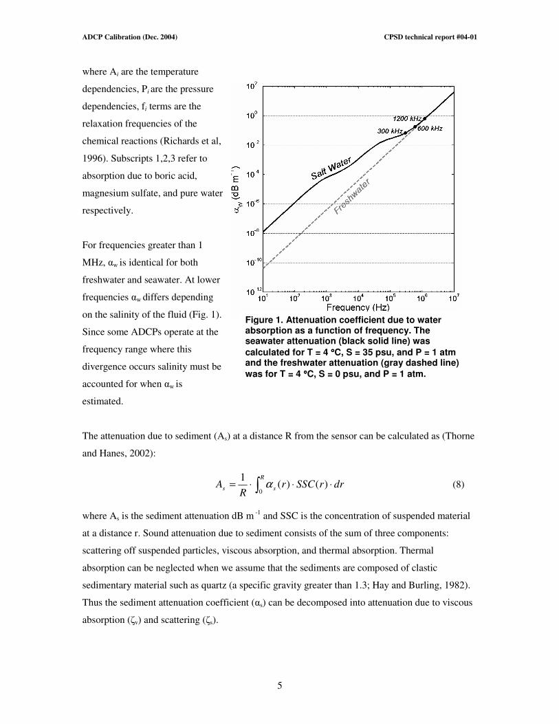
where Ai are the temperature

dependencies, Pi are the pressure

dependencies, fi terms are the

relaxation frequencies of the

chemical reactions (Richards et al,

1996). Subscripts 1,2,3 refer to

absorption due to boric acid,

magnesium sulfate, and pure water

respectively.

For frequencies greater than 1

MHz, αw is identical for both

freshwater and seawater. At lower

frequencies αw differs depending

on the salinity of the fluid (Fig. 1).

Since some ADCPs operate at the

frequency range where this

divergence occurs salinity must be

accounted for when αw is

estimated.

The attenuation due to sediment (As) at a distance R from the sensor can be calculated as (Thorne

and Hanes, 2002):

∫ ⋅⋅⋅=R

ss drrSSCrR

A0

)()(1

α (8)

where As is the sediment attenuation dB m -1

and SSC is the concentration of suspended material

at a distance r. Sound attenuation due to sediment consists of the sum of three components:

scattering off suspended particles, viscous absorption, and thermal absorption. Thermal

absorption can be neglected when we assume that the sediments are composed of clastic

sedimentary material such as quartz (a specific gravity greater than 1.3; Hay and Burling, 1982).

Thus the sediment attenuation coefficient (αs) can be decomposed into attenuation due to viscous

absorption (ζv) and scattering (ζs).

Figure 1. Attenuation coefficient due to water absorption as a function of frequency. The seawater attenuation (black solid line) was

calculated for T = 4 °°°°C, S = 35 psu, and P = 1 atm and the freshwater attenuation (gray dashed line)

was for T = 4 °°°°C, S = 0 psu, and P = 1 atm.


6

First, the viscous absorption occurs when there is a difference between the particle density and

the surrounding fluid density. The difference in density produces a difference in inertial forces,

which in turn, results in a velocity gradient between the particle and the fluid in which it is

suspended. Due to the relative motion between the two, a boundary layer is formed around the

particle, leading to damping of the relative motion of the particle (Richards, 2003). The following

equation was developed by Urick (1948):

( )

( )

++⋅

−⋅⋅⋅⋅=

22

2

2

2

1)log10(

δσ

σες

s

skev (9)

where

⋅+⋅

⋅⋅=

ss aas

ββ

11

4

9,

⋅⋅+⋅=

saβδ

2

91

2

1,

0ρ

ρσ s= ,

21

2

⋅=

ν

ωβ is oscillatory boundary layer depth, ε is the volume concentration of scatterers, k

is the acoustic wavenumber, σ is the ratio of the densities of the solid and fluid phases, <as> is the

mean particle radius, ρs is the density of sediment, ρo is the density of water, υ is the kinematic

viscosity of water, and ω = 2πf, where f is operating frequency of the ADCP. So, as acoustic

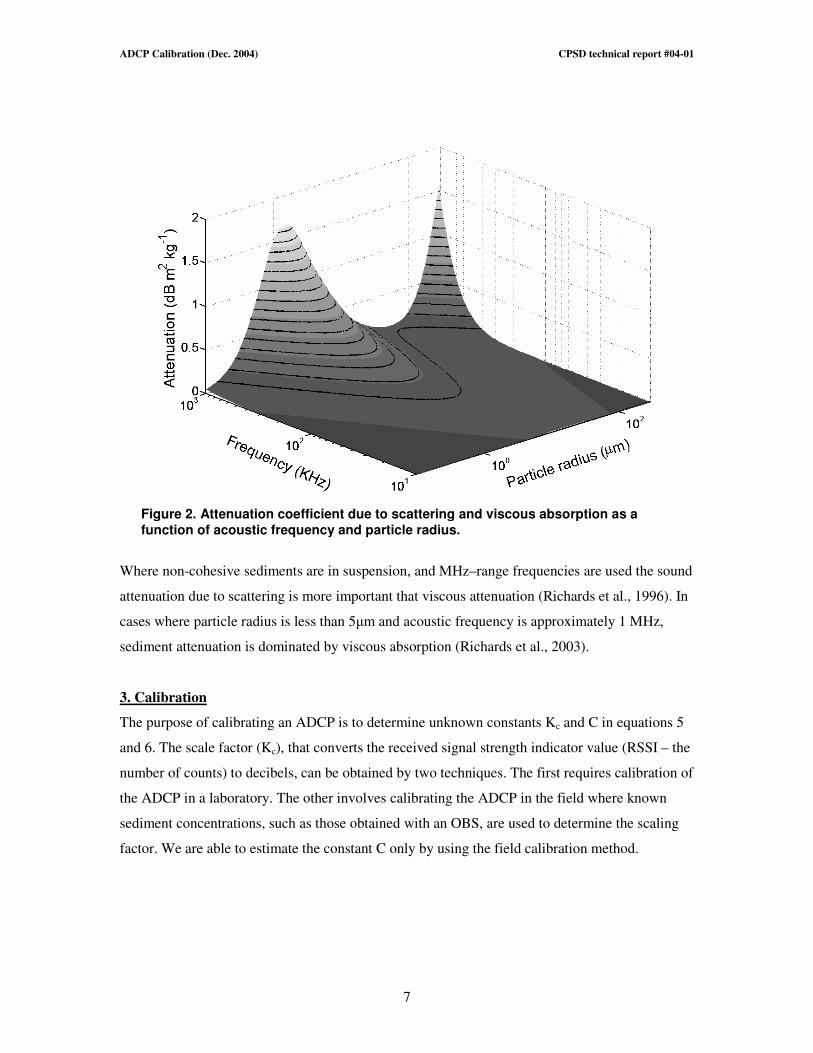
frequency increases, viscous absorption increases (Fig. 2). In contrast, viscous absorption

decreases as particle size increases (for grains >10µm; Richards et al, 1996; Fig. 2).

Second, the attenuation coefficient due to scattering can be calculated by the following equation

(Richards et al., 1996)

( )( )

⋅⋅+⋅+⋅

⋅⋅⋅⋅=

4222

34

2

24.01log10

sss

s

s

akak

ake

ρ

ες (10)

Where, the symbols are as before. Scattering losses increase as sediment grain size increases, as

well as a function of wavelength (λ) and particle circumference 2πas. When λ >>2πas, most of the

scattering pattern propagates backward. When λ<<2πas, half the scattered pattern propagates

forward and the remainder is scattered in all directions (Flammers, 1962).


7

Where non-cohesive sediments are in suspension, and MHz–range frequencies are used the sound

attenuation due to scattering is more important that viscous attenuation (Richards et al., 1996). In

cases where particle radius is less than 5µm and acoustic frequency is approximately 1 MHz,

sediment attenuation is dominated by viscous absorption (Richards et al., 2003).

3. Calibration

The purpose of calibrating an ADCP is to determine unknown constants Kc and C in equations 5

and 6. The scale factor (Kc), that converts the received signal strength indicator value (RSSI – the

number of counts) to decibels, can be obtained by two techniques. The first requires calibration of

the ADCP in a laboratory. The other involves calibrating the ADCP in the field where known

sediment concentrations, such as those obtained with an OBS, are used to determine the scaling

factor. We are able to estimate the constant C only by using the field calibration method.

Figure 2. Attenuation coefficient due to scattering and viscous absorption as a

function of acoustic frequency and particle radius.


8

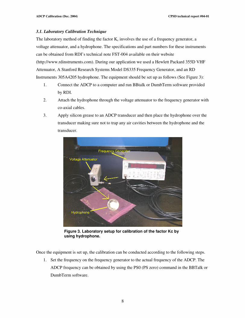
3.1. Laboratory Calibration Technique

The laboratory method of finding the factor Kc involves the use of a frequency generator, a

voltage attenuator, and a hydrophone. The specifications and part numbers for these instruments

can be obtained from RDI’s technical note FST-004 available on their website

(http://www.rdinstruments.com). During our application we used a Hewlett Packard 355D VHF

Attenuator, A Stanford Research Systems Model DS335 Frequency Generator, and an RD

Instruments 305A4205 hydrophone. The equipment should be set up as follows (See Figure 3):

1. Connect the ADCP to a computer and run BBtalk or DumbTerm software provided

by RDI.

2. Attach the hydrophone through the voltage attenuator to the frequency generator with

co-axial cables.

3. Apply silicon grease to an ADCP transducer and then place the hydrophone over the

transducer making sure not to trap any air cavities between the hydrophone and the

transducer.

Once the equipment is set up, the calibration can be conducted according to the following steps.

1. Set the frequency on the frequency generator to the actual frequency of the ADCP. The

ADCP frequency can be obtained by using the PS0 (PS zero) command in the BBTalk or

DumbTerm software.

Figure 3. Laboratory setup for calibration of the factor Kc by using hydrophone.


9

2. Send a PT103 command to the ADCP. This causes the RSSI value to be continuously

displayed on the computer.

3. Next set the peak-to-peak voltage (Vpp) value on the frequency generator to 0.05 volts

and the attenuator to 0 dB.

4. Record the RSSI value for this setting.

5. Increase the attenuation (hereafter termed as Atn) by 10 dB and again record the value.

6. Repeat step 5 until the RSSI value no longer decreases with increasing attenuation. This

RSSI value is called the reference level (Er) and according to Deines (1999) has a value

of about 40 counts. In our lab calibration, the value was approximately 48 counts for the

three ADCPs that we tested.

7. Next, increase the peak-to-peak voltage. From our experience we found that using

voltages of 0.05, 0.1, 0.5, 1, 1.5, 2.5, 5, and 7.5 volts while changing the attenuator

setting (Atn) at 0 to 50 dB for 0.05 and 0.1 volts while keeping the attenuation at 0 dB for

the remaining provides a reasonable range of values. If needed the voltage can be

increased farther until the maximum number of counts has been reached. We found the

RSSI values to level off at approximately 5 volts for most of the transducers that we

tested in the lab. Detail data of our lab calibration method are listed in Table 1.

8. Once these values are obtained, the volts are converted into decibels (VdB) using the

equation

AtnV

VV

ref

pp

dB −

⋅= log20 (11)

where Vref is the lowest Vpp value used and Atn represents attenuation in dB. For

example, if the lowest Vpp used was 0.05 and you are solving for a Vpp of 0.1 volts with

an attenuation of 20 dB the equation would be

dBVdb 97.132005.0

1.0log10 −=−

= (12)

9. Once a list of voltages in dB is found for a given number of counts, VdB is plotted versus

RSSI using only the data that falls between and the first value at the maximum and

minimum detectable RSSI value (see Tabel 1 and Figure 2). A best-fit line is then

calculated by linear regression to determine the slope of the line (Kc) from

BRSSIKV cdb +⋅= (13)


10

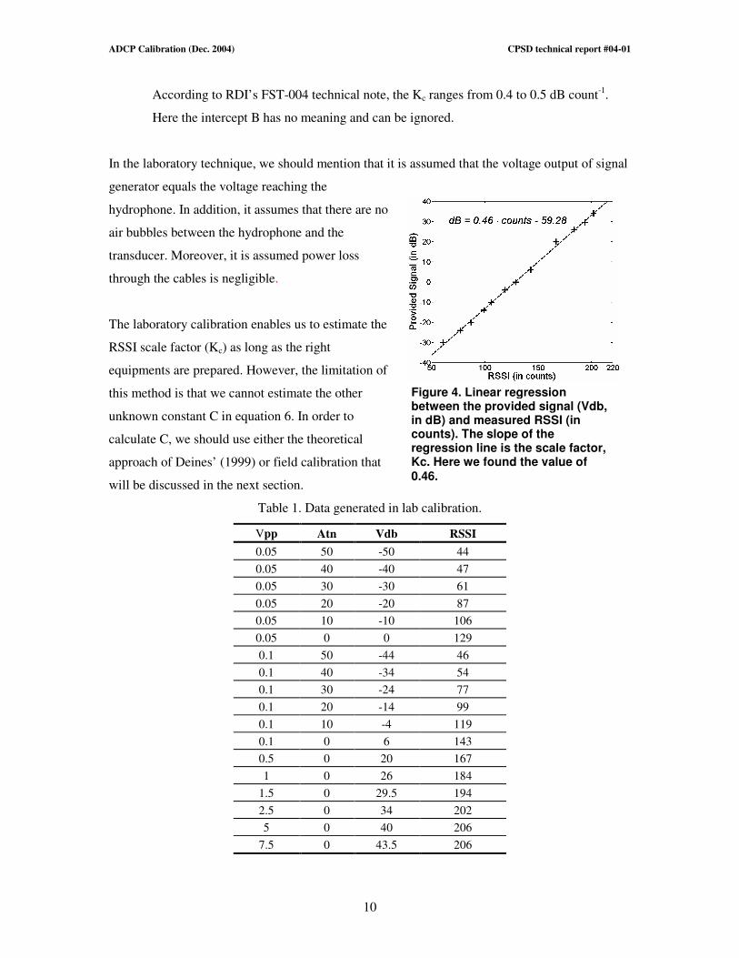
Figure 4. Linear regression between the provided signal (Vdb, in dB) and measured RSSI (in counts). The slope of the regression line is the scale factor, Kc. Here we found the value of 0.46.

According to RDI’s FST-004 technical note, the Kc ranges from 0.4 to 0.5 dB count-1

.

Here the intercept B has no meaning and can be ignored.

In the laboratory technique, we should mention that it is assumed that the voltage output of signal

generator equals the voltage reaching the

hydrophone. In addition, it assumes that there are no

air bubbles between the hydrophone and the

transducer. Moreover, it is assumed power loss

through the cables is negligible.

The laboratory calibration enables us to estimate the

RSSI scale factor (Kc) as long as the right

equipments are prepared. However, the limitation of

this method is that we cannot estimate the other

unknown constant C in equation 6. In order to

calculate C, we should use either the theoretical

approach of Deines’ (1999) or field calibration that

will be discussed in the next section.

Table 1. Data generated in lab calibration.

Vpp Atn Vdb RSSI

0.05 50 -50 44

0.05 40 -40 47

0.05 30 -30 61

0.05 20 -20 87

0.05 10 -10 106

0.05 0 0 129

0.1 50 -44 46

0.1 40 -34 54

0.1 30 -24 77

0.1 20 -14 99

0.1 10 -4 119

0.1 0 6 143

0.5 0 20 167

1 0 26 184

1.5 0 29.5 194

2.5 0 34 202

5 0 40 206

7.5 0 43.5 206


11

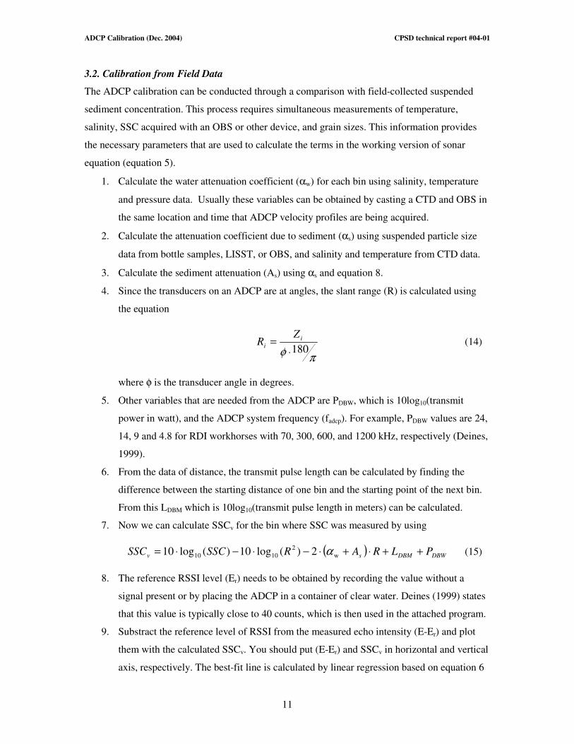
3.2. Calibration from Field Data

The ADCP calibration can be conducted through a comparison with field-collected suspended

sediment concentration. This process requires simultaneous measurements of temperature,

salinity, SSC acquired with an OBS or other device, and grain sizes. This information provides

the necessary parameters that are used to calculate the terms in the working version of sonar

equation (equation 5).

1. Calculate the water attenuation coefficient (αw) for each bin using salinity, temperature

and pressure data. Usually these variables can be obtained by casting a CTD and OBS in

the same location and time that ADCP velocity profiles are being acquired.

2. Calculate the attenuation coefficient due to sediment (αs) using suspended particle size

data from bottle samples, LISST, or OBS, and salinity and temperature from CTD data.

3. Calculate the sediment attenuation (As) using αs and equation 8.

4. Since the transducers on an ADCP are at angles, the slant range (R) is calculated using

the equation

πφ 180⋅

= i

i

ZR (14)

where φ is the transducer angle in degrees.

5. Other variables that are needed from the ADCP are PDBW, which is 10log10(transmit

power in watt), and the ADCP system frequency (fadcp). For example, PDBW values are 24,

14, 9 and 4.8 for RDI workhorses with 70, 300, 600, and 1200 kHz, respectively (Deines,

1999).

6. From the data of distance, the transmit pulse length can be calculated by finding the

difference between the starting distance of one bin and the starting point of the next bin.

From this LDBM which is 10log10(transmit pulse length in meters) can be calculated.

7. Now we can calculate SSCv for the bin where SSC was measured by using

( ) DBWDBMsv PLRARSSCSSC ++⋅+⋅−⋅−⋅= w

2

1010 2)(log10)(log10 α (15)

8. The reference RSSI level (Er) needs to be obtained by recording the value without a

signal present or by placing the ADCP in a container of clear water. Deines (1999) states

that this value is typically close to 40 counts, which is then used in the attached program.

9. Substract the reference level of RSSI from the measured echo intensity (E-Er) and plot

them with the calculated SSCv. You should put (E-Er) and SSCv in horizontal and vertical

axis, respectively. The best-fit line is calculated by linear regression based on equation 6


12

( CEEKSSC rcv +−⋅= )( ), and then and then the slope and the intercept would be

read for Kc and C, respectively.

4. Inversion

The inversion process includes calculating suspended sediment concentration (SSC) from ADCP

echo intensity by using the constants that were obtained from calibration. In Kim and Voulgaris

(2003), for example, the calibration method was evaluated by comparing ADCP- and OBS-

derived SSCs.

Once the constants Kc and C are calculated through the calibration (see Section III), the practical

version of SONAR equation (eq. 5) can be completed and solved for SSC as:

( )

−⋅+−−⋅+⋅+⋅+⋅=

10

)(2)(log20exp10 10 rcDBWDBMsw EEKPLRARC

SSCα

(16)

A SSC calculation algorithm is developed for the evaluation of this equation following the next

steps:

1. Information of temperature and salinity must be assigned for each bin. However, in case

that there is no vertical profile data, a constant temperature and salinity can be used for

calculation assuming well-mixed water column.

2. A mean grain size ( 50D ), must be assigned to each depth. However, in case that there is

no vertical profile data, a constant grain size can also be used.

3. The system parameters of the ADCP (PDBW, LDBM, and Er) are same as what used in

calibration.

4. The water attenuation coefficient (αw, in dB m-1

) is calculated for each bin based on the

known values of temperature, salinity, depth, frequency and Ph.

5. Attenuation due to sediment (As, in dB m2 kg

-1) is also calculated for each bin based on

the known values of water temperature, salinity, depth, frequency of the transducer,

sediment size (mean diameter 50D ), and sediment density.

6. Finally the equation 16 is applied and SSC can be derived from ADCP echo intensity

data.


13

The values obtained from this procedure can be compared with measured values of sediment

concentration obtained from filtered water samples or optical SSC estimates. That comparison

will provide an indication of the quality of our calibration and inversion algorithms.

5. Examples

A case study provided in this section can be used as a guide to the calibration and inversion

processes. For the calibration process in this section, we collected the echo intensity profile from

an ADCP as well as a vertical profile of CTD-OBS-LISST data at the same time. These data were

collected at a field study site located in Winyah Bay near Georgetown, South Carolina. In this

example we estimate the constants Kc and C through the linear regression using the simplified

SONAR equation (see equation 5). After putting the estimated Kc and C value into the equation,

SSC is derived from only ADCP backscatter data by using the equation, and then it is compared

with OBS-derived SSC.

5.1. Data description

One-tidal-day (25 hours) of current, temperature, salinity, SSC and grain size were acquired at a

station (WB6) in the middle part of Winyah Bay estuary, during September 12-13, 2002 (low

freshwater discharge period). A ship-mounted, downward-looking ADCP (RDI Workhorse

Broadband 1200 kHz) recorded current velocities and echo intensities continuously, with a bin

size of 0.25 m. The echo intensity data were collected from 4 beams of the ADCP and then

averaged for each bin. Hydrographic and sedimentological data were also measured by casting an

instrument frame containing a CTD (Ocean Sensors 200), an optical backscatterance sensor

(OBS), and a Laser In-Situ Scattering Transmissometer (LISST). The instrument package was

lowered slowly to the bed and real-time data was transmitted to an onboard computer. The

sampling frequency of all instruments was approximately 1Hz, which resulted in a vertical

resolution of approximately 2.3 cm. All the measured data are vertically averaged over a vertical

spacing of 0.25 m, which is same as the bin size of the ADCP data. Once the instruments were

lowered to the seabed, water samples from three different depths were collected using a

submersible pump while the instrument package was being raised back through the water column.

In order to calculate suspended sediment concentration (SSC), volumes of water ranging from 30

to 300 ml were filtered by pre-weighed and pre-combusted 47-mm diameter GF/F filters with a

nominal 0.7 µm pore size. Filters were stored at –20 °C until we returned to the laboratory where

they were oven-dried at 50 °C for at least 48 hours and reweighed. The sediment concentration

from pumped water samples were used to calibrate the OBS measurements according to:


14

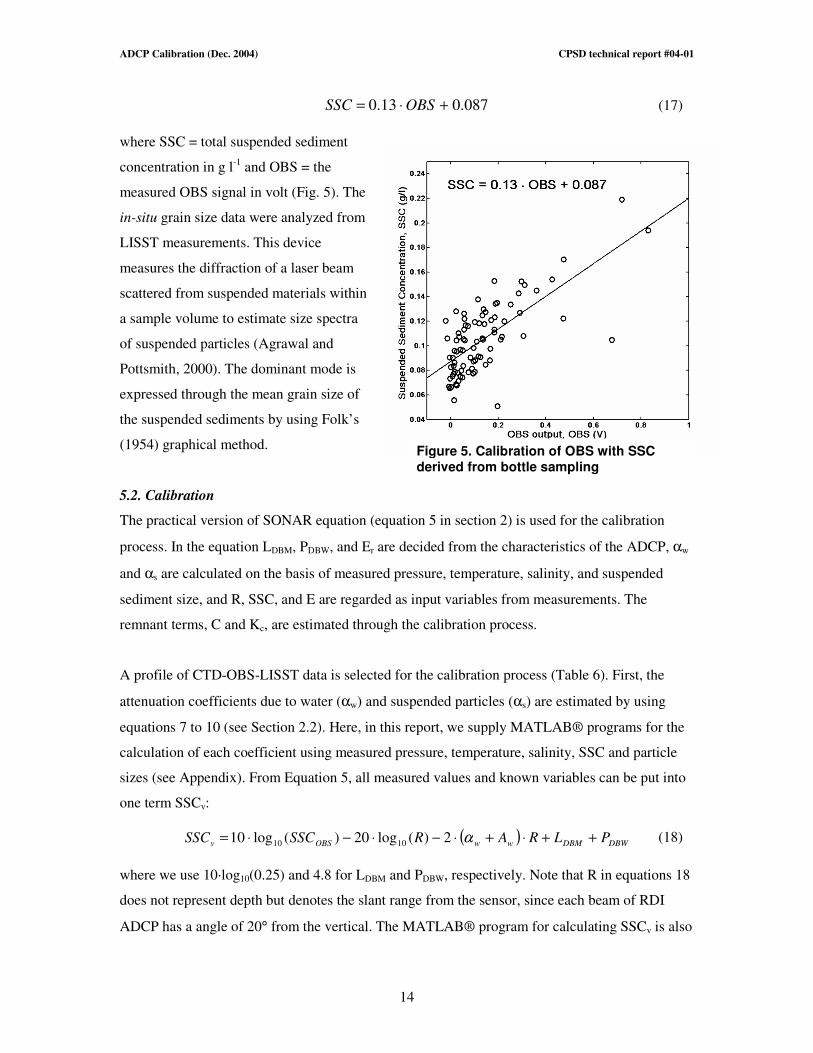
087.013.0 +⋅= OBSSSC (17)

where SSC = total suspended sediment

concentration in g l-1

and OBS = the

measured OBS signal in volt (Fig. 5). The

in-situ grain size data were analyzed from

LISST measurements. This device

measures the diffraction of a laser beam

scattered from suspended materials within

a sample volume to estimate size spectra

of suspended particles (Agrawal and

Pottsmith, 2000). The dominant mode is

expressed through the mean grain size of

the suspended sediments by using Folk’s

(1954) graphical method.

5.2. Calibration

The practical version of SONAR equation (equation 5 in section 2) is used for the calibration

process. In the equation LDBM, PDBW, and Er are decided from the characteristics of the ADCP, αw

and αs are calculated on the basis of measured pressure, temperature, salinity, and suspended

sediment size, and R, SSC, and E are regarded as input variables from measurements. The

remnant terms, C and Kc, are estimated through the calibration process.

A profile of CTD-OBS-LISST data is selected for the calibration process (Table 6). First, the

attenuation coefficients due to water (αw) and suspended particles (αs) are estimated by using

equations 7 to 10 (see Section 2.2). Here, in this report, we supply MATLAB® programs for the

calculation of each coefficient using measured pressure, temperature, salinity, SSC and particle

sizes (see Appendix). From Equation 5, all measured values and known variables can be put into

one term SSCv:

( ) DBWDBMwwOBSv PLRARSSCSSC ++⋅+⋅−⋅−⋅= α2)(log20)(log10 1010 (18)

where we use 10·log10(0.25) and 4.8 for LDBM and PDBW, respectively. Note that R in equations 18

does not represent depth but denotes the slant range from the sensor, since each beam of RDI

ADCP has a angle of 20° from the vertical. The MATLAB® program for calculating SSCv is also

Figure 5. Calibration of OBS with SSC derived from bottle sampling


15

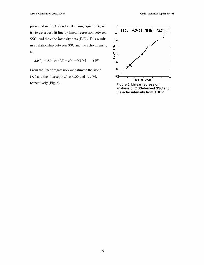
Figure 6. Linear regression analysis of OBS-derived SSC and the echo intensity from ADCP

presented in the Appendix. By using equation 6, we

try to get a best-fit line by linear regression between

SSCv and the echo intensity data (E-Er). This results

in a relationship between SSC and the echo intensity

as

74.72)(5493.0 −−⋅= ErESSCv (19)

From the linear regression we estimate the slope

(Kc) and the intercept (C) as 0.55 and –72.74,

respectively (Fig. 6).


16

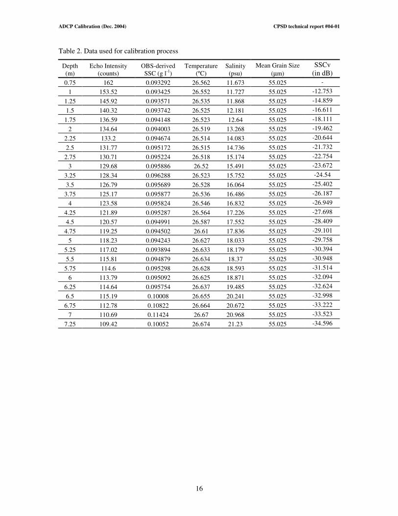
Table 2. Data used for calibration process

Depth

(m)

Echo Intensity

(counts)

OBS-derived

SSC (g l-1

)

Temperature

(ºC)

Salinity

(psu)

Mean Grain Size

(µm)

SSCv

(in dB)

0.75 162 0.093292 26.562 11.673 55.025 -

1 153.52 0.093425 26.552 11.727 55.025 -12.753

1.25 145.92 0.093571 26.535 11.868 55.025 -14.859

1.5 140.32 0.093742 26.525 12.181 55.025 -16.611

1.75 136.59 0.094148 26.523 12.64 55.025 -18.111

2 134.64 0.094003 26.519 13.268 55.025 -19.462

2.25 133.2 0.094674 26.514 14.083 55.025 -20.644

2.5 131.77 0.095172 26.515 14.736 55.025 -21.732

2.75 130.71 0.095224 26.518 15.174 55.025 -22.754

3 129.68 0.095886 26.52 15.491 55.025 -23.672

3.25 128.34 0.096288 26.523 15.752 55.025 -24.54

3.5 126.79 0.095689 26.528 16.064 55.025 -25.402

3.75 125.17 0.095877 26.536 16.486 55.025 -26.187

4 123.58 0.095824 26.546 16.832 55.025 -26.949

4.25 121.89 0.095287 26.564 17.226 55.025 -27.698

4.5 120.57 0.094991 26.587 17.552 55.025 -28.409

4.75 119.25 0.094502 26.61 17.836 55.025 -29.101

5 118.23 0.094243 26.627 18.033 55.025 -29.758

5.25 117.02 0.093894 26.633 18.179 55.025 -30.394

5.5 115.81 0.094879 26.634 18.37 55.025 -30.948

5.75 114.6 0.095298 26.628 18.593 55.025 -31.514

6 113.79 0.095092 26.625 18.871 55.025 -32.094

6.25 114.64 0.095754 26.637 19.485 55.025 -32.624

6.5 115.19 0.10008 26.655 20.241 55.025 -32.998

6.75 112.78 0.10822 26.664 20.672 55.025 -33.222

7 110.69 0.11424 26.67 20.968 55.025 -33.523

7.25 109.42 0.10052 26.674 21.23 55.025 -34.596


17

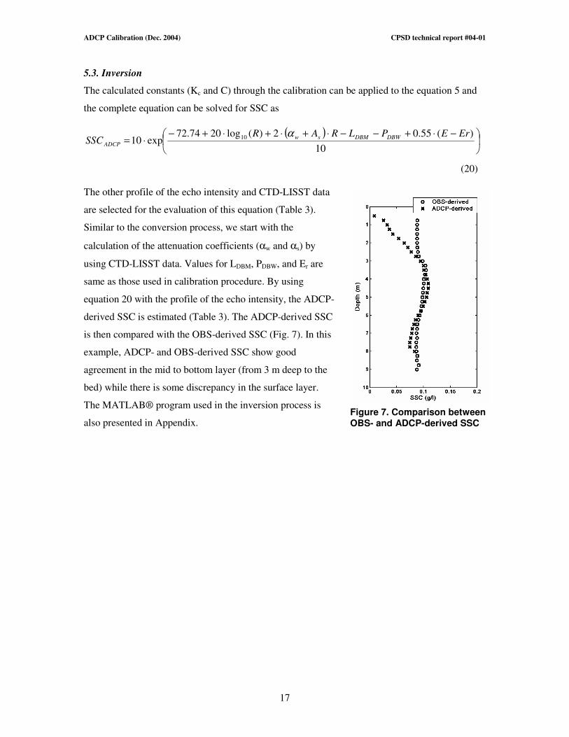
5.3. Inversion

The calculated constants (Kc and C) through the calibration can be applied to the equation 5 and

the complete equation can be solved for SSC as

( )

−⋅+−−⋅+⋅+⋅+−⋅=

10

)(55.02)(log2074.72exp10 10 ErEPLRAR

SSC DBWDBMsw

ADCP

α

(20)

The other profile of the echo intensity and CTD-LISST data

are selected for the evaluation of this equation (Table 3).

Similar to the conversion process, we start with the

calculation of the attenuation coefficients (αw and αs) by

using CTD-LISST data. Values for LDBM, PDBW, and Er are

same as those used in calibration procedure. By using

equation 20 with the profile of the echo intensity, the ADCP-

derived SSC is estimated (Table 3). The ADCP-derived SSC

is then compared with the OBS-derived SSC (Fig. 7). In this

example, ADCP- and OBS-derived SSC show good

agreement in the mid to bottom layer (from 3 m deep to the

bed) while there is some discrepancy in the surface layer.

The MATLAB® program used in the inversion process is

also presented in Appendix.

Figure 7. Comparison between OBS- and ADCP-derived SSC


18

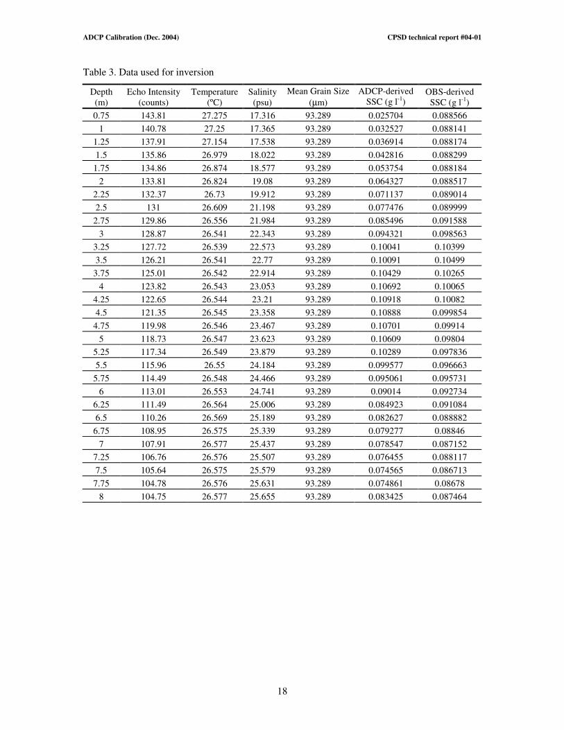
Table 3. Data used for inversion

Depth

(m)

Echo Intensity

(counts)

Temperature

(ºC)

Salinity

(psu)

Mean Grain Size

(µm)

ADCP-derived

SSC (g l-1

) OBS-derived

SSC (g l-1

)

0.75 143.81 27.275 17.316 93.289 0.025704 0.088566

1 140.78 27.25 17.365 93.289 0.032527 0.088141

1.25 137.91 27.154 17.538 93.289 0.036914 0.088174

1.5 135.86 26.979 18.022 93.289 0.042816 0.088299

1.75 134.86 26.874 18.577 93.289 0.053754 0.088184

2 133.81 26.824 19.08 93.289 0.064327 0.088517

2.25 132.37 26.73 19.912 93.289 0.071137 0.089014

2.5 131 26.609 21.198 93.289 0.077476 0.089999

2.75 129.86 26.556 21.984 93.289 0.085496 0.091588

3 128.87 26.541 22.343 93.289 0.094321 0.098563

3.25 127.72 26.539 22.573 93.289 0.10041 0.10399

3.5 126.21 26.541 22.77 93.289 0.10091 0.10499

3.75 125.01 26.542 22.914 93.289 0.10429 0.10265

4 123.82 26.543 23.053 93.289 0.10692 0.10065

4.25 122.65 26.544 23.21 93.289 0.10918 0.10082

4.5 121.35 26.545 23.358 93.289 0.10888 0.099854

4.75 119.98 26.546 23.467 93.289 0.10701 0.09914

5 118.73 26.547 23.623 93.289 0.10609 0.09804

5.25 117.34 26.549 23.879 93.289 0.10289 0.097836

5.5 115.96 26.55 24.184 93.289 0.099577 0.096663

5.75 114.49 26.548 24.466 93.289 0.095061 0.095731

6 113.01 26.553 24.741 93.289 0.09014 0.092734

6.25 111.49 26.564 25.006 93.289 0.084923 0.091084

6.5 110.26 26.569 25.189 93.289 0.082627 0.088882

6.75 108.95 26.575 25.339 93.289 0.079277 0.08846

7 107.91 26.577 25.437 93.289 0.078547 0.087152

7.25 106.76 26.576 25.507 93.289 0.076455 0.088117

7.5 105.64 26.575 25.579 93.289 0.074565 0.086713

7.75 104.78 26.576 25.631 93.289 0.074861 0.08678

8 104.75 26.577 25.655 93.289 0.083425 0.087464


19

6. References

Agrawal, Y.C. and Pottsmith, H.C., 2000. Instruments for particle size and settling velocity

observations in sediment transport. Marine Geology, 168, 89-114.

Clay, C.S. and Medwin, H., 1977. Acoustical Oceanography. Wiley-Interscience, New York.

Deines, K.L., 1999. Backscatter estimation using broadband acoustic Doppler current profilers.

Proceedings of the IEEE Sixth Working Conference on Current Measurement, San

Diego, CA, March 11-13, 249-253.

Flammers, G.H., 1962. Ultra-sonic measurement of suspended sediments. U.S. Geological Survey

Bulletin, 1141-A.

Gartner, J.W., 2004. Estimating suspended solids concentrations from backscatter intensity

measured by acoustic Doppler current profiler in San Francisco Bay, California. Marine

Geology, X.

Hay, E and Burling, R.W., 1982. On sound scattering and attenuation in suspensions, with marine

applications. Journal of Acoustical Society of America, 72(3), 950-959.

Holdaway, G.P., Thorne, P.D., Flatt, D., Jones, S.E., and Prandle, D., 1999. Comparison between

ADCP and transmissometer measurements of suspended sediment concentration.

Continental Shelf Research, 19, 421-441.

Kim, Y.H. and Voulgaris, G., 2003. Estimation of suspended sediment concentration in estuarine

environments using acoustic backscatter for an ADCP. Coastal Sediments 2003.

Richards, S.D, Leighton, T.G. and Brown, N.R., 2003. Visco-inertial absorption in dilute

suspensions of irregular particles. Proc. R. Soc. Lond. A459, 2153-2167.

Richards, S.D., Heathershaw, A.D., and Thorne, P.D., 1996. The effect of suspended particulate

matter on sound attenuation in seawater. Journal of Acoustical Society of America,

100(3), 1447-1450.

Thorne, P.D. and Hanes, D.M., 2002. A review of acoustic measurement of small-scale sediment

processes. Continental Shelf Research, 22, 603-632.

Urick, R.J. 1983. Principles of Underwater Sound. 3rd

Edition, McGraw-Hill, Inc. 423 p.

Urick, R.J. 1948. The absorption of sound in suspensions of irregular particles. Journal of

Acoustical Society of America, 20, 283-289.


20

Appendix

adcp_setting.m

alpha_w.m

alpha_s.m

calculation_SSCv.m

calibration_adcp.m

density_of_seawater.m

depth_2_press.m

inversion_adcp.m

lab_calibration.m

speed_of_sound.m

shear_bulk_viscosity.m

Using the acoustic Doppler current profiler (ADCP) to ... · The acoustic Doppler current profiler...

Documents

Transcript of Using the acoustic Doppler current profiler (ADCP) to ... · The acoustic Doppler current profiler...