A peer-reviewed electronic journal.

Copyright is retained by the first or sole author, who grants right of first publication to the Practical Assessment, Research & Evaluation. Permission is granted to distribute this article for nonprofit, educational purposes if it is copied in its entirety and the journal is credited.

Volume 14, Number 3, March 2009 ISSN 1531-7714

Using recursive regression to explore nonlinear relationships and interactions: A tutorial applied to a multicultural education study

Kenneth David Strang University of Technology and Central Queensland University, Australia This paper discusses how a seldom-used statistical procedure, recursive regression (RR), can numerically and graphically illustrate data-driven nonlinear relationships and interaction of variables. This routine falls into the family of exploratory techniques, yet a few interesting features make it a valuable compliment to factor analysis and multiple linear regression for method triangulation. By comparison, nonlinear cluster analysis also generates graphical dendrograms to visually depict relationships, but RR (as implemented here) uses multiple combinations of nominal and interval predictors regressed on a categorical or ratio dependent variable. In similar fashion, multidimensional scaling, multiple discriminant analysis and conjoint analysis are constrained at best to predicting an ordinal dependent variable (as currently implemented in popular software). A flexible capability of RR (again as implemented here) is the transformation of factor data (for substituting codes). One powerful RR feature is the ability to treat missing data as a theoretically important predictor value (useful for survey questions that respondents do not wish to answer). For practitioners, the paper summarizes how this technique fits within the generally-accepted statistical methods. Popular software such as SPSS, SAS or LISREL can be used, while sample data can be imported in common formats including ASCII text, comma delimited, Excel XLS, and SPSS SAV. A tutorial approach is applied here using RR in LISREL. The tutorial leverages a partial sample from a study that used recursive regression to predict grades from international student learning styles. Some tutorial portions are technical, to improve the ambiguous RR literature.

Recursive regression (RR) is sometimes called decision tree factoring, node analysis, recursive partitioning or recursive modeling (Jöreskog, 2006; Hawkins, Young & Rusinko, 1997). RR tests multiple independent factors (one at a time), and selects the best predictor for a dependent variable. RR is an exploratory technique, serving as valuable method triangulation for principal component analysis, factor analysis, or linear regression. RR is different than multiple regression since it does not assume an underlying normal distribution or require a linear relationship between the predictors and dependent variable (constant unit decrease or increase). RR is similar to cluster analysis, as both generate dendrograms (diagrams of boxes connected by lines, along with statistical estimates), but RR can use multiple dynamic independent factor types (including missing

values) to predict continuous or nominal variables. RR is not a true multivariate technique (predicts one dependent variable per model), and as implemented here RR does not produce overall fit estimates.

RR either breaks the full dataset into smaller chunks (top down) or starts at the bottom to build up similar profiles. Groups can be split/joined by comparing means, medians, quartiles, etc., using nearest neighbor, furthest neighbor, average distance, and stopping criteria for minimum/maximum size. Statistical tests, such as ANOVA, f-test, t-test, invariance, or similar algorithm, are used to measure the significance of a split/join, so as to partition the data into the most similar or different groups. The 'recursive' prefix in RR derives from the approach that once a rule is created to split a group, the same logic is tested for each child node. RR often

Practical Assessment, Research & Evaluation, Vol 14, No 3 Page 2 Strang, Recursive Regression employs a divisive top-down partitioning algorithm, breaking a large dataset into subgroups (nodes), using bivariate algorithms to compare independent factors (predictors) for changes in dependent variables (Abdi, 2003). A tree of nodes is formed by a collection of rules based on values of certain factors in the data, in terms of their significance effect on the dependent variables. Rules are selected for each node based on how well factors can differentiate dependent nodes. In some RR algorithms, the opposite 'agglomerative' approach is taken, starting with each observation as a cluster, then with each step, combining observations to form clusters until there is only one large cluster, using tests on the predictors to do this (McLachlan, 1992).

This paper aims to show the merits for applying RR in exploratory data analysis of complex research data, especially when combined with other methods for triangulation. RR can quickly provide a visual picture of the sample variable relationships and interactions, along with traditional ANOVA regression, F-test and t-test significance estimates, that would otherwise require running multiple separate techniques. The key arguments are: RR uses nonlinear algorithms to highlight factor interaction and predictive impact on various data types, dynamic factor code substitutions, missing- values-as-predictive, and aesthetic dendrograms (with statistical estimates). Since the audience may be on opposite ends of the scientific versus practical interest

continuum, both technical and theoretical points are intermixed in the literature review. The ‘analysis’ section introduces the LISREL RR tutorial. This tutorial leverages data from a published study that used recursive regression (and other techniques) to predict grades from international university student learning styles (Strang, 2008a).

Literature review of similarities and differences in generally-accepted analytical techniques

Based on a literature review, RR is a seldom-used analytic technique, probably owing to its complexity and lack of documented application with software. Therefore it will be useful to contrast RR in comparison to the better-known alternative exploratory statistical methods, in terms of research purpose and sample data types.

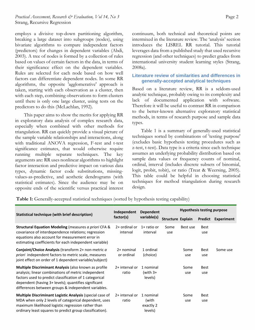
Table 1 is a summary of generally-used statistical techniques sorted by combinations of 'testing purpose' (excludes basic hypothesis testing procedures such as z-test, t-test). Data type is a criteria since each technique assumes an underlying probability distribution based on sample data values or frequency counts of nominal, ordinal, interval (includes discrete subsets of binomial, logit, probit, tobit), or ratio (Treat & Weersing, 2005). This table could be helpful in choosing statistical techniques for method triangulation during research design.

Table 1: Generally-accepted statistical techniques (sorted by hypothesis testing capability) 

 Statistical technique (with brief description)  

Independentfactor(s) 

Dependentvariable(s) 

Hypothesis testing purpose 

Structure Explain  Predict Experiment

Structural Equation Modeling (measures a priori CFA &  covariance of interdependence relations; regression equations also account for measurement error in estimating coefficients for each independent variable) 

2+ ordinal or interval 

1+ ratio or interval 

Some use 

Best use  Best use 

 

Conjoint/Choice Analysis (transform 2+ non‐metric a priori  independent factors to metric scale, measures joint effect on order of 1 dependent variable/subject) 

2+ nominal or ordinal 

1 ordinal (choice) 

  Some use 

Best use 

Some use 

Multiple Discriminant Analysis (also known as profile analysis; linear combinations of metric independent factors used to predict classification of 1 categorical dependent (having 3+ levels); quantifies significant differences between groups & independent variables. 

2+ interval or ratio 

1 nominal (with 3+ levels) 

  Some use 

Best use 

 

Multiple Discriminant Logistic Analysis (special case of MDA when only 2 levels of categorical dependent, uses maximum likelihood logistic regression rather than ordinary least squares to predict group classification). 

2+ interval or ratio 

1 nominal (with 

exactly 2 levels) 

  Some use 

Best use 

 

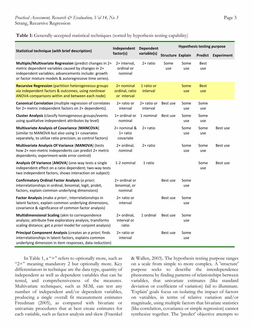
Practical Assessment, Research & Evaluation, Vol 14, No 3 Page 3 Strang, Recursive Regression Table 1: Generally-accepted statistical techniques (sorted by hypothesis testing capability) 

 Statistical technique (with brief description)  

Independentfactor(s) 

Dependentvariable(s) 

Hypothesis testing purpose 

Structure Explain  Predict Experiment

Multiple/Multivariate Regression (predict changes in 2+ metric dependent variables caused by changes in 2+ independent variables; advancements include: growth or factor mixture models & autoregressive time series). 

2+ interval, ordinal or nominal 

2+ ratio  Some use 

Some use 

Best use 

 

Recursive Regression (partition heterogeneous groups via independent factors & outcomes, using nonlinear ANOVA comparisons within and between each node) 

2+ nominal ordinal, ratio or  interval 

1 ratio or interval 

  Some use 

Best use 

 

Canonical Correlation (multiple regression of correlates for 2+ metric independent factors on 2+ dependents). 

2+ ratio or interval 

2+ ratio or interval 

Best use Some use 

Some use 

 

Cluster Analysis (classify homogeneous groups/events using qualitative independent attributes by level) 

1+ ordinal or nominal 

1 nominal  Best use Some use 

Some use 

 

Multivariate Analysis of Covariance [MANCOVA] (similar to MANOVA but also using 1+ covariates separately, to utilize ratio precision, as control factors) 

2+ nominal & 1+ ratio  covariate 

2+ ratio    Some use 

Some use 

Best use 

Multivariate Analysis Of Variance [MANOVA] (tests how 2+ non‐metric independents can predict 2+ metric dependents; experiment‐wide error control) 

2+ ordinal, nominal 

2+ ratio    Some use 

Some use 

Best use 

Analysis Of Variance [ANOVA] (one‐way tests a single independent effect on a ratio dependent; two‐way tests two independent factors, shows interaction on subject) 

1‐2 nominal  1 ratio      Some use 

Best use 

Confirmatory Ordinal Factor Analysis (a priori; interrelationships in ordinal, binomial, logit, probit, factors, explain common underlying dimensions) 

2+ ordinal or binomial, or nominal 

  Best use Some use 

   

Factor Analysis (make a priori ; interrelationships in latent factors, explain common underlying dimensions, covariance & significance of common factor analysis) 

2+ ratio or interval 

  Best use Some use 

   

Multidimensional Scaling (akin to correspondence analysis; attribute free exploratory analysis, transforms scaling distance; get a priori model for conjoint analysis) 

2+ ordinal, interval or 

ratio 

1 ordinal  Best use Some use 

   

Principal Component Analysis (creates an a priori; finds interrelationships in latent factors, explains common underlying dimension in item responses, data reduction)

2+ ratio or interval 

  Best use Some use 

   

In Table 1, a “+” refers to optionally more, such as “2+” meaning mandatory 2 but optionally more. Key differentiators in technique are the data type, quantity of independent as well as dependent variables that can be tested, and comprehensiveness of the measures. Multivariate techniques, such as SEM, can test any number of independent and/or dependent variables, producing a single overall fit measurement estimates Freedman (2005), as compared with bivariate or univariate procedures that at best create estimates for each variable, such as factor analysis and skew (Fraenkel

& Wallen, 2003). The hypothesis testing purpose ranges on a scale from simple to more complex. A 'structure' purpose seeks to describe the interdependence phenomena by finding patterns of relationships between variables, that univariate estimates (like standard deviation or coefficient of variation) fail to illuminate. 'Explain' goals focus on isolating the impact of factors on variables, in terms of relative variation and/or magnitude, using multiple factors that bivariate statistics (like correlation, covariance or simple regression) cannot synthesize together. The 'predict' objective attempts to

Practical Assessment, Research & Evaluation, Vol 14, No 3 Page 4 Strang, Recursive Regression forecast the changes in a key dependent variable by measuring the impact of all known independent factors. 'Experiment' approaches manipulate factors using treatments, while keeping control variables constant and/or using group blocking factors, to isolate and measure impact on a dependent variable (Keppel & Wickens, 2004). Most approaches attempt to capture estimates of unknown error variation (Ullman & Bentler, 2003), at least as a complement of effect size (1 – r2). The table is a summary suggesting 'best use' and 'some use' alternatives, partially informed by Hancock and Samuelsen (2007) as well as Treat and Weersing (2005).

RR comparisons, contrasts and advantages

First, as noted earlier, RR should be used in combination with other techniques for method triangulation. In terms of fit within the generally-accepted statistical methods, RR (as discussed here) can be strategically compared with other exploratory or cause-effect analytic alternatives using the 'hypothesis testing purpose' and 'Predict' column in Table 1. RR can be used for any distribution type since it is a non-parametric statistical technique (Freedman, 2005), but in the literature it is often applied when the normal distribution is hypothesized. One of the most powerful methods for all hypothesis testing purposes is Structural Equation Modeling (SEM), but there are situations when RR is more appropriate. The arguments for using RR instead of SEM are: SEM requires definite covariance measurements (or it will fail), it assumes an underlying normal distribution and attempts to account for unknown error (which can invalidate natural data-driven models). Finally, adjusting parameters in SEM to fit sample measurement data to a structural model can be a tedious process. Conjoint/Choice Analysis is similar to RR in that it measures predictive effect on the individual subject (not group). However, conjoint analysis requires ordinal level input, borrowing on the conditional marginal/joint probability logic - or odds ratio as described by Osborne (2006) - and is best used to measure an a priori choice model (created from multidimensional scaling) that will attempt to predict an ordinal value.

Multiple Discriminant Analysis (MDA) - also called profile analysis in the literature (Ding, 2001) – is similar to RR in that both can use linear combinations of metric independent factors to predict the classification of one categorical dependent variable, itself having three or more levels in the scale. MDA quantifies the significant differences between groups and independent variables, whereas RR quantifies the significant differences

between different individuals, using a different (or the same) predictor at each level, to predict a metric (ratio or interval) outcome. Therefore, RR has more natural behavioral predictive capability, in terms of nonlinear levels of analysis between groups. Additionally, RR has more statistical precision with respect to regressing on a ratio or interval scale as compared with nominal (DeVellis, 1991). Criterion profile analysis is an interesting variation of MDA that is similar (and seems as powerful) as RR, as described by Culpepper (2008) which used ordinal predictors with a covariance function to predict a ratio dependent variable.

Notwithstanding that some authors will describe RR as being hierarchical or non-hierarchical cluster analysis, RR is differentiated here by its use of ratio or interval dependent variables (mainly their underlying normal distributions), and by the use of nonlinear regression to isolate heterogeneous groups, whereas the former is positioned as a structure building technique by identifying homogeneous group classes. Cluster analysis uses variables to identify unobservable similar traits between subjects (or events), producing a simplified typology of homogeneous subgroups. The predictor variables of cluster analysis are categorical (not ratio). A common theme in cluster analysis and RR is they both attempt (like conjoint analysis) to measure outcomes of individual behavior (not average group interrelationships such as SEM and similar multivariate techniques).

Key benefits and limitations of RR

A benefit of RR, akin to SEM, is its aesthetic ability to produce an appealing diagram accompanied by statistical estimates. Most RR software can generate vertical or horizontal decision trees, showing how the factors predict the dependent variable. This RR dendrogram can be used as a top-down decision making chart (explained later). SEM also produces an aesthetically appealing yet useful model of the interrelationships, for a different purpose than RR (structural modeling, not multi-level interaction and prediction).

Notwithstanding the strengths of RR for nonlinear multilevel prediction of a key metric outcome, RR has two major limitations as compared with most of the aforementioned alternatives. One limitation is its lack of an overall multivariate model fit estimate. A second limitation - which is argued here to be a benefit – is that RR lacks an unknown error variance measurement. This last feature should not be confused with the bivariate

Practical Assessment, Research & Evaluation, Vol 14, No 3 Page 5 Strang, Recursive Regression measures that are provided for each node split, since these do measure explained variance (subsequently a complement can be interpolated). The other perspective argued is that natural behavior can be best modeled by assuming unknown variance is part of the model, captured in one or more of the independent factors. This last perspective is what gives RR realism as a dynamic multilevel predictor, driven by the data, not theory.

Finally, RR is not a true multivariate technique because it does not produce a single measurement of fit for all the factors and variables. Instead RR produces a nonlinear road map of how the data unfolds, while borrowing certain robust principles from multivariate techniques such as discriminant analysis, structural equation modeling, factor mixture analysis, as well as the more commonly known analysis of variance. Subsequently, what is missing in RR is an overall comparison of good and bad fit such as SEM provides, using the GFI (good fit) and RMSEA (bad fit). These can be calculated from the estimates but it is a tedious process.

Methodology of applying RR in LISREL RR is described herein as implemented in LISREL,

yet it was also successfully tested with SAS. LISREL RR has the advantage of being more 'plug-and-play' (user friendly) than SAS, in that the former requires little more than factor definitions, whereby SAS requires a complex procedure. Alternative software is available, but LISREL has the benefit of being low-cost, and the student edition is free (version 8r5 and up include RR).

In LISREL, RR can be written as a command script, or a menu-driven interface can be used. The RR module is called Formal Inference-Based Recursive Modeling, and is based on the mathematical work of Hawkins, Young and Rusinko (1997). In general, LISREL RR uses a nonlinear statistical principle, meaning that a significant model can be produced without requiring the dependent variables (y-axis) to have a constant unit change rate (slope) over the independent factors (x-axis). Instead, RR algorithms look for linear relationships within the node group, but often using different independent factors for every group. In fact, this is one of the most powerful benefits of RR in that it can produce a more natural data-driven explanatory model that identifies different predictors when unobservable conditions change (much like latent class models except multiple factors can be used between independent and dependent units on the regression slope). In this sense, RR is multidimensional. A way to explain this is to

consider a linear regression equation that might read: Y=Slope + (Var1 x Beta1); but in RR, conditional logic applies: if Var1=1 ... else if 9, Y=S + (Var1 x Beta9).

ANOVA f-tests are first used to identify significant subgroups based on linear regression of predictors on dependent variable(s), and then by calculating effect size measures. Within each subgroup (node), the strongest predictor of the dependent variable is isolated using t-tests (similar to Marascuilo, Kruskal-Wallis, etc), depending on the data type. Adjustments are made to account for how many factors were tested (post-hoc regression), ensuring the most statistically significant predictor is chosen for each node. In practice, recursive regression can test any independent factor and/or dependent variable as a predictor to partition the data into increasingly smaller groups. Any predictor can be used and reused to split new groups into nodes.

RR algorithms in LISREL

There are two methods for RR in LISREL 8r8: non-parametric categorical and parametric/ non-parametric continuous. The more powerful parametric format of RR (CONFIRM) can compare any type of independent factors (with up to 10 levels) but the dependent variable must be a continuous ratio or interval data type (a typical assumption for normal distributions). Parametric RR typically converts dependent variables into 20 frequency classes before conducting regression. The non-parametric algorithms of RR (CATFIRM) can also process any type of independent factor - nominal, ordinal, interval or ratio data type (up to 10 levels), but the dependent variable must be a nominal which is converted before testing to an interval with a bounded range (using a discrete 1 to 16 scale). Both RR methods are similar in LISREL - each can process up to 1000 predictors with unlimited sample size (DuToit, DuToit & Hawkins, 2001). CONFIRM is discussed from here on, as it is newer and can process ratio as well as interval dependent variables, and it is applied in the tutorial.

There are five types of independent factors available, each with different options, such as missing data flags “?”, conversion masks, along with splitting and merging significance levels. Predictor types affect how the node splitting takes place (such as whether only adjacent nodes can be joined, as with powerful floating type). A common behavior observed is that all predictor scales will range at best from 0 to 9 internally (10 levels). Since predictor definitions are complicated to explain (and testing revealed potential discrepancies with the

Practical Assessment, Research & Evaluation, Vol 14, No 3 Page 6 Strang, Recursive Regression software documentation), a brief tutorial overview is provided. Predictor types are briefly enumerated below:

• character – nominal, only first byte used (if not unique, a new letter is substituted), up to 10 levels;

• free – nominal, one byte, up to 10 levels, direct from data or substituted using a conversion mask;

• monotonic - ordinal, one byte, up to 10 levels, direct from data or substituted using a conversion mask;

• floating – mixed nominal & ordinal (ordinal only for adjacent levels), one byte, same as above;

• real predictor – ratio or interval, will be scaled to 10 levels as a discrete interval.

The statistical principle underlying Formal Inference-Based Recursive Modeling in LISREL “can be described as a piecewise constant model” (Jöreskog, 2006, p 17), an overall nonlinear technique. This means that the slope delta (for changes) between a predictor and the dependent variable can increase, decrease or remain the same, from one unit to the next. Generally though, a smooth unit change rate is assumed (no drastic changes). The RR module in LISREL 8r8 for ratio continuous dependent variables is CONFIRM version 2r3 (RRR). RRR applies the divisive principle, creating nodes by testing all predictors to split groups into successively smaller units. Predictors can change at every node and level, plus they can be reused. There are many customizable options for RRR, allowing a researcher to fine tune parameters such as significance levels for node splitting, and also for merging, minimum node size, etc., but all have reasonable defaults. More of this will be explained in a subsequent section were RRR is applied to analyze an educational study.

It may help to explain a typical RRR algorithm sequence for identifying a predictor to split a node. This begins with the first predictor, calculating descriptive statistics for all records by the unique levels available. For example, if a predictor were culture, with possible values of “E”, “W”, “B”, then the predictor would have three levels, whereby the mean as well as standard deviation would be calculated for each of these (using all applicable records), forming temporary groups of likely unequal sizes. The next step is to determine which if any of these temporary groups could be merged. Pairwise

t-tests are calculated for each combination of two groups, to compare the means and standard deviations (Chi x2 is used in CATFIRM). Starting with the lowest t-test estimate (least different group), the significance level is tested to determine if it is different (can be split, and if so, they are left separate for the time being) or homogeneous (should be merged, and if so, these two groups and levels will be merged). RRR has a mechanism to retest temporary merged nodes (using one of the optional parameters), to protect against poor groupings. Thresholds are also applied, to eliminate groups that have too small a sample size (the default is usually 10 records). The result of this first step is a grouping of the records by one or more of the available scale levels for that single predictor, whereby the more groups that are formed, then the more powerful that particular predictor is, or if only one group remains because all the levels were merged, then obviously the predictor is not significant. Finally, an ANOVA f-test is applied for the predictor (using pooled variances in this case), to compare the analysis of variance explained between groups. This is accompanied by a calculation to produce the Bonferroni significance (modified p-value), along with a more conservative adjusted p-value based on parsimony (degrees of freedom and reflecting number of levels).

The above procedure repeats for all other 'eligible' predictors. The best predictor is selected based on the smallest adjusted p-value. That was the first node split. The whole sequence again repeats using all predictors, for each of the new subgroups created by the node split (thus the sample size for child nodes is continually decreasing). As explained previously, the same or a new predictor can be nominated for adjacent and child nodes. This continues until all significant splits have been selected according to the thresholds (currently the default is 20 nodes), creating terminal nodes. The output consists of a dendrogram (top-down tree diagram) with the most significant predictors (and adjacent node groups) at the top, followed by the next levels of statistically significant predictors; with the terminal child node groups towards the bottom (no more splits below them). Statistical estimate proofs are appended at the bottom of the output (in a structured list format).

The only estimate missing from the RRR detailed output is a predictor as well as overall effect size. However, these can be easily calculated using ANOVA f-tests sum of squares and total squares (the latter includes the standard error residual). The interpretation of the result can rely on Cohen (1992, pp 157-158),

Practical Assessment, Research & Evaluation, Vol 14, No 3 Page 7 Strang, Recursive Regression whereby 0.80 is a large effect, 0.50 corresponds to medium effect, while 0.20 is considered a small effect. One point argued is 0.20 is a significant benchmark for social science research (Keppel & Wickens, 2004, pp 162 & 174-176). Additional fit indices could be added to RRR, offering multivariate analysis of t-test and ANOVA estimates.

One useful capability of RRR is to treat missing data as theoretically significant, by assigning a scale value, such as an “-1” (rather than substituting missing-at-random with similar profiles, imputing using mean functions, or deleting the data row). For example, when processing items on immigration visa applications, treating item non-responses as a scale level is purposeful, because the missing data event can be meaningful.

A powerful dynamic ability of RRR is to allow independent factors to be 'eligible' (included) in the t-test and ANOVA (to capture variance), yet 'prevent' it from actually creating a node split. This might be considered analogous to having covariates included with independent factors in MANCOVA tests of dependent variables.

Analysis and discussion of RRR applied to an educational study

An educational study employed RRR (along with other exploratory methods such as factor analysis and SEM) to analyze the learning style of international university students, across several course subjects, using academic grade as the dependent variable (ratio). As an overview of the Strang (2008a) study, the learning style and culture constructs were first confirmed using ordinal factor analysis, and then sample normality was established using descriptive statistics and univariate tests. RRR was used in combination with factor analysis (FA) and SEM, to uncover hidden nonlinear relationships and interactions that FA and SEM could not isolate. An interesting benefit was that RRR confirmed how insignificant items in the learning style model impacted academic performance, thus identifying exactly where theory improvement was needed (Strang, 2008a).

Independent factors and variables used in RRR tutorial

The Index of Learning Styles (ILS) was the key instrument (Strang, 2008a). ILS (Felder & Soloman, 2001) is a survey with a four dimension model that “classifies students according to where they fit on a number of scales pertaining to the ways they receive and

process information” (Felder & Silverman, 1988, p 674). The 44-item ILS instrument is designed on four dimensions (latent factors), each representing two polarized sub scales: visual-verbal, sensing-intuitive, active-reflective, and sequential-global, as briefly enumerated below.

1. Input - visual (prefer visual representations of material, such as pictures, diagrams, flow charts) or verbal (prefer written and spoken explanations);

2. Perceiving - sensing (concrete, practical, oriented toward facts and procedures) or intuitive (conceptual, innovative, oriented toward theories and underlying meanings);

3. Processing - active (learn by trying things out, enjoy working in groups) or reflective (learn by thinking things through, prefer working alone or 1-2 familiar partners);

4. Understanding - sequential (linear thinking process, learn in incremental steps) or global (holistic thinking process, learn in large leaps); (adapted from: Felder & Spurlin, 2005, pp 104-106).

The original sample size was large and to preserve copyright, the dataset was truncated after the first 500 records to form a mini sample (n=500). Two course subjects are included in this sample, as nominal data types, coded as 'free' in RRR, with masks of: M = management and S = statistics. All of the 44 items measuring the ILS model were coded in RRR as 'float', with a conversion mask to match the first letter of the learning style theory. For example, “A” represents active learning style. Since two “V” codes were possible for the input dimension, “W” was used for verbal (implying its true theoretical meaning). Grade was the dependent variable, coded in RRR as 'continuous' type (labeled 'FinalGPV' meaning Grade Point Value). There were no missing values in the sample data (responses were enforced online), but the substitution capability of RRR was adequately tested by changing codes in the data to more meaningful mnemonics.

Configuration options for RRR example

Most statistical software programs have numerous configuration options for each procedure, and LISREL RRR is no exception. Usually the defaults are appropriate. However, the case study dataset contained numerous binary independent factors which tended to follow a logistic distribution (based on confirmatory

Practical Assessment, Research & Evaluation, Vol 14, No 3 Page 8 Strang, Recursive Regression ordinal factor analysis), and the defaults in LISREL tended to be conservative, allowing for numerous splits, which generated a high volume of estimates. Therefore, the configuration was modified to use more demanding parameters, and those critical changes will be mentioned here (the LISREL script is shown in the appendix). Table 2 lists the RRR runtime configuration and several important predictor definition examples.

Several key parameters from Table 2 will be elaborated upon. The thresholds (#2) was set to 100 observations needed as minimum node size for just analysis (not creation), and maximum (#6) set to 20 node groups for analysis (not creation). These are rigorous threshold parameter settings intended to reduce the amount of output child node levels. Obviously a large sample was expected for the original research design (100 as a minimum node analysis size is

demanding). It should be mentioned that the LISREL authors recommend “the sample size needs to be in three digits before recursive partitioning is likely to be worth trying” (Jöreskog, 2006, p 1), but this refers to the total sample size, not node split analysis size, so parameters #2 and #6 should be adjusted to realistic thresholds since they were set artificially high in this example to reduce the amount of output. The pooled ANOVA mean squares variance (#9) was selected (becomes the denominator of t-test formula), after evaluating the two-group variances approach, because the former reflected all observations (not just two adjacent groups). Pooled variances (used here) is preferred if the data is not heteroscedastic and does not contain outliers, which was obvious in the original study since the items are binary choice responses.

Table 2: RRR parameters invoked with mini sample

.... Note that only certain parameters are shown below to illustrate important features of RRR – see full listing of command script.

.....Below are examples of predictor definitions, all but “InputVar43” are eligible for node splitting, prevented by “1” in column 4. InputVar43 43 0 '1' 1 2 'VW' 0.9 1.0 ! Predictor NOT eligible for node splits, but it WILL be included in ANOVA. UnderstandVar44 44 0 '1' 0 2 'SG' 0.9 1.0 ! This predictor IS eligible to trigger node splits. ClassVar45 45 0 'f' 0 2 'MS' 0.9 1.0 ! This predictor IS eligible to trigger node splits. 1 100 .00100 1.00000 1.00000 20 0 0 1 .0000000 1 0 0 0 0!Parameters: #1 #2 #3 #4 #5 #6 #7 #8 #9 #10 #11 #12 #13 #14 #15 ! #1: '1'=detailed output, #2: minimum group size for splitting analysis = 100, #3: minimum ANOVA SSD % for splitting = 0.001,! #4: t-test significance = 1.0%, #5: conservative node splitting significance = 1.0%, #6: stop merging group after levels = 20, ! #7: external degrees of freedom = 0, !#8: ASCII data file format = 0, #9: '1'=pooled variance, '0'=two group variance, ! #10: external variance % = 0.0, #11: p-values methodology = 1; #12-#15 are not used.

The other important point to highlight is how to prevent a predictor from causing node splits, yet still include the mean and standard deviations in ANOVA analysis, as shown by the “InputVar43” in Table 2. Although this was originally a possible split predictor in the study, it was set ineligible because earlier confirmatory ordinal factor analysis determined this (and other) fields were not reliable. A caveat is the LISREL 8r8 manual and help (reviewed in the study) incorrectly described that setting, so readers should test it first.

Interpreting RRR dendrograms

RRR was applied to the mini sample dataset, and note the interpretation is different compared with the full sample study. The output from RRR is summarized in a thumbnail dendrogram, followed by a detailed yet rudimentary dendrogram (supplemented by a large

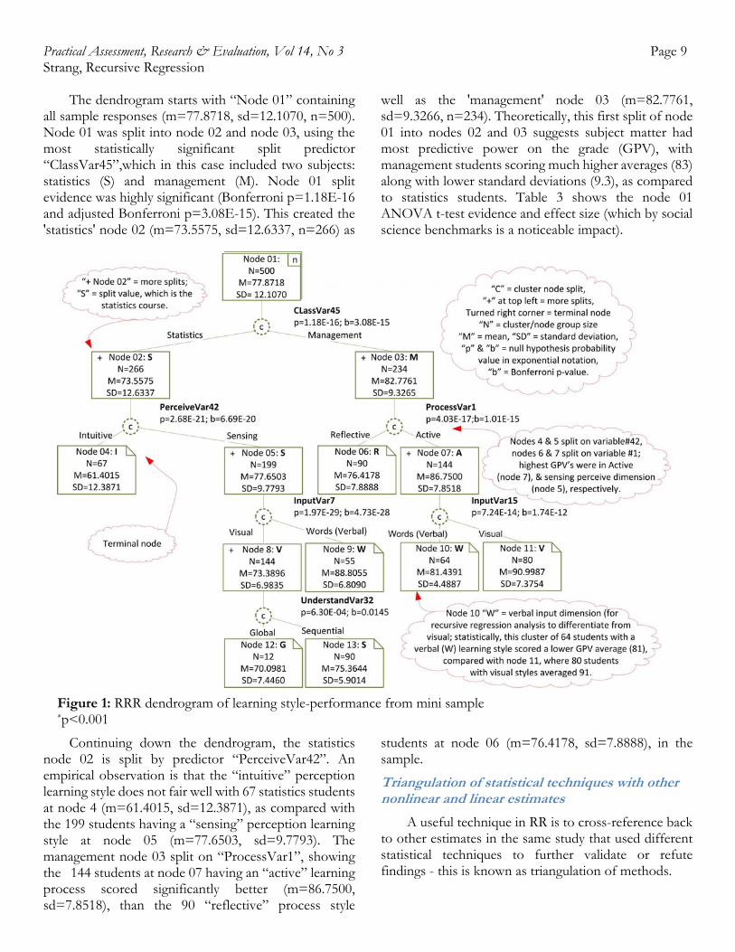
volume of statistical estimates). The dendrogram in Figure 1 was enhanced from the RRR using color, boxes and comments. A few common points can be made on the dendrogram in Figure 1. Each node box lists node group size, mean, and standard deviation. The node splitting used only certain 'eligible' predictors in the data, regressed on GPV, but as noted, the means of ineligible predictors were still included in the ANOVA estimates for split effect size. All results were statistically significant (most at a very high level), otherwise they would not appear in the dendrogram.

The estimates are reproduced without editing of the decimal point for readability, so as to better cross-reference the tables and text with the dendrogram. The theory and codes used in the upcoming dendrogram and analysis are fully explained in the original study by Strang and colleagues (2008a).

Practical Assessment, Research & Evaluation, Vol 14, No 3 Page 9 Strang, Recursive Regression

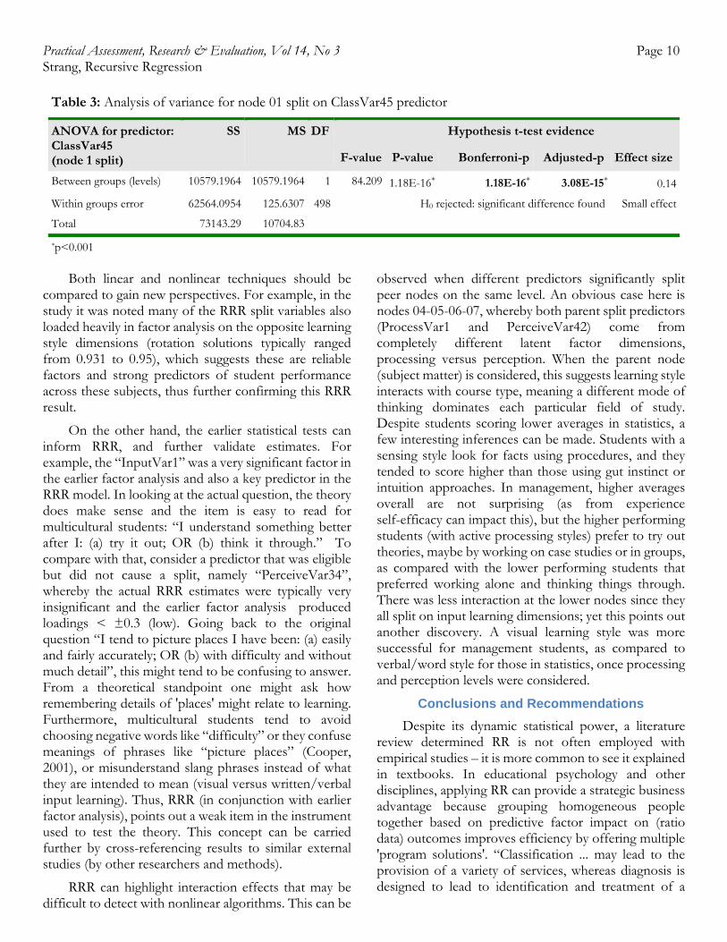
The dendrogram starts with “Node 01” containing all sample responses (m=77.8718, sd=12.1070, n=500). Node 01 was split into node 02 and node 03, using the most statistically significant split predictor “ClassVar45”,which in this case included two subjects: statistics (S) and management (M). Node 01 split evidence was highly significant (Bonferroni p=1.18E-16 and adjusted Bonferroni p=3.08E-15). This created the 'statistics' node 02 (m=73.5575, sd=12.6337, n=266) as

well as the 'management' node 03 (m=82.7761, sd=9.3266, n=234). Theoretically, this first split of node 01 into nodes 02 and 03 suggests subject matter had most predictive power on the grade (GPV), with management students scoring much higher averages (83) along with lower standard deviations (9.3), as compared to statistics students. Table 3 shows the node 01 ANOVA t-test evidence and effect size (which by social science benchmarks is a noticeable impact).

Figure 1: RRR dendrogram of learning style-performance from mini sample *p<0.001

Continuing down the dendrogram, the statistics node 02 is split by predictor “PerceiveVar42”. An empirical observation is that the “intuitive” perception learning style does not fair well with 67 statistics students at node 4 (m=61.4015, sd=12.3871), as compared with the 199 students having a “sensing” perception learning style at node 05 (m=77.6503, sd=9.7793). The management node 03 split on “ProcessVar1”, showing the 144 students at node 07 having an “active” learning process scored significantly better (m=86.7500, sd=7.8518), than the 90 “reflective” process style

students at node 06 (m=76.4178, sd=7.8888), in the sample.

Triangulation of statistical techniques with other nonlinear and linear estimates

A useful technique in RR is to cross-reference back to other estimates in the same study that used different statistical techniques to further validate or refute findings - this is known as triangulation of methods.

Practical Assessment, Research & Evaluation, Vol 14, No 3 Page 10 Strang, Recursive Regression

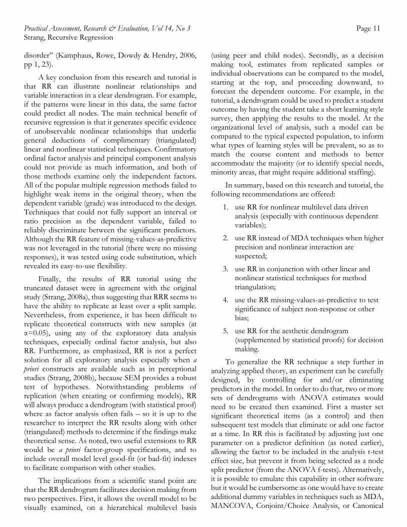
Table 3: Analysis of variance for node 01 split on ClassVar45 predictor

ANOVA for predictor: ClassVar45 (node 1 split)

SS MS DF Hypothesis t-test evidence

F-value P-value Bonferroni-p Adjusted-p Effect size

Between groups (levels) 10579.1964 10579.1964 1 84.209 1.18E-16* 1.18E-16* 3.08E-15* 0.14

Within groups error 62564.0954 125.6307 498 H0 rejected: significant difference found Small effect

Total 73143.29 10704.83

*p<0.001

Both linear and nonlinear techniques should be compared to gain new perspectives. For example, in the study it was noted many of the RRR split variables also loaded heavily in factor analysis on the opposite learning style dimensions (rotation solutions typically ranged from 0.931 to 0.95), which suggests these are reliable factors and strong predictors of student performance across these subjects, thus further confirming this RRR result.

On the other hand, the earlier statistical tests can inform RRR, and further validate estimates. For example, the “InputVar1” was a very significant factor in the earlier factor analysis and also a key predictor in the RRR model. In looking at the actual question, the theory does make sense and the item is easy to read for multicultural students: “I understand something better after I: (a) try it out; OR (b) think it through.” To compare with that, consider a predictor that was eligible but did not cause a split, namely “PerceiveVar34”, whereby the actual RRR estimates were typically very insignificant and the earlier factor analysis produced loadings < ±0.3 (low). Going back to the original question “I tend to picture places I have been: (a) easily and fairly accurately; OR (b) with difficulty and without much detail”, this might tend to be confusing to answer. From a theoretical standpoint one might ask how remembering details of 'places' might relate to learning. Furthermore, multicultural students tend to avoid choosing negative words like “difficulty” or they confuse meanings of phrases like “picture places” (Cooper, 2001), or misunderstand slang phrases instead of what they are intended to mean (visual versus written/verbal input learning). Thus, RRR (in conjunction with earlier factor analysis), points out a weak item in the instrument used to test the theory. This concept can be carried further by cross-referencing results to similar external studies (by other researchers and methods).

RRR can highlight interaction effects that may be difficult to detect with nonlinear algorithms. This can be

observed when different predictors significantly split peer nodes on the same level. An obvious case here is nodes 04-05-06-07, whereby both parent split predictors (ProcessVar1 and PerceiveVar42) come from completely different latent factor dimensions, processing versus perception. When the parent node (subject matter) is considered, this suggests learning style interacts with course type, meaning a different mode of thinking dominates each particular field of study. Despite students scoring lower averages in statistics, a few interesting inferences can be made. Students with a sensing style look for facts using procedures, and they tended to score higher than those using gut instinct or intuition approaches. In management, higher averages overall are not surprising (as from experience self-efficacy can impact this), but the higher performing students (with active processing styles) prefer to try out theories, maybe by working on case studies or in groups, as compared with the lower performing students that preferred working alone and thinking things through. There was less interaction at the lower nodes since they all split on input learning dimensions; yet this points out another discovery. A visual learning style was more successful for management students, as compared to verbal/word style for those in statistics, once processing and perception levels were considered.

Conclusions and Recommendations Despite its dynamic statistical power, a literature

review determined RR is not often employed with empirical studies – it is more common to see it explained in textbooks. In educational psychology and other disciplines, applying RR can provide a strategic business advantage because grouping homogeneous people together based on predictive factor impact on (ratio data) outcomes improves efficiency by offering multiple 'program solutions'. “Classification ... may lead to the provision of a variety of services, whereas diagnosis is designed to lead to identification and treatment of a

Practical Assessment, Research & Evaluation, Vol 14, No 3 Page 11 Strang, Recursive Regression disorder” (Kamphaus, Rowe, Dowdy & Hendry, 2006, pp 1, 23).

A key conclusion from this research and tutorial is that RR can illustrate nonlinear relationships and variable interaction in a clear dendrogram. For example, if the patterns were linear in this data, the same factor could predict all nodes. The main technical benefit of recursive regression is that it generates specific evidence of unobservable nonlinear relationships that underlie general deductions of complimentary (triangulated) linear and nonlinear statistical techniques. Confirmatory ordinal factor analysis and principal component analysis could not provide as much information, and both of those methods examine only the independent factors. All of the popular multiple regression methods failed to highlight weak items in the original theory, when the dependent variable (grade) was introduced to the design. Techniques that could not fully support an interval or ratio precision as the dependent variable, failed to reliably discriminate between the significant predictors. Although the RR feature of missing-values-as-predictive was not leveraged in the tutorial (there were no missing responses), it was tested using code substitution, which revealed its easy-to-use flexibility.

Finally, the results of RR tutorial using the truncated dataset were in agreement with the original study (Strang, 2008a), thus suggesting that RRR seems to have the ability to replicate at least over a split sample. Nevertheless, from experience, it has been difficult to replicate theoretical constructs with new samples (at α=0.05), using any of the exploratory data analysis techniques, especially ordinal factor analysis, but also RR. Furthermore, as emphasized, RR is not a perfect solution for all exploratory analysis especially when a priori constructs are available such as in perceptional studies (Strang, 2008b), because SEM provides a robust test of hypotheses. Notwithstanding problems of replication (when creating or confirming models), RR will always produce a dendrogram (with statistical proof) where as factor analysis often fails – so it is up to the researcher to interpret the RR results along with other (triangulated) methods to determine if the findings make theoretical sense. As noted, two useful extensions to RR would be a priori factor-group specifications, and to include overall model level good-fit (or bad-fit) indexes to facilitate comparison with other studies.

The implications from a scientific stand point are that the RR dendrogram facilitates decision making from two perspectives. First, it allows the overall model to be visually examined, on a hierarchical multilevel basis

(using peer and child nodes). Secondly, as a decision making tool, estimates from replicated samples or individual observations can be compared to the model, starting at the top, and proceeding downward, to forecast the dependent outcome. For example, in the tutorial, a dendrogram could be used to predict a student outcome by having the student take a short learning style survey, then applying the results to the model. At the organizational level of analysis, such a model can be compared to the typical expected population, to inform what types of learning styles will be prevalent, so as to match the course content and methods to better accommodate the majority (or to identify special needs, minority areas, that might require additional staffing).

In summary, based on this research and tutorial, the following recommendations are offered:

1. use RR for nonlinear multilevel data driven analysis (especially with continuous dependent variables);

2. use RR instead of MDA techniques when higher precision and nonlinear interaction are suspected;

3. use RR in conjunction with other linear and nonlinear statistical techniques for method triangulation;

4. use the RR missing-values-as-predictive to test significance of subject non-response or other bias;

5. use RR for the aesthetic dendrogram (supplemented by statistical proofs) for decision making.

To generalize the RR technique a step further in analyzing applied theory, an experiment can be carefully designed, by controlling for and/or eliminating predictors in the model. In order to do that, two or more sets of dendrograms with ANOVA estimates would need to be created then examined. First a master set significant theoretical items (as a control) and then subsequent test models that eliminate or add one factor at a time. In RR this is facilitated by adjusting just one parameter on a predictor definition (as noted earlier), allowing the factor to be included in the analysis t-test effect size, but prevent it from being selected as a node split predictor (from the ANOVA f-tests). Alternatively, it is possible to emulate this capability in other software but it would be cumbersome as one would have to create additional dummy variables in techniques such as MDA, MANCOVA, Conjoint/Choice Analysis, or Canonical

Practical Assessment, Research & Evaluation, Vol 14, No 3 Page 12 Strang, Recursive Regression Correlation. For those interested to experiment with alternative software, the work of Sarle (1994), and the R Project Group (2008), are good starting points, describing how to design and implement RR scripts with SAS. In an effort to extend the practice of RR, the criterion profile analysis research of Culpepper (2008) was replicated by importing his SPSS dataset. Space limitations preclude a full discussion, yet the dendrogram and estimates were revealing, providing decision making priority and typology on the results. It is recommended researchers do likewise: use triangulated (linear and nonlinear) statistical methods like RR to expand perspectives. For researchers whom are interested in trying RR in practice, a link to the sample dataset and command script are given in the appendix.

References Abdi, H. (2003). Multivariate analysis. In M. Lewis-Beck, A.

Bryman & T. Futing (eds.), Encyclopedia of Social Sciences: Research Methods. Thousand Oaks, CA: Sage.

Cohen, J. (1992). Statistics a power primer. Psychology Bulletin 112: 115-159.

Cooper, T.C. (2001). Foreign language teaching style and personality. Foreign Language Annals, 34 (4), 301-312.

DeVellis, R.F. (1991). Scale development: Theory and application. Newbury Park, CA: Sage.

Culpepper, S.A. (2008). Conducting external profile analysis with multiple regression. Practical Assessment, Research & Evaluation, 13(1). Retrieved 4 March 2008 from: http://pareonline.net/getvn.asp?v=13&n=1

Ding, C.S. (2001). Profile analysis: Multidimensional scaling approach. Practical Assessment, Research & Evaluation, 7(16). Retrieved 15 May 2008 from: http://pareonline.net/getvn.asp?v=7&n=16

DuToit, M.; DuToit, S. & Hawkins, D.M. (2001). Interactive LISREL: User guide. Lincolnwood, IL: Scientific Software International.

Felder, R.M. & Silverman, L.K. (1988). Learning and teaching styles in engineering education. Engineering Education, 78(7), 674-681.

Felder, R.M. & Soloman, B.A. (2001). Index of Learning Styles questionnaire; scoring sheet; learning styles and strategies. North Carolina State University. Retrieved 11 June 2007 from: http://www.ncsu.edu/felder-public/ILSpage.html

Felder, R.M. & Spurlin, J. (2005). Applications, reliability and validity of the index of learning styles. International Journal of Engineering Education 21(1), 103-112.

Fraenkel, J.R. & Wallen, N.E. (2003). How to design and evaluate research in education (5th ed.). New York: McGraw-Hill.

Freedman, DA. (2005). Statistical models for causation: A critical review. In Encyclopedia of Statistics in Behavioral Science. NY: Wiley.

Hancock, G.R. & Samuelsen, K.M. (2007). Advances in latent variable mixture models. Greenwich, CT: Information Age Publishing, Inc.

Hawkins, D.M.; Young, S.S. & Rusinko, A. (1997). Analysis of a large structure-activity data set using recursive partitioning. Quantitative Relationships, 3(7), 101-126.

Jöreskog, K.G. (2006). Formal Inference-Based Recursive Modeling [LISREL]. Hillsdale, NJ: Lawrence Erlbaum Associates.

Kamphaus, R.W.; Rowe, E.W.; Dowdy, E.T. & Hendry, C.N. (2006). Psychodiagnostic assessment of children: Dimensional and categorical approaches. New York: Wiley.

Keppel, G. & Wickens, T.D. (2004). Design and analysis: A researcher's handbook (4th ed.). Upper Saddle River, NJ: Pearson.

McLachlan, P. (1992). Discriminant analysis and pattern recognition. New York: Wiley.

Osborne, J. (2006). Bringing balance and technical accuracy to reporting odds ratios and the results of logistic regression analyses. Practical Assessment Research & Evaluation, 11(7). Retrieved 1 May 2008 from: http://pareonline.net/getvn.asp?v=11&n=7

R Project Group. (2004). Implementing Recursive Regression in SAS. Retrieved 9 June 2006 from: http://www.r-project.org/

Sarle, W. (1994, June 28). Logistic vs discriminant [nonlinear logistic regression in SAS; see also: www.sas.com]. Retrieved 1 May 2004 from: http://lists.mcgill.ca/scripts/wa.exe?A2=ind9406&L=stat-l&D=0&T=0&P=45690

Strang, K.D. (2008a). Quantitative online student profiling to forecast academic outcome from learning styles using dendrogram decision models. Multicultural Education & Technology Journal, 2(4), 215-244.

Strang, K.D. (2008b). Collaborative synergy and leadership in e-business. In J. Salmons & L. Wilson (eds.), Handbook of Research on Electronic Collaboration and Organizational Synergy; PA: IGI Global.

Treat, T.A. & Weersing, B. (2005). Clinical psychology. In Encyclopedia of Statistics in Behavioral Science. NY: Wiley.

Ullman, J.B. & Bentler, P.M. (2003). Structural equation modeling. In I.B. Weiner, J.A. Schinka & W.F. Velicer (Eds.) Handbook of Psychology: Research Methods in Psychology (Vol. 2) NY: Wiley.

Practical Assessment, Research & Evaluation, Vol 14, No 3 Page 13 Strang, Recursive Regression

Appendix

Below are links to the RRR command script and mini sample dataset. To try this, copy both of these files into the same directory (note: both files must have the same name and with exactly the extension as given here). Run LISREL, use the 'file open' menu option, and then enter the complete script filename and extension. Click on the menu option to run the 'Prelis' module, and the results should appear after a few minutes on most computers.

RRR LISREL PRELIS script: http://pareonline.net/sup/v14n3/InterpretingRecursiveRegression.pr2

RRR mini sample ASCII dataset (n=500): http://pareonline.net/sup/v14n3/InterpretingRecursiveRegression.dat

Citation

Strang, Kenneth David (2009). Using recursive regression to explore nonlinear relationships and interactions: A tutorial applied to a multicultural education study. Practical Assessment, Research & Evaluation, 14(3). Available online: http://pareonline.net/getvn.asp?v=14&n=3.

Corresponding Author

Kenneth David Strang University of Technology, Sydney Faculty of Business, School of Marketing Haymarket Plaza, Sydney, NSW 2000, Australia email: kenneth.strang [at] uts.edu.au or KennethStrang [at] aim.com

Author Biography

Dr Strang has a Professional Doctorate in Project Management (high distinction, with concentration in professional adult learning) from RMIT University. He has an MBA (honors) and BS (honors) both from Birmingham University. He is certified as a Project Management Professional® from the Project Management Institute, and is a Fellow of the Life Management Institute (with distinction, specialized in actuary statistics and pension systems), from the Life Office Management Association. His research interests include: transformational leadership, multicultural e-learning, knowledge management, and e-business. His application of these topics are mainly empirical studies and quasi-experiments. He designs and teaches online MBA courses for universities in North America. He teaches multi-disciplinary subjects in business, informatics and education design at University of Technology and Central Queensland University (Australia). He chairs the Learning-in-Business Center at Andragogy International. He supervises PHD and doctorate students.