Using RapidEye and MODIS Data Fusion to Monitor … · Remote Sens. 2015, 7 6511 Heterogeneous...
25
Remote Sens. 2015, 7, 6510-6534; doi:10.3390/rs70606510 remote sensing ISSN 2072-4292 www.mdpi.com/journal/remotesensing Article Using RapidEye and MODIS Data Fusion to Monitor Vegetation Dynamics in Semi-Arid Rangelands in South Africa Andreas Tewes 1,2, *, Frank Thonfeld 1,3 , Michael Schmidt 4 , Roelof J. Oomen 2 , Xiaolin Zhu 5 , Olena Dubovyk 1 , Gunter Menz 1,3 and Jürgen Schellberg 1,2 1 Center for Remote Sensing of Land Surfaces, University of Bonn, Walter-Flex-Str. 3, 53113 Bonn, Germany; E-Mails: [email protected] (F.T.); [email protected] (O.D.); [email protected] (G.M.); [email protected] (J.S.) 2 Institute of Crop Science and Resource Conservation (INRES), University of Bonn, Katzenburgweg 5, 53115 Bonn, Germany; E-Mail: [email protected] 3 Remote Sensing Research Group, Department of Geography, University of Bonn, Meckenheimer Allee 166, 53115 Bonn, Germany 4 Remote Sensing Centre, Environment and Resource Sciences, Department of Science, Information Technology, Innovation and the Arts, GPO Box 5078, Brisbane, Queensland 4001, Australia; E-Mail: [email protected] 5 Ecosystem Science and Sustainability, Colorado State University, NESB 108, 1499 Campus Delivery, Fort Collins, CO 805239, USA; E-Mail: [email protected] * Author to whom correspondence should be addressed; E-Mail: [email protected]; Tel.: +49-228-732-044; Fax: +49-228-732-870. Academic Editors: Clement Atzberger and Prasad S. Thenkabail Received: 2 September 2014 / Accepted: 7 April 2015 / Published: 26 May 2015 Abstract: Image time series of high temporal and spatial resolution capture land surface dynamics of heterogeneous landscapes. We applied the ESTARFM (Enhanced Spatial and Temporal Adaptive Reflectance Fusion Model) algorithm to multi-spectral images covering two semi-arid heterogeneous rangeland study sites located in South Africa. MODIS 250 m resolution and RapidEye 5 m resolution images were fused to produce synthetic RapidEye images, from June 2011 to July 2012. We evaluated the performance of the algorithm by comparing predicted surface reflectance values to real RapidEye images. Our results show that ESTARFM predictions are accurate, with a coefficient of determination for the red band 0.80 < R 2 < 0.92, and for the near-infrared band 0.83 < R 2 < 0.93, a mean relative bias between 6% and 12% for the red band and 4% to 9% in the near-infrared band. OPEN ACCESS
Transcript of Using RapidEye and MODIS Data Fusion to Monitor … · Remote Sens. 2015, 7 6511 Heterogeneous...

Remote Sens. 2015, 7, 6510-6534; doi:10.3390/rs70606510
remote sensing ISSN 2072-4292
www.mdpi.com/journal/remotesensing
Article
Using RapidEye and MODIS Data Fusion to Monitor
Vegetation Dynamics in Semi-Arid Rangelands in South Africa
Andreas Tewes 1,2,*, Frank Thonfeld 1,3, Michael Schmidt 4, Roelof J. Oomen 2, Xiaolin Zhu 5,
Olena Dubovyk 1, Gunter Menz 1,3 and Jürgen Schellberg 1,2
1 Center for Remote Sensing of Land Surfaces, University of Bonn, Walter-Flex-Str. 3, 53113 Bonn,
Germany; E-Mails: [email protected] (F.T.); [email protected] (O.D.);
[email protected] (G.M.); [email protected] (J.S.) 2 Institute of Crop Science and Resource Conservation (INRES), University of Bonn,
Katzenburgweg 5, 53115 Bonn, Germany; E-Mail: [email protected] 3 Remote Sensing Research Group, Department of Geography, University of Bonn, Meckenheimer
Allee 166, 53115 Bonn, Germany 4 Remote Sensing Centre, Environment and Resource Sciences, Department of Science, Information
Technology, Innovation and the Arts, GPO Box 5078, Brisbane, Queensland 4001, Australia;
E-Mail: [email protected] 5 Ecosystem Science and Sustainability, Colorado State University, NESB 108, 1499 Campus
Delivery, Fort Collins, CO 805239, USA; E-Mail: [email protected]
* Author to whom correspondence should be addressed; E-Mail: [email protected];
Tel.: +49-228-732-044; Fax: +49-228-732-870.
Academic Editors: Clement Atzberger and Prasad S. Thenkabail
Received: 2 September 2014 / Accepted: 7 April 2015 / Published: 26 May 2015
Abstract: Image time series of high temporal and spatial resolution capture land surface
dynamics of heterogeneous landscapes. We applied the ESTARFM (Enhanced Spatial and
Temporal Adaptive Reflectance Fusion Model) algorithm to multi-spectral images covering
two semi-arid heterogeneous rangeland study sites located in South Africa. MODIS 250 m
resolution and RapidEye 5 m resolution images were fused to produce synthetic RapidEye
images, from June 2011 to July 2012. We evaluated the performance of the algorithm by
comparing predicted surface reflectance values to real RapidEye images. Our results show
that ESTARFM predictions are accurate, with a coefficient of determination for the red band
0.80 < R2 < 0.92, and for the near-infrared band 0.83 < R2 < 0.93, a mean relative bias
between 6% and 12% for the red band and 4% to 9% in the near-infrared band.
OPEN ACCESS

Remote Sens. 2015, 7 6511
Heterogeneous vegetation at sub-MODIS resolution is captured adequately: A comparison
of NDVI time series derived from RapidEye and ESTARFM data shows that the
characteristic phenological dynamics of different vegetation types are reproduced well.
We conclude that the ESTARFM algorithm allows us to produce synthetic remote sensing
images at high spatial combined with high temporal resolution and so provides valuable
information on vegetation dynamics in semi-arid, heterogeneous rangeland landscapes.
Keywords: RapidEye; MODIS; ESTARFM; image fusion; data blending; vegetation
dynamics; high spatial and temporal resolution; time series
1. Introduction
Time series of vegetation indices derived from remotely sensed data are readily used to monitor
spatial and temporal dynamics of biophysical variables such as Leaf Area Index (LAI) or fraction of
absorbed photosynthetically active radiation (fAPAR) [1,2], and phenological metrics such as day of
green-up and duration of greenness [3]. Multi-temporal measurements of those variables provide
information for spatially distributed environmental modelling across different scales, e.g., for yield
forecasts, ecohydrologic cycles or land cover change [4].
Ecological studies often rely solely on field data, whose collection is time-consuming, cost-intensive
and often limited in space and time. Remote sensing data play a supporting role, but only match poorly
with small scale field measurements due to discrepancies in spatial resolution between the images and
field data [5]. Furthermore, in-field ground truth measurements are hard to compare to remotely sensed
data. Relevant processes may display a small-scale heterogeneity (e.g., spatially varying grazing intensities
or heterogeneous abiotic site conditions [6]) that a selective sampling of species may not capture.
Remotely sensed data exhibiting both high temporal and high spatial resolution show great promise for the
exploration of processes taking place rapidly at scales similar to that of field assessments. Such data are
available from different sensors like IKONOS, Quickbird, RapidEye or SPOT at over-flight intervals from
1 to 5 days. However, these data are costly and may have disadvantages for mapping on medium to large
scales due to a small image footprint or limited spectral resolution [7]. A variety of studies have instead
relied on using the mid-resolution Landsat sensors. For all optical satellites, the continuous temporal
data coverage can be interrupted by clouds, cloud shadows, haze or smoke from fires [7,8].
The above-mentioned factors limit the use of remotely sensed data for detection of rapid surface changes,
including spatial and temporal changes in vegetated surfaces [9]. Medium to low spatial resolution
instruments such as MODIS, SPOT-Vegetation and AVHRR cover the earth on a daily basis over a wide
field of view. This frequency is suitable for monitoring land cover dynamics at large scales [10].
Spatial resolution ranges from 250 m to 1000 m, which is however not satisfactory for tracking changes
(such as vegetation dynamics) and spatio-temporal patterns at ecologically relevant resolutions,
especially in heterogeneous landscapes [11,12].
Fusion of remotely sensed data from different sensors with different spatial and temporal
characteristics is an efficient solution to enhance the capability of remote sensing for the monitoring of
land surface dynamics at varying scales [12,13]. Pohl and Van Genderen [14] define image fusion as

Remote Sens. 2015, 7 6512
“the combination of two or more different images to form a new image by using a certain algorithm”. It
promotionally blends multiple registered images having disparate and distinct yet complementary
attributes. Image fusion aims at enhancing information included in the images and at improving
reliability of the prediction. The outcome mitigates or exceeds the limitations of each dataset used as
input [10,14]. The result may be a combined time series that exhibits both a high temporal and high
spatial resolution [8]. There are numerous scientific papers suggesting the fusion of data from multiple
sensors to provide both high spatial and high temporal resolution [4,15]. However, only few studies
suggest techniques that compute calibrated outputs of spectral radiance or reflectance values, which is
required to study vegetation dynamics or quantitative changes in reflectance over time [9,11].
Gao et al. [9] developed STARFM (Spatial and Temporal Adaptive Reflectance Fusion Model) to
combine the spatial resolution of Landsat imagery with the temporal resolution of coarse-resolution
sensors. A synthetic surface reflectance product at Landsat spatial resolution and high temporal
resolution is obtained by combining spatial information from Landsat imagery and temporal
information from coarse-resolution imagery. STARFM achieves good results if non-mixed
coarse-resolution pixels exist in the area of application (i.e., homogeneous, large land cover patches).
However, performance deteriorates in complex mixtures of small patched land cover types such as
small-scale agriculture [9]. Several studies successfully tested the fusion of Landsat and MODIS in
different environments [8,10,11,16–19].
Zhu et al. [12] developed the ESTARFM (Enhanced Spatial and Temporal Reflectance Fusion Model)
algorithm to improve this shortcoming of the original STARFM method, by using the observed
reflectance trend between two points in time, combined with the spectral unmixing theory [20] to better
predict reflectance in changing, heterogeneous landscapes. Results show that ESTARFM is capable of
preserving spatial details better than STARFM. Emelyanova et al. [17] evaluated the performance of
blending algorithms including STARFM and ESTARFM and found that ESTARFM performed better
where/when spatial variance was dominant, whereas STARFM performed better under prevailing
conditions of temporal variance.
Our motivation for this study was to find a method that overcomes the low temporal resolution of
time series and yet yields high spatial resolution that enables to capture spatial heterogeneity in
vegetation dynamics. To achieve this we used an image fusion algorithm that blends high spatial
resolution RapidEye data and high temporal resolution MODIS data. ESTARFM was selected as the
algorithm of choice because (1) it explicitly improves the fusion accuracy of images especially in
heterogeneous landscapes, and preserves spatial details, (2) it can be used for sensors other than Landsat
and MODIS, (3) it does not require ancillary land cover data, and (4) it is freely available [12,17]. We
are not aware of any study on the fusion of RapidEye with a coarse-resolution sensor. The research
questions underlying this study are:
1. Is the ESTARFM algorithm applicable for generating time series using the combination of
RapidEye and MODIS?
2. Is a time series combining real RapidEye with ESTARFM-computed synthetic images appropriate
for detecting highly dynamic vegetation changes at different small scale bush density classes in
semi-arid rangelands in South Africa?

Remote Sens. 2015, 7 6513
2. Material and Methods
2.1. The Study Area
The study area is situated in the Northern Cape Province of South Africa and lies within the southern
outreaches of the Kalahari (Figure 1). The landscape is a savannah biome, which covers about 1/3 of
South Africa, including most of the far-northern part of the Northern Cape Province [21].
Vegetation cover comprises a woody layer of mainly seasonally deciduous trees and shrubs, especially various
species of the genus Acacia, and a ground layer of annual and perennial grasses and some forbs [22,23].
The study area lies within the southern African summer rainfall zone (October–April). Winters are dry,
with little to no precipitation. Mean annual precipitation is 423 mm with a coefficient of variation of 34%
(calculated over 37 years). Low precipitation has favoured the use of land for pasture farming, since much of
the land is unsuitable for crop cultivation [23]. Rainfall, fire and grazing are the three key driving forces for
vegetation dynamics in the Kalahari ecosystem, as in many other semi-arid rangelands [22,24]. During the
study time period, the area received 203 mm of precipitation (54% less than the long-term average).
Figure 1. Location of study area. Subsets are indicated by black frames. The RapidEye
image (true-colour RGB image using bands 3, 2 and 1) was acquired on 16 November 2011.
Distinctive landmarks visible in the western part are sand dunes stretching from northwest
to southeast and the Gamogara riverbed stretching from south to north. The eastern part
shows the riverbed of Kuruman river stretching from west to east, and foothills of the
Kuruman mountains stretching from southeast to northwest.

Remote Sens. 2015, 7 6514
2.2. Data
2.2.1. The RapidEye Data
The RapidEye system consists of 5 identical satellites placed in a single orbit. Each satellite carries a
5 band multi-spectral optical imager that captures radiation in the blue, green, red, red edge and
near-infrared (NIR) spectral range. At nadir, ground sampling distance is 6.5 m and 5 m after
orthorectification and resampling, respectively [25,26].
Twenty-three RapidEye images were used for our study. They were captured within the time period
June 2011 to July 2012 (covering an entire vegetation growth cycle); with each scene not exceeding a
cloud cover of 20%. Eight images cover the study area in its entirety or for the most part, 15 images just
partially (either eastern or western part of the study area). We formed 2 subsets for ESTARFM input to
reduce data load and shorten image calculation routines. The western subset with an extent of 24 km by
24 km will be referred to as Subset 1, the eastern subset with an extent of 35 km by 24.5 km as Subset 2.
Their respective location is indicated as black frames in Figure 1. The RapidEye images were
orthorectified and atmospherically corrected using the automated processing chain CATENA developed
and maintained by the German Aerospace Center [27]. CATENA relies on the physical model
implemented in the ATCOR software to eliminate atmospheric effects [28]. Clouds in RapidEye images
were masked manually. Areas affected were assigned no-data values and excluded from further analysis.
Table 1 shows that RapidEye and MODIS have corresponding spectral bands, except for RapidEye’s
Red Edge band at 690–730 nm. The study area is crossed by both sensors within a narrow time frame
(RapidEye: 9:25 am–9:45 am GMT, MODIS on Terra: 7:30 am–9:30 am GMT). Both instruments
provide 12 bit radiometric sensitivity. RapidEye products are delivered with 16 bit unsigned integer bit
depth, MODIS with 16 bit signed integer bit depth.
Table 1. RapidEye and MODIS band characteristics.
Band Name Band No Spectral Range [nm]
RapidEye MODIS RapidEye MODIS
Blue 1 3 440–510 459–479
Green 2 4 520–590 545–565
Red 3 1 630–685 620–670
Red Edge 4 - 690–730 -
NIR 5 2 760–850 841–876
2.2.2. The MODIS Data
To minimize the spatial resolution and acquisition time differences between the MODIS and
RapidEye data, we selected the MOD09Q1 product. This product provides surface spectral reflectance
as it would be measured at ground level in the absence of atmospheric scattering or absorption.
It comprises bands 1 and 2 (red and NIR) on the Terra satellite at a 250 m resolution in an 8-day
composite product, where each pixel contains the best possible observation during an 8-day period as
selected on the basis of high observation coverage, low view angle, absence of clouds or cloud shadows,
and aerosol loading ([29]). Additionally, each dataset contains a quality band that was used to assess the

Remote Sens. 2015, 7 6515
quality of each pixel. Higher likeliness to encounter cloud-free pixels and a reasonable trade-off between
workload and temporal resolution of fused products were the reasons why we chose the 8-day composite
product for our study. Missing MOD09Q1 data was substituted by the product MOD09GQ, which provides
bands 1 and 2 at 250 m resolution in a daily gridded product. For visualization purposes, band 4 (green
spectrum) was extracted from the MODIS product MOD09A1. This product is computed at the same
dates as MOD09Q1 and provides bands 1 to 7 at 500 m resolution in an 8-day gridded product. The
MOD09A1 product contains the same observations as MOD09Q1 in band 1 and 2 (according to
Gao et al. [9], pixels are aggregated to 500 m resolution), respectively. By checking the quality band of
every MODIS product, we found that all MODIS images were provided at best quality. To reduce
algorithm computing time, sensor bands not suitable for the purpose of this study were excluded from
the datasets. Accordingly, only red and NIR bands were included for NDVI calculation (for MODIS
input either from MOD09Q1 or MOD09GQ), plus the green band. The MODIS data were re-projected
to the UTM Zone 34 South using the USGS LP DAAC’s MODIS Reprojection Tool Web Interface
(MRTWeb) (https://mrtweb.cr.usgs.gov/). The implementation of ESTARFM requires MODIS data to
be resampled to RapidEye 5 m resolution. No further processing was applied since the MODIS scenes
were provided pre-corrected for atmospheric scattering and absorption. Co-registration of MODIS and
RapidEye images was challenging because differences in spatial resolution were too large as to find
reliable ground control points (GCPs). Visual inspection of 10 randomly selected MODIS and RapidEye
images indicated a good overlay of distinguished landmarks, with none of the MODIS images requiring
manual adjustment.
2.3. The ESTARFM Algorithm
The ESTARFM algorithm requires 2 pairs of fine-resolution and coarse-resolution images as input,
with each pair (t1 and t2) captured at the same date. For the desired prediction date tp, 1 coarse-resolution
image is required. ESTARFM yields a synthetic image at the prediction date tp with the same spatial
resolution as the fine-resolution input images [12].
During the ESTARFM computation, four major steps take place: (1) Two fine-resolution images are
used to search for pixels similar to the central pixel in a moving search window, (2) the spectral and
spatial distance between each similar pixel and the predicted pixel are used to calculate weights of each
similar pixel wi, (3) a linear regression of the coarse-resolution values in the two observed pairs (t1 and t2)
against the fine-resolution values of the similar pixel is used to determine the conversion coefficient vi,
which is then used to convert the change found from the coarse-resolution images to the fine resolution
images, and (4) fine-resolution reflectance from coarse-resolution image at prediction date tp, predicted as:
𝐹(𝑥, 𝑦, 𝑡𝑝) = 𝐹(𝑥, 𝑦, 𝑡0) +∑𝑤𝑖 × 𝑣𝑖 × (𝐶(𝑥𝑖
𝑁
𝑖=1
, 𝑦𝑖 , 𝑡𝑝) − 𝐶(𝑥𝑖 , 𝑦𝑖 , 𝑡𝑜)) (1)
Here, F and C represent fine-resolution image and coarse-resolution image reflectance, (x,y) the
location of the predicted pixel value while xi and yi is the location of ith similar pixel, and t0 is the date
of 1 input pair (t1 or t2). N is the total number of similar pixels of the predicted pixel within a moving
window. The algorithm is explained in detail in Zhu et al. [12].

Remote Sens. 2015, 7 6516
2.4. ESTARFM Implementation
Synthetic images at RapidEye resolution were computed for both subsets using 14 RapidEye scenes
captured between 28 June 2011 and 18 July 2012 as input (with 6 scenes covering both subsets and
4 composites each consisting of two scenes acquired within a short period of time, covering either
subset), combined with the corresponding MODIS images acquired at the closest possible date (i.e.,
forming 10 image pairs; see Figure 2). The MOD09A1 day of the year layer was used to determine the
acquisition day of the majority of pixels, aiming at minimizing the time difference between the MODIS
and RapidEye observations. For image pair formation, 3 MODIS MOD09Q1 products were not available
in 2012 (10 February 2012, 14 April 2012 and 11 July 2012); the daily surface reflectance product
MOD09GQ was used instead. Here, the same acquisition date as of the corresponding RapidEye image
was chosen. Coarse-resolution information at prediction dates (tp) was provided by 39 (Subset 1) and 38
(Subset 2) MODIS images within the time period 04 July 2011 until 03 July 2012, respectively. For
prediction, 3 missing MOD09Q1 datasets in 2012 (02 February 2012, 05 March 2012 and 21 March
2012) were substituted by MOD09GQ products. We chose the MODIS scene dated 14 April 2012 to
only form an image pair with the RapidEye scene dated 19 April 2012 covering Subset 1, but not with
the RapidEye scene acquired on 22 April 2012 (covering Subset 2) due to the major time lag. For this
formation, we chose the MOD09GQ product of the same date instead and simultaneously used the scene
for reflectance prediction of Subset 1. The outcome of this is the different number of prediction dates. The
second image pair (i.e., at date t2) continuously served as first image pair in the next computation step (i.e.,
at date t1). Two temporally closest image pairs were always provided as bracketing images for ESTARFM
prediction. The size of the moving window was set to the size of one MODIS pixel, i.e., corresponding to
50 × 50 RapidEye pixels.
2.5. Accuracy Assessment of ESTARFM Images
The validation of the accuracy of the synthetic images was undertaken using a set of images
independent from those that were used as ESTARFM input. Nine RapidEye scenes, each captured at a
date bracketed by two consecutive RapidEye images used for ESTARFM processing, were used to
compare pixel values in the predicted image with the corresponding pixels in the reference RapidEye
image, on a band by band basis (following Walker et al. [10]). White and light grey coloured acquisition
dates in Figure 2 indicate the image pairs used for cross-comparison. Prediction quality was assessed for
the entire sub-scenes, independent from land cover type or vegetation cover. This yielded a sample size of
24 million to 34 million pixels per image pair, depending on extent and cloud cover. Only one RapidEye
image (captured on 17 January 2012) covered the study area completely, the others either Subset 1 or
Subset 2. The accuracy assessment of our study was based on a scheme proposed by Wald et al. [30] and
Thomas and Wald [31]. We employed the following quantitative criteria:
1. The bias as well as its value relative to the mean value of the observed image should ideally be 0.
The bias is the difference between the mean value of the observed RapidEye and predicted
ESTARFM image.
Remote Sens. 2015, 7 6517
2. The standard deviation of the difference image in relative value, i.e., divided by the mean of the
reference image, should ideally be 0. This measure indicates the level of error at any pixel,
throughout the entire image (thus hereafter referred to as per-pixel level of error).
3. On a band by band basis, the coefficient of determination (R2) between the observed RapidEye
and the synthetic ESTARFM image should be as close as possible to 1. This measures the
pixel-wise similarity in the observed versus the predicted image.
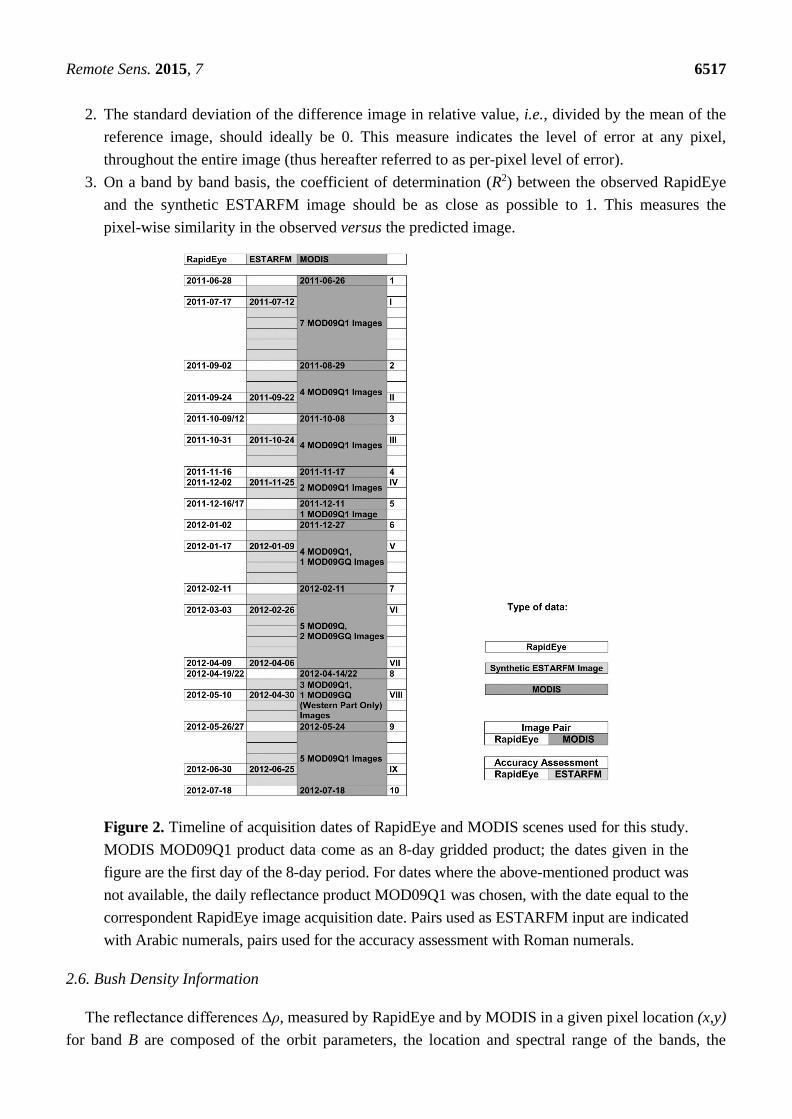
Figure 2. Timeline of acquisition dates of RapidEye and MODIS scenes used for this study.
MODIS MOD09Q1 product data come as an 8-day gridded product; the dates given in the
figure are the first day of the 8-day period. For dates where the above-mentioned product was
not available, the daily reflectance product MOD09Q1 was chosen, with the date equal to the
correspondent RapidEye image acquisition date. Pairs used as ESTARFM input are indicated
with Arabic numerals, pairs used for the accuracy assessment with Roman numerals.
2.6. Bush Density Information
The reflectance differences Δρ, measured by RapidEye and by MODIS in a given pixel location (x,y)
for band B are composed of the orbit parameters, the location and spectral range of the bands, the

Remote Sens. 2015, 7 6518
acquisition time (implying different sun illumination angles), the different atmospheric correction
approaches, the viewing angles, the overlay (co-registration of images) and the spatial resolution of the
sensor, resulting in pixels that are composed of a variety of reflectances. While it is difficult to investigate
the influence of the separate components, the factor of spatial resolution may be analysed based on the
following thoughts: One MODIS pixel exhibiting a spatial resolution of 250 m contains the average
reflectance of all land cover types contained therein, whereas the RapidEye sensor is capable of
dissolving these into 2500 different values (50 × 50 RapidEye pixels, perfect overlay given). Such high
spatial resolution allows for better vegetation classification, and so determines the proportions of land
cover each MODIS pixel is composed of. One basis for vegetation classification is the temporal behaviour
of composited NDVI (Normalized Difference Vegetation Index) time series. Vegetation phenology shows
distinct seasonal patterns in semi-arid savannahs since growth is water-limited [32]. This applies for both
the bush and grass layer. According to Scholes and Walker [33], trees and bushes in southern African
savannahs exhibit signs of growth before the first “effective” rainfall due to their ability to access
subsurface moisture, whereas grasses respond to rainfall events and exhibit a shorter, more intensive
growth pulse.
The widely utilized unsupervised k-means cluster algorithm was used to classify the composited
NDVI time series, derived from 15 (Subset 1) and 16 (Subset 2) RapidEye images used within our study
(i.e., comprising RapidEye images used for algorithm input and for accuracy assessment). Large areas
not used as rangeland were masked and excluded from the classification and further study.
Clusters found by the algorithm were identified using expert knowledge and the above mentioned
orthophotos, and subsequently merged into the user-defined vegetation type classes “grass cover” or
“bush cover” or the type “asphalt, bare soil, non-dynamic surface” for non-vegetated areas. We then
calculated the percentage area classified as “bush cover” falling into each MODIS pixel at 250 m
resolution. Those areas at MODIS pixel resolution that intersected with the class “asphalt, bare soil,
non-dynamic surface” were excluded to reduce the error of interfering signals. On a band by band basis,
the coefficient of determination R² between the observed RapidEye and predicted ESTARFM images was
calculated for every bush density class, thereby determining the prediction accuracy at sub-MODIS scale.
2.7. Monitoring Vegetation Dynamics
Despite its appearance to be a poor indicator of vegetation biomass for low ground cover, a number
of studies confirm the usefulness of NDVI for monitoring vegetation dynamics in arid and semi-arid
environments (e.g., Schmidt and Karnieli [34]; Weiss et al. [35]). To investigate the usability of
ESTARFM for vegetation monitoring purposes, parallel time series of the Normalized Difference
Vegetation Index (NDVI) were computed based solely on RapidEye, MODIS and ESTARFM images
for the different bush density classes.
3. Results
3.1. ESTARFM Prediction Results
The ESTARFM algorithm yielded 77 synthetic images (39 images for Subset 1, 38 images for Subset 2)
at RapidEye resolution, covering the time period June 2011 until July 2012 (Figure 2). Figure 3 shows

Remote Sens. 2015, 7 6519
an exemplary comparison of the images. Visual inspection revealed that spatial details are kept well by
ESTARFM, including areas with heterogeneous land cover, differing vegetation or distinct land forms.
Figure 4 shows scatter plots that represent per-pixel comparisons between the observed RapidEye
and predicted ESTARFM images used for the accuracy assessment as illustrated in Figure 2. A random
sample consisting of 10% of all pixels was drawn from each scene. The analysis was performed on all
of the 9 validation pairs. For the ease of presentation, we have selected examples from different dates.
Please note that, contrary to all other RapidEye images, the scene captured on 17 January 2012 covers
the entire study area. Thus, an accuracy assessment of the predicted ESTARFM images for both subsets
was possible (plots E–H).
The relationship between the observed and predicted pixel values shows a close adherence to the 1:1
line in all cases in both the red and NIR band, proving that reflectance is accurately predicted by
ESTARFM for each image. The slopes of the regression lines range from 0.79 to 0.98 for the red band
and from 0.76 to 1.0 for the NIR band. This indicates only little differences between the observed and
predicted images. Extreme outlying pixels were checked and visually compared to orthophotos. We found
that in most cases outliers resulted from single pixels displaying objects exhibiting high reflectance, such
as corrugated sheet roofs or patches of bare bright rocks and sand. Parts of the scatter plots (E), (F) and
(H) deviate downwards from the 1:1 line, indicating lower predicted pixel values than actually observed.
Affected pixels mainly comprise vegetated areas, suggesting phenological changes between beginning
of January and middle of February 2012 that were not well captured by ESTARFM. Table 2 shows the
pixel-based, band by band results of the accuracy assessments for the two subsets. Here, the relative
mean bias is normalized to the observed reflectance of each band, thus facilitates a comparison between
the different wavelengths. A value of 0.1 for instance indicates that the predicted image overestimated
the mean reflectance in the observed image by 10% [11]. ESTARFM both under-and overestimated
mean reflectance in the red and NIR band, commonly between 0 and 16%. The most apparent difference
among the results, evaluated on the basis of the acquisition dates, is the relatively poor performance of
the image predicted for 24 October 2011. The mean reflectance for the corresponding RapidEye image
of 31 October 2011 is underestimated by 39% in the red and 40% in the NIR band, with high values of
the absolute mean bias (red: 656.42, NIR: 1102.68).
Correlation is high—Indicating a very strong relationship (red: 0.88, NIR: 0.89)—And the scatter
plot (Figure 4C,D) does not show strong deviations from the 1:1 line. It arises from the accuracy
assessment for the predicted image on 09 January 2012 that ESTARFM underestimates the mean
reflectance in the red band by 7%, whereas NIR reflectance is overestimated by 2%. Generally, better
prediction results were found for the NIR bands than for the red bands. Per-pixel levels of error vary
between 0.06 and 0.012 (standard deviation of 6% to 12%) for the red band and between 0.04 and 0.08
for the NIR band, also indicating a better performance of ESTARFM in the longer waveband. Correlation
between observed and predicted images is generally high. For all dates, the NIR band yielded better
results than the red band (Red: 0.80 < R2 < 0.92, NIR: 0.83 < R2 < 0.93). Prediction accuracy was lowest
for the scene predicted for 17 January 2012 (which also shows strong deviations downwards from the
1:1 line in the scatter plot, Figure 4E–H), while precision improves for the antecedent and precedent
scenes, with the best results found for the scenes predicted for 24 September 2011 and 30 June 2012.

Remote Sens. 2015, 7 6520
Figure 3. Exemplary comparison between observed RapidEye scenes (left column),
observed MODIS scenes (central column), and ESTARFM predicted RapidEye scenes
(right column) for Subset 2 for 3 acquisition dates in April and May 2012. First and last
row (A,E) show images used as bracketing pairs t1 and t2. All images are shown as
false-colour datasets (NIR-Red-Green).

Remote Sens. 2015, 7 6521
Figure 4. Cont.

Remote Sens. 2015, 7 6522
Figure 4. Per-pixel comparison between observed and predicted RapidEye reflectance for the
assessment pairs as listed in Figure 2. The 1:1 line is shown in red, the regression line in green.
Plots (left column) illustrate the reflectance values for the red band, plots (right column) the
values for the NIR band. The x-axis displays the values of the respective RapidEye image, the
y-axis the values of the correspondent predicted ESTARFM image.

Remote Sens. 2015, 7 6523
Table 2. Results for the pixel-based, band by band accuracy assessment of the RapidEye
images against the ESTARFM computed predicted images. Numbers are rounded. Subset 1
has a sample size of 23,072,682 pixels, Subset 2 a size of 34,592,816 pixels. The Absolute
Mean Bias is given in surface reflectance units.
RapidEye MODIS Subset Band Absolute
Mean Bias
Relative
Mean Bias
Per-Pixel Level
of Error R2
17-07-2011 12-07-2011 2 Red −14.18 −0.01 0.12 0.85
NIR −2.15 0.00 0.08 0.86
24-09-2011 22-09-2011 2 Red 43.82 0.03 0.07 0.91
NIR 19.05 0.01 0.04 0.93
31-10-2011 24-10-2011 1 Red −656.42 −0.39 0.06 0.88
NIR −1102.68 −0.40 0.05 0.89
02-12-2011 25-11-2011 1 Red 118.9 0.07 0.07 0.87
NIR 161.42 0.06 0.05 0.92
17-01-2012a 09-01-2012a 1 Red −115.52 −0.07 0.09 0.80
NIR 52.47 0.02 0.07 0.84
17-01-2012b 09-01-2012b 2 Red −295.36 −0.15 0.10 0.81
NIR −31.98 −0.01 0.07 0.83
03-03-2012 26-02-2012 2 Red −240.98 −0.16 0.09 0.89
NIR −173.41 −0.06 0.05 0.92
09-04-2012 06-04-2012 2 Red −139.35 −0.10 0.10 0.89
NIR −190.03 −0.07 0.05 0.92
10-05-2012 30-04-2012 1 Red −40.25 −0.04 0.11 0.82
NIR −9.63 0.00 0.06 0.90
30-06-2012 25-06-2012 2 Red 21.6 0.01 0.09 0.91
NIR 92.57 0.04 0.05 0.92
3.2. Analysis of Reflectances Time Series
Time series of MODIS, RapidEye and ESTARFM reflectance for red and NIR bands are shown in
Figure 5. Each time series represents average values for each date of an image observation and image
subset. Only those pixels falling into MODIS pixels containing less than 5% of bush cover (i.e., with
grass as the main ground cover) were considered. We chose this approach to select relatively
homogeneous areas large enough to compare the time series directly, assuming that these areas exhibit
“pure”, comparable signals. The RapidEye time series consists of both the images used for the fusion
process and the ones used in the accuracy assessment. The general behaviour of the ESTARFM and the
RapidEye time series in both subsets aligns well for both the red and NIR band. MODIS observations
have a strong influence on the ESTARFM predictions. Amplitudes of the ESTARFM curves are highest
when the offset between MODIS and RapidEye bracketing images is little and constant, and MODIS
images used for prediction simulate a sharp increase or decrease in reflectance, whereas the RapidEye
suggests only a moderate change. The MODIS time series exhibit an unexpected oscillating pattern
within the seasonal curve, with sharp amplitudes in December and January 2012. The RapidEye time
series do not show this feature, but a rather uniform increase over extended periods of time.

Remote Sens. 2015, 7 6524
Tables 3 and 4 compare observed RapidEye and predicted ESTARFM images for the red and NIR
bands, summarized for the bush cover classes and the study area subset, respectively. As already
observed in the accuracy assessment conducted for the entire scenes, by the majority the coefficient of
determination between observed and predicted images is higher for the NIR band than for the red band.
R2 values are generally lower than those found in the accuracy assessment. Scenes of low prediction
accuracy in the assessment also show low correlation values in the bush cover classification.
Figure 5. Time series of MODIS (green), RapidEye (blue) and ESTARFM (red) reflectance
for the red (left column) and near-infrared (right column) band for those pixels falling into
MODIS pixel size extents classified as “Less than 5% bush density”.
Table 3. Pixel based regression of the observed RapidEye scenes against the correspondent
ESTARFM predicted images for Subset 1, summarized for bush cover classes. The bias is
given as its value relative to the mean value of the observed image. Numbers in brackets
show number of pixels at RapidEye resolution.
Bush Density Band Date
31-10-2011 02-12-2011 17-01-2012 10-05-2012
R2 Bias R2 Bias R2 Bias R2 Bias
≤5%
(79,354)
Red 0.70 −0.05 0.79 0.07 0.83 −0.12 0.71 −0.04
NIR 0.75 −0.04 0.87 0.08 0.83 −0.03 0.88 0.00

Remote Sens. 2015, 7 6525
Table 3. Cont.
Bush Density Band Date
31-10-2011 02-12-2011 17-01-2012 10-05-2012
R2 Bias R2 Bias R2 Bias R2 Bias
>5%, ≤20%
(356,336)
Red 0.74 −0.04 0.83 0.06 0.69 −0.08 0.73 −0.08
NIR 0.82 −0.07 0.90 0.06 0.74 −0.01 0.87 0.01
>20%, ≤35%
(569,186)
Red 0.76 −0.03 0.85 0.06 0.60 −0.07 0.77 −0.08
NIR 0.83 −0.06 0.91 0.05 0.70 0.01 0.88 0.01
> 35%, ≤50%
(553,589)
Red 0.77 −0.03 0.85 0.07 0.62 −0.09 0.80 −0.07
NIR 0.79 −0.07 0.89 0.05 0.74 0.01 0.90 0.00
> 50%, ≤65%
(634,875)
Red 0.82 −0.03 0.85 0.07 0.70 −0.09 0.77 −0.06
NIR 0.86 −0.07 0.90 0.05 0.82 0.01 0.89 0.00
> 65%, ≤80%
(862,093)
Red 0.84 −0.03 0.86 0.07 0.72 −0.10 0.78 −0.06
NIR 0.86 −0.07 0.91 0.05 0.82 0.01 0.89 0.00
> 80%, ≤95%
(1,620,701)
Red 0.80 −0.02 0.83 0.08 0.73 −0.09 0.78 −0.05
NIR 0.82 −0.06 0.90 0.05 0.83 0.02 0.87 0.00
> 95%
(27,787)
Red 0.80 −0.02 0.79 0.08 0.69 −0.08 0.80 −0.04
NIR 0.86 −0.07 0.90 0.05 0.86 0.03 0.86 0.00
Table 4. Pixel based regression of the observed RapidEye scenes against the correspondent
ESTARFM predicted images for Subset 2, summarized for bush cover classes. See Table 3
for further information.
Bush Density Band Date
17-07-2011 24-09-2011 17-01-2012
R2 Bias R2 Bias R2 Bias
≤5%
(375,469)
Red 0.58 −0.02 0.73 0.06 0.47 −0.10
NIR 0.68 0.00 0.79 0.02 0.53 0.01
> 5%, ≤20%
(903,438)
Red 0.67 −0.02 0.81 0.05 0.55 −0.10
NIR 0.75 0.00 0.86 0.01 0.55 0.01
> 20%, ≤35%
(884,540)
Red 0.66 −0.01 0.81 0.04 0.59 −0.10
NIR 0.74 0.00 0.85 0.01 0.60 0.01
> 35%, ≤50%
(725,780)
Red 0.66 −0.01 0.81 0.04 0.59 −0.11
NIR 0.73 0.00 0.85 0.01 0.53 0.00
> 50%, ≤65%
(838,079)
Red 0.64 −0.01 0.79 0.03 0.64 −0.12
NIR 0.73 0.00 0.84 0.01 0.58 0.00
> 65%, ≤80%
(963,657)
Red 0.62 −0.01 0.77 0.03 0.60 −0.13
NIR 0.71 0.00 0.82 0.00 0.53 0.00
> 80%−≤ 95%
(1,098,853)
Red 0.57 −0.01 0.75 0.02 0.59 −0.14
NIR 0.67 0.00 0.79 0.00 0.53 0.00
> 95%
(453,262)
Red 0.57 −0.01 0.63 0.02 0.56 −0.19
NIR 0.63 0.00 0.62 0.01 0.48 −0.04
03-03-2012 09-04-2012 30-06-2012
R2 Bias R2 Bias R2 Bias
≤5% Red 0.77 −0.14 0.83 −0.09 0.77 0.01
NIR 0.89 −0.05 0.88 −0.06 0.88 0.04
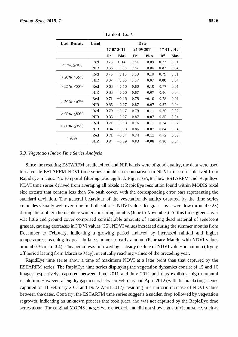
Remote Sens. 2015, 7 6526
Table 4. Cont.
Bush Density Band Date
17-07-2011 24-09-2011 17-01-2012
R2 Bias R2 Bias R2 Bias
> 5%, ≤20% Red 0.73 0.14 0.81 −0.09 0.77 0.01
NIR 0.86 −0.05 0.87 −0.06 0.87 0.04
> 20%, ≤35% Red 0.75 −0.15 0.80 −0.10 0.79 0.01
NIR 0.87 −0.06 0.87 −0.07 0.88 0.04
> 35%, ≤50% Red 0.68 −0.16 0.80 −0.10 0.77 0.01
NIR 0.83 −0.06 0.87 −0.07 0.86 0.04
> 50%, ≤65% Red 0.71 −0.16 0.78 −0.10 0.78 0.01
NIR 0.85 −0.07 0.87 −0.07 0.87 0.04
> 65%, ≤80% Red 0.70 −0.17 0.78 −0.11 0.76 0.02
NIR 0.85 −0.07 0.87 −0.07 0.85 0.04
> 80%, ≤95% Red 0.71 −0.18 0.76 −0.11 0.74 0.02
NIR 0.84 −0.08 0.86 −0.07 0.84 0.04
>95% Red 0.71 −0.24 0.74 −0.11 0.72 0.03
NIR 0.84 −0.09 0.83 −0.08 0.80 0.04
3.3. Vegetation Index Time Series Analysis
Since the resulting ESTARFM predicted red and NIR bands were of good quality, the data were used
to calculate ESTARFM NDVI time series suitable for comparison to NDVI time series derived from
RapidEye images. No temporal filtering was applied. Figure 6A,B show ESTARFM and RapidEye
NDVI time series derived from averaging all pixels at RapidEye resolution found within MODIS pixel
size extents that contain less than 5% bush cover, with the corresponding error bars representing the
standard deviation. The general behaviour of the vegetation dynamics captured by the time series
coincides visually well over time for both subsets. NDVI values for grass cover were low (around 0.23)
during the southern hemisphere winter and spring months (June to November). At this time, green cover
was little and ground cover comprised considerable amounts of standing dead material of senescent
grasses, causing decreases in NDVI values [35]. NDVI values increased during the summer months from
December to February, indicating a growing period induced by increased rainfall and higher
temperatures, reaching its peak in late summer to early autumn (February-March, with NDVI values
around 0.36 up to 0.4). This period was followed by a steady decline of NDVI values in autumn (drying
off period lasting from March to May), eventually reaching values of the preceding year.
RapidEye time series show a time of maximum NDVI at a later point than that captured by the
ESTARFM series. The RapidEye time series displaying the vegetation dynamics consist of 15 and 16
images respectively, captured between June 2011 and July 2012 and thus exhibit a high temporal
resolution. However, a lengthy gap occurs between February and April 2012 (with the bracketing scenes
captured on 11 February 2012 and 19/22 April 2012), resulting in a uniform increase of NDVI values
between the dates. Contrary, the ESTARFM time series suggests a sudden drop followed by vegetation
regrowth, indicating an unknown process that took place and was not captured by the RapidEye time
series alone. The original MODIS images were checked, and did not show signs of disturbance, such as
Remote Sens. 2015, 7 6527
fire or dust. The variability in standard deviations of NDVI values is low in both the RapidEye and
ESTARFM time series during times of low dynamics. Higher standard deviations can be observed during
increment, peak and decrement of the curve, with ESTARFM showing higher deviations than RapidEye
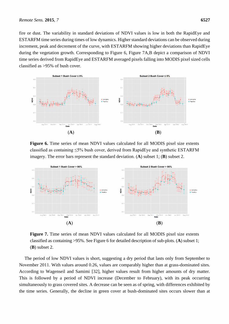
during the vegetation growth. Corresponding to Figure 6, Figure 7A,B depict a comparison of NDVI
time series derived from RapidEye and ESTARFM averaged pixels falling into MODIS pixel sized cells
classified as >95% of bush cover.
(A) (B)
Figure 6. Time series of mean NDVI values calculated for all MODIS pixel size extents
classified as containing ≤5% bush cover, derived from RapidEye and synthetic ESTARFM
imagery. The error bars represent the standard deviation. (A) subset 1; (B) subset 2.
(A) (B)
Figure 7. Time series of mean NDVI values calculated for all MODIS pixel size extents
classified as containing >95%. See Figure 6 for detailed description of sub-plots. (A) subset 1;
(B) subset 2.
The period of low NDVI values is short, suggesting a dry period that lasts only from September to
November 2011. With values around 0.26, values are comparably higher than at grass-dominated sites.
According to Wagenseil and Samimi [32], higher values result from higher amounts of dry matter.
This is followed by a period of NDVI increase (December to February), with its peak occurring
simultaneously to grass covered sites. A decrease can be seen as of spring, with differences exhibited by
the time series. Generally, the decline in green cover at bush-dominated sites occurs slower than at

Remote Sens. 2015, 7 6528
grass-dominated sites. The dip in NDVI values in February 2012 followed by an increase can be
observed in the ESTARFM time series, but not in the RapidEye one (Figure 7A,B).
And again, variability in standard deviations is low during times of no growth, but shows a
discrepancy in phases of vegetation greening. Figure 8A,B shows a comparison of NDVI time series for
the averages of those pixels falling into MODIS pixels containing mixed vegetation communities, with
a percentage of area of bush cover between >50% and ≤65%. Despite the heterogeneity, the overall
compliance of the ESTARFM and RapidEye NDVI time series is good. The curves feature all
characteristics that are mentioned above, in connection with the NDVI values found in homogeneous
areas. Standard deviations exhibit similar dimensions during phases of non-dynamics, and diverge
during times of vegetation growth.
(A) (B)
Figure 8. Time series of mean NDVI values calculated for all MODIS pixel size extents classified
as containing >50% and ≤65% bush cover. See Figure 6 for detailed description of sub-plots.
(A) subset 1; (B) subset 2.
4. Discussion
4.1. Band Differences
We found strong correlations between the observed and predicted RapidEye reflectance values, for
both the red and NIR bands (R2 values range from 0.80 to 0.92 for the red band and from 0.83 to 0.93
for the NIR band). Results suggest that precision is best during phases of low vegetation dynamics, and
deteriorates during phases of strong vegetation growth (December, January). Notably, predictions
generally achieved better results for the NIR band than for the red band. This may be because the
reflected radiation in the NIR is higher for vegetated land surfaces than in the visible wavelength and
hence proportionally less affected by radiation variations. Roy et al. [36], using a different fusion
approach with MODIS and Landsat imagery, observed the same behaviour in their study. They attribute
this to greater influence of atmospheric effects at shorter wavelengths. Rayleigh scattering affects shorter
wavelength more seriously than longer wavelengths [37], and aerosol scattering is frequently more
significant at shorter wavelengths [36]. These findings are also confirmed by Hilker et al. [11], who
found STARFM predictions of shorter wavebands to be less precise than those made for the NIR region
at a coniferous dominated study site in central British Columbia, Canada. Contrary, Walker et al. [10]
observed higher R2 values for the red band than for the NIR band, using STARFM to create synthetic

Remote Sens. 2015, 7 6529
imagery for semi-arid dryland forest and grassland in central Arizona, USA. This suggests that further
testing of the fusion method is needed for a range of sensors/environmental settings to enable the
application value of this approach.
Although we carefully masked out cloud pixels in the RapidEye images, remaining deviating pixel
values might have affected ESTARFM predictions and results of the accuracy assessment, caused by
variations in aerosol loadings and water vapour variations not taken into account by the atmospheric
correction procedure. Furthermore, Schmidt et al. [8] found that erroneous MODIS flag files and data
gaps in the MODIS 8-day image product caused outlying STARFM prediction values. This could be as
well the case in our study.
In almost all cases, the relative mean bias was not equal to 0, with sets of both positive and negative
numbers. We interpret this to be noise likely due to atmospheric and BRDF effects. These results were
also found in the studies by Gao et al. [9]; Hilker et al. [11] and Singh [38].
The bias is a global measurement criterion where the location of the pixel value is not taken into
account. On the contrary, the per-pixel level of error and coefficient of determination are criteria very
sensitive to value changes in the pixel location [31]. A low R2, high per-pixel level of error and a bias of
close to zero would thus mean that pixel values in their location have changed, but the overall distribution
of values has not. This might have occurred in the predicted image dated 09 January 2012, as the relative
mean bias is comparatively low (0.02 and −0.01), but the per-pixel level of error is high (0.07 and 0.07)
and R2 is low (0.84 and 0.83). Visual inspection of the input MODIS image, however, did not reveal any
deviations. The band by band comparison of observed and predicted images for different bush density
classes shows strong relationships, suggesting a good performance of ESTARFM at sub-MODIS scale.
Overall, R2 values are lower than those found in the accuracy assessment conducted for the entire image,
indicating a decline in quality over vegetated areas.
4.2. Evaluation of NDVI Time Series
The comparison of the NDVI time series derived from ESTARFM and RapidEye data shows that the
ESTARFM-predicted temporal sequence reproduces the characteristic phenological dynamics of
different vegetation communities well. The good agreement of RapidEye and ESTARFM-derived curves
for heterogeneous vegetation cover (bush cover between 50% and 65%) indicates good prediction
behaviour at MODIS sub-pixel scale. This assumption is supported by the good correlations found,
although it shows a decline in prediction accuracy with increasing bush density. The comparison
furthermore indicated that the fusion approach provides additional information that would not have been
captured by either MODIS or RapidEye series alone. This is remarkable, because the time series derived
from RapidEye data already contains information from 15 (Subset 1) and 16 (Subset 2) images respectively,
throughout a period of 12 months. However, the ability to predict changes in the fine-resolution images
depends on the capacity of MODIS to capture these changes. If they are too subtle to be captured,
particularly when originating from vegetation structure, stand composition or at sub-pixel ranges, no
algorithm will be able to predict any changes [9,11].
Generally, the NDVI is subject to known and well-documented limitations, such as soil coverage and
soil moisture effects on rangelands and its spatial discontinuity. Additionally, the signal may be hindered
by noise arising from varying atmospheric conditions (such as clouds, ozone, dust and other aerosols)

Remote Sens. 2015, 7 6530
and sun-sensor-surface viewing geometries. A broad variety of strategies, such as data smoothing
techniques, exist to reduce the impacts of these issues [39].
4.3. BRDF Effects
The MODIS MOD09GQ product is generated by selecting pixels matching different criteria from a
number of images collected over a period of 8 days, preferably those taken at a low viewing angle, which
minimizes angular effects. In some images, the reflectance values for adjacent pixels were collected at
different illumination intensities and at different viewing angles and so are subject to high differences.
BRDF effects may also explain the oscillating behaviour of the MODIS time series curve in Figure 5.
Furthermore, the seasonal devolution of the MODIS offset could be caused by these effects. The time
series derived from RapidEye data, whose images are also prone to effects caused by different
illumination and viewing angles (but to a lesser extent due to the swath width of 77 km only), shows less
amplitude, indicating a good performance of the atmospheric correction algorithm. However, the usage
of the NDVI should limit the impact of directional effects, as the signatures in the red and NIR are quite
similar [40]. Walker et al. [10] evaluated the effect of BRDF-adjustment on the accuracy of fused
MODIS-Landsat imagery using STARFM. They found that for NDVI the 8-day composite results were
similar to those of the Nadir BRDF-Adjusted Reflectance (NBAR) 16-day composite data, indicating
that compositing effects only play a minor role for the derivation of indices. The impact of angular effects
on the results is an important topic for a consequent study and could be addressed via radiative transfer
modelling or by using a simple model based on BRDF parameters [40]. To enhance usability and
practical value of medium resolution datasets from MODIS, either BRDF correction should be inherently
included in these products or operational automated tools for BRDF correction should be developed by
the image providers.
4.4. Co-Registration of MODIS and RapidEye Images
We relied on the georeferences provided with the MODIS and RapidEye data. This might have
introduced an error of unknown extent in case good sub-pixel alignment was not achieved between the
datasets. However, the investigation of errors caused by insufficient co-registration was beyond the
scope of this study, but may offer a foundation for further research. We furthermore assume that
ESTARFM’s moving window is able to reduce the effect of co-registration error to some extent.
5. Conclusions and Outlook
The ESTARFM algorithm could successfully be applied for the generation of a high spatio-temporal
vegetation time series by fusing RapidEye and MODIS imagery. The ESTARFM prediction accuracy is
good for the red and NIR bands during phases of little vegetation dynamics, but deteriorates during times
of quick vegetation growth. The NIR band generally yields better prediction results than the red band.
ESTARFM algorithm applied to MODIS and RapidEye imagery shows strong prediction performance
at sub-MODIS scale in heterogeneous vegetated areas, with best results during phases of low vegetation
dynamics. Strategies to reduce noise of NDVI time series may be helpful in future research to reduce
errors caused by variations in atmospheric conditions and BRDF effects.

Remote Sens. 2015, 7 6531
The ESTARFM derived NDVI time series reproduces the characteristic phenological development of
different vegetation types well and inherits more information than either MODIS or RapidEye alone.
The derivation of a complete series of high resolution satellite imagery from both real and synthetic
RapidEye scenes allows to capture temporal variation of vegetation characteristics estimates throughout
the growing season which otherwise cannot be obtained. Due to the combination of large spatial coverage
of the sensor with short term observation intervals and fine spatial resolution, the response of vegetation
to environmental factors and to management can be much better observed and interpreted. So, employing
ESTARFM using the combination RapidEye-MODIS allows for the coverage of spatio-temporal patterns
of vegetation dynamics at small scale that must remain undetected without this technique. Our results
and conclusions might apply to semi-arid rangelands only. The transferability to other landscapes and
vegetation covers can be subject to further studies. An expansion to a longer time series is favourable
and may give further insight to small scale trends over long time periods.
Acknowledgments
This study was carried out as part of the research project “Resilience, Collapse and Reorganisation in
Social-Ecological Systems of African Savannas” (FOR 1501), funded by the German Research
Foundation (DFG). We thank the DLR for the provision of RapidEye data from the RapidEye Science
Archive and for providing access to the CATENA processing system. We are furthermore grateful for
partial funding from the German Federal Ministry of Education and Research (BMBF) in the SPACES
project “Living Landscapes Limpopo”. Thanks to Katharina Brüser for her preceding work.
Author Contributions
Andreas Tewes prepared the data, performed the analysis and wrote the paper. Frank Thonfeld and
Michael Schmidt contributed to the analysis and interpretation of results. Roelof Oomen added
knowledge about the study area. Xiaolin Zhu gave valuable help concerning ESTARFM.
Olena Dubovyk contributed information about BRDF issues and manuscript preparation. Gunter Menz
and Jürgen Schellberg supervised the work and helped structuring the document.
Conflicts of Interest
The authors declare no conflict of interest.
References
1. Fensholt, R.; Sandholt, I.; Rasmussen, M.S. Evaluation of MODIS LAI, fAPAR and the relation
between fAPAR and NDVI in a semi-arid environment using in situ measurements. Remote Sens.
Environ. 2004, 91, 490–507.
2. Pettorelli, N.; Vik, J.O.; Mysterud, A.; Gaillard, J.-M.; Tucker, C.J.; Stenseth, N.C. Using the
satellite-derived NDVI to assess ecological responses to environmental change. Trends Ecol. Evol.
2005, 20, 503–510.
3. Reed, B.C.; Brown, J.F.; VanderZee, D.; Loveland, T.R.; Merchant, J.W.; Ohlen, D.O.
Measuring phenological variability from satellite imagery. J. Veg. Sci. 1994, 5, 703–714.

Remote Sens. 2015, 7 6532
4. Busetto, L.; Meroni, M.; Colombo, R. Combining medium and coarse spatial resolution satellite
data to improve the estimation of sub-pixel NDVI time series. Remote Sens. Environ. 2008, 112,
118–131.
5. Aplin, P. Remote sensing: Ecology Prog. Phys. Geogr. 2005, 29, 104–113.
6. Brüser, K.; Feilhauer, H.; Linstädter, A.; Schellberg, J.; Oomen, R. J.; Ruppert, J. C.; Ewert, F.
Discrimination and characterization of management systems in semi-arid rangelands of South
Africa using RapidEye time series. Int. J. Remote Sens. 2014, 35, 1653–1673.
7. Watts, J. D.; Powell, S. L.; Lawrence, R. L.; Hilker, T. Improved classification of conservation
tillage adoption using high temporal and synthetic satellite imagery. Remote Sens. Environ. 2011,
115, 66 – 75.
8. Schmidt, M.; Udelhoven, T.; Gill, T.; Röder, A. Long term data fusion for a dense time series
analysis with MODIS and Landsat imagery in an Australian Savanna. J. Appl. Remote Sens. 2012,
6, doi:10.1117/1.JRS.6.063512.
9. Gao, F.; Masek, J.; Schwaller, M.; Hall, F. On the blending of the Landsat and MODIS surface
reflectance: Predicting daily Landsat surface reflectance. IEEE Trans. Geosci. Remote Sens. 2006,
44, 2207–2218.
10. Walker, J.J.; de Beurs, K.M.; Wynne, R.H.; Gao, F. Evaluation of Landsat and MODIS data fusion
products for analysis of dryland forest phenology. Remote Sens. Environ. 2012, 117, 381–393
11. Hilker, T.; Wulder, M.A.; Coops, N.C.; Seitz, N.; White, J.C.; Gao, F.; Masek, J.G.; Stenhouse, G.
Generation of dense time series synthetic Landsat data through data blending with MODIS using a
spatial and temporal adaptive reflectance fusion model. Remote Sens. Environ. 2009, 113, 1988–1999.
12. Zhu, X.; Chen, J.; Gao, F.; Chen, X.; Masek, J.G. An enhanced spatial and temporal adaptive
reflectance fusion model for complex heterogeneous regions. Remote Sens. Environ. 2010, 114,
2610–2623.
13. Kim, J.; Hogue, T.S. Evaluation and sensitivity testing of a coupled Landsat-MODIS downscaling
method for land surface temperature and vegetation indices in semi-arid regions. J. Appl. Remote
Sens. 2012, 6, doi:10.1117/1.JRS.6.063569.
14. Pohl, C.; van Genderen, J.L. Review article Multisensor image fusion in remote sensing: Concepts,
methods and applications. Int. J. Remote Sens. 1998, 19, 823–854.
15. Hansen, M.C.; Roy, D.P.; Lindquist, E.; Adusei, B.; Justice, C.O.; Altstatt, A. A method for
integrating MODIS and Landsat data for systematic monitoring of forest cover and change in the
Congo Basin. Remote Sens. Environ. 2008, 112, 2495–2513.
16. Walker, J.J.; de Beurs, K.M.; Wynne, R.H. Dryland vegetation phenology across an elevation
gradient in Arizona, USA, investigated with fused MODIS and Landsat data. Remote Sens. Environ.
2014, 144, 85–97.
17. Emelyanova, I.V.; McVicar, T.R.; Niel, T.G.V.; Li, L.T.; van Dijk, A.I.J.M. Assessing the accuracy
of blending Landsat—MODIS surface reflectances in two landscapes with contrasting spatial and
temporal dynamics: A framework for algorithm selection. Remote Sens. Environ. 2013, 133, 193–209.
18. Zhang, F.; Zhu, X.; Liu, D. Blending MODIS and Landsat images for urban flood mapping.
Int. J. Remote Sens. 2014, 35, 3237–3253.

Remote Sens. 2015, 7 6533
19. Schmidt, M.; Lucas, R.; Bunting, P.; Verbesselt, J.; Armston, J. Multi-resolution time series imagery
for forest disturbance and regrowth monitoring in Queensland, Australia. Remote Sens. Environ.
2015, 158, 156–168.
20. Settle, J.J.; Drake, N.A. Linear mixing and the estimation of ground cover proportions.
Int. J. Remote Sens. 1993, 14, 1159–1177.
21. Mucina, L.; Rutherford, M.C. The Vegetation of South Africa, Lesotho and Swaziland;
South African National Biodiversity Institute: Pretoria, South Africa, 2006.
22. Van Rooyen, N.; Bezuidenhout, H.; De Kock, E. Flowering plants of the Kalahari dunes; Ekotrust:
Pretoria, South Africa, 2001.
23. Palmer, A.R.; Ainslie, A.M. Grasslands of South Africa. In Grasslands of the World; Suttie, J.M.,
Reynolds, S.G., Batello, C., Eds.; Food and Agriculture Organization of the United Nations: Rome,
Italy, 2005; pp. 77–120.
24. Trodd, N.M.; Dougill, A.J. Monitoring vegetation dynamics in semi-arid African rangelands:
Use and limitations of Earth observation data to characterize vegetation structure. Appl. Geogr.
1998, 18, 315–330.
25. Tyc, G.; Tulip, J.; Schulten, D.; Krischke, M.; Oxfort, M. The RapidEye mission design.
Acta Astronaut. 2005, 56, 213–219.
26. RapidEye AG Satellite Imagery Product Specifications, Version 4.1. Available online:
http://www.gisat.cz/images/upload/c1626_rapideye-image-product-specs-april-07.pdf (accessed on
2 September 2014)
27. Krauß, T.; d’ Angelo, P.; Schneider, M.; Gstaiger, V. The fully automatic optical processing system
CATENA at DLR. Int. Arch. Photogramm. Remote Sens. Spat. Inf. Sci. 2013, XL-1/W1, 177–183.
28. Richter, R.; Schläpfer, D. Atmospheric/Topographic Correction for Satellite Imagery: ATCOR-2/3
User Guide, Version 8.2.3; ReSe Applications Schlapfer: Langeggweg, Switzerland, 2012.
29. MODIS MOD09Q1 Product Description. Available online: https://lpdaac.usgs.gov/
products/modis_products_table/mod09q1 (accessed on 21 May 2015).
30. Wald, L.; Ranchin, T.; Mangolini, M. Fusion of satellite images of different spatial resolutions:
Assessing the quality of resulting images. Photogramm. Eng. Remote Sens. 1997, 63, 691–699.
31. Thomas, C.; Wald, L. Comparing distances for quality assessment of fused images.
In New Developments and Challenges in Remote Sensing; Bochenek, E., Ed.; Millpress: Varsovie,
Poland, 2007; pp. 101–111.
32. Wagenseil, M.; Samimi, C. Woody vegetation cover in Namibian savannahs: A modelling approach
based on remote sensing. Erdkunde 2007, 61, 325–334.
33. Scholes, R.J.; Walker, B.H. An African Savanna: Synthesis of the Nylsvley Study; Cambridge
University Press: Cambridge, UK, 1993.
34. Schmidt, H.; Karnieli, A. Remote sensing of the seasonal variability of vegetation in a semi-arid
environment. J. Arid Environ. 2000, 45, 43–59.
35. Weiss, J.L.; Gutzler, D.S.; Coonrod, J.E.A.; Dahm, C.N. Long-term vegetation monitoring with NDVI
in a diverse semi-arid setting, central New Mexico, USA. J. Arid Environ. 2004, 58, 249–272.
36. Mather, P.M. Computer Processing of Remotely-Sensed Images, 3rd ed.; John Wiley & Sons, Ltd:
Chichester, UK, 2004.

Remote Sens. 2015, 7 6534
37. Roy, D.P.; Ju, J.; Lewis, P.; Schaaf, C.; Gao, F.; Hansen, M.; Lindquist, E. Multi-temporal
MODIS-Landsat data fusion for relative radiometric normalization, gap filling, and prediction of
Landsat data. Remote Sens. Environ. 2008, 112, 3112–3130.
38. Singh, D. Evaluation of long-term NDVI time series derived from Landsat data through blending
with MODIS data. Atmósfera 2012, 25, 43–63.
39. Hird, J.N.; McDermid, G.J. Noise reduction of NDVI time series: An empirical comparison of
selected techniques. Remote Sens. Environ. 2009, 113, 248–258.
40. Bréon, F.-M.; Vermote, E. Correction of MODIS surface reflectance time series for BRDF effects.
Remote Sens. Environ. 2012, 125, 1–9.
© 2015 by the authors; licensee MDPI, Basel, Switzerland. This article is an open access article
distributed under the terms and conditions of the Creative Commons Attribution license
(http://creativecommons.org/licenses/by/4.0/).