Using Mathcad to Evaluate View Factors and Orbital Heats for

General Surfaces of Revolution

by

J. T. Pinckney

Jacobs Engineering ESCG

2224 Bay Area Boulevard

Houston, Texas 77058 Phone (281) 461-5434

john.pinckney@escg.jacobs.com

Abstract

The general integral for calculating view factors is presented along with its evaluation using

Mathcad. The method is applicable to any surface that has an analytical definition for the surface

normal vector and is not self viewing. Techniques are discussed on adapting the integral for

general use. Examples are presented and limitations discussed. The method is extended to the

calculation of spacecraft orbital heats.

1.0 Introduction

Many closed form solutions exist for the calculation of the view factor [1]. These solutions are

limited to cases where the surface area integration can be evaluated and the surfaces have

geometric relationships that are conducive for change of variables techniques. Specialized

computer programs have been developed to calculate view factors either by numerical evaluation

of the integral or by Monte Carlo ray casting techniques. These programs remain specialized,

requiring specific training, are not necessarily intuitive in approach and are generally costly.

Furthermore these programs have a limited variety of surface types they can handle.

A view factor integral is presented for use in Mathcad [2], a generally available engineering

mathematics program. The integral is easy to read, understand and alter, requiring only general

Mathcad skills. The integral can be applied to general surfaces of revolution. Shadowing presents

limitations to the method. Techniques are presented to overcome this limitation in some

situations.

The method is extended for use in evaluating spacecraft orbital heats. Any conical section orbit

can be analyzed with a spacecraft surface at any orientation in either the spacecraft coordinate

system or the celestial coordinate system. All orbit parameters are readily modified. Solar

heating calculations can account for orbit intersections with the umbral cone. Planetary heat

calculations can accommodate transitions through the terminator as well as the assumption of

solar inclination anlge dependence of the heats. This integral formulation can be used for quick

orbit evaluations and spot checking Monte Carlo results. The method is limited to direct heating

calculations.

2.0 The View Factor Integral

The general integral to calculate view factor for surface i to surface j is given by Eq.(1) [1].

Eq.(1)

Where ni, nj are surface unit normal vectors, r is a vector from a point on surface i to a point on

surface j. The integration is taken over areas of the surfaces that are viewable from the other

surface. The negative sign accounts for the reversal of r when viewing dAj from dAi.

The task of evaluating Eq.(1) becomes one of formulating the differential areas, limits of

integration and the spatial dependence of the vectors. This formulation is possible, not only for

the limited set of surfaces types available in commercial Monte Carlo codes, but to the much

larger set of all revolved surfaces and in fact any surface that an analytical expression for surface

normal can be formulated. The formulation is most easily accomplished for surfaces that do not

have view factors to themselves and situations where shading is not involved. But in some cases,

as shown in examples below, can be handled with proper limits of integration or with a binary

conditional statements within the integral.

The integral formulation is easily adapted to situations where one surface moves or is rotated

with respect to the other. Spatial variations are accomplished through use of rotational matrices,

variable limits on integration, and linear transformations. Some of these techniques are

demonstrated in the examples.

2.0 View Factor Examples

In the examples below Monte Carlo results are occasionally included for comparison. These

were calculated with Thermal Desktop [4]. Unless otherwise stated 5000 rays per surface was

used in the calculations.

2.1 Parallel Plates of Equal Areas with Aligned Centers with Varying Separation Distance

This is most easily accomplished by defining r as a function of separation distance d.

Fij1

Ai

AjAi

ni r nj r

r r( )2

d d

Eq.(3)

Figure 1 Parallel plates with varying separation distance d.

r xi xj zi zj

xj xi

d

zj zi

Figure 2 View Factor of Parallel Square Plates with Varying Distance Between Plates.

Plate edges are 5 units long.

2.2 Parallel Plates of Equal Areas with Initially Aligned Centers One Plate Moving Along

an Edge

In this example a variable was used in the limits of integration.

Figure 3 Parallel plates with one plate moving in direction parallel to edge.

Figure 4 View Factor of Parallel Square Plates with One Plate Moving Along an Edge.

Edge length equals 5. Calculated using a variable in integration limits.

2.3 Parallel Plates of Equal Areas with Aligned Centers With One Plate Rotated About

Axis Through Centers.

Figure 5 Parallel Plates of Equal Areas With One Plate Rotated About Central Axis.

Figure 6 View Factor of Parallel Square Plates with One Plate Rotated About Center Axis.

This was accomplished by using a rotation matrix to alter the i surface variables in the r

vector.

2.4 Parallel Plates of Equal Areas with Initially Aligned Centers One Plate Rotated About

Axis Perpendicular to Plates and Located at a Corner

Figure 7 Aligned Parallel Plates With One Plate Rotated About Axis Through Opposing

Corners.

Figure 8 View Factor of Parallel Square Plates with One Plate Rotated Around Corner.

2.5 Plates of Equal Areas with Initially Aligned Centers With One Plate Rotated About an

Edge

Figure 9 Parallel Plates with One Plate Rotated About An Edge.

Figure 10 View Factor Initially Parallel Square Plates with One Plate Rotated About an

Edge. This was achieved by using rotation matrix on ith surface coordinates in r vector

definition.

2.6 Parallel Cylinder and Plate of Equal Heights with Plate Moving Parallel (along an) to

Edge Perpendicular to Cylinder Axis

Figure 11. Plate and Parallel Cylinder.

Figure 12 View Factor of Cylinder and Plate with Plate Moving in Line with Edge.

The normal vector, nc, of the cylinder was defined in cylindrical coordinates. It was not

necessary to formulate the integral with complex limits of integration. The positions on the

cylinder not visible to the plate did not contribute to the integral because a conditional statement

within the integral Eq.(4).

Eq.(4)

The if conditional stipulates that if the dot product, nc*r, is greater than 0 then 1 is returned, else

0.

2.7 Partially Closed Cylinder to Itself

Figure 13 View Factor of Partial Cylinder to Itself as Opening Angle Varies.

Figure 14 View Factor of Partial Cylinder to Itself.

if nc i r i yj zi zj 0 1 0

2.8 Identical Planar Cylinders Located on a Hub

Figure 15 Cylinders Located on Hub at Varying Angles.

Figure 16 View Factor of Identical Cylinders Located on a Hub.

3.0 Keplerian Orbital Mechanics and Calculation of Orbital Heats

One of the surfaces in the view factor integral can be a planet surface and the other surface a

spacecraft surface in orbit about the planet. The integration takes place over the viewable area of

the planet, the view cone. The basic formulation is stated in Eq.(5). Planet radius is assumed

equal to 1.

Eq.(5)

where Ai is the surface area, ni is the surface normal vector, r is a the vector from the planet

center to point on its surface, ra is the vector from the planet surface to the spacecraft. R is the

radius of the intermediate view cone and Rv is the view cone radius. t is azimuthal angle of

integration.

qir1

Ai

0

Rv

R

0

2ni ra r ra

ra ra2

R

1 R2

d d

Figure 17 View Cone and Variables of Integration Used to Calculate Planetary Heats.

The integral can be amended to account for surface areas that do not have full view of the view

cone and for view cones that intersect the terminator and for the inclination angle dependence of

planetary heats. Integration over the spacecraft surface is also included. Eq.(6) shows the

resulting integral.

Eq.(6)

qir( )S

Ai

0

Rv( )

R

0

2

0

htr

zi

0

2

i

ni i ra R( ) r R( ) ra R( ) 1( ) z r R( ) if r R( )3

0 1 0 if ni i ra R( ) 0 1 0

ra R( ) ra R( )2

dAiR

1 R2

d d d d

3.1 General Form of Orbits in Cylindrical Coordinates

The general form of the orbit equation is given by

Eq.(7)

Where e is eccentricity and d is distance to directrix. For elliptical orbits 0 < e <1.

3.2 Elliptical Orbits

The example elliptical orbit discussed in the sections below has e = 0.4 and d = 5. The planet

radius is 1. Orbit period is 1. Rotation matrices are employed to orient the orbit in the celestial

coordinate system. These transformations can be described in traditional orbital mechanic terms

of β angle and line of nodes.

Figure 18 Polar Plot of an Example Orbit. The periapsis is at the sub-solar point. A planet

of radius 1 is located at the focus.

3.2.1 Equal Areas in Equal Time Calculations

By the conservation of angular momentum an object in orbit sweeps outs equal area per unit of

time. Dividing the orbit into equal swept areas allows the mapping orbit position dependent

functions to be defined in terms of time. The root function in Mathcad is applied to the function

of Eq.(8) to find orbit points of equal areas.

rr( )d e

1 e cos ( )

Eq.(8)

Figure 19 Example Elliptical Orbit with Equal Sweep Areas Indicated.

f 2

1

2

1

2

d e

1 e cos ( )

2

d A

Figure 20 Orbit Time vs Orbit Angle. Angle is measured from periapsis.

3.3 Solar Heating Examples

3.3.1 Orbit in Elliptic and Periapsis at Sub-Solar Point

The Mathcad root function is used to find the entry and exit points of the umbral cone.

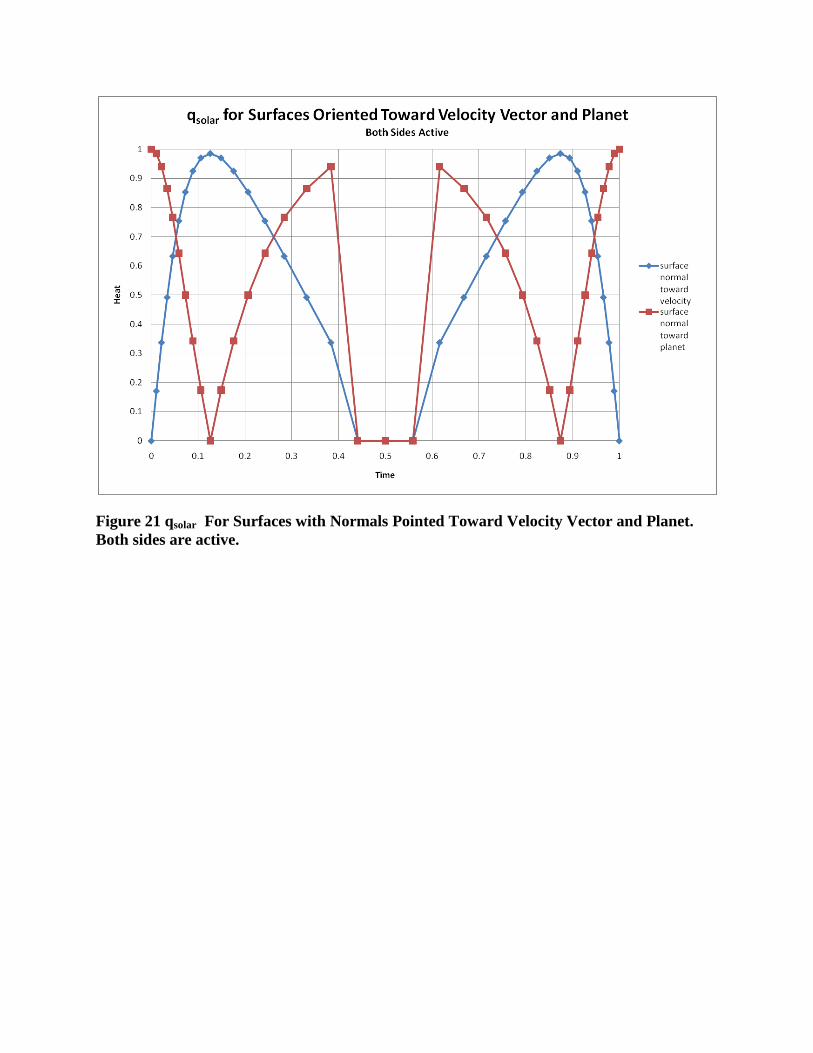
Figure 21 qsolar For Surfaces with Normals Pointed Toward Velocity Vector and Planet.

Both sides are active.

5.2.1.1 Orbit in Elliptic and Periapsis at 60° from Sub-Solar Point

Figure 22 Orbit in Elliptic With Periapsis Rotated 60o from Sub-Solar Point.

Figure 23 Same as Figure 20 but with orbit rotated 60o from solar vector.

Rotation of the orbit is accomplished by matrix multiplication on the solar vector.

3.3.2 Planetary Heating Examples

Under adiabatic regolith and diffuse reflection assumptions the infra-red and albedo heat fluxes

are given by

Eq.(9)

Eq.(10)

where γ is the angle off the sub-solar point. In the planetary heat integral the cos(γ) term is

accounted for in the dot product S*r between the solar vector and the planet surface vector.

Figure 24 Spacecraft Surface and Orbit. The cosine dependence of infra-red or albedo

planetary heat is indicated by the color contours. Also shown is the view cone of the planet

at one orbit position. The Mathcad integral incorporates a conditional statement to

account for that portion of the view cone in the planet shadow.

Planetary heats are calculated by integrating over the view cone at each orbit position. Heats are

calculated by adding heats from two integrals that separately calculate the heat contributions

from the illuminated and shaded sides of the planet. Binary conditional statements are used in the

integrals to account for portions of the spacecraft surface that are in, or not, in view of the planet

and portions of the view cones that are illuminated or shaded.

5.2.3.1 Spacecraft Surface Fixed in Celestial Coordinate System

IRplanet S 1( ) cos ( )

Albedoplanet S cos ( )

A right-handed celestial coordinate system is defined for reference, with the z axis pointed at the

vernal equinox and the y axis in the direction of the elliptic normal. The example orbit is

considered with the following rotations:

Rz(40°)Rx(20°)Ry(30°) Eq.(11)

this results in a β = 33.3° and a solar-periaspsis angle of 35.5°. The analysis was run for a plate

surface fixed in the celestial coordinate system with a normal vector:

Eq.(12)

The results are shown in Figure 26.

Figure 25 View of Orbit and Spacecraft Surface From Orbit Normal. The orbit does not

intercept the umbral cone.

ni

0.224

0.375

0.9

Figure 26 Planetary Infra-red for Illuminated and Shadowed Planet Regions for Fixed in

Celestial Coordinate System. The transition between the illuminated and shadowed planet

regions is captured. The infra-red constant is one tenth of the solar constant in this

example.

4.0 Conclusions

Mathcad has proven to be a useful tool for calculating view factors and spacecraft orbital heats.

View factors calculations are straight forward for any surface that has an analytical formulation

and is not self viewable. This includes most revolved surfaces, including revolutions of all conic

sections. In some cases shadowing can be accounted for by a simple conditional statement placed

in the integral. The view factor integral is easily adaptable to calculate view factors as functions

of rotations and translations of surfaces with respect to one another.

The view factor integral combined with orbit functions can be used to calculate solar and

planetary orbital heats. Surfaces can be oriented in the spacecraft or celestial coordinate systems,

orientation can be easily adapted to be time dependent. All common spacecraft surface types can

be accounted for. Shadowing by other surfaces would require special techniques. All conic

section orbits are readily handled.

The orbital heat calculations capture transitions through the planet terminator and the solar

inclination angle dependence of albedo and infra-red heats. Rotation of matrices can be used to

vary orbit inclination. E.g the solar vector can be rotated to analyze the variations in orbital heat

averages throughout the year or orbital maximum heats can be calculated as a function of β

angle. The method is useful for rapid parametric analysis of orbits and as screening tool for

detailed Monte Carlo models [5].

Using the methods presented here gives the student an intuitive feel for view factors and is an

excellent tool to acquaint oneself with orbital mechanics and the phenomenon of orbital heating.

5.0 Nomenclature

T orbit period

θ orbit angle

a semi-major axis

b semi-minor axis

d distance, distance to directrix

e eccentricity

t time

r sight vector between surfaces, planet center vector

ra vector from planet surface to spacecraft

R radius of differential view cone

Rv radius of view cone

ni,j surface normal vectors

rr orbit distance

Rx, Ry, Rz rotation matrices

t azimuthal angle of view cone

qsolar solar heat

qir infra-red heat

θi,j surface azimuthal angle

Ai,j surface area

S solar vector

6.0 References

[1] Siegal, Robert, Howell, John R., “Thermal Radiation Heat Transfer”; Taylor & Francis,

3rd

edition, 1992

[2] MathCad 14.0 MO3O, Parametric Technology Corporation, 140 Kendrick Street,

Needham, MA 02494 USA

[3] Incropera, F.P, DeWitt, D.P., “Fundamentals of Heat Transfer and Mass Transfer”;

John Wiley & Son, 4th edition, 1996

[4] Thermal Desktop 5.2 Patch 3

[5] Rickman, S.L., “A Simplified Closed-Form Method for Screening Spacecraft Orbital

Heating Variations”; Proceedings Thermal Analysis and Fluid Workshop 2002