Using Engel Curves to Estimate the Bias in the Australian CPI

Using Engel Curves to Estimate the Bias in theAustralian CPI∗

Garry F. BarrettSchool of Economics

University of New South WalesSydney, NSW, [email protected]

andMatthew Brzozowski

Department of EconomicsYork University

Toronto, Ontario, M3J [email protected]

This draft: October 2008.

AbstractThe Australian CPI is a Laspeyres price index which is subject to a number of well-known biases. This paper evaluates the performance of the Australian CPI as a truecost of living index by comparing CPI-deflated food Engel curves estimated with theAustralian Bureau of Statistics Household Expenditure Surveys. Our findings indicatethe Australia CPI overstated changes in the general cost of living by 34% between 1975/76-2003/04. The CPI was especially inaccurate for single adults and lone mother families.In contrast, the CPI was relatively accurate in measuring changes in the cost of livingfor two-adult and working families.

JEL classifications: C1; C43; D12Keywords: CPI bias; Cost of Living; Engel curves; Prices

∗Comments from Martin Browning, participants at the Econometric Society of Australasia Meetingsin Wellington 2008 and a seminar at Macquarie University are gratefully acknowledged. The usualdisclaimer applies.

1

1 INTRODUCTION

Assessing the performance of an economy over time relies on the accurate measurement of

price changes. The measurement of changes in real GDP over time, productivity growth,

changes in real wages and household income all depend on a measure of the change in

nominal prices. The most widely used price deflator is the consumer price index (CPI).

The Australian CPI is compiled by the Australian Bureau of Statistics (ABS) and is a

Laspeyres-type index which has fixed quantity weights for different commodity groups

based on expenditure patterns observed in an earlier period. Laspeyres price indices are

subject to a number of well-known biases (including substitution, outlet, new good and

quality bias) which were highlighted in the Boskin Report (1996) for the United States

(US).

This paper evaluates the performance of the Australian CPI as a true cost of living

index. The analysis is based on ‘Engel’s Law’ which states that, other things equal, the

share of a household’s budget devoted to food declines as total expenditure increases.

Engel’s law has formed the basis of many studies of household welfare, where households

are assumed to be equally well off if they devote the same share of their budget to

food. This intuition has provided the basis for studies estimating adult equivalence

scales and poverty thresholds. Engel’s law is an empirical relationship which has been

observed in data from many countries, and within countries over time. As Houthakker

(1987) succinctly summarised, “of all the empirical regularities observed in economic

data, Engel’s Law is probably the best established; indeed it holds not only in the cross-

section data where it was first observed, but has often been confirmed in time-series

analysis as well.”

Hamilton (2001) and Costa (2001) used Engel’s law to estimate the bias in the US

CPI. Their analyses are based on the simple idea that if the CPI is an accurate measure

of the cost of living then CPI-deflated Engel curves (food-share equations expressed as

a function of real expenditure) estimated at different points in time should coincide. Al-

ternatively, drift in the CPI-deflated Engel curves over time will reflect systematic bias

in the measurement of the CPI (after controlling for changes in the relative price of food

and for changes in the composition of the population). This paper adopts and extends

the Hamilton-Costa approach to assessing CPI mismeasurement. We estimate food Engel

2

curves for Australia using the ABS Household Expenditure Surveys (HES) which span

the period 1975/76-2003/04. The Working-Leser specification for Engel curves, with ex-

tensions recommended by Blow (2003), are estimated and the accuracy of the Australian

CPI as a cost of living index (COLI) evaluated.

The main findings are that the Australian CPI overstated average changes in the gen-

eral cost of living by approximately 22% between 1984 - 2003/04 (34% between 1975/76

-2003/04). There is substantial heterogeneity in household-specific inflation rates, and

the CPI was found be especially inaccurate as a measure of changes in the cost of living

for single adults and lone mother families. In contrast, the CPI was found to be a rela-

tively accurate measure of changes in the cost of living experienced by working families

and two-adult families.

2 LITERATURE REVIEW

2.1 The Australian Consumer Price Index

The historical background of the Australian consumer price index (CPI) is detailed in

ABS (2005a). The CPI was introduced in 1960, with the index calculated retrospectively

back to 1948. The original aim of the CPI was to measure changes in retail prices of goods

and services purchased by metropolitan employee households (ABS 2005a: 3). At it’s

inception, the primary purpose of the CPI was to provide a COLI for metropolitan wage-

earnings households. This purpose of the CPI, and prior retail price index series dating

back to the ‘A Series’ first compiled in 1912, reflected it’s role in the wage determination

process in Australia.

The Australian CPI is a Laspeyres index with fixed quantity weights for each com-

modity groups based on past observed expenditure patterns. The CPI is reviewed and

re-weighted approximately every five years. The last substantial review of the CPI co-

incided with the release of the 13th series in September 1998. With this release the

principal objective of the CPI changed from providing a COLI for urban working house-

holds to providing a general measure of price inflation facing the household sector (ABS

2005a). The change in objective reflected the increasingly important role of the CPI as

an input into macroeconomic policy development, especially by the Reserve Bank of Aus-

tralia in setting monetary policy (ABS 2005a: 45). The main consequence of this change

3

for the compilation of the CPI was the exclusion of interest charges and the inclusion

of house purchase prices in the index. The Australian CPI has now been reviewed and

re-weighted fifteen times. The latest CPI series was released in September 2005 and is

based on expenditure patterns recorded in the HES 2003-04 (ABS 2005b: 7).

2.2 Studies of CPI Bias Based on the Engel Curve Method

Hamilton (2001) and Costa (2001) were first to utilize the Engel curve method for as-

sessing CPI bias. They found that for the US economy as a whole, the CPI consistently

overstated changes in the cost of living. Both found that the CPI over-estimated the true

cost of living by approximately 2.5 per cent per year between 1974 and 1981, and slightly

less than 1 per cent per year between 1981 and 19911. These estimates were remarkably

similar to those found by the more elaborate approach taken by the Boskin Commission

which set out to calculate the contribution of each possible source of CPI bias. The

Boskin Commission Report (1996) concluded that in aggregate the CPI overstated the

true inflation rate by approximately 1.1 percent per year on average.

The Hamilton-Costa approach has the potential to uncover CPI mismeasurement

of the cost of living due to substitution bias and outlet bias. The CPI provides a

comparison of the cost of purchasing a fixed basket of commodities in the base period

with the cost of purchasing the same basket in a later period. As the CPI does not

take account consumer’s ability to substitute away from relatively expensive to relatively

cheaper commodities, the CPI will overstate changes in the true cost of living due to

‘substitution bias’. A similar, related form of cost of living mismeasurement is known as

outlet bias. The CPI is constructed from a survey of prices charged at a fixed set of

outlets selected in the base period. Since consumers can substitute away from relatively

expensive outlets to cheaper outlets, the base period sample of outlets will not accurately

reflect where consumers actually make their purchases in later periods. However, as

discussed by Hausman (2003), the Engel curve method will not capture other forms of

bias, such as new product bias or quality change bias,2 which were also considered by

the Boskin Commission. Therefore the Engel curve methodology can be interpreted as

providing a lower bound on the potential bias in the CPI.

1Costa (2001) examined the much longer historical period 1888-1994, and found that the extent ofCPI bias varied considerably across distinct periods.

2The Engel curve method will capture quality bias to the extent that quality changes correspond toimproved product durability (Beatty and Røed Larsen 2005: 484).

4

The first international application of the Hamilton-Costa approach was presented by

Gibson and Scobie (2002). They analyzed New Zealand data and found that despite the

perception of higher quality of New Zealand’s CPI, that index too exceeded changes in

the true cost of living by an amount comparable to that found for the US.

Two Canadian studies, by Beatty and Røed Larsen (2005) and Brzozowski (2006), in-

troduced several extensions to the Hamilton-Costa methodology. Both studies analyzed

the Canadian population as a whole, as well as the experiences of various subgroups of the

population. They found that the Canadian CPI had been a similarly poor measure of the

cost of living for the general population as well as for the demographic groups examined.

Furthermore, Beatty and Røed Larsen (2005) introduced a flexible semi-parametric spec-

ification for the Engel curve, while Brzozowski (2006) used the quadratic in log of real

total expenditure parametric specification suggested (though not fully implemented) by

Costa (2001). The differences between results based on these more flexible specifications

and the original model as developed by Hamilton were negligible.

In contrast, Røed Larsen (2007) found that in Norway the CPI actually understated

changes in the cost of living for some segments of society while it was largely accurate for

others. To our knowledge, this is the only study based on the Hamilton-Costa methodol-

ogy that concludes the CPI under-estimates changes in the cost of living. Røed Larsen

(2007) used both the linear in log income parametric specification of Hamilton, and a

semi-parametric specification similar to that adopted by Beatty and Røed Larsen (2005)

for Canada.

The Hamilton-Costa Engel curve method has also been adopted for analysing the

accuracy of the CPI in the developing world. Gibson, Stillman and Le (2007) analysed

the performance of the Russian economy using both cross-sectional and panel data. The

analysis is primarily based on the conventional parametric linear in log total expenditure

specification for the Engel curve, although they performed a wide range of sensitivity

tests. de Carvalho Filho and Chamon (2007) considered Brazil and Mexico. They

employed the parametric specification of Hamilton and a semi-parametric specification

similar to that used by Beatty and Røed Larsen (2005) and Røed Larsen (2007). Both

studies find that these economies also experienced inflation rates lower than previously

thought and thus a large portion of what was deemed inflation was in fact real economic

growth. In all three countries the results were generally found to be robust to the choice

5

of estimation method.

3 METHODS

Spending on food is the focus of this literature for several reasons. First, food is non-

durable and reported expenditure in even relatively short reporting periods is likely to

correspond closely to consumption. Second, it has been established in many empirical

demand studies that the elasticity of food expenditure with respect to total expenditure

(or income) is significantly less than one (e.g. Theil et al. 1989). It is important that the

elasticity of the commodity is not equal to unity, otherwise it would not be possible to

distinguish between shifts along the Engel curve due to changes in real total expenditures

from shifts of the Engel curve due to mis-measured prices. It is feasible that luxury

goods, such as recreational expenditures, could also be used to measure CPI bias (see

Costa 2000), although, in contrast to food expenditure, such goods are subject to more

difficult definitional issues and the problems of infrequency of purchase. In addition, it

is arguable that food is additively separable from other commodities in consumer utility

functions, which further supports the singular focus on food expenditure.3

The methods used in the analysis build on the Working-Leser specification for the

food budget share defined as a function of the log of total expenditure - the ‘food Engel

curve’. This specification has been widely and successfully used to estimate food share

equations, and is the basis of Deaton and Muellbauer’s (1980) flexible ‘almost ideal’

demand system model. The food budget share ωijt for family i residing in region j at

time t is expressed as

ωijt = φ+ γ ln³pfjt/p

nfjt

´+ β ln (Yijt/pjt) +X

0ijtθ + μijt (1)

where pfjt is the true price of food, pnfjt is a true price of non-food and pjt is the true price

level (which is a weighted average of pfjt and pnfjt ), Yijt is nominal total expenditure and

Xijt is the vector of other covariates. The term ln³pfjt/p

nfjt

´in equation (1) is the log of

relative price of food and the term ln (Yijt/pjt) is the log of real total expenditure.

Following Hamilton (2001) any price level pjt can be decomposed into the true price

3Hamilton (2001: 622) shows that if utility is additively separable in food and non-food groups andthe sub-utility functions are homothetic then it is possible to decompose food and non-food expendituresinto a price and a quantity index. As a consequence, CPI bias in goods such as personal computers willnot affect food’s budget share through unmodeled complementarities or substitutabilities.

6

level and an error term :

ln pjt = ln pj0 + ln(1 +Πjt) + ln(1 +Et) (2)

where pj0 is the true price level at time 0, Πjt is the cumulative percent increase in the

CPI from year 0 to t and Et is the cumulative percent measurement error. It is assumed

that any bias is uniform across regions j. To simplify notation let πjt = ln(1 +Πjt) and

εt = ln(1+Et), substitute these into (2), then substitute the expression from (2) into (1)

to obtain:

ωijt = φ+ γ³πfjt − πnfjt

´+ β (yijt − πjt) +X 0

ijtθ + (3)

γ³εft − εnft

´− βεt + γ

³pfj0 − pnfj0

´− βpj0 + μijt

This model can be estimated by

ωijt = ϕ+ γ³πfjt − πnfjt

´+ β (yijt − πjt) +X 0

ijtθ +TXt=1

δtDt + μijt (4)

where Dt is a time dummy variable equal to one at time t and is zero otherwise. The

coefficients on the time dummies reflect, ceteris paribus, the extent of the cumulative

bias in the CPI from the base period. The terms in equation (3) denoted by subscript 0

are constants and are absorbed into the intercept term in (4).4

It follows that:

δt = γ³εft − εnft

´− βεt (5)

It is further assumed that the bias in the price of food and non-food is equal³εft − εnft = 0

´and hence

εt =−δtβ

. (6)

The accumulated bias in each year (relative to the base year) can then be calculated as:

Biast = 1− expÃ−δtβ

!(7)

Equivalently, the correction factor which multiples the measured CPI in period t to give

the true CPI in period t is

Correctiont = 1−Biast = exp

Ã−δtβ

!(8)

4Note that ϕ = φ+ γ³pfj0 − pnfj0

´− βpj0

7

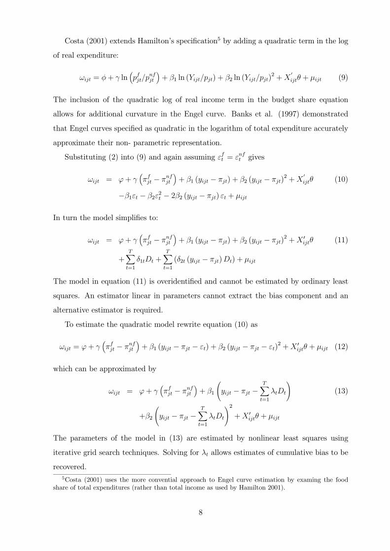
Costa (2001) extends Hamilton’s specification5 by adding a quadratic term in the log

of real expenditure:

ωijt = φ+ γ ln³pfjt/p

nfjt

´+ β1 ln (Yijt/pjt) + β2 ln (Yijt/pjt)

2 +X0ijtθ + μijt (9)

The inclusion of the quadratic log of real income term in the budget share equation

allows for additional curvature in the Engel curve. Banks et al. (1997) demonstrated

that Engel curves specified as quadratic in the logarithm of total expenditure accurately

approximate their nonparametric representation.

Substituting (2) into (9) and again assuming εft = εnft gives


´+ β1 (yijt − πjt) + β2 (yijt − πjt)

2 +X0ijtθ (10)

−β1εt − β2ε2t − 2β2 (yijt − πjt) εt + μijt

In turn the model simplifies to:


´+ β1 (yijt − πjt) + β2 (yijt − πjt)

2 +X 0ijtθ (11)

+TXt=1

δ1tDt +TXt=1

(δ2t (yijt − πjt)Dt) + μijt

The model in equation (11) is overidentified and cannot be estimated by ordinary least

squares. An estimator linear in parameters cannot extract the bias component and an

alternative estimator is required.

To estimate the quadratic model rewrite equation (10) as


´+ β1 (yijt − πjt − εt) + β2 (yijt − πjt − εt)

2 +X 0ijtθ + μijt (12)

which can be approximated by


´+ β1

Ãyijt − πjt −

TXt=1

λtDt

!(13)

+β2

Ãyijt − πjt −

TXt=1

λtDt

!2+X 0

ijtθ + μijt

The parameters of the model in (13) are estimated by nonlinear least squares using

iterative grid search techniques. Solving for λt allows estimates of cumulative bias to be

recovered.

5Costa (2001) uses the more convential approach to Engel curve estimation by examing the foodshare of total expenditures (rather than total income as used by Hamilton 2001).

8

4 DATA AND SAMPLE CONSTRUCTION

Our analysis is based on the Australian Bureau of Statistics Household Expenditure

Survey (HES) unit record files. The HES was conducted in 1975/76, 1984, 1988/89,

1993/94, 1998/99 and 2003/04 (referred to as HES75-HES03). Using the HES data for

the analysis is advantageous given that a key objective of the HES program is to obtain

information on household expenditure patterns in order to revise the commodity weights

underlying the construction of the CPI series.

For the analysis the detailed expenditure information in the HES data (over 600

unique commodity groups are recorded in 2003/04) is aggregated into two broad groups

- food expenditure and total expenditure. Food expenditure includes spending on food

and non-alcoholic beverages, either for consumption at home or outside the home (such

as at cafes or restaurants). The food category explicitly excludes alcoholic beverages and

tobacco. Total household expenditure consists of spending on food, alcohol and tobacco,

current housing costs, fuel and power, household furnishings and equipment, household

services and operations, clothing and footwear, medical care, health and personal care,

transportation, recreation and ‘miscellaneous’ goods and services.6 The food budget

share is simply defined as the ratio of food expenditures to total household expenditures.

Several steps were taken in selecting the analysis sample from the raw HES micro-

data files. First, records for multiple-family households were dropped. Most multiple

family households are comprised of unrelated young adults, and the expenditure informa-

tion which is obtained from interviewing one household member can be very inaccurate.

To minimise reporting errors only single-family households are selected. Approximately

seven percent of observations (2,832 out of a total of 39,498 observations) were excluded

on this criteria7. Observations were also dropped if total expenditure or food expendi-

tures were reported as negative.8 To minimise the influence of extreme observations, the

sample was refined with the top and bottom three percent of observations trimmed from

the distribution of total expenditures and food shares in each survey year.9 In order

6The HES expenditure categories not included in the composite total expenditure bundle are incometax payments, mortgage principal repayments, other capital housing costs, and superannuation and Lifeassurance expenditures (HES expenditure groups 14-17, respectively). These items are excluded becausethey are direct taxes or forms of savings.

7The incidence of multiple-family households within a single cross-section ranged from a high of 15%in HES75 to a low of 4.6 % in HES03.

8These selections resulted in a further 26 and 77 observations, respectively, being dropped.9That is, in each survey the cross-sectional distribution of total expenditure and food shares was

9

to make the geographic coverage of the HES samples as homogeneous as possible, ob-

servations from the Australian Capital Territory (1975/76, 1984, 1993/94, 1998/99 and

2003/04) and the Northern Territory (1993/94, 1998/99 and 2003/04) were dropped from

the sample.10 The sequence of exclusions resulted in a final analysis sample consisting of

30190 observations.

As demonstrated by Blow (2003), it is important to condition on household charac-

teristics when estimating Engel curves. If household characteristics are not adequately

controlled for then differences in estimated food Engel curves over time may reflects

changes in the composition of the underlying population, rather than mismeasurement

of prices. The covariates used in the analysis includes characteristics of the household ref-

erence person (whether female, married, immigrant status, whether employed full-time,

employed part-time or self-employed, whether aged 65 years or older), family character-

istics (indicators for presence of dependent children, presence of students11, whether it

is a lone-parent family, and household size12) and a set of indicator variables for state of

residence.

The HES microdata files were augmented with price information from the ABS CPI

series. The CPI series for three commodity groups - total expenditures, food and non-

food groups - were matched to the HES unit records by survey period (the third quarter

of the survey period for each HES was used13) and state of residence.14 The CPI series

published in ABS (2007: Table 13) were used in the analysis. The reference period

adopted for the CPI bias calculations is 1984, and the reference state is New South

Wales (NSW). The CPI series are rescaled with NSW in 1984 adopted as the base

group.15

trimmed at the 3rd and 97th quantile.10The Northern Territory (NT) was not covered by the 1975/76 or the 1984 surveys. In the 2003/04

survey the Australian Capital Territory (ACT) and NT were not separately identified. As a resultobservations for households recorded as residing in the NT or ACT were excluded. Since the 1988/89survey does not contain an identifier for state or territory of residence, observations from the ACT orNT could not be excluded from this cross-section. A total of 2423 observations were excluded by thisgeographic restriction.11Full-time students aged 15-24 years (except for HES75 and HES84 where it is students aged 15 years

and older).12Household size is top-coded at six in all years.13The analysis was also conducted using the annual average CPI for the four quarters comprising each

HES survey period. The results were invariant to this choice.14Except for the HES88 which included no regional identifiers. The national CPI series was used for

the HES88 sample records.15That is, we divided the CPI series for total expenditure, food and non-food items by the respective

1984 value for New South Wales.

10

Descriptive statistics for the analysis sample are presented in Table 1. The first

column of statistics in Table 1 contains the mean value of the variables for the pooled

sample.16 Additional columns contain the sample means by survey year. For the pooled

sample the average food budget share is 0.214. Reading across the row, the average food

budget share declined over time with each survey. According to ‘Engel’s law,’ the decline

in food shares implies a progressive improvement in the average well-being of Australian

families over the 1975/76-2003/04 period. Average real total household expenditure

(as deflated by the CPI) progressively increased across adjacent surveys except for a

slight decline from 1984-1988/89. Over the full sample period average real household

expenditure is measured to have grown by approximately 21 percent. The relative price

of food (to non-food) increased on average from 1975/76 to 1984, decreased to 1993/94

before increasing from 1993/94 to 2003/04.

Other features of the sample include the increase in the incidence of families with

full-time students, the decline in the incidence of families with children and a decline in

average household size over the observation period. At the same time, there was a rise

in the incidence of single adult and lone parent families, and a corresponding decline in

two-adult or ‘couple’ families. The sample characteristics reflect the demographic trends

in Australian society.

Figure 1 presents partially linear model estimates of the food Engel curve by survey

year. The partially linear model is a semiparametric estimator (see Yatchew 1998, 2003)

with the food budget share specified as a general function of the log of CPI-deflated total

expenditure and a linear function of covariates which include the relative price of food,

reference person and family characteristics. The partially linear model does not restrict

the Engel curves to be a linear or quadratic function of the log of real expenditures. The

figures provide an indication of whether the parametric linear or quadratic specifications

of the Engel curves (in the logarithm of real expenditures) are supported by the data,

and whether there is a shift in the location of the curves over time (revealing systematic

mismeasurement of the CPI). To reiterate, if the official CPI correctly measures changes

in the true cost of living then, given stable preferences and controlling for changes in

relative price of food and demographic effects, the Engel curves estimated from different

16The individual HES contain record weights (which represent the inverse probability of selection intothe survey) which are used in calculating the sample means.

11

time periods will coincide. The amount of drift in the Engel curves over time is then

hypothesised to represent bias in the measurement of the CPI. Figures 1 shows that the

Engel curves based on the sequence of HES84-HES03 are generally parallel, while the

1975 Engel curve has a steeper slope. The estimated Engel curves with the later HES

data are lower and to the left of the earlier surveys. This is interpreted as the official

CPI over-correcting for changes in nominal prices. The distance between the 1984 Engel

curve and that based on other survey years is a measure of cumulative bias in the official

CPI for that year (relative to 1984). The econometric models estimated next quantify

the amount of that bias. The shape of the partially linear model estimates of the Engel

curves suggest that the linear in log of real expenditure specification appears to be a

reasonable approximation to the semiparametric estimates.

The analysis proceeds by estimating CPI bias for the general population. Alternative

specifications for the food Engel curves are considered (linear and quadratic in log of

real total expenditure, with and without the additional covariates). The accuracy of

the CPI as a COLI for a range of specific demographic groups is then examined. The

separate demographic groups considered are non-elderly single persons, adult couples

with no children, adult couples with children, lone mother families, working families and

seniors. In the final section of the analysis, the sensitivity of the bias estimates to a

range of modeling choices, including sample construction, the treatment of conditioning

variables, the use of record weights and model specification, is examined

5 EMPIRICAL RESULTS

5.1 Bias Estimates for the Full Population

Table 2 presents the estimated CPI correction factors17 (and asymptotic standard error

constructed using the delta method) based on the full sample. The first column of

results are for the linear specification of the food Engel curve with controls for the log of

relative prices and the log of real total expenditures only. For this simplified model, the

estimated correction factor for 1975 is 1.19. The interpretation of the correction factor

is that, relative to the 1984 base period, the official CPI for 1975 multiplied by a factor

of 1.19 will produce the true COLI for 1975. Equivalently, the CPI level in 1975 was

under-estimated (and the official inflation rate between 1975 and 1984 over-estimated) by

17Correction factort = 1−Biast = exp(−δt/β).

12

19%. The estimated correction factor for 2003 is 0.58 which in turn indicates cumulative

positive bias in the 2003 official CPI of 42% relative to the 1984 base.

The second set of results are for the linear specification with the full set of covariates.

Conditioning on the full set of individual and family characteristics substantially reduced

the estimated bias in the CPI. The set of covariates are jointly highly statistically sig-

nificant indicating that the bias estimates in model (1) in part reflected shifts over time

in the Engel curves due to changes in the composition of the population. Based on this

superior specification, the 1975 CPI is found to be underestimated by 9% relative to

the 1984 base year. The CPI for 2003 is found to be over-estimated by 18% relative to

1984 (an average annual bias of 1.02% over this period), which in turn implies inflation

between 1984 and 2003 was over-estimated . For the full 1975/76-2003/04 observation

period, the CPI is found to overestimate changes in the true cost of living by 34% (or an

average annual bias of 1.05%).

Several tests where performed for each model. The first test was an F-test of the null

hypothesis that the coefficients on all of the time dummy variables were jointly insignif-

icant (against the alternative that the null is false). A second F-test was performed

for the null that the coefficients on the subset of time dummy variable for 1988-2003

are jointly insignificant. Since an intercept difference may not adequately capture the

difference between the food Engel curve for 1975 and that for later years, this second

hypothesis which did not restrict the coefficient on the 1975 dummy variable, is also con-

sidered. The F-test statistics are reported in the row immediately below the estimated

correction factors. Both null hypotheses were strongly rejected for the linear models at

conventional levels of significance.

The quadratic models specifications were estimated and the implied CPI correction

factors (and asymptotic standard errors) are presented in columns (3) and (4). Again

the model with the full set of covariates produces lower estimates of CPI bias, further

underscoring the importance of controlling for changing population demographics. The

quadratic specification produces a set of correction factors very similar to that found

with the linear specification of the Engel curve. The cumulative bias from in the CPI

from 1984 to 2003 (1975 to 2003) is estimated to be 21% (31%), with an annual average

bias of 0.98% (1.05%). The set of bias estimates are jointly significant, as also found

with the linear model specifications.

13

5.2 Bias Estimates by Demographic Groups

The Engel curve methodology for assessing CPI bias was then used to consider the

accuracy of the CPI for measuring changes in the true cost of living for more narrowly

defined demographic groups. Expenditure patterns vary across family types, and these

models allow the shape of the Engel curves to vary by demographic group.

Figures 2-7 present the partially linear model plots of the Engel curves for non-

elderly single persons, couple families without children, couple families with children,

lone mother families, working families (where an adult member is employed) and seniors

(where the reference person is aged over 65 years), respectively. Table 3 presents the

estimated correction factors based on the quadratic specifications with the full set of

covariates. Several features are evident from the estimates. First, the CPI is found

to be a particularly poor guide to cost of living for single persons and for lone mothers.

The cumulative bias over the period 1984-2003 (1975-2003) for single men and women is

estimated to be 34% (65%) and for lone mothers is 26% (108%). Second, the CPI bias

estimated for seniors mirrors that found for the full sample. Third, the CPI is found to

be a relatively more accurate measure of the cost of living for couple families with and

without children, and particularly for working families. Although the correction factors

for these groups are jointly significant, the point estimates are much smaller in magnitude

for these groups compared to the population as a whole or the other subgroups. For

instance, the estimate of the average annual CPI bias for the cost of living experienced

by working families between 1975 and 2003 is 0.11%, compared to 1.05% for the full

population. Although CPI bias is found to be statistically significant, the magnitude of

the bias estimates suggests that the CPI performed reasonably well as COLI for these

groups. Interestingly, when that objective of the CPI collection changed from being

primarily a COLI in 1998, the point estimates suggest a greater divergence between the

CPI and the cost of living for almost all groups.

5.3 Sensitivity Analysis

The robustness of the empirical finding with respect to a series of model specification

and sample definition choices was examined. The estimated CPI correction factors from

the sensitivity analysis are presented in Table 4. Given that the linear and quadratic

Engel curve models yielded very similar results, the sensitivity analysis was based on

14

the more parsimonious linear Engel curve model.18 First, the model was re-estimated

with the omission of the 1975 data. The Engel curve graphs suggested that a simple

intercept difference may not adequately capture the difference between the Engel curves

between 1975 and the other survey years. This may introduce inconsistency into the

CPI bias estimation for survey years 1988-2003 through the estimated impact of the

covariates. The estimated correction factors for the linear model with the 1975 data

omitted are shown in column (2) of Table 4. The results indicate that the correction

factors are marginally smaller for all the years. However, the point estimates are within

one standard error of, and not statistically different from, the full sample estimates.

The model was then re-estimated with the 1975 data included but the 1988 survey

data excluded. The HES88 data did not include regional identifiers so in this survey year

there is no regional variation in the CPI series. Data from HES88 does not contribute

to the identification of the relative price of food term, and a form of measurement error

may be introduced into the estimation due to aggregation across regions. As shown in

the column (3) of Table 4, the exclusion of the 1988 data resulted in nearly identical

estimates, only the 1998 estimate is marginally, and not significantly smaller from the

estimate based on the full set of HES surveys.

As discussion previously, it is important in Engel curve estimation to include a rich set

of covariates to capture population heterogeneity. Otherwise, changes in the population

(and reflected in the sample) over time will be absorbed into coefficients on the time

dummy variables, and the CPI bias estimates measure true bias and time trends in

the unmeasured characteristics. Although a rich set of covariates were included in the

estimation; richer information is available in the HES microdata. To check sensitivity

of the estimation along this dimension, a set of 12 dummy variables for the age of the

household reference person (with age grouped into five-year bands ranging from age 15-19

years, through to age 75-79 years). This set of variables will allow for discrete variation in

the Engel curves over stages of the lifecycle, and control for the ageing of the Australian

population over the sample period. Another variable added to the model was a dummy

variable indicating whether the household owned the home, as opposed to renting. Home

ownership status increased over the 1975-2003 period, and if home owners have different

18Results based on the quadratic specification are almost identical to those based on the linear speci-fication, and are available from the authors on request.

15

food expenditure patterns compared to renters, other things equal, then the measurement

framework may attribute this to CPI bias. The estimated correction factors based on

the extended covariate set are shown in column (4). It is evident that there was a

slight increase in the estimated correction factors for 1975 and 2003, and slightly smaller

correction factors for 1988-1988, relative to the base model. Again, the difference in

estimates are neither large in magnitude nor statistically significant.

Another issue in the estimation of the models is the treatment of record weights for

the microdata. In linear models, if the factors which determine the record weights are

controlled for in the estimation then the results from an unweighted regression will be

unbiased and consistent.19 The models presented so far were obtained using unweighted

estimation. Incorporating the record weights - which are inverse probability weights20 -

into the estimation leads to the results presented in column (5) of Table 4. Again, the

point estimates are very similar to the base model estimates which do not utilize weights,

and hence the conclusions regarding CPI bias measurement are robust to the treatment

of the record weights.

The models presented so far assume that the price elasticity of the food share is

constant across the total expenditure range. This is potentially an overly restrictive

assumption. It is possible that the food price elasticity of demand varies with total

expenditure. In particular the poor may be more responsive to a change in the relative

price of food, and may be more likely to search for cheaper outlets or substitute towards

more cost effective alternatives, than the rich. This would be evident in plots of Engel

curves with a larger difference between curves at lower levels of total expenditure levels

than at higher levels (and where the relative price of food has increased). To allow for

the price elasticity of food to vary across the expenditure range, the basic model (1) can

be expanded with an interaction term between the log of relative food price and log of

real total expenditure:

ωijt = φ+γ ln³P fjt/P

nfjt

´+β1 ln (Yijt/Pjt)+β2

hln³P fjt/P

nfjt

´× ln (Yijt/Pjt)

i+X

0ijtθ+μijt

(14)

While above model cannot be estimated by OLS, it can be estimated using non-linear

19Intuitively, this situation is equivalent to exogenous sample selection.20The record weights in each cross-section were rescaled so that the total weight was the same for each

cross-section.

16

least square. The final column of Table 4 presents the correction factors based estimated

for this expanded specification. Clearly differences between the model that includes the

interaction term (between the relative price of food and total expenditures) and the base

model are minor and insignificant. As such, we find no evidence that poorer household

(those with lower expenditures) are more sensitive in general to relative food price shocks.

To further investigate potential interaction between price and total expenditure elas-

ticities for food, the extended Engel curve model was estimated separately by demo-

graphic group. The estimated correction factors for the model specification in (14) by

demographic group are presented in Table 5. Comparing the estimates for the extended

specification to the base model estimates reveals several patterns. First, the more gen-

eral specification reduces the estimated correction factor for 1975 compared to the base

year 1984, especially for singles and lone mothers, groups for which the CPI was found

to be most inaccurate. Second, the point estimates for the correction factors for survey

years 1988-1998 are very close to those from the base model, while the estimated accu-

mulated CPI bias in 2003 (relative to 1984) is found to be marginally larger with the

extended specification. Third, the estimated correction factors from the more flexible

specification for all the demographic groups considered were not significantly different

from those derived from the base specification. Therefore the inferences drawn from the

base specification for the general population, and for the various demographic subgroups,

are invariant to the specification of the price responsiveness of the Engel curve over the

expenditure distribution.21

Overall, the sensitivity analysis has shown that the estimated correction factors, and

equivalently the estimates of Australian CPI bias, for the full population sample are

insensitive to a wide range of model specification and sample definition issues considered.

6 CONCLUSION

The results of the analysis show that the CPI over-estimated changes in the cost of living

experienced by the Australian population over the 1975/76 - 2003/04 period by approx-

imately 1% per year on average. Sensitivity analysis showed that these estimates are

robust to a range of sample definition, model specification and estimation issues. In par-

21The estimated correction factors for years 1988-2003 were invariant to the exclusion of the 1975survey data from the estimation, for the all the groups examined.

17

ticular, results based on linear and quadratic in log real total expenditure specifications

yield nearly equivalent results. Furthermore specifications that allow for price elasticity

to vary with expenditure are also very similar. Given the heterogeneity in the cost of

living across households, the CPI proved to be an especially inaccurate measure for single

men and women and lone mother families. However, the Australian CPI has been more

successful in tracking changes in the cost of living facing working families, and couple

families, in Australia. While we found significant bias in the CPI as a measure of the cost

of living for these family types, the magnitude of the bias was relatively small compared

to that found for the full Australian population, and found in other countries.

References

[1] Australian Bureau of Statistics (2007) Consumer Price Index Australia, ABS Cata-

logue No. 6401.0

[2] Australian Bureau of Statistics (2005a) Australian Consumer Price Index: Concepts,

Sources and Methods, ABS Catalogue No. 6461.0

[3] Australian Bureau of Statistics (2005b) A Guide to the Consumer Price Index: 15th

Series, ABS Catalogue No. 6440.0

[4] Australian Bureau of Statistics (2004) Household Expenditure Survey, Australia,

2003/2004 Confidentialised Unit Record File, ABS, Canberra.








1984 Confidentialised Unit Record File, ABS, Canberra.

18



[10] Banks, J., Blundell, R. and Lewbel, A. (1997), “Quadratic Engel Curves and Con-

sumer Demand”, Review of Economics and Statistics, vol 79, pp. 769-88.

[11] Beatty, T. and Røed Larsen, E. (2005) “Using Engel curves to estimate bias in the

Canadian CPI as a cost of living index” Canadian Journal of Economics vol.38(2),

pp.482—499.

[12] Blow, L. (2003) “Explaining trends in UK household spending” Institute for Fiscal

Studies Working Paper 03/06

[13] Boskin et al. (1996), “Toward a more accurate measure of the cost of living” Final

Report to the Senate Finance Commission from the Advisory Commission to Study

the Consumer Price Index.

[14] Brzozowski, M. (2006) “Does One Size Fit All? The CPI and Canadian Seniors,”

Canadian Public Policy, vol.32(4), pp.387-411.

[15] Costa, D. (2000), “American Living Standards, 1888—1994: Evidence from Consumer

Expenditures” National Bureau of Economic Research Working Paper no. 7650.

Cambridge, Mass.

[16] Costa, D. (2001), “Estimating real income in the US from 1888 to 1994: correcting

CPI bias using Engel curves,” Journal of Political Economy, vol. 109, pp. 1288-1310.

[17] de Carvalho Filho, I. and Chamon, M. (2007) “The Myth of Post-Reform Income

Stagnation: Evidence from Brazil and Mexico,” International Monetary Fund Work-

ing Paper.

[18] Deaton, A.S. and Muellbauer, J. (1980) “An Almost Ideal Demand System,” Amer-

ican Economic Review, vol. 70(3), pp. 312-26.

[19] Diewert, W. E. (2001) “The Consumer Price Index and index number purpose,”

Journal of Economic and Social Measurement, vol. 27(3-4), pp. 167-248.

[20] Gibson, J., Stillman S. and Le, T. (2007), “CPI bias and real living standards in

Russia during the transition” Journal of Development Economics, forthcoming.

19

[21] Gibson, J., and Scobie, G. (2002), “Are we growing faster than we think? An

estimate of ‘CPI bias’ for New Zealand” mimeograph, University of Waikato.

[22] Hamilton, B. (2001) “Using Engel’s law to estimate CPI bias” American Economic

Review, vol. 91, pp 619-30.

[23] Hausman, J. (2003) “Sources of bias and solutions to bias in the Consumer Price

Index” Journal of Economic Perspectives, vol. 17(1), pp.23—44.

[24] Houthakker, H. (1987) “Engel’s law” in: Eatwell, J., Milgate, M., and Newman, P.

(eds.), The New Palgrave Dictionary of Economics, vol. 2. McMillan, London, pp.

143—144.

[25] Røed Larsen, E. (2007) “Does the CPI Mirror the Cost of Living? Engel’s Law

Suggests Not in Norway” Scandinavian Journal of Economics, vol.109(1), pp.177—

195.

[26] Theil, H., Chung, C.F., and Seale, J. (1989) International Evidence on Consumption

Patterns, Greenwich, JAI Press.

[27] Yatchew, A. (1998) “Nonparametric Regression Techniques in Economics” Journal

of Economic Literature, vol. 36(2), pp 669-721.

[28] Yatchew, A. (2003) Semiparametric Regression for the Applied Econometrician,

Cambridge, Cambridge University Press.

20

Table 1. Summary StatisticsVariable Pooled Sample 1975 1984 1988 1993 1998 2003

Food Share 0.214 0.231 0.226 0.222 0.209 0.207 0.195Ln(expenditure) 5.661 5.579 5.643 5.618 5.649 5.694 5.768Ln(rel price food) -0.013 -0.053 -0.003 -0.031 -0.046 0.014 0.045

DemographicsEmployed 0.592 0.635 0.546 0.561 0.556 0.588 0.673Senior 0.256 0.230 0.264 0.265 0.259 0.249 0.263Student 0.128 0.079 0.104 0.128 0.136 0.151 0.149Female 0.301 0.176 0.190 0.210 0.390 0.385 0.387Married 0.694 0.735 0.730 0.710 0.685 0.670 0.653Immigrant 0.281 0.263 0.279 0.292 0.291 0.277 0.274

Family Type 0.000Single 0.207 0.188 0.171 0.191 0.210 0.229 0.239Couple 0.694 0.763 0.732 0.707 0.680 0.661 0.653Lone Parent 0.063 0.042 0.061 0.062 0.069 0.070 0.070Other 0.035 0.006 0.037 0.040 0.042 0.040 0.038

Children Present 0.412 0.496 0.455 0.438 0.374 0.382 0.363Household Size 2.705 2.887 2.878 2.799 2.626 2.610 2.535

Location*NSW 0.340 0.353 0.350 0.342 0.327 0.331Vic 0.261 0.282 0.272 0.257 0.257 0.248Qld 0.182 0.152 0.163 0.184 0.195 0.204SA 0.089 0.092 0.092 0.089 0.087 0.086WA 0.100 0.092 0.094 0.100 0.106 0.103TAS 0.028 0.029 0.029 0.028 0.028 0.028

Sample Proportion 1.000 0.13213 0.11736 0.19894 0.20265 0.17214 0.17678Observations 30190 3989 3543 6006 6118 5197 5337

Note: * The pooled sample means for location exclude observations from 1988

Table 2. Estimated Correction Factors, Full SampleYear

(1) (2) (3) (4)1975 1.19** 1.09** 1.25** 1.13**

(.06) (.03) (.06) (.03)1984 1.00 1.00 1.00 1.00

- - - -1988 0.95 0.95** 0.97 0.98

(.03) (.03) (.04) (.03)1993 0.80** 0.94** 0.82** 0.96

(.03) (.02) (.03) (.03)1998 0.71** 0.89** 0.69** 0.87**

(.02) (.02) (.02) (.02)2003 0.58** 0.82** 0.54** 0.79**

(.02) (.02) (.02) (.02)

Covariates No Yes No Yes

F-Test I 83.48†† 25.46†† 101.34†† 30.57††

F-Test II 91.75†† 21.09†† 111.84†† 26.80††

Cumulative Bias Estimates (relative to 1984)1975 19% 12% 25% 13%1988 5% 5% 3% 2%1993 20% 9% 18% 4%1998 29% 14% 31% 13%2003 42% 22% 46% 21%

Estimates of Average Annual Bias1975-2003 1.72% 1.05% 1.93% 1.05%1975-1998 1.72% 1.01% 1.95% 1.01%1984-2003 1.81% 1.02% 1.96% 0.98%1984-1998 1.77% 0.91% 1.88% 0.85%

Notes:Standard Errors reported in parentheses.* Denotes individually statistically different from 1.0 at the 10% significance level and ** denotes individually statistically different from 1.0 at the 5% significance level. †† Denotes joint significance at the 1% level.F-Test I is the test statistic for the null that the coefficients on D1975-D2003 are jointly equal.F-Test II is the test statistic for the null that the coefficients on D1984-D2003 are jointly equal.

Linear Model Quadratic Model

Table 3. Estimated Correction Factors by Demographic GroupYear Group

Singles Couples no kids Couples with kids Lone Mothers Working Families Seniors1975 1.31** 0.96 1.06 1.82** 0.97 1.11

(.12) (.06) (.05) (.34) (.04) (7.00)1984 1.00 1.00 1.00 1.00 1.00 1.00

- - - - - -1988 1.02 0.88** 0.95 1.11 0.93** 0.99

(.08) (.05) (.04) (.15) (.03) (.06)1993 0.95 0.88** 1 0.97 0.96 0.97

(.07) (.05) (.04) (.13) (.03) (.05)1998 0.77** 0.94** 0.95* 0.89 0.99 0.84**

(.05) (.04) (.03) (.09) (.03) (.04)2003 0.66** 0.95 0.88** 0.74** 0.94* 0.78**

(.06) (.05) (.04) (.10) (.03) (.04)

F-Test I 9.39†† 3.29† 4.31† 3.47† 3.14†† 6.88††

F-Test II 8.47†† 2.25 9.39†† 2.42† 3.88†† 7.00††

Cumulative Bias Estimates (relative to 1984)1975 31% -4% -6% 82% -3% 11%1988 -2% 12% 5% -11% 7% 1%1993 5% 12% 0% 3% 4% 6%1998 23% 6% 5% 11% 1% 16%2003 34% 5% 12% 26% 6% 22%

Estimates of Average Annual Bias1975-2003 1.80% 0.04% 0.21% 2.65% 0.11% 1.02%1975-1998 1.90% 0.09% -0.04% 2.90% -0.09% 1.04%1984-2003 1.51% 0.25% 0.58% 1.19% 0.30% 1.02%1984-1998 1.44% 0.40% 0.34% 0.72% 0.07% 1.03%

Notes:Based on Quadratic specification with covariatesStandard Errors reported in parentheses.* Denotes individually statistically different from 1.0 at the 10% significance level and ** denotes individually statistically different from 1.0 at the 5% significance level. †† Denotes joint significance at the 1% level and † denotes joint significance at the 5% level.F-Test I is the test statistic for the null that the coefficients on D1975-D2003 are jointly equal.F-Test II is the test statistic for the null that the coefficients on D1984-D2003 are jointly equal.

Table 4. Estimated Correction Factors, Linear Engel Curves

Specification Base Exclude 1975 Exclude 1988 Extra Covariatesa Weighted Interaction(1) (2) (3) (4) (5) (6)

1975 1.09** 1.09** 1.11** 1.09** 1.10**(.03) (.03) (.03) (.04) (.03)

1984 1.00 1.00 1.00 1.00 1.00 1.00- - - - - -

1988 0.95** 0.94** 0.95** 0.96** 0.98(.03) (.03) (.03) (.03) (.02)

1993 0.94** 0.93** 0.94** 0.94** 0.93** 0.96*(.02) (.03) (.03) (.02) (.03) (.02)

1998 0.89** 0.88** 0.88** 0.88** 0.89** 0.87**(.02) (.02) (.02) (.02) (.02) (.02)

2003 0.82** 0.81** 0.82** 0.80** 0.81** 0.76**(.02) (.02) (.02) (.02) (.03) (.02)

Notes:Based on Linear specification with covariatesStandard Errors reported in parentheses.* Denotes individually statistically different from 1.0 at the 10% significance level and ** denotes individually statistically different from 1.0 at the 5% significance level. a. The additional covariates are a set of 12 indicator variables for the age of the household reference person and a dummy variable for home ownership status.

Tabl

e 5.

Est

imat

ed C

orre

ctio

n Fa

ctor

s by

Dem

ogra

phic

Gro

up, E

xten

ded

Spec

ifica

tion

Yea

rG

roup

Bas

eIn

tera

ctio

nB

ase

Inte

ract

ion

Bas

eIn

tera

ctio

nB

ase

Inte

ract

ion

Bas

eIn

tera

ctio

nB

ase

Inte

ract

ion

1975

1.36

**1.

19*

0.97

1.01

1.10

**1.

09**

1.82

**1.

61**

1.01

1.04

1.08

1.10

(.16)

(.10)

(.06)

(.04)

(.05)

(.04)

(.33)

(.24)

(.04)

(.03)

(.07)

(.06)

1984

1.00

1.00

1.00

1.00

1.00

1.00

1.00

1.00

1.00

1.00

1.00

1.00

--

--

--

--

--

--

1988

1.02

0.95

0.88

**0.

940.

970.

991.

101.

120.

961.

000.

960.

99(.1

0)(.0

6)(.0

5)(.0

4)(.0

4)(.0

3)(.1

5)(.1

3)(.0

3)(.0

3)(.0

6)(.0

5)19

930.

930.

83**

0.89

**0.

93*

1.02

1.04

0.96

0.97

0.98

1.02

0.93

0.96

(.09)

(.06)

(.05)

(.04)

(.04)

(.03)

(.13)

(.11)

(.03)

(.03)

(.05)

(.05)

1998

0.79

**0.

75**

0.94

0.93

*0.

94**

0.91

**0.

890.

880.

980.

960.

84**

0.82

**(.0

6)(.0

7)(.0

4)(.0

4)(.0

3)(.0

3)(.0

9)(.0

9)(.0

2)(.0

3)(.0

4)(.0

4)20

030.

70**

0.66

**0.

950.

89**

0.85

**0.

76**

0.75

**0.

71**

0.90

**0.

84**

0.81

**0.

74**

(.08)

(.08)

(.05)

(.05)

(.03)

(.04)

(.09)

(.09)

(.03)

(.03)

(.05)

(.05)

Not

es:

Bas

ed o

n Li

near

spe

cific

atio

n w

ith c

ovar

iate

sS

tand

ard

Err

ors

repo

rted

in p

aren

thes

es.

* D

enot

es in

divi

dual

ly s

tatis

tical

ly d

iffer

ent f

rom

1.0

at t

he 1

0% s

igni

fican

ce le

vel a

nd

** d

enot

es in

divi

dual

ly s

tatis

tical

ly d

iffer

ent f

rom

1.0

at t

he 5

% s

igni

fican

ce le

vel.

Wor

king

Fam

ilies

Sen

iors

Sin

gles

Cou

ples

no

kids

Cou

ples

with

kid

sLo

ne M

othe

rs

.1.1

5.2

.25

.3.3

5B

udge

t Sha

re

100 200 300 400 500 600Real Total Expenditure ($)

1975 1984 1988 1993 1998 2003

Figure 5.1 Engel Curves - Population

.1.1

5.2

.25

.3.3

5B

udge

t Sha

re


1975 1984 1988 1993 1998 2003

Figure 5.2 Engel Curves - Non-elderly Singles

.1.1

5.2

.25

.3.3

5B

udge

t Sha

re


1975 1984 1988 1993 1998 2003

Figure 5.3 Engel Curves - Non-elderly Couples without Kids

.1.1

5.2

.25

.3.3

5B

udge

t Sha

re


1975 1984 1988 1993 1998 2003

Figure 5.4 Engel Curves - Non-elderly Couples with Kids

.1.1

5.2

.25

.3.3

5B

udge

t Sha

re


1975 1984 1988 1993 1998 2003

Figure 5.5 Engel Curves - Lone Mothers

.1.1

5.2

.25

.3.3

5B

udge

t Sha

re


1975 1984 1988 1993 1998 2003

Figure 5.6 Engel Curves - Working Families

.1.1

5.2

.25

.3.3

5B

udge

t Sha

re


1975 1984 1988 1993 1998 2003

Figure 5.7 Engel Curves - Seniors

Using Engel Curves to Estimate the Bias in the Australian CPI

Documents

Transcript of Using Engel Curves to Estimate the Bias in the Australian CPI