Using Electric System Operating Margins and Build Margins ... cost (typically dominated by the cost...
33
This document was commissioned by the UNFCCC secretariat to facilitate the work of the Methodologies Panel of the CDM Executive Board in considering the weighted average of the operating margin (OM) and the build margin (BM) emission factor to calculate the baseline emission factors for projects generating electricity to the grid. Views expressed in this document are those of the author and do not necessarily represent the views of the United Nations, the UNFCCC secretariat, the Methodologies Panel or the CDM Executive Board. Using Electric System Operating Margins and Build Margins in Quantification of Carbon Emission Reductions Attributable to Grid Connected CDM Projects Prepared by: Bruce Biewald Synapse Energy Economics 22 Pearl Street, Cambridge, MA 02139 www.synapse-energy.com 617-661-3248 Prepared for: UN FCCC September 19, 2005
Transcript of Using Electric System Operating Margins and Build Margins ... cost (typically dominated by the cost...

This document was commissioned by the UNFCCC secretariat to facilitate the work of the Methodologies Panel of the CDM Executive Board in considering the weighted average of the operating margin (OM) and the build margin (BM) emission factor to calculate the baseline emission factors for projects generating electricity to the grid. Views expressed in this document are those of the author and do not necessarily represent the views of the United Nations, the UNFCCC secretariat, the Methodologies Panel or the CDM Executive Board.
Using Electric System Operating Margins and Build Margins in Quantification of
Carbon Emission Reductions Attributable to Grid Connected CDM Projects
Prepared by: Bruce Biewald Synapse Energy Economics 22 Pearl Street, Cambridge, MA 02139 www.synapse-energy.com 617-661-3248
Prepared for: UN FCCC
September 19, 2005

Synapse Energy Economics – Operating and Build Margins
Table of Contents
Introduction, Summary and Conclusions....................................................................... 1
Background, Definitions, and Context............................................................................ 2
Combined Margins ........................................................................................................... 4
Possible Methodologies for Weighting Margins............................................................. 5
Theory: Cause and Effect as Applied to Electric Power Systems ................................ 7
Factors that may Influence Weights ............................................................................... 8
Project Size ........................................................................................................................ 9
Project Timing................................................................................................................. 13
Implications for Time Periods beyond Seven Years.................................................... 15
Project Operating Mode: Baseload, Intermediate, and Peaking................................ 16
Reference Case Mix of Capacity Types ........................................................................ 21
System Capacity Surplus and Shortage........................................................................ 22
Project Characteristics: Intermittency and Seasonality ............................................. 23
Existing Hydro System ................................................................................................... 25
Grid System Management.............................................................................................. 26
Conclusions: Guidance for Project Developers and Topics for Further Research .. 27
References........................................................................................................................ 30

Synapse Energy Economics – Operating and Build Margins - 1 -
Introduction, Summary and Conclusions This paper was prepared for the United Nations Framework Convention on Climate Change (UN FCCC) in order to explore and hopefully clarify some of the issues and concepts in a particularly vexing aspect of quantifying emissions reduction credit for clean development mechanism (CDM) projects. Specifically, the focus of this paper is on the weighting of operating margins (OM) and build margins (BM) in baseline emissions calculations for grid-connected electricity generating projects. The current approved baseline methodology titled Approved Consolidated Baseline Methodology ACM0002: Consolidated baseline methodology for grid-connected electricity generation from renewable sources (hereafter “ACM0002”) has a default weighting of 50 percent operating market and 50 percent build margin. This paper examines the basis for the 50/50 weighting and considers the merits of alternative weights in particular situations. This paper does not dwell on the details of methods to estimate OM and BM. Nor does it address important monitoring and additionality issues. The focus here is upon theoretical and practical aspects of the weighting of OM, BM, and combined margin (CM) approaches. I conclude that the 50/50 mix of OM and BM in ACM0002 has considerable merit as a default. It is simple and generally reasonable, particularly for small projects where transaction costs can be burdensome and complications should be avoided. Project size is generally a poor justification for deviating from the 50/50 default. In particular, the arguments and proposals that have been made for using exclusively OM for small projects are not consistent with the conceptual principles of the baseline calculation or with the realities of electric system capacity expansion. Small projects do defer or avoid capacity additions and should be credited accordingly. Project timing, relative to the timing of system capacity additions, can be an important factor in determining when and which capacity additions can be deferred by a project. It seems likely that methodology language could be drafted that would be clear and reasonably straightforward, reflecting the lead time effects of a specific project on a particular system. Depending upon the lead time of the project relative to the lead time of deferrable capacity additions on the system, OM/BM weights (or, more accurately, timing of the shift from OM to BM during the crediting period) could be determined. The status of the grid in terms of management and ownership is important in many ways, but it is not a major factor that would influence the quantification of OM or BM, or the weighting of the two in a CM approach. Some specific guidance and topics for further research are identified in the final section of this paper.

Synapse Energy Economics – Operating and Build Margins - 2 -
Background, Definitions, and Context Article 12 of the Kyoto Protocol defines a clean development mechanism (CDM) whereby Annex I parties (developed countries with specific emission cap commitments) may receive credit for project activities that assist parties not included in Annex I in “achieving sustainable development and in contributing to the ultimate objective of the convention.” The amount of “certified emission reductions” (CER) credit ascribed to a particular project involves the comparison of a project’s actual greenhouse gas emissions with the quantity of emissions that “would occur in the absence of the certified project activity.”1 This involves comparison of a relatively well understood quantity, the emissions from the project itself, with a hypothetical “baseline” case. The “baseline” case is subject to the usual uncertainties of measurement and estimation as well as the additional uncertainties related to the fact that it is a “notional” case subject to conceptual issues associated with the vagaries of “cause and effect.” That is, as a “but for” case that does not and will not ever exist, its development must be built on a foundation of logic and an understanding of the factors that influence the operation and development of the system over time. Projects that are interconnected to an electric grid raise their own set of complications with regard to the development of a baseline. It can be helpful to think separately in terms of a project’s impact upon operations and its impact upon capacity additions. Electric power system operation is complex but lends itself readily to simulation modeling and quantitative analysis. Electric systems are among the largest “machines” operating on the planet, often with many dozens (or even hundreds) of electric generators operating synchronously, interconnected by transmission wires that are operated to meet loads subject to a set of dynamic security constraints. Each generating unit has its own operating cost (typically dominated by the cost of fuel), its own physical constraints (e.g., ramp rates and minimum operating levels for fossil units, intermittency for certain renewables, equipment maintenance and forced outage rates). Units with storage capability, such as hydroelectric facilities with reservoirs, are dispatched subject to complex procedures typically designed to maximize the value of the output of the facilities subject to environmental and other constraints. System operation can be extraordinarily complicated but is generally determined by a set of known procedures that are, in practice, implemented by a system operator2 who implements the procedures in real time determining generating unit commitment and dispatch. 1 In this paper, “the project” will be used to refer to the “certified project activity,” which is typically a new
renewable or natural gas electric power generating facility or an incremental modification to an existing electric generating facility.
2 The entity that performs the dispatching function can be known by various names. For example, it might be referred to as a “system dispatcher” or “control area operator,” or in the case of a market system the function may be referred to as an “independent system operator” or “regional transmission organization.” The terminology is not important to this paper. That there are one or more organizations that fulfill this function by implementing a set of rules and procedures is important.

Synapse Energy Economics – Operating and Build Margins - 3 -
The evolution of the capacity mix of an electric system over time is even more complex. Electric power plants and transmission facilities are enormously capital intensive. The specification of the types of resources expected to be constructed in the future and their online dates is typically called a “generation expansion plan.” Such plans are developed with consideration to forecasted demand growth, capital costs, production costs (fuel and plant operation and maintenance), system reliability, risk (e.g., exposure to fuel price spikes and fuel supply disruption), capital constraints, environmental regulations, economic development, and other policy objectives. In some cases, the generation expansion plan may be derived directly from a mathematical model that selects from and combines a set of resource options in a manner that best satisfies an objective function (e.g., lowest present value total cost over a specified time period) subject to constraints (e.g., system reliability of a specific level). More typically, various practical, political, and subjective considerations go into the development of a generation expansion plan. Compared to system operations, which follow complex but well defined procedures, the factors that influence the type and timing of system capacity additions are subject to similarly complex but poorly understood forces that intersect in dynamic ways. These dynamic forces can extend beyond the realm of mathematical modeling and simple quantitative analysis. The effect of a specific project upon the electricity grid can be thought of in terms of its effect upon operations, or the “operating margin” (OM), and its effect upon capacity additions, or the “build margin” (BM).3 Logically, the OM is primarily a near-term effect and the BM is primarily a long-term effect, but there can be complicated interactions between the two, and proposals have been made for methodologies that would utilize the OM over an extended time period. There can also be confusion about the applicability of the OM and BM based upon characteristics of the project, characteristics of the existing or future resource mix on the grid, and conceptual issues of “cause and effect.” A key goal of this paper is to sort out factors that may legitimately influence the applicability of OM and BM to particular situations. The effect of a project upon reference case capacity additions to the system can be in terms of “deferring” additions or “avoiding” some of the additions altogether. The “avoided” new capacity could be an entire new plant or a portion of a new plant. For example, a 10 MW project could, in some circumstances cause another capacity addition that would have occurred on the system to be reduced from a planned 100 MW to 90 MW. This issue of deferring or avoiding is mainly related to the quantification of the emissions rate of the build margin rather than to the determination of what weighting to apply, and so the issue will not be addressed in detail in this paper. Nonetheless, in addressing certain weighting issues the distinction between deferring and avoiding the new capacity is quite relevant, and in those cases it will be discussed. Note also that in
3 In principle, a project’s effect upon system capacity mix could be to defer new capacity additions and/or
to accelerate existing capacity retirements. In practice, the retirement effect is likely to be insignificant in developing countries that have rapidly growing demands for power.

Synapse Energy Economics – Operating and Build Margins - 4 -
sections where the distinction is not essential, in this paper the term “defer” may be used generically to include both “defer” and “avoid entirely.”
Combined Margins For purposes of quantifying emissions baselines for electric sector CDM projects, a 2002 Organisation for Economic Co-operation and Development (OECD) and International Energy Agency (IEA) paper by Kartha, Lazarus, and Bosi discussed operating margins and build margins, and proposed a combined margin approach in which a simple average of the OM and BM would apply to the first crediting period for a project, generally the first seven years of operation,4 after which the BM would apply. The OM refers to the effect of the project on operations. The BM refers to the effect of the project on capacity expansion (deferring or avoiding capacity additions that would have taken place “but for” the project). The CM represents a blend of the OM and BM, and the simple average is justified in part as a blend of 100 percent OM for the first 3½ years of project operation with 100 percent BM for the second 3½ years.5 The CM methodology was incorporated into CDM Executive Board’s approved consolidated baseline methodology ACM0002. Step number three of ACM0002 is the following:
Calculate the baseline emission factor EFy as the weighted average of the Operating Margin emission factor (EFOM, y) and the Build Margin emission factor (EFBM, y): EFy = wOM ⋅ EFOM, y + wBM ⋅ EFBM, y where the weights wOM and wBM, by default, are 50% (i.e., wOM = wBM = 0.5), and EFOM,y and EFBM,y are calculated as described in Steps 1 and 2 above and are expressed in tCO2/MWh. Alternative weights can be used, as long as wOM + wBM = 1, and appropriate evidence justifying the alternative weights is presented. These justifying elements are to be assessed by the Executive Board.6
A footnote to this section of ACM0002 indicates that “More analysis on other possible weightings may be necessary and this methodology could be revised based upon this analysis. There might be a need to propose different weightings for different situations.”
4 The “first crediting period” would be either 7 years or 10 years, depending upon the baseline lifetime
crediting option selected by the project. 5 Kartha, Lazarus, and Bosi, 2002, page 36. 6 ACM0002/Version 02 (December 2004) page 6.

Synapse Energy Economics – Operating and Build Margins - 5 -
Some proposals for different weightings have been introduced in the context of specific projects. These will be discussed in the following sections of this paper, along with some approaches that have not to my knowledge been proposed, but deserve some consideration.
Possible Methodologies for Weighting Margins The ways in which OM and BM might be factored into an emissions reduction calculation for electricity grid projects include:
• Exclusively OM • Exclusively BM • Simultaneous combination (50/50 or other constant weights applied in all years) • Sequential combination (100 percent OM followed at some point by 100 percent
BM) • Variable combination (a combination of the above with weights changing year to
year) The first two are special cases in which the weights are at their limits (either 100/0 or 0/100). The other three are more usefully thought of as options for application rather than methodologies for quantification, perhaps with some exceptions. Using an OM or BM exclusively is not genuinely an alternative methodology; rather it is an approach using extreme weights. Theoretically, a 100 percent OM approach could be appropriate in situations in which there are truly no deferrable or avoidable capacity additions expected during the crediting period but for the project. This could be the case, for example, if the system is drastically overbuilt with a surplus large enough that no new additions are required or expected to the system over a seven year period. It could also be the case if there were, for some reason, no capacity value associated with the project so that the baseline capacity additions to the system would not be deferred. For example, if the system had a summer peak demand and the project were an intermittent renewable generator that would generate electricity mainly in the winter, the project could have little or no effect toward deferring or avoiding the reference case new capacity. It should be noted that such cases are quite unusual. Conversely, a 100 percent BM approach is likely to be more widely applicable. If, for example, the timing of the project corresponds with the timing of the first deferrable new capacity addition, then there may be no time period during the operation of the project for which the OM would apply at all. This situation will be discussed in more detail in the section titled “Project timing” later in this paper.

Synapse Energy Economics – Operating and Build Margins - 6 -
It is also worth noting that 100 percent BM was proposed for use in subsequent crediting periods,7 and the stated rationale for the 50/50 default weighting incorporated into ACM0002 (100 percent OM for the first 3½ years and 100 percent BM for the second 3½ years works out to 50/50) would logically call for 100 percent BM after the first crediting period. Simultaneous, sequential, and variable combinations are mainly options for applying the emissions reduction credit rather than methods for quantifying the emissions reduction credit. This distinction might best be illustrated with the example of the AM0002 default weights of 50/50 for the combined margin. In terms of quantification, the most logical support for 50/50 is the one given by Sivan, Lazarus, and Bosi (2002) that it represents 3½ years of OM followed by 3½ years of BM. But in application, for administrative simplicity or other reasons, it is treated as a “simultaneous combination” with the 50/50 weights applied in all years. It is difficult to conceive of a situation in which simultaneous combination would be superior to sequential in terms of accurately representing the annual pattern of the quantitative effect of a project upon the system over a seven year crediting period. But for application, so long as the total crediting over the period works out the same, then perhaps little or no harm will have been done. Likewise, a variable combination approach is unlikely to be logical for the quantification of the effect of a project on annual system emissions. One exception, a situation in which a variable combination might be appropriate, would be one in which a large project is added to a system in which the reference expansion has smaller capacity additions. Consider the addition of a 500 MW project applying for credit as a CDM activity on a system where annual demand growth would otherwise be expected to call for a 100 MW addition in each year. In this example, one might credit the project in its first year at weights of 20/80 BM/OM. In the second year, by the same logic, the project could have deferred 100 MW of system capacity addition, and hence a credit based upon weights of 40/60 BM/OM might be appropriate. This pattern would continue for weights in subsequent years until the 100 percent BM situation would apply in year five and beyond. Note that the example of variable combination above glosses over “details” such as timing and capacity factor. Specifically with regard to timing, there would be an issue of whether the schedule for the project and the schedule of the deferrable capacity were such that the first 100 MW unit would be deferrable in year one of the project’s operation. With regard to capacity factor, there would be an issue of whether the project and the deferrable capacity are comparable in their mode of operation such that a one-for-one displacement would be appropriate. These additional considerations will be discussed in later sections of this paper.
7 Sivan, Lazarus, and Bosi, 2002, page 36.

Synapse Energy Economics – Operating and Build Margins - 7 -
Theory: Cause and Effect as Applied to Electric Power Systems The fundamental principle underlying the baseline calculation should be to determine the likely effect of the project upon the rest of the system. It is logical that the effect of a project upon the capacity additions to the system would tend to resemble the scale of the project itself, at least in the long run. Stated in other terms, after the event of adding the project capacity to the existing mix, the system can be expected to achieve a new equilibrium over time, one in which the project has taken the place of a comparable other reference case capacity addition. If we take a simplified situation in which there is only one type of capacity and the unit sizes are also identical, then we have a very straightforward case of capacity deferral. An illustrative example of this is depicted in Example 1. Example 1: Identical unit additions Reference
system capacity additions without
the project
Project
System capacity additions
with the project
Capacity difference
2007 0 -- 0 0 2008 0 10 MW 0 +10 MW 2009 0 -- 0 +10 MW 2010 10 MW -- 0 0 2011 0 -- 0 0 2012 10 MW -- 10 MW 0 2013 0 -- 0 0 2014 10 MW -- 10 MW 0
The situation in this example is almost trivial, but it sets up a conceptual framework that we can use in extending the analysis to more conceptually challenging cases. In this example, without the project the system would add new 10 MW units in the years 2010, 2012, and 2014. With the project commencing operation in 2008, the system will have an extra 10 MW relative to the reference case. In 2010, the year of the first reference case addition, the system is back in balance. This example can be thought of in terms of deferrals of simple capacity avoidance. As deferrals, the effect of the project would be to delay the 2010 addition to 2012, to delay the 2012 addition to 2014, and so on. Alternatively, and equivalently in this example, the project can be seen to have simply avoided the 10 MW addition that would have occurred in 2010 but for the project.

Synapse Energy Economics – Operating and Build Margins - 8 -
Either way, the net effect of the capacity on the system is to have an “extra” 10 MW of capacity in the first two years of project operation (2008 and 2009), after which the system has returned to capacity balance. In this case, an OM would apply in those two years and a BM would apply in the subsequent five years. Some methods that have been proposed deviate from the basic principle of cause and effect in various ways. It would generally be expected that the two cases would be reasonably consistent, in order that the differences between them might reasonably be attributed to the project. It would not, for example, be reasonable to use a “plan” as the basis for the reference case and compare that to the actual capacity additions that occur with the project. This sort approach could have many factors that cause large differences between the two cases, and those factors may have nothing to do with the project. In a proper baseline methodology, any differences in operation or capacity additions between the two cases that are being compared should be attributable to the project. One would also expect the differences to resemble the project in scale. For example, it is difficult to conceive of a situation in which a 10 MW project could defer a 100 MW project for more than a very short time, or a situation in which a 10 MW project could cause a 100 MW coal plant in the reference case to transform into a 100 MW gas plant. Yet these are the sort of effects that could be ascribed to a small project if an inconsistent approach is applied and the system develops differently than the reference case plan. Note that this example, and those that follow, are presented in terms of MW of capacity rather than MWh of energy generation. Where the capacity factors of resources are comparable, then working in terms of capacity or energy will amount to the same thing. Where the capacity factors are different, it is generally energy generation that matters most in terms of displacement. Power systems are built to meet peak loads and energy requirements, but where capacity factors differ (as in the examples later in this paper dealing with intermittent and with peaking facilities,) one would do best to focus on the amounts of energy generated. Moreover, it is energy generation and not the existence of capacity that emits CO2.
Factors that may Influence Weights The factors that could conceivably influence the appropriate weights of OM and BM in a particular case include characteristics of the project itself, such as:
• size, • timing, and • operating characteristics,
as well as characteristics of the electricity grid, such as:
• system management, • surplus and shortage,

Synapse Energy Economics – Operating and Build Margins - 9 -
• transmission constraints, and • resource mix.
These factors will be considered in the sections that follow.
Project Size One of the common issues in determining appropriate weights for the combined margin is the size of the project. It is sometimes argued that a small project will not defer or avoid any of the reference case capacity additions to the system. It may often be the case that a CDM project is small relative to the other capacity additions planned for a system. Example 2 is an illustration of a situation in which a 10 MW project has no impact upon the other additions to the system. Example 2: Project has no impact on the system capacity Reference
system capacity additions without
the project
Project
System capacity additions
with the project
Capacity difference
2007 30 MW -- 30 MW 0 2008 0 10 MW 0 +10 MW 2009 0 -- 0 +10 MW 2010 50 MW -- 50 MW +10 MW 2011 0 -- 0 +10 MW 2012 50 MW -- 50 MW +10 MW 2013 0 -- 0 +10 MW 2014 70 MW -- 70 MW +10 MW
In this example, a 30 MW capacity addition is online before the project, and would be completed and operated whether the project is completed or not.8 The other capacity additions planned for the system – three relatively large units in 2010, 2012, and 2014 – are – also not affected by the project. If this were a reasonable case, the system with the project would have an extra 10 MW (the project itself) in each year and an OM calculation would be appropriate.9 While this approach has some intuitive appeal in that 8 This capacity addition is carried through in each of the examples in this paper, merely as a reminder that
there are other things going on with the system that are not changed by the project, and that these do not directly influence the build margin.
9 Such an OM calculation would include the same new capacity additions in both cases, and, to the extent that the new capacity had lower emission rates than the existing system, the OM rates might be

Synapse Energy Economics – Operating and Build Margins - 10 -
a small project might be thought to be inconsequential to the schedule of large plant additions, there are several reasons that this assumption is usually not a reasonable one. Specifically, the following three reasons should be considered:
• Lumpiness. Just as the small project could, in some circumstances have no effect, in others it could have a disproportionately large effect.
• Resizing. The small project could cause a size reduction to a planned larger system capacity addition.
• Multiple projects. The small project may not occur in isolation. To the extent that other small projects are added they, together, could have a large capacity deferral effect.
Example 3 illustrates the lumpiness phenomenon. Specifically, in this example, a 10 MW addition causes deferral of capacity additions that, on average, are significantly greater than 10 MW. In this case the OM (100 percent) would apply for some years (2008, 2009, 2011, and 2013) while in other years there is an amplified BM effect in which the 10 MW project has deferred a much larger capacity addition. This type of result can emerge from system optimization and planning models and runs for cases with and without the project. It is presented here not because it is particularly likely in any instance, and it is not recommended that a scenario along the lines of Example 3 be used for quantifying credit for a CDM project. Rather, this example can serve as a counter to the “no capacity delay” example discussed above. Either one is possible, but both are “extreme” cases. Something in between would generally be more sensible. Example 3: Project has disproportionate impact on the system capacity Reference
system capacity additions without
the project
Project
System capacity additions
with the project
Capacity difference
2007 30 MW -- 30 MW 0 2008 0 10 MW 0 +10 MW 2009 0 -- 0 +10 MW 2010 50 MW -- 0 -40 MW 2011 0 -- 50 MW +10 MW 2012 50 MW -- 0 -40 MW 2013 0 -- 50 MW +10 MW 2014 70 MW -- 0 -60 MW
estimated to decrease over time. Even with the new units having such an effect, it would not be appropriate call this a “build margin” since the new capacity is not present differentially between the case with and without the project. Rather it is merely a factor in determining the emissions rate of the operating margin.

Synapse Energy Economics – Operating and Build Margins - 11 -
Example 4 below depicts a situation that falls between the two previous examples. Here, the 10 MW project causes a resizing of the next capacity addition, which is built as a 40 MW unit instead of a 50 MW unit. This project impact could be realized by a redesign of the 2010 capacity addition (e.g., use of different turbines or installation of fewer units at a multi-unit facility), or in some circumstances the full original unit is built, but a portion of it is sold to a different entity (displacing whatever other capacity resource that entity would have constructed). The “resizing example” can also be thought of as a “probability weighted average” of the prior two examples. While it is conceivable that a 10 MW project might displace no other capacity on the one hand or a disproportionately large amount of capacity on the other hand, on average it is reasonable to expect that it will displace an amount of capacity roughly equal to its own size, starting in the year of the first deferrable system capacity addition. Example 4: Project causes resizing of a system capacity addition Reference
system capacity additions without
the project
Project
System capacity additions
with the project
Capacity difference
2007 30 MW -- 30 MW 0 2008 0 10 MW 0 +10 MW 2009 0 -- 0 +10 MW 2010 50 MW -- 40 MW 0 2011 0 -- 0 0 2012 50 MW -- 50 MW 0 2013 0 -- 0 0 2014 70 MW -- 70 MW 0
Note that the annual system capacity differences (listed in the right-hand column) of Example 4 for resizing are identical to those in Example 1, a case with identical units. In both cases, using an OM for two years and a BM for five years is indicated. Another way of thinking about the effect of a small project on a system with planned capacity additions that are much larger than the scale of the project is in terms of deferrals of those larger projects by less than a full year. All of the examples in this paper are presented in terms of calendar year figures. This is mainly in order to illustrate the points in the most straightforward manner possible, and in most cases the simplification to calendar year time increments does no damage to the fundamental concepts being illustrated. In this case, however, one might think in terms of a small project causing a proportionally sized delay in the addition of a series of large capacity additions. If the capacity additions are timed (either through planning or by market forces) such that they keep the system at a reserve margin target, then on average the deferrals associated with the small project will work out to the size of that small project. That is, it may often be useful to think in terms of sub-annual time increments, and the

Synapse Energy Economics – Operating and Build Margins - 12 -
implications of working in that time scale will generally reinforce the concept that a small project of X MW will, on average, displace X MW of other capacity additions, even if the average size of those other capacity additions is significantly greater than the project. The third reason that a small project might reasonably be thought to displace a comparable amount of a larger capacity addition (or series of larger capacity additions) is that the project may not be added in isolation. A set of smaller projects could serve to displace the larger capacity addition, as illustrated in Example 5. Example 5: Multiple small projects defer a large system capacity addition Reference
system capacity additions without
the project
Projects
System capacity additions
with the project
Capacity difference
2007 30 MW -- 30 MW 0 2008 0 2 x 10 MW 0 +20 MW 2009 0 3 x 10 MW 0 +50 MW 2010 50 MW -- 0 0 2011 0 -- 0 0 2012 50 MW -- 50 MW 0 2013 0 -- 0 0 2014 70 MW -- 70 MW 0
In Example 5 above, none of the five projects added would, in isolation, defer or avoid the 50 MW addition in 2010, but the five together serve to replace it. In this case, using an OM for the first two years followed by a BM for five years is indicated. In summary, with regard to small project size, there are several strong reasons that a project should generally be attributed with deferral or avoidance of a comparable amount of system capacity additions, even in situations where the project is small in size relative to the planned additions. If the project is large in relation to the size of the planned system capacity additions, then combined margin approach would seem to be appropriate. This is illustrated in Example 6, where 150 MW is added to the same reference plan used in the prior examples. Since the plan has additions in 50 MW increments, in this case the amount of capacity deferred only gradually increases to the full 150 MW size of the project. As suggested by the figures in the right-hand column of the table, in the first couple of years for this project (2008 and 2009) a 100/0 OM/BM weighting would be appropriate, while in the last year (2014) a 0/100 OM/BM weighting would be appropriate. In between, the OM/BM
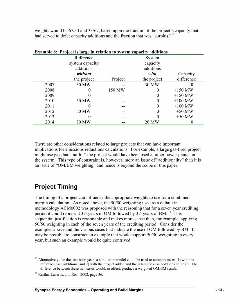
Synapse Energy Economics – Operating and Build Margins - 13 -
weights would be 67/33 and 33/67, based upon the fraction of the project’s capacity that had served to defer capacity additions and the fraction that was “surplus.”10 Example 6: Project is large in relation to system capacity additions Reference
system capacity additions without
the project
Project
System capacity additions
with the project
Capacity difference
2007 30 MW -- 30 MW 0 2008 0 150 MW 0 +150 MW 2009 0 -- 0 +150 MW 2010 50 MW -- 0 +100 MW 2011 0 -- 0 +100 MW 2012 50 MW -- 0 +50 MW 2013 0 -- 0 +50 MW 2014 70 MW -- 20 MW 0
There are other considerations related to large projects that can have important implications for emissions reductions calculations. For example, a large gas-fired project might use gas that “but for” the project would have been used at other power plants on the system. This type of constraint is, however, more an issue of “additionality” than it is an issue of “OM/BM weighting” and hence is beyond the scope of this paper.
Project Timing The timing of a project can influence the appropriate weights to use for a combined margin calculation. As noted above, the 50/50 weighting used as a default in methodology ACM0002 was proposed with the reasoning that for a seven year crediting period it could represent 3½ years of OM followed by 3½ years of BM. 11 This sequential justification is reasonable and makes more sense than, for example, applying 50/50 weighting in each of the seven years of the crediting period. Consider the examples above and the various cases that indicate the use of OM followed by BM. It may be possible to construct an example that would support 50/50 weighting in every year, but such an example would be quite contrived. 10 Alternatively, for the transition years a simulation model could be used to compare cases, 1) with the
reference case additions, and 2) with the project added and the reference case additions deferred. The difference between these two cases would, in effect, produce a weighted OM/BM result.
11 Kartha, Lazarus, and Bosi, 2002, page 36.

Synapse Energy Economics – Operating and Build Margins - 14 -
The 3½ year time lag assumption is, however, worth examining. In recommending 50/50 weights, the paper observes that 3½ years is “a reasonable lag time reflective of planning, construction, and permitting period for new power plants.”12 A recent OECD/IEA report titled Projected Costs of Generating Electricity: 2005 Update collected information on power plant construction times. It concluded that the construction times for coal units “as reflected in expense schedules, are around four years for most plants and, when they exceed four years, the expenses during the first years often are marginal.”13 The same report found that “gas-fired power plants are built rapidly and the expense schedules reported show that in most cases expenditures are spread over two to three years.”14 The assumptions used in the US government’s energy modeling are summarized in Table 1.15 These are consistent with the coal and gas numbers from the OECD/IEA report, and include lead time estimates for other electric generating technologies. An assumption of three or four years would appear to be reasonable for many fossil and renewable generating technologies. For combustion turbines (for peaking service) and photovoltaic facilities the lead time could be shorter, and for nuclear generating capacity the lead time could be longer. For construction of new hydroelectric facilities the lead time will tend to be project-specific. Table 1. Lead times for new electric capacity Technology Lead time (in years) Coal 4 Gas combined cycle 3 Combustion turbine 2 Fuel cells 3 Nuclear 6 Biomass 4 Landfill gas 3 Geothermal 4 Wind 3 Solar thermal 3 Photovoltaic 2 These figures are relevant to the weighting of OM and BM in that they can play a role in determining the point in time that OM should switch to BM for a particular project in a
12 Ibid. 13 OECD/IEA 2005, page 36. 14 Ibid, page 40. 15 EIA 2004, page 71.

Synapse Energy Economics – Operating and Build Margins - 15 -
particular system context. As with project size, it is not the absolute construction time that matters, but rather the relative construction time. Consider a project applying CDM credit today (the beginning of year one) that has not yet begun construction (since the CDM credit is critical to the project moving forward). Approval of the CDM credit takes place at the beginning of year two. At that point it will take three years to complete the construction of the project (including any remaining design and permitting). On this timeline the project begins generating electricity at the beginning of year five. If the reference case has a coal unit capacity addition scheduled for the beginning of year six and the construction lead time for that unit is four years, then it would be deferrable by CDM project. In this case the seven year project crediting period would be years numbered five through eleven of the example. In year five, an OM (100 percent) would apply and in years six though eleven, a BM (100 percent) would apply. If this were going to be credited as a single “simultaneous combination,” then the CM weights for the first crediting period would be 14/86 OM/BM. The use of construction period or lead time, excluding planning and permitting, is reasonable, since a project is reasonably likely to be cancelled prior to the granting of its permits and prior to the investment of significant amounts of capital. Units that are under construction can, of course, be cancelled (or their construction schedules stretched intentionally or unintentionally for various reasons) but this is much less common. The U.S. is currently covered with partially-completed and abandoned power plant construction projects, but this is not the normal situation, and once a large amount of capital has been spent the project developers are generally quite focused on completing the construction as soon as reasonably possible. This type of approach, involving specific consideration of the lead time of the project and the lead time of the system capacity additions, is a promising method for determining the appropriate application of weights that reflect project- and system-specific conditions. It can reflect the reality in which system capacity additions are and are not deferrable by a particular project, and it can probably be reflected in a reasonably clear and practical “new methodology” that also would be appropriate for larger CDM projects.
Implications for Time Periods beyond Seven Years The rationale in terms of timing for the 50/50 OM/BM weights has implications for the weights appropriate beyond the first seven years. Projects have the option to use a ten year crediting period instead of the seven year period discussed above. The logic of using 3½ year lead time to support the default of 50/50 weighting for a seven year crediting period would indicate that for a ten year period the analogous OM/BM weight should be 35/65 OM/BM.

Synapse Energy Economics – Operating and Build Margins - 16 -
Similarly, the logic supporting the 50/50 weights in terms of timing during the first crediting period suggests that for the second (and third) crediting periods, 100 BM should be used. In year eight of a project’s operation it will almost surely have had time to affect the capacity mix of the system. The appropriate treatment of time periods beyond seven years deserves further thought in that there may be other considerations such as sensitivity of the calculations that could influence the appropriate methodology for weighting OM and BM.
Project Operating Mode: Baseload, Intermediate, and Peaking With respect to the type of operation, systems typically have a mix that includes baseload, intermediate (or “cycling”), and peaking resources, and over a longer time period will need to add an additional mix. Still, at any particular point in time the system may be out of balance, and the near-term future additions will be dominated by a single type of resource. Consider Example 7 below in which a system that has an existing mix that is overly dependent on baseload resources such that the next capacity additions in the reference case will be peaking combustion turbines (CTs). In the reference case, after two 50 MW CT additions (in 2010 and 2012), a coal unit designed for baseload operation would be added (in 2014). In this example, there is no baseload capacity to be added to the system until 2014, so the project (a baseload resource itself) cannot displace new baseload capacity until that time. In its first two years of operation the project would add additional capacity to the system and an OM calculation would be appropriate. For years three through six, however, a mixed situation would occur. For the “mixed” years, the net system capacity difference (listed in the right-hand column of the table) would be zero, but the baseload project would have replaced peaking capacity additions. This is not strictly a build margin situation, since the project would generate considerably more electricity (kWh) than would the CT capacity that it replaced. If the CT capacity would have operated at a very low capacity factor, then the emissions reductions for those intermediate years (marked with a “*” in the table) would essentially be an operating margin calculation to estimate the effect of the baseload project’s generation displacing generation from a mix of existing system resources. If the CT capacity would have operated at a significant (but still not baseload) capacity factor, then the ideal approach would be to simulate the system with both resource mixes to quantify the mix of existing generation and generation from the CT that would be displaced. Alternatively, without running a simulation model, some weights could be devised based upon an assumption that the CT generation would be displaced first, and then the remaining project generation would displace the existing system margin according to an approved OM approach.

Synapse Energy Economics – Operating and Build Margins - 17 -
Example 7: Baseload project defers peaking capacity additions Reference system
capacity additions without
the project
Project
System capacity additions
with the project
Capacity difference
2007 30 MW -- 30 MW 0 2008 0 10 MW base 0 +10 MW 2009 0 -- 0 +10 MW 2010 50 MW CT -- 40 MW CT 0 * 2011 0 -- 0 0 * 2012 50 MW CT -- 50 MW CT 0 * 2013 0 -- 0 0 * 2014 70 MW Coal -- 10 MW CT
+ 60 MW Coal 0
In Example 7, during the transition years (2010 to 2013) the baseload project displaces a peaking addition in the reference case. The justification for the peaker was, presumably, mainly to provide capacity for system reliability rather than low cost energy. The project provides energy and capacity, thereby entirely replacing the justification for the peaking unit (capacity) and providing additional service (energy) to the grid. This example can be extended to address a situation in which a baseload project displaces peaking, then intermediate, and finally baseload system capacity additions, in turn. Consider, for example, a system that, as in the previous example, has an existing mix that is overly dependent on baseload resources, and that the next capacity additions in the reference case will be a peaking combustion turbine (CT) in 2010 followed by an intermediate CC in 2012. In the reference case, after these peaking and intermediate additions, the same coal unit designed for baseload operation would be added in 2014. In Example 8, as in Example 7, there is no baseload capacity to be added to the system until 2014, so the project (a baseload resource itself) cannot displace new baseload capacity until that time. Also, in both examples, in its first two years of operation the project would add additional capacity to the system and an OM calculation would be appropriate. Here, however, the mixed situation in years three through six could be different and more complex than that in Example 7. For the “mixed” years, the net system capacity difference (listed in the right-hand column of the table) would be zero, but the baseload project would have replaced peaking capacity additions (in years three and four) and intermediate capacity additions (in years five and six). This is not strictly a build margin situation, particularly in years three and four, in which the project displaced CT capacity that would have operated at a very low capacity factor. For those two years (marked with a “*” in the table) the displacement situation would essentially be an operating margin calculation. In years five and six (marked with “**” in the table) however, since the displaced CC capacity would have

Synapse Energy Economics – Operating and Build Margins - 18 -
operated in intermediate or cycling mode (say, at a 30 percent capacity factor) the situation is neither strictly an OM nor strictly a BM calculation. For these two years, some sort of combined margin would be appropriate. It could be quantified by comparing a pair of computer simulation model runs, or perhaps by using a simple default mix (e.g., 50/50 OM/BM). Note that the build margin portion of the mix would, in this example for years five and six, be based upon a new gas CC rather than the new coal addition that could not be displaced until the year it would have appeared in the reference case, 2014. Example 8: Baseload project defers peaking and intermediate capacity additions Reference
system capacity additions without
the project
Project
System capacity additions
with the project
Capacity difference
2007 30 MW -- 30 MW 0 2008 0 10 MW base 0 +10 MW 2009 0 -- 0 +10 MW 2010 50 MW CT -- 40 MW CT 0 * 2011 0 -- 0 0 * 2012 50 MW CC -- 10 MW CT
+ 40 MW CC 0 **
2013 0 -- 0 0 ** 2014 70 MW Coal -- 60 MW Coal 0
In both Examples 6 and 7 above, a baseload project was being evaluated in the context of a system whose first reference case addition was to be a peaking capacity (a CT). The reverse mismatch of operating modes is also worth consideration. That is, take the example of a low capacity factor project being added to a system in which the next reference case capacity addition is expected to be a baseload coal unit. This is depicted in Example 9.

Synapse Energy Economics – Operating and Build Margins - 19 -
Example 9: Intermediate project defers baseload capacity addition Reference
system capacity additions without
the project
Project
System capacity additions
with the project
Capacity difference
2007 30 MW -- 30 MW 0 2008 0 10 MW int 0 +10 MW 2009 0 -- 0 +10 MW 2010 10 MW Coal -- 0 0 * 2011 0 -- 0 0 * 2012 10 MW Coal -- 10 MW Coal 0 * 2013 0 -- 0 0 * 2014 10 MW CC -- 10 MW Coal 0
For this example, consider a 10 MW gas-fired project expected to operate at a capacity factor of 30 percent. This project is to be added to a system with 10 MW baseload coal units to be added in 2010 and 2012, followed by an intermediate mode 10 MW CC in 2014. The current system may be out of balance with too much peaking capacity, so that some baseload additions are needed in order to bring the system into balance with an economical mix of capacity of different operating modes. For this system, there are at least two different effects that the 10 MW intermediate project could have. If may defer the coal capacity addition or it may supplement the coal. These two possibilities are illustrated in Examples 9 and 10, respectively. In Example 9 the intermediate project defers the 10 MW reference case coal addition in 2010, effectively pushing the entire series of reference case capacity additions out in time two years. In this example, the emissions reduction quantification for the first two years of the project’s operation (2008 and 2009) would be a straightforward operating margin calculation. For the third through sixth year of project operation (2010 to 2013) the emissions reduction calculation would, at least conceptually, be a complex mix reflecting the fact (in this example) that the deferred coal capacity would have had a higher capacity factor than the project itself. The relevant calculation would be as follows:
emissions reduction = coal unit emissions – (project emissions + S) where S is the additional emissions from the existing system power plants resulting from the lost generation. This lost generation is the amount of energy that would have been produced at the coal unit and was not replaced by energy generation from the project. In other words, the displaced coal unit would have operated more than the project itself, and this difference in generation (and associated emissions) must be made up by the existing system resources. In Example 9, a project with an intermediate mode of operation (e.g., 30 percent capacity factor) displaced a baseload coal capacity addition that would have occurred in the

Synapse Energy Economics – Operating and Build Margins - 20 -
reference case, but for the project. This would only occur if the economic justification of the reference case coal addition depended upon the capacity or system reliability value of that coal addition. One can image a different situation in which the reference case coal addition is economically justified entirely on the basis of its low cost energy.16 If this were the case, then the 10 MW intermediate project would not displace the coal unit, but rather would supplement it. The emissions reduction calculation for years three through six in the example would then be a 100 percent operating margin calculation. This is depicted in Example 10. Example 10: Intermediate project supplements baseload capacity addition Reference
system capacity additions without
the project
Project
System capacity additions
with the project
Capacity difference
2007 30 MW -- 30 MW 0 2008 0 10 MW int 0 +10 MW 2009 0 -- 0 +10 MW 2010 10 MW Coal -- 10 MW Coal +10 MW * 2011 0 -- 0 +10 MW * 2012 10 MW Coal -- 10 MW Coal +10 MW * 2013 0 -- 0 +10 MW * 2014 10 MW CC -- 0 0
Examples 9 and 10 differ greatly in terms of what is displaced in the transition years (2010 to 2013). In the first case, the 10 MW project defers a 10 MW baseload capacity addition that would have generated more energy than the project itself. In the second case, the 10 MW project defers nothing (except operating margin). Hybrid situations, in which some combination of the two situations would occur, are also possible. Indeed, the many possibilities and the difficulty of determining in any particular practical context which is the “right” way to estimate the impact of the project on the system can be daunting for the analyst. The complexity also presents quite a challenge for one wishing to draft methodology language to implement this sort of mixing of resource types in a way that would be reasonably appropriate to all projects and contexts. There are, however, some general principles that may be gleaned from these examples and applied in emissions reduction calculations. Specifically:
16 By definition “baseload resources” have high construction costs and low operating costs, while “peaking
resources” have low construction costs and high operating costs. Low and high are, of course, relative terms. And “intermediate resources” would fall somewhere between baseload and peaking in terms of construction and operating costs.

Synapse Energy Economics – Operating and Build Margins - 21 -
1. With regard to different operating modes, the project can be expected at some point in time to displace a reference case capacity addition that resembles the project. That is, a baseload project will eventually displace (100 percent) a “baseload build margin” and a peaking project will eventually displace (100 percent) a “peaking build market.”
2. What happens in the transition years logically can depend upon the justification
for the reference case capacity additions (which do not match the project in terms of operating mode).
Note that the types of situations discussed above, in which a project defers a sequential series of different reference case capacity types, could arise in other contexts. For example, if instead of the mode of operation, the reference case has system capacity additions of various types that are scheduled to be built in an alternating sequence. This is examined in more detail in the following section.
Reference Case Mix of Capacity Types It is common for a reference case system plan to include more than one type of capacity addition. In the examples discussed above (Examples 7 through 10), the reference case has capacity of different operating modes, which might be displaced in a logical sequence depending upon how they compare with the operating mode of the project. A different situation could involve reference case capacity additions that vary for other reasons. Considerations of resource diversity, for example, could result in a reference case system expansion plan in which two new resource types alternate. Example 11 shows a situation with alternating coal and hydro additions in the reference case.
Example 11: Reference case with alternating capacity additions Reference
system capacity additions without
the project
Project
System capacity additions
with the project
Capacity difference
2007 30 MW -- 30 MW 0 2008 0 10 MW 0 +10 MW 2009 0 -- 0 +10 MW 2010 10 MW coal -- 0 0 2011 10 MW hydro -- 10 MW coal 0 2012 10 MW coal -- 10 MW hydro 0 2013 10 MW hydro -- 10 MW coal 0 2014 10 MW coal -- 10 MW hydro 0

Synapse Energy Economics – Operating and Build Margins - 22 -
Here the project is assumed to simply shift the reference case plan by one year. The capacity differences are, after the first deferral in 2010, zero. Prior to this point, a 100 percent OM calculation would be appropriate. After this point, a 100 percent BM calculation would be appropriate. However, because the new capacity type was alternating in the reference case, the capacity type for the build margin calculation would also alternate. In 2010 the project displaced a coal unit. In 2011, the coal addition is in both cases and the project displaced a hydro unit. And so on. In actual situations it would likely be impractical to determine with such precision what the year-by-year effect of a project on this sort of system would be. A methodology in which the system additions were “blended” (either on an ex-ante or ex-post basis) would seem sensible. The blending could reflect the fact that reference case additions are of two (or more) types without pretending to know more about the effect of the project than can reasonably be determined.
System Capacity Surplus and Shortage The state of the electric power system in terms of overall capacity excess or shortage can have a bearing on the calculation of displaced emissions from the grid, and in particular upon the role of OM and BM in those calculations. In Example 6, above, we considered a situation in which a large project (relative to the size of the system) was added, shifting the system into a capacity surplus situation for some time (for six years in the example). A capacity surplus can also arise prior to and separate from a particular project. Specifically, after the addition of a large generating unit (or set of units) a system may be in a surplus state. This can also be caused or exacerbated by slower-than-forecast demand growth or, in extreme cases, by absolute declines in system demand. Where a large capacity surplus exists, it will tend to push the first reference case capacity addition out in time. This in turn will increase the importance of the OM and diminish the role of the BM in determining the system impact of a project. It could be the case, for example, that the system does not have any new capacity planned for the entire first crediting period of a project, and so no capacity can be deferred by the project and a 100 percent OM calculation would be appropriate in that crediting period. This treatment of surplus situations is conceptually quite straightforward. There are factors that potentially make it complicated in practice. For example, there is likely to be uncertainty about the level of future demand growth and whether no new capacity additions would, in fact, be made in the reference case over a particular period of time. Relative to other complications, however, this is not particularly difficult to deal with. The uncertainty in this case can be addressed by the use of best available projections and/or ex-post analysis.

Synapse Energy Economics – Operating and Build Margins - 23 -
The implications of a system capacity shortage situation upon emissions reduction calculations depend upon the nature of the shortage. If there is a temporary capacity shortfall on a system that is normally in reasonable balance then this would simply move up the point in time at which 100 BM would be appropriate to attribute to a project. That is, the reference case system capacity expansion scenario would, for a system temporarily short on capacity, likely include significant deferrable capacity additions early in the crediting period. If the capacity shortage is chronic, however, then different logic and different considerations prevail. Specifically, in a system that is always attempting to add capacity to meet growing demands and falling short of a reasonable balance of supply with demand, it is not clear how the principles illustrated in the many examples above would apply. Is a system that is adding capacity but always short, a situation in which the project would nonetheless displace a portion of that new capacity (and BM would tend to apply) or one in which the project is entirely incremental to those reference case additions (and OM would tend to apply)? These issues are tightly intertwined with issues of fairness to countries that are addressed in the recent Marrakech Accords and extend beyond the technical issues that are the focus of this paper.
Project Characteristics: Intermittency and Seasonality Some projects have generation patterns that are intermittent or seasonally dependant, and do not fit the conventional categories of baseload, intermediate, or peaking operation. These raise a special set of issues to address in quantifying emissions reductions and in applying OM, BM, and CM methods. Wind generating capacity is an example of a resource with intermittent operation. Consider a wind generator with an installed capacity rating that operates at a 30 percent capacity factor. If this wind project is added to the system it will not displace 100 MW of new reference case baseload capacity. Some may argue that the wind project is not firm and will displace zero reference case capacity, and so a 100 percent OM approach should be used. It would be more reasonable, assuming that the wind generation pattern is random throughout the year and that the amount of wind capacity is small relative to the total electric system, to assume that the wind project would displace about 30 MW of reference case capacity. If the system is centrally planned, then this is roughly the “capacity credit” that planners could credit to the wind project. In a market-based system, the wind project would tend to have an effect on market prices similar to that amount of baseload capacity, and so would have a similar magnitude effect upon the capacity additions that project developers would economically justify. The calculation for this wind project would be similar to the various examples discussed above, but the capacity rating used for the OM and BM calculation would resemble the average capacity of the facility rather than the installed capacity. The average capacity could be calculated as the installed capacity rating multiplied by the capacity factor.
Synapse Energy Economics – Operating and Build Margins - 24 -
Two conditions stated in the example above are related to the amount of intermittent capacity on the grid and the timing of the generation from the intermittent project. With regard to the amount, so long as the intermittent generation is less than approximately 10 percent of the total system capacity, then the relationships should apply reasonably well. At higher levels of intermittent generation, particularly if the intermittent generation is all from one facility (or from facilities with generation patterns that are highly correlated to each other), then the capacity value of each additional increment of intermittent generation added to the system will be decreased. At some point the amount of intermittent generation on the system may be so high that any additional intermittent capacity has no value to the system whatsoever, and a 100 percent OM approach would be appropriate. Few, if any, electric systems in the world are at or near this point. The timing of the intermittent generation can have an important impact upon the capacity value of a project to the system, and so upon the OM/BM mix to apply in a particular case. If, for example, a wind project has most of its generation produced during the nighttime or during seasons of the year with low demand, then the capacity value of the wind project will tend to be lower than that of the “randomly distributed” wind project discussed above. In an extreme case, with all of its generation produced in off-peak load periods, the capacity value of a project could be zero. This timing issue, for wind projects, tends to be highly specific to locations. There are places where the wind correlates positively with system loads and the capacity value appropriate to attribute to a project would be greater than the average capacity. There are places where the wind correlates negatively with system loads (e.g., most of the strong wind blows in the winter but the system is summer peaking) and the capacity value appropriate to attribute to a project would be less than the average capacity. There are places where there is no correlation, positive or negative, between the pattern of wind generation and loads, and the average capacity assumption would be reasonable. This is project and location specific in such a way that it would be difficult to specify a general methodology that would apply well to all cases. Perhaps it would be reasonable to use the average capacity assumption unless there is data to support deviation. In a case where a wind project with 100 MW installed capacity and 30 MW average capacity were known to have less than 30 MW of capacity value, the OM/BM combination could be applied along the lines of Example 7, above. The wind project would have more generation than would the capacity that it displaced, and that additional generation should be accounted for in the emissions reduction calculation (either by system modeling or by a rough weighting of OM and BM). Hydroelectric projects can have generation patterns that should be considered in quantifying displaced emissions. These can be similar to the seasonal patterns discussed above for wind. Rainfall patterns in particular locations are only rarely level throughout the year. Moreover, in places where the hydro plants depend upon snow melt for water, there can be a distinct seasonality to the generation. If a system has its peak demands in the summer and a hydro project has most of its generation in the spring (due to rainfall

Synapse Energy Economics – Operating and Build Margins - 25 -
and snow melt patterns), then conceivably that hydro project could have little or no value for deferring system capacity. That would, however, be an extreme case. More likely, the hydro project would have some generation available in the summer (or whenever the system peak demands occur) and would defer system capacity additions, thereby deserving some capacity value. Also, a hydro project may have some ability to store water on a daily basis so that even if it cannot generate at a high capacity factor during the summer, it may still be able to run at or near17 its full installed capacity rating for a few hours during the system peak periods, thereby providing nearly full capacity value, displacing reference case capacity additions one-for-one, and deserving a 100 percent BM for purposes of emissions displacement calculations.
Existing Hydro System In addition to the considerations related to wind and hydro projects on an individual basis (discussed in the previous section) there are interesting interactive effects of intermittent resources (e.g., wind) and storage resources (e.g., hydro) operating on the same system. These are part of a larger set of issues of calculating displaced emissions on hydro systems. Hydro system operation can be extremely complex, subject to myriad constraints related to the weather, storage capability, various human and ecological uses of the rivers and reservoirs, the physical relationships among the hydro facilities (some are downstream from, and so influenced by, other upstream facilities), and other factors. Generally, some sort of optimization is done to dispatch a set of hydro facilities, or optimization analysis is done to develop operating rules that are used to dispatch the facilities. Because these rules can be detailed and complex, and because there are computer models in existence to simulate these systems, there is a quite understandable inclination to use those models in calculating displaced emissions for projects on such systems. This can, however, be an extreme example of the “black box” model being applied in a situation in which it is not well understood or applicable. For example, if a project is being added to a hydro-dominated existing system, the wish to represent the intricacies of the hydro system dispatch optimization in the emissions calculation for the project might inadvertently cause one to use a 100 percent OM calculation approach, even if that were not appropriate in the circumstances. For an OM calculation on a hydro-dominated system, a simulation model might be quite reasonable. Consider, for example, the first two years of project operation (2008 and 2009) in Example 1. If that were on a hydro system, then the OM would apply in those years, and it could be quantified in a number of ways. However, in 2010 and beyond, if the baseload project defers an equivalent amount of new baseload fossil-fuel capacity that
17 The capability of the unit may be reduced slightly, say by a few percent, as a result of the lower reservoir
levels and correspondingly lower head.
Synapse Energy Economics – Operating and Build Margins - 26 -
would have been built in the reference case, then the OM would no longer apply and the complex hydro dispatch simulation would no longer be relevant. System simulation models can be quite useful in performing emissions reductions calculations for electric power systems. There are many models available, each with its strengths and weaknesses. Several models and their application to emissions displacement calculations are reviewed in Predicting Avoided Emissions from Policies that Encourage Energy Efficiency and Clean Power and Estimating the Emission Reduction Benefits of Renewable Electricity and Energy Efficiency in North America: Experience and Methods. In all cases, the models offer the possibility of adding detail and technical rigor to the analysis while at the same time creating some risk of misuse and the “black box” problem of lack of transparency. Systems that are truly dominated by storage hydro facilities can be “energy limited” rather than “capacity limited” in terms of system expansion. Where this is the case, some of the normal considerations in thermal systems would not apply. For example, the need of the system to meet an annual peak hour demand may be essentially irrelevant, and the plan for new capacity additions to the system driven entirely by the amount of energy that those resources produce, rather than their capacity ratings. In these energy-limited cases, some things are more straightforward than they might be on a thermal capacity-limited system. For example, an intermittent wind project might displace reference case capacity entirely on the basis of the amount of energy produced over the course of a year, and the hour-to-hour, or even seasonal, fluctuations are of no consequence.
Grid System Management Electricity systems around the world are owned and operated subject to different mixes of market and regulatory forces. While these differences have dramatic implications for prices and other significant impacts, the relevance to determination of weights for operating and build margins is quite minor. In any case, the dispatch of a grid will be administered by some central entity. Where economic regulation dominates, the system dispatch will be based upon estimated marginal costs of each generating unit. Where electricity markets have been deregulated, the central dispatch will be based mainly upon supply offers from generators. The difference between marginal cost-based dispatch and bid-based dispatch should be quite minor in terms of its impact upon the relative place of different resources in the merit order, and hence upon the mix of what would be displaced in an OM calculation. Likewise, with regard to capacity additions, there is little conceptual difference in terms of the timing and mechanisms for BM calculations. In a centrally planned system the schedule and type of capacity additions will be determined by planners running models and analyzing resource options. Those planners will work with objectives and constraints

Synapse Energy Economics – Operating and Build Margins - 27 -
that reflect economics,18 system reliability requirements, environmental impacts and regulations, and political factors. In a market system the schedule and type of capacity additions will be determined by companies attempting to maximize their profits and minimize their risk exposure. These companies operate in a context of economics, system reliability requirements, environmental impacts and regulations, and political factors that is not dissimilar from that of the regulated context. Indeed, anywhere in the world, the electric grid is subject to a combination of regulatory/political and market/economic forces. Within a regulated system, resources will be added based at least partly upon their projected costs and benefits where the benefits are determined by the value of the fuel and capital that they displace on the grid. Within a market system, resource decisions will be driven, at least in part, based upon market prices for electricity at particular times and locations. Those prices should resemble the value of marginal fuel and capital. If they do not, over the long-term this would indicate a problem. There may be some differences between the regulated and market contexts. For example, the reference case resource plans may emphasize different types of generating technologies and fuels. However, the approaches to use in estimating OM and BM effects and in weighting CM calculations for CDM credit should not differ greatly.
Conclusions: Guidance for Project Developers and Topics for Further Research The concepts discussed in this paper have implications for what is and is not reasonable for methodologies for quantifying carbon emissions reduction credit and for the application of those methodologies to particular projects in specific system contexts.
1. The 50/50 OM/BM default appears broadly reasonable and should be acceptable for many projects, particularly smaller projects for which the rigor of a more detailed examination would be unduly burdensome.
2. Small project size is not generally a legitimate reason for increasing the OM portion of an emissions reduction calculation.
3. The relative timing of the system’s first deferrable new capacity addition (relative to the timing of the project) could be a legitimate reason for deviating from the 50/50 default weights in either direction. For example, if the first deferrable system capacity addition is expected to occur prior to halfway through the first crediting period, then that would indicate placing a greater weight on the BM.
18 Economic factors include the capital and operating costs of different resources, and access to capital.

Synapse Energy Economics – Operating and Build Margins - 28 -
4. System simulation models can have a useful role in the displaced emissions calculations, particularly for larger projects (where the burden is relatively less and the benefit of increased accuracy is relatively greater). The increased detail and rigor available with simulation modeling should not, however, come at the expense of reasonable weighting of OM and BM. For example, because the simulation models tend to focus on operations, they might tend to emphasize OM, even for years in which BM is the appropriate basis for the calculation.
5. New system capacity additions that are included in both the reference case and in the project case do not represent BM in the emission reduction calculation if they have the same timing and characteristics in both cases. If they are deferred by the project or caused to be smaller as a result of the project, then they would be contributing directly to the BM.
6. Project characteristics such as intermittency or seasonality in generation patterns can legitimately have some bearing on the OM/BM weights. For example, if the generation from a resource tends to be produced during off-peak periods such as nights or shoulder seasons, that could tend to increase the weight appropriate for OM. In general, however, in the absence of information about whether generation patterns are positively or negatively correlated with loads, a “MWh-for-MWh” displacement assumption should be used.
7. If a system is in a significantly surplus state, this can legitimately influence the OM/BM weights appropriate to a project, increasing the weight to be placed upon OM. The proper way to reflect that in the calculation is to examine the date of the first deferrable system capacity addition in the reference case and use OM/BM weights that reflect that timing, relative to the crediting period for the project.
8. The type of grid system management (the mix of planning, regulation, and market forces) does not have an obvious implication for the weighting of OM and BM in emission reduction calculations, as the fundamental underlying drivers of system capacity additions will be at work regardless.
In any specific situation, characteristics of the project and/or the electric system will have a bearing upon the impact of a project upon the system operation and expansion. In some cases, there are likely to be complex or unusual effects that could not be anticipated in a general methodology. In those cases, the conceptual framework developed in this paper might serve as a guide to how those project-specific or system-specific features should be accounted for in computing the OM and BM, and in combining the two.
This paper represents an attempt to develop a conceptual framework for methodologies that apply or combine operating and build margins. Useful next steps for research along these lines could include:

Synapse Energy Economics – Operating and Build Margins - 29 -
1. investigation of how well (or poorly) online dates for new capacity projects are forecasted;
2. drafting methodology language to incorporate timing issues (project relative to system capacity additions) in calculating the baseline emission factor for a project;
3. development of methodologies that blend two or more types of reference case capacity additions into a build margin (either on an ex-anti or ex-post basis);
4. further consideration of specific project characteristics such as intermittency and seasonality of generation;
5. further consideration of grid surplus and shortage conditions;
6. consideration of the factors that influence the appropriate methodology for ten year crediting periods and for subsequent seven year periods; and
7. development of further examples to illustrate and understand the concepts that govern the impact of a project upon an electric system’s capacity additions, perhaps combining some of the issues that are taken up here individually.

Synapse Energy Economics – Operating and Build Margins - 30 -
References Biewald, Bruce, and Geoff Keith. 2004. “Estimating Emission Reductions from Energy Efficiency in the Northeast,” in Proceedings: 2004 ACEEE Summer Study on Energy Efficiency in Buildings. American Council for an Energy-Efficient Economy.
Kartha S., M. Lazarus, and M. Bosi. 2002. Practical Baseline Recommendations for Greenhouse Gas Mitigation Projects in the Electric Power Sector. Paris: OECD and IEA. www.ghgprotocol.org/docs/Electric_Power_Sector_Baselines.pdf.
Keith, G., B. Biewald, A. Sommer, P. Henn, and M. Breceda. 2003. Estimating the Emission Reduction Benefits of Renewable Electricity and Energy Efficiency in North America: Experience and Methods. Prepared for the Commission for Environmental Cooperation.
Keith, Geoff, and Bruce Biewald. 2002. Predicting Avoided Emissions from Policies that Encourage Energy Efficiency and Clean Power. Prepared for the Ozone Transport Commission.
Marnay C., D. Fisher, S. Murtishaw, A. Phadke, L. Price, and J. Sathaye. 2002. Estimating Carbon Dioxide Emissions Factors for the California Electric Power Sector. Berkeley: Lawrence Berkeley National Laboratory. http://eetd.lbl.gov/ea/EMS/reports/49945.pdf.
Matsuo, Naoki. 2004. CDM Methodologies Guidebook. Japan: Ministry of the Environment (MOE), Global Environment Centre Foundation (GEC), Climate Experts Ltd.. http://gec.jp/gec/gec.nsf/en/Publications-Reports_and_Related_Books-CDM_Meth_Guidebook.
Organisation for Economic Co-operation and Development. International Energy Agency. 2000. Emission Baselines: Estimating the Unknown. Paris: OECD. www.iea.org/textbase/nppdf/free/2000/embase2000.pdf.
Organisation for Economic Co-operation and Development. Nuclear Energy Agency. International Energy Agency. 2005. Projected Costs of Generating Electricity: 2005 Update. Paris: OECD/IEA.

Synapse Energy Economics – Operating and Build Margins - 31 -
United Nations. United Nations Framework Convention on Climate Change. 1992. Kyoto Protocol to the United Nations Framework Convention on Climate Change. http://unfccc.int/resource/docs/convkp/kpeng.html.
United Nations. Clean Development Mechanism Executive Board. 2004. Approved Consolidated Baseline Methodology ACM0002: Consolidated baseline methodology for grid-connected electricity generation from renewable sources. Version 2. http://cdm.unfccc.int/UserManagement/FileStorage/ACM0002_Consolidated_elct_version_2.pdf.
United Nations. Clean Development Mechanism Executive Board. 2004. Consolidated Methodology for Grid-connected Electricity Generation from Renewable Sources, Version 2. United Nations Framework Convention on Climate Change (UNFCCC). http://cdm.unfccc.int/UserManagement/FileStorage/ACM0002_Consolidated_elct_version_2.pdf.
United States. Energy Information Administration. 2004. Assumptions for the Annual Energy Outlook 2004 with Projections to 2025. United States Department of Energy.