Using Different Many-Objective Techniques inParticle Swarm Optimization for Many Objective

Problems: An Empirical StudyAndre B. de Carvalho and Aurora Pozo

Computer Science Department, Federal University of Parana,Cel. Francisco H. dos Santos Street, Centro Politecnico, Curitiba, PR, Brazil

andrebc, aurora@inf.ufpr.br

Abstract:Pareto based Multi-Objective Evolutionary Algorithms faceseveral problems when dealing with a large number of ob-jectives. In this situation, almost all solutions become non-dominated and there is no pressure towards the Pareto Front.The use of Particle Swarm Optimization algorithm (PSO) inmulti-objective problems grew in recent years. The PSO hasbeen found very efficient in solve Multi-Objective Problems(MOPs) and several Multi-Objective Particle Swarm Optimiza-tion algorithms (MOPSO) have been proposed. This work hasthe goal to study how PSO is affected when dealing with Many-Objective Problems. Recently, some many-objective techniqueshave been proposed to avoid the deterioration of the searchability of multi-objective algorithms. Here, two many-objectivetechniques are applied in PSO: Controlling the DominanceArea of Solutions and Average Ranking. An empirical analysisis performed to identify the influence of these techniques on con-vergence and diversity of the MOPSO search in different many-objective scenarios. The experimental results are analyzed ap-plying some quality indicators and some statistical tests.Keywords: Many-Objective Optimization, Multi-Objective Opt-mization, Particle Swarm Optmization

I. Introduction

Particle Swarm Optimization (PSO) [18] is a populationbased meta-heuristic that has been used to solve several op-timization problems [24]. PSO algorithms are inspired onanimal swarm intelligence and are based on the coopera-tion of the individuals. Multi-objective optimization prob-lems (MOPs) are usually solved by a large number of multi-objective evolutionary algorithms (MOEAs) [19], includ-ing PSO. However, several problems arise when dealingwith a large number of objectives. Problems with morethan three objectives are called Many-Objective Problems(MaOPs) [14]. The main obstacle faced by MOEAs in many-objective is the deterioration of the search ability, becausealmost all solutions are non-dominated there is no pressuretowards the Pareto Front.To overcome these limitations, in recent years the interest forMany-Objective Optimization has grown [14] [25]. In thisarea, some techniques have been proposed like Controllingof Dominance Area of Solutions (CDAS) [26] and the use of

rankings [17], like Average Ranking [3]. The goal of theseworks is to study techniques that decrease the negative effectsof using several objectives.The paper [9] presented a first study on the influence ofthe CDAS technique in PSO for Many-Objective Problems(MaOPs). The main idea of the paper was to observe the in-fluence of controlling the dominance area of solutions on as-pects like convergence and diversity in a metaheuristic basedon cooperation between individuals. Here, this work presentsan extension of the use of many-objective techniques in Par-ticle Swarm Optimization. We extend the previous study byapplying a different many-objective technique, called the Av-erage Ranking (AR) [3]. This technique induces a preferenceordering over a set of solutions, and then a MOPSO algo-rithm chose the best solutions through this preference order,instead of, dominance relation.We perform an empirical analysis to measure the perfor-mance of MOPSO in Many-Objective problems using thesetwo preference relations: CDAS and AR. The chosen algo-rithm is the SMPSO [22], and two extended algorithms areimplemented CDAS-SMPSO [9] and AR-SMPSO. These al-gorithms are applied to two benchmark many-objective prob-lems, DTLZ2 and DTLZ4 [11]. A set of quality indicators isused to investigate how these techniques affect convergenceand diversity of MOPSO search in many objective scenar-ios : Generational Distance (GD), Inverse Generational Dis-tance (IGD), Spacing and also it is analyzed the distributionof the Tchebycheff distance over the ”knee” of the Paretofront [15].The rest of this paper is organized as follows: Section IIpresents the main concepts of many-objective optimizationand Section III discusses some related works. In Section IVthe previous work that uses CDAS in SMPSO is revised. Af-ter, Section V describes the use of AR in the SMPSO al-gorithm. Finally, Section VI presents empirical experimentsand Section VII discusses the conclusions and future works.

II. Multi-Objective Optimization

Real world problems usually include multiple criteria thatshould be satisfied at the same time. Furthermore, in such

International Journal of Computer Information Systems and Industrial Management Applications ISSN 2150-7988 Volume 3 (2011) pp.096-107© MIR Labs, www.mirlabs.net/ijcisim/index.html

Dynamic Publishers, Inc., USA

problems, the objectives (or criteria) to be optimized are usu-ally in conflict, i.e. trying to improve one of them will resultin worse values for some other. For example, most decisionmaker is faced with a difficult decision problem; they wantto assure a great level of reliability and also a minimum cost.In this case, the goal is to find a good ”trade-off” of solutionsthat represent the better compromise among the objectives.The general multi-objective maximization problem (MOP)can be stated as in (1).

Maximizef(x) = (f1(x), f2(x)..., fm(x)) (1)

subject to x ∈ Ωwhere: x ∈ Ω is a feasible solution vector, Ω is the feasibleregion delimited by the constraints of the problem, and m isthe number of objectives.Important concepts used in determining a set of solutions formultiobjective optimization problems are dominance, Paretooptimality, Pareto set and Pareto front. Pareto Dominance(PD) was proposed by Vilfredo Pareto [23] and is definedas follows: given two solutions x ∈ Ω and y ∈ Ω, for amaximization problem, the solution x dominates y if

∀i ∈ 1, 2, ...,m : fi(x) ≥ fi(y), and∃i ∈ 1, 2, ...,m : fi(x) > fi(y)

x is a non-dominated solution if there is no solution y thatdominates x.The goal is to discover solutions that are not dominated byany other in the objective space. A set of non-dominatedsolutions is called Pareto optimal and the set of all non-dominated objective vectors is called Pareto front. ThePareto optimal set is helpful for real problems, e.g., engi-neering problems, and provides valuable information aboutthe underlying problem. In most applications, the searchfor the Pareto optimal is NP-hard and then the optimizationproblem focuses on finding an approximation set, as close aspossible to the Pareto optimal. Multi-Objective EvolutionaryAlgorithms have been successfully applied to many MOPs.MOEAs are particularly suitable for this task because theyevolve simultaneously a population of potential solutions tothe problem obtaining a set of solutions to approximate thePareto front in a single run of the algorithm.

III. Related Work

In a scalar objective optimization problem, all the solutioncan be compared based on their objective function values andthe task of a scalar objective evolutionary algorithm is to findone single solution. However, in MOP, domination does notdefine a complete ordering among the solutions. Therefore,MOEAs modify Evolutionary Algorithms (EAs) [6] [13] intwo ways: they incorporate a selection mechanism basedon Pareto optimality, and they adopt a diversity preservationmechanism that avoids the convergence to a single solution.Although, most of the studies on MOPs have been focusedon problems with a few numbers of objectives, practical opti-mization problems involve a large number of criteria. There-fore, research efforts have been oriented to investigate thescalability of these algorithms with respect to the number ofobjectives [14]. MOPs having more than 3 objectives arereferred as many-objective optimization problems in the spe-cialized literature. Several studies have proved that MOEAs

scale poor in many-objective optimization problems. Themain reason for this is that the proportion of non-dominatedsolutions in a population increases exponentially with thenumber of objectives. As consequence: The search ability isdeteriorated because it is no possible to impose preferencesfor selection purposes; The number of solutions required forapproximating the entire Pareto front also increases, and dif-ficulty of the visualization of solutions.Currently, the research community has been tackled these is-sues using mainly three approaches:

• Adaptation of preference relations that induce a finerorder on the objective space [26], [1], [11], [17],[15], [25], [7],.

• The dimensionality reduction is also an alternativefor dealing with the challenges of many objec-tives [21], [5], [16],[4]. The overall idea of this ap-proach is to identify the least non conflicting objectives(one that can be removed without changing the Paretooptimal set) to discard them, for instance, dismissingobjectives that are highly correlated with others.

• Decomposition strategies that uses decompositionmethods, which have been studied in the mathematicalprogramming community, into evolutionary algorithmsfor multi-objective optimization. This approach decom-poses the MOP into a number of scalar optimizationproblems, and then, evolutionary algorithms are appliedto optimize these sub problems simultaneously [28], [2].

In sum, these works reflect the focus of the current researchwhen dealing with many-objective optimization problems(MaOPs). One of the main conclusions of these works is re-lated to the weakness of the Pareto dominance relation fordealing with MaOPs and some alternative were proposed.Some authors point out that by using an effective rankingscheme, it is possible for MOEAs to converge in MaOPs.But, the ranking method must provide a fine grained discrim-ination between solutions. On the other hand, a high selec-tion pressure sacrifices diversity and the algorithm convergesto a small region.So, there exist many difficulties waiting to overcome and mo-tivate our work. One of them is related to the metaheuristic,until relatively recently, most of the research had concen-trated on a small group of algorithms, often the NSGA-II.In this work, the behavior of the Particle Swarm Optimiza-tion in MaOPs is investigated. Two previous works deal withMaOPs using PSO algorithms.In [27], it is presented an approach that uses a distance metricbased on user-preferences to efficiently find solutions. In thework, the user defines good regions on the objective spacethat must be explored by the algorithm. So, PSO is usedas a baseline, and the particles update their position and ve-locity according to their closeness to the preference regions.In this method, the PSO algorithm does not rely on Paretodominance comparisons to find solutions. The algorithm wascompared to a user-preference based PSO algorithm that usesPareto dominance comparisons to select the leaders. The re-sults showed that the algorithm obtain better results, espe-cially for problems with high number of objectives. In [20] aPSO algorithm handles with many-objectives using a Grad-ual Pareto dominance relation to overcome the problem of

Carvalho and Pozo097

finding non-dominated solutions when the number of objec-tives grows.As explained before, one of the alternative to deal withMaOPs is to use an effective ranking scheme, however, theseranking schemes have never been object of study with PSO.Then, differently of the previous many-objective PSO works,our work has the goal to study the behavior of preference re-lations in Multi-Objective Particle Swarm algorithm, a topicfew explored in the literature. The selected technique wasthe Control of Dominance Area of Solutions (CDAS) [26],and it was first applied to PSO in [9]. Here we extend thisprevious work and we apply other many-objective techniqueto PSO, the Average Ranking. The two techniques are alsocompared in different many-objective situations.

IV. Previous Work

This Section reviews our previous work [9] that had the goalto apply the control of dominance area technique (CDAS)into PSO algorithm. First, the CDAS technique is describedand its application into PSO algorithm. Finally, some resultsare discussed.Sato et al. propose a method to control the dominance areaof solutions to induce an appropriate ranking of the solutions.The proposed method controls the degree of contraction andexpansion of the dominance area of solutions using a user-defined parameter Si. The dominance relation changes withthis contraction or expansion, and solutions that were origi-nally non-dominated become dominated by others. The mod-ification of the dominance area is defined by the Equation (2):

f ′i(x) =r · sin(ωi − Siπ)

sin(Siπ)(2)

where x is a solution in the search space, f(x) is the objectivevector and r is the norm of f(x). ωi is the degree betweenfi(x) and f(x). If Si = 0.5 then f ′i(x) = fi(x) and there isno modification in the dominance relation. If Si < 0.5 thenf ′i(x) > fi(x), so will be produced a subset of the ParetoFront. In the other hand, if Si > 0.5 then f ′i(x) < fi(x)and the dominance relation is relaxed, so solutions that werenormally dominated become non-dominated.PSO is a population-based heuristic inspired by the social be-havior of bird flocking aiming to find food [18]. In PSO, thesystem initializes with a set of solutions and search for op-tima by updating generations. The set of possible solutionsis a set of particles, called swarm, which moves in the searchspace, in a cooperative search procedure. These moves areperformed by an operator that has a local and a social compo-nent. This operator is called velocity of a particle and movesit through an n-dimensional space based on the best positionsof their neighbors (social component), the leader, and ontheir own best position (local component). The best particlesare found based on the fitness function. There are many fit-ness functions in Multi-objective Particle Swarm Optimiza-tion (MOPSO). Based on Pareto dominance concepts, eachparticle of the swarm could have different leaders, but onlyone may be selected to update the velocity. This set of lead-ers is stored in an external repository (archive) [18], whichcontains the best non-dominated solutions found so far.The chosen MOPSO algorithm was the SMPSO. TheSMPSO algorithm was presented in [22]. In this algorithm,

Figure. 1: Influence of the CDAS in MOPSO leader’schoice.

the velocity of the particle is limited by a constriction fac-tor χ. The SMPSO introduces a mechanism that bound theaccumulated velocity of each variable j (in each particle).Besides, after the velocity update of each particle a mutationoperation is applied. It is applied a polynomial mutation in15% of the population, randomly selected. In the SMPSO,the archive of the leaders has a maximum size, defined by auser parameter. When this archive becomes full, the crowdeddistance is used [22] to define which particles will remain inthe repository. The choice of the leader is defined by a binarytournament.In MOPSO convergence and diversity are controlled by thecooperation between the particles, i.e., the choice of the lead-ers. The leaders guide the swarm to the best areas in thesearch space, so depending on the choice of the leaders thesolutions can converge for a small area of the Pareto Front orperform a diversified search, trying to cover a larger regionof the Pareto front. In MOPSO literature there are severalmethods to perform this selection, e.g., the sigma distance, asimple binary tournament, among others [24].In the previous work, we studied the influence of the CDAStechnique in a MOPSO algorithm for many-objective scenar-ios. This technique was incorporated in the search as follows:as the Sato et al. technique modifies the dominance relation,the step that updates the non-dominated archive was modi-fied and now applies the new dominance relation defined byEquation (2). Figure 1 presents an example of the applicationof CDAS in a 2-dimensional search space. The darker areasrepresent the best areas in the search space, where all solu-tion should converge. In the MOPSO algorithm the leaderswill be the particles near to these areas. The selected lead-ers by the original Pareto dominance relation are representedby the solid circle. When the dominance area is modified bythe CDAS with a Si < 0.5 (dotted circle), less solutions be-come non-dominated and the algorithm tends to converge toa small area of the search space and to decrease the diversity.For Si > 0.5 (dashed line), new solutions that were dom-inated become non-dominated and now influence the othersparticles in the swarm. In this situation the algorithm tends todiversify its search, but as the original non-dominated solu-tions still influence the particles of the swarm, the algorithmstill has the characteristic to converge to the best area of thesearch space. This algorithm was called CDAS-SMPSO.

A. Previous experiments

The CDAS-SMPSO was used in the DTLZ2 problem of theDTLZ family [11]. It was performed an empirical analysisthat applied CDAS-SMPSO in different and large objective

098Using Different Many-Objective Techniques in Particle Swarm Optimization for Many Objective Problems

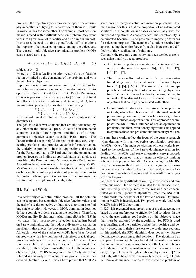
values: 3, 5, 10, 15 and 20 objectives. The parameter thatcontrols the degree of Si was defined for eleven differentvalues. The Si value varied in intervals of 0.05, the samevariation applied in [26]. Si varies in the range [0.25, 0.45],for the selection of a subset of the Pareto Front, varies in therange [0.55, 0.75] for the relaxation of the dominance rela-tion and has the value equal to 0.5 for the original Paretodominance relation.Some quality measures were used to observe how conver-gence and diversity are affected by the control of the domi-nance area of the solutions in PSO [29]. The GenerationalDistance (GD) was used to observe if the algorithm con-verges for some region of the true Pareto Front. The InverseGenerational Distance to observe if the PFapprox, i.e, thesolutions generated by the CDAS-SMPSO algorithm, con-verges to the true Pareto front and also if this set is well di-versified. The variance of the distance between neighborssolution in the front is measured by the Spacing. For thecomparison of the quality indicators the Friedman test at5% significance level is used. The Friedman test is a non-parametric statistical test used to detect differences betweenalgorithms [12]. The test is applied to raw values of eachmetric.Besides, it was performed a comparison discussed in [15] toobserve the convergence and diversity for each configuration.In literature, it is accepted that decision makers prefer solu-tions in the middle of the Pareto front, called the ”knee” ofthe Pareto front. So, in [15] it is presented a methodologythat compares the distance of each point of the PFapprox tothe knee, the Tchebycheff distance.Table 1 presents the summary of the Friedman test. For eachobjective value, the configuration with best results for eachquality measure is presented.GD best results were obtained when Si < 0.5. The configu-rations Si = 0.25, 0.3 0.35 and 0.4 obtained the best resultsfor almost all objectives, i.e., obtained a statistically signifi-cant difference with respect to other configurations. Besides,it was observed that when the number of objectives growsthe convergence of the original dominance relation deterio-rates, achieving poor GD results. For the IGD, according tothe Friedman test, the results of the configurations Si = 0.3,0.35, 0.4 and 0.45 had the best results. Again, for IGD whenthe number of objectives is small, the SMPSO with the orig-inal Pareto dominance relation still has competitive IGD re-sults; however, when this number grows its performance de-teriorates. It was concluded examining these two indicatorsthat the CDAS with Si < 0.5 produced very good results formany objectives.For the spacing indicator, the best configuration accordingto the Friedman test was the extreme Si = 0.25. However,this occurs because for almost all objective this configura-tion generated only one solution in the PFapprox. Again, theconfiguration with the original Pareto dominance relation ob-tained the worst results.For the Tchebycheff analysis, the original dominance pro-duced distributions that were not concentrated in any re-gion, generating equivalent distributions for different dis-tances. These distributions reflect the results of GD andIGD. The SMPSO with the original Pareto dominance re-lation do not converge to the true Pareto Front, but, it gener-

ates a distributed PFapprox because its IGD values are low,consequently, it generates a sub-optimal solution. The bestdistributions were the configurations Si = 0.35, 0.4 and0.45. These configurations concentrated almost all its so-lutions in a small distance of the knee, even when dealingwith high number of objectives. These concentrated distribu-tions stress the GD and IGD results and show that the CDASwith Si < 0.5 improves the convergence of the PSO algo-rithm. For low values of Si, only few solutions remain non-dominated and the algorithm converges for a small region,often close to the knee. For configurations with Si > 0.5, itwas concluded that high values of Si produces a diversifiedPFapprox. With a degree near to the original Pareto domi-nance relation, (0.5 < Si ≤ 0.65), the solutions were con-centrated in a region with small values of the Tchebycheffdistance. However, the CDAS with Si > 0.5 did not havethe same power of convergence than Si < 0.5.

V. Ranking Based PSO

In the previous work [9], the influence of the CDAStechnique into PSO algorithm was analyzed using theSMPSO [22]. This paper extends this work by analyzing thebehavior of another many-objective technique into SMPSO.The chosen method is the Average Ranking (AR) that accord-ing to [7] produced the best results among different rankingmethods. In this section, first, the main aspects of the PSOare discussed and details about SMPSO are given. Finally,the AR and its implementation into SMPSO algorithm aredescribed. Here, the implementation of AR into SMPSO iscalled AR-SMPSO.

A. SMPSO

Particle Swarm Optimization is a population-based heuristicinspired by bird. PSO performs a cooperative search proce-dure between the solutions. The set of possible solutions isa set of particles, called swarm, which moves in the searchspace through the velocity operator that is based on the bestpositions of their neighbors (social component), the leader,and on their own best position (local component).Multi-objective particle swarm optimization uses Paretodominance concepts to define the leaders. Each particle ofthe swarm could have different leaders, but only one may beselected to update the velocity. The basic steps of a MOPSOalgorithm are: initialization of the particles, computation ofthe velocity, position update, mutation and update of leader’sarchive.Each particle pi, at a time step t, has a position x(t) ∈Rn (3), that represents a possible solution. The position ofthe particle, at time t + 1, is obtained by adding its velocity,v(t) ∈ Rn (4), to x(t):

−→x (t+ 1) = −→x (t) +−→v (t+ 1) (3)

The velocity of a particle pi is based on the best position al-ready fetched by the particle, −→p best(t), and the best positionalready fetched by the set of neighbors of pi,

−→Rh(t), that is a

leader from the repository. The velocity is defined as follows:

−→v (t+ 1) = $ · −→v (t) + (C1 · φ1) · (−→p best(t)−−→x (t))

+(C2 · φ2) · (−→Rh(t)−−→x (t)) (4)

Carvalho and Pozo099

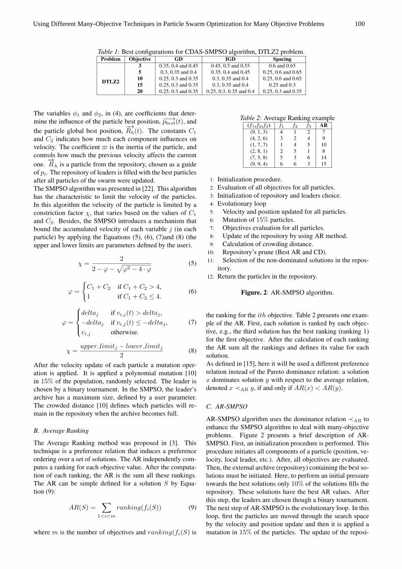
Table 1: Best configurations for CDAS-SMPSO algorithm, DTLZ2 problem.Problem Objective GD IGD Spacing

DTLZ2

3 0.35, 0.4 and 0.45 0.45, 0.5 and 0.55 0.6 and 0.655 0.3, 0.35 and 0.4 0.35, 0.4 and 0.45 0.25, 0.6 and 0.6510 0.25, 0.3 and 0.35 0.3, 0.35 and 0.4 0.25, 0.6 and 0.6515 0.25, 0.3 and 0.35 0.3, 0.35 and 0.4 0.25 and 0.320 0.25, 0.3 and 0.35 0.25, 0.3, 0.35 and 0.4 0.25, 0.3 and 0.35

The variables φ1 and φ2, in (4), are coefficients that deter-mine the influence of the particle best position, −−→pbest(t), andthe particle global best position,

−→Rh(t). The constants C1

and C2 indicates how much each component influences onvelocity. The coefficient $ is the inertia of the particle, andcontrols how much the previous velocity affects the currentone.

−→Rh is a particle from the repository, chosen as a guide

of pi. The repository of leaders is filled with the best particlesafter all particles of the swarm were updated.The SMPSO algorithm was presented in [22]. This algorithmhas the characteristic to limit the velocity of the particles.In this algorithm the velocity of the particle is limited by aconstriction factor χ, that varies based on the values of C1

and C2. Besides, the SMPSO introduces a mechanism thatbound the accumulated velocity of each variable j (in eachparticle) by applying the Equations (5), (6), (7)and (8) (theupper and lower limits are parameters defined by the user).

χ =2

2− ϕ−√ϕ2 − 4 · ϕ

(5)

ϕ =

C1 + C2 if C1 + C2 > 4,1 if C1 + C2 ≤ 4.

(6)

ϕ =

deltaj if vi,j(t) > deltaj ,−deltaj if vi,j(t) ≤ −deltaj ,vi,j otherwise.

(7)

χ =upper limitj − lower limitj

2(8)

After the velocity update of each particle a mutation oper-ation is applied. It is applied a polynomial mutation [10]in 15% of the population, randomly selected. The leader ischosen by a binary tournament. In the SMPSO, the leader’sarchive has a maximum size, defined by a user parameter.The crowded distance [10] defines which particles will re-main in the repository when the archive becomes full.

B. Average Ranking

The Average Ranking method was proposed in [3]. Thistechnique is a preference relation that induces a preferenceordering over a set of solutions. The AR independently com-putes a ranking for each objective value. After the computa-tion of each ranking, the AR is the sum all these rankings.The AR can be simple defined for a solution S by Equa-tion (9):

AR(S) =∑

1<i<m

ranking(fi(S)) (9)

where m is the number of objectives and ranking(fi(S) is

Table 2: Average Ranking example(f1,f2,f3) f1 f2 f3 AR

(9, 1, 3) 4 1 2 7(4, 2, 6) 3 2 4 9(1, 7, 7) 1 4 5 10(2, 8, 1) 2 5 1 8(7, 5, 8) 5 3 6 14(9, 9, 4) 6 6 3 15

1: Initialization procedure.2: Evaluation of all objectives for all particles.3: Initialization of repository and leaders choice.4: Evolutionary loop5: Velocity and position updated for all particles.6: Mutation of 15% particles.7: Objectives evaluation for all particles.8: Update of the repository by using AR method.9: Calculation of crowding distance.

10: Repository’s prune (Best AR and CD).11: Selection of the non-dominated solutions in the repos-

itory.12: Return the particles in the repository.

Figure. 2: AR-SMPSO algorithm.

the ranking for the ith objective. Table 2 presents one exam-ple of the AR. First, each solution is ranked by each objec-tive, e.g., the third solution has the best ranking (ranking 1)for the first objective. After the calculation of each rankingthe AR sum all the rankings and defines its value for eachsolution.As defined in [15], here it will be used a different preferencerelation instead of the Pareto dominance relation: a solutionx dominates solution y with respect to the average relation,denoted x ≺AR y, if and only if AR(x) < AR(y).

C. AR-SMPSO

AR-SMPSO algorithm uses the dominance relation ≺AR toenhance the SMPSO algorithm to deal with many-objectiveproblems. Figure 2 presents a brief description of AR-SMPSO. First, an initialization procedure is performed. Thisprocedure initiates all components of a particle (position, ve-locity, local leader, etc.). After, all objectives are evaluated.Then, the external archive (repository) containing the best so-lutions must be initiated. Here, to perform an initial pressuretowards the best solutions only 10% of the solutions fills therepository. These solutions have the best AR values. Afterthis step, the leaders are chosen though a binary tournament.The next step of AR-SMPSO is the evolutionary loop. In thisloop, first the particles are moved through the search spaceby the velocity and position update and then it is applied amutation in 15% of the particles. The update of the reposi-

100Using Different Many-Objective Techniques in Particle Swarm Optimization for Many Objective Problems

tory is the main difference from AR-SMPSO to the originalSMPSO. In this step, the the ≺AR relation is applied. Onesolution enters in the repository if and only if it dominatesany other solution with respect to the average relation. Then,the Crowded Distance (CD) is calculated for all solutions inthe repository. As presented in Section V-A, the SMPSOalgorithm limits the number of solutions in the repository.So, it must occur a prune procedure. This prune procedurekeeps the solutions with best AR. If the AR is equal, thenCD is used. Finally, to perform a pressure towards the Paretofront, only the nondominated solutions are kept in the exter-nal archive.Next Section presents the empirical experiments performedto evaluate the AR-SMPSO algorithm. It is analyzed howthe AR influences convergence and diversity of the SMPSO’ssearch for many objectives problems. Besides, its results arecompared to SMPSO and CDAS-SMPSO algorithms.

VI. Experiments

In this section, it is presented an empirical analysis to in-vestigate the performance of PSO with many-objective tech-niques for many objective problems. Here, the two many-objective techniques discussed before are used: control ofdominance area of solutions, called CDAS-SMPSO, and theAverage Ranking, called AR-SMPSO.The modified algorithms were applied to 2 many-objectiveproblems of the DTLZ family [11], DTLZ2 and DTLZ4.The DTLZ family are a set of benchmark problems oftenused in the analysis of MOEAs [22] [27]. These problemswere selected for this study because they share the followingimportant features: a) the relatively small implementationeffort(Bottom-up approach and constraint surface approach),b) can be scaled to any number of objectives (M) and deci-sion variables (n), c) the global Pareto front is known analyt-ically, d) convergence and diversity difficulties can be easilycontrolled. For each problem, the variable k represents thecomplexity of the search, where k = n - M + 1 (n number ofvariables, M number of objectives). The problems are builtwith non-overlapping sets of decision variables and |xM | =k. The DTLZ2 problem can be used to investigate the abilityof the algorithms to scale up its performance in large numberof objectives. The DTLZ4 problem is used in order to inves-tigate the ability to maintain a good distribution of solutions.In this study, we are interested to analyze the behavior ofthe modified PSO algorithms with the many-objectives tech-niques for many objectives. So, in the empirical study, thealgorithms are applied to different problems and high dimen-sional objective spaces: 3, 5, 10, 15 and 20.The same way as presented in the previous work [9], here,this experimental study had the goal to investigate the behav-ior of the proposed approaches, especially in terms of conver-gence and diversity, as well as their scalability with respect tothe number of objectives functions. So, the this set of qualitymeasures is used:Generational Distance (GD) measures how far the gener-ated approximated Pareto front PFapprox, i.e, the solutionsgenerated by the algorithms, are from the true Pareto frontof the problem PFtrue. If GD is equal to 0 all points ofPFapprox belong to the true Pareto front. GD allows observ-ing if the algorithm converges for some region of the true

Pareto Front.Inverse Generational Distance (IGD) measures the mini-mum distance of each point of the PFtrue to the points ofthe PFapprox. If IGD is equal to zero, the PFapprox containsevery point of the true Pareto Front. IGD allows to observeif the PFapprox converges to the true Pareto front and also ifthis set is well diversified. It is important to perform a jointanalysis of the GD and IGD indicators because if only GDis considered it is not possible to identify if the solutions aredistributed over the entire Pareto front. On the other hand, ifonly IGD is considered it is possible to define a sub-optimalsolution as a good solution.Spacing [29] measures the range variance between neigh-bors solution in the front. If the value of this metric is 0, allsolutions are equally distributed in the objective space.We also compared the Execution Time of each algorithmand performed an analysis of the distribution of the Tcheby-cheff distance:The distribution of the Tchebycheff distance is a metricdefined on a vector space where the distance between twovectors is the greatest of their differences along any coordi-nate dimension, Equation (10). Here, this distance is usedto measures the minimum Tchebycheff distance of each ap-proximation obtained to the ideal point, z., or the ”knee” ofthe Pareto front. The distributions of the Tchebycheff dis-tance for all solutions are presented in distribution graphs, forall analyzed objectives. The main motivation to use this met-ric is because in literature, it is accepted that decision makersprefer solutions in the middle of the Pareto front, called the”knee” of the Pareto front [8].

d(z, z∗, λ) = max1≤j≤mλj |z∗j − zj | (10)

z∗ is the knee of the Pareto front, z is an objective vector inPFapprox, m is the number of objectives and λj = 1/Ri,where Ri is the range of the j − th objective in the truePareto Front.

For the CDAS-SMPSO, the parameter that controls de degreeof Si is defined for eleven different values, performing differ-ent configurations. The Si value varied in intervals of 0.05,the same variation applied in [26]. Si varies in the range[0.25, 0.45], for the selection of a subset of the Pareto Front,varies in the range [0.55, 0.75] for the relaxation of the dom-inance relation and has the value equal to 0.5 for the originalPareto dominance relation. The AR-SMPSO, did not needany specific parameter configuration.Both algorithms were executed fifty times. All configura-tions, each Si value and AR, were executed with 100 gener-ations and 250 particles. ω varies in the interval [0, 0.8], andboth φ1 and φ2 vary in the range [0, 1]. C1 and C2 vary inthe interval [1.5, 2.5]. The size of the repository is defined asthe same size of the population. It is applied a polynomialmutation with probability pm = 1/n, where n is the numberof variables of the problem. Each variable of the velocity islimited to the range [−5,+5]. All parameters were definedwith the values presented in [22].Next Section describes the results of this empirical study.First, similar experiments to [9] are presented, only using theCDAS-SMPSO, but now using the DTLZ4 problem. Theseexperiments compare each configuration of CDAS and ana-

Carvalho and Pozo101

lyze all quality indicators and then, the best configurationsfor each indicator are selected.After, the results of AR-SMPSO were compared to each bestconfiguration of CDAS-SMPSO and to the original domi-nance relation, Si = 0.5, for all quality indicator. Also, thedistribution of the Tchebycheff is discussed.

A. Results

Table 3 presents the best configurations obtained for theDTLZ4 problem, for each indicator. For GD, the configu-rations Si < 0.5 exhibited best results. In this problem, onlySi < 0.5 had the best results, especially Si = 0.35, 0.4 and0.45. For IGD, the CDAS-SMPSO obtained similar resultsto DTLZ2 problem. Good results for Si < 0.5, especiallySi = 0.25, 0.45 and 0.55. These results stress that using lowvalues of Si we can have good convergence and diversity inmost cases, but there are some situations that the opposite canbe true. For Spacing, it can be highlighted that good spacingresults were obtained with low values of Si. This often oc-curs due to the small number of solutions. The best spacingresults were obtained with the configurations that generatedsmaller set of solutions.Tables 4, 5, 6 and 7 present the results of the comparison be-tween CDAS-SMPSO and AR-SMPSO. Each table presentsthe mean value of the indicators, for all executions. The cellsmarked with ∗ represent configurations that did not partici-pate in the comparison, only best configurations of CDAS-SMPSO were selected.For GD, Table 4, the CDAS-SMPSO outperformed the AR-SMPSO for all number of objectives, for both problems. Itcan be observed that when the number of objective growsthe difference between the techniques decreases. Besides,the AR-SMPSO obtained best results than the original dom-inance relation for all comparisons. In sum, the CDAS tech-nique obtained the best convergence, however AR-SMPSOalso obtained good convergence and did not deteriorate whenthe number of objective grows.Table 5 presents the IGD results. Again, the best results wereobtained by the CDAS technique. For the DTLZ2 problem,the CDAS-SMPSO obtained the best results for all numberof objectives, however the AR-SMPSO obtained very closeresults. The AR technique obtained better IGD than usingthe original dominance relation and its results did no deteri-orate for high number of objectives. For DTLZ4, the CDAS-SMPSO obtained much better IGD than the others. As for theGD, the difference between AR-SMPSO and CDAS-SMPSOdecreases when the number of objective grows. Again,AR-SMPSO outperformed the original dominance relation.Therefore, it can be concluded that CDAS-SMPSO gener-ated a more distributed PFapprox than AR-SMPSO and bothalgorithms performed better than the original dominance re-lation considering convergence and distribution.The results were similar for the Spacing indicator, presentedat Table 6. CDAS-SMPSO obtained the best results, for bothproblems. This occurs due to the small number of solutionsgenerated by this algorithm. As discussed in [9], the smallerthe size of PFapprox is, the smaller is the spacing. The AR-SMPSO generated a constant number of solutions, often asbig as the size of the repository. Again, the AR-SMPSO ob-tained better results than the original dominance relation.

Table 7 presents the average execution time, in seconds,for all CDAS-SMPSO configurations and AR-SMPSO. ForDTLZ2, the CDAS-SMPSO obtained the best executiontime, but only for the configuration with Si = 0.25. Thisconfiguration obtained a low execution time due to the smallPFapprox. The AR-SMPSO executed much faster than theothers configurations, including the original dominance re-lation. For the DTLZ4, the results were different. TheCDAS-SMPSO executed faster than the AR-SMPSO, espe-cially when Si < 0.5. This occurred because the CDAS-SMPSO generated a smaller PFapprox, for all objective stud-ied. It is important to highlight, that this small set of solutionsdid not deteriorate the quality of the algorithms.In summary, the CDAS technique was the best many-objective technique. It outperformed the AR for all indica-tors analyzed. The CDAS-SMPSO obtained better conver-gence and diversity than AR-SMPSO. However, AR-SMPSOobtained better results than the original dominance relation,especially when the number of objective grows. Also, AR-SMPSO does not require an extra parameter and this is animportant advantage. It also executes faster, independentlyof the problem. For the CDAS-SMPSO, the user parameterSi influences the quality of the search. This algorithm ob-tained best results with different values of Si, however, it canbe stated that Si lower than 0.5 generates the best results. Itwas also showed that, the CDAS-SMPSO can execute faster,however this execution time is directly related to the numberof solutions and there is no guaranteed that this algorithmwill be faster for every problem.

B. Tchebycheff distribution analysis

Figures 3 and 4 present the distribution of the Tcheby-cheff distance for best configurations of CDAS-SMPSO, AR-SMPSO and SMPSO( Si = 0.5), for all number of objec-tives. Here, algorithms that have more solutions around theknee are better, i.e, the algorithm that concentrates its distri-bution in a smaller Tchebycheff distance.For the DTLZ2 problem, the CDAS-SMPSO produced thebest distribution. For 3 and 5 objectives, all configurationsgenerated its distributions concentrated in low Tchebycheffvalues, i.e., near the knee. When the number of objectivesgrows, only the configurations Si = 0.25 and 0.3 still con-centrated its distributions near the knee. The other ones, pro-duced a more diversified distribution. As presented in [9],the original dominance relation, Si = 0.5, produced a sim-ilar distribution for almost all objectives, for both problems.The solutions of these configurations are distributed throughdifferent distances. Furthermore, these distributions were farfrom the knee. This same diversification of the distributionsoccurred for the AR-SMPSO.For DTLZ4, similar results can be observed. Again, the orig-inal dominance relation and AR-SMPSO generated diversi-fied distributions. However, AR-SMPSO concentrated its so-lutions farther from the knee than the original dominancerelation. Again the best results were obtained by CDAS-SMPSO. For this problem, almost all generated solutionswere concentrated at the same Tchebycheff distance, closerto the knee.In sum, the CDAS-SMPSO was the best technique, now con-sidering the distance from the knee. It generated almost all

102Using Different Many-Objective Techniques in Particle Swarm Optimization for Many Objective Problems

Table 3: Best configurations for CDAS-SMPSO algorithm, for DTLZ4 problem.

Problem Objective GD IGD Spacing

DTLZ4

3 0.25, 0.3 0.35, 0.4 and 0.45 0.25, 0.3 and 0.7 0.25 and 0.755 0.35, 0.4 and 0.45 0.25, 0.3 and 0.35 0.25 and 0.75

10 0.35, 0.4 and 0.45 0.25, 0.3 and 0.35 0.25, 0.3 and 0.3515 0.35, 0.4 and 0.45 0.25, 0.3 and 0.35 0.25, 0.3 and 0.3520 0.35, 0.4 and 0.45 0.25, 0.3, 0.35 and 0.4 0.25, 0.3 and 0.35

Table 4: GD values for best CDAS-SMPSO configurations, original dominance and AR-SMPSO, for each number of objec-tives and for both DTLZ problems.

Prob Obj 0.25 0.3 0.35 0.4 0.45 0.5 0.55 0.6 0.65 0.7 0.75 AR

DTLZ2

3 * * 3.17E-03 2.45E-03 3.64E-03 1.59E-02 * * * * * 1.52E-025 * 1.23E-02 9.85E-03 1.37E-02 * 6.42E-02 * * * * * 4.47E-02

10 1.94E-02 2.48E-02 3.73E-02 * * 1.32E-01 * * * * * 6.22E-0215 2.24E-02 2.67E-02 5.04E-02 * * 1.60E-01 * * * * * 8.68E-0220 1.85E-02 2.82E-02 5.32E-02 * * 1.75E-01 * * * * * 1.11E-01

DTLZ4

3 5.25E-05 6.01E-05 5.81E-05 6.48E-05 8.02E-05 9.60E-03 * * * * * 1,52E-025 * 1.23E-02 9.85E-03 1.37E-02 * 6.42E-02 * * * * * 3.97E-02

10 1.94E-02 2.48E-02 3.73E-02 * * 1.32E-01 * * * * * 6.22E-0215 2.24E-02 2.67E-02 5.04E-02 * * 1.60E-01 * * * * * 8.68E-0220 1.85E-02 2.82E-02 5.32E-02 * * 1.75E-01 * * * * * 1.09E-01

Table 5: IGD values for best CDAS-SMPSO configurations, original dominance and AR-SMPSO, for each number of objec-tives and for both DTLZ problems.

Prob Obj 0.25 0.3 0.35 0.4 0.45 0.5 0.55 0.6 0.65 0.7 0.75 AR

DTLZ2

3 * * * * 7.77E-04 9.46E-04 8.78E-04 * * * * 1.84E-035 * * 2.85E-03 2.32E-03 2.47E-03 4.93E-03 * * * * * 4.56E-0310 * 3.61E-03 3.24E-03 3.69E-03 * 1.10E-02 * * * * * 5.54E-0315 * 3.24E-03 3.43E-03 4.12E-03 * 1.45E-02 * * * * * 5.77E-0320 4.84E-03 3.61E-03 3.24E-03 3.69E-03 * 1.10E-02 * * * * * 6.20E-03

DTLZ4

3 5.31E-03 7.06E-03 * * * 2.91E-02 * * * 1.15E-02 * 2.74E-035 3.10E-04 3.87E-04 4.82E-04 * * 1.37E+00 * * * * * 1.46E-0310 1.63E-06 2.36E-06 3.11E-06 * * 2.04E+00 * * * * * 1.20E-0315 4.44E-08 8.21E-08 9.27E-08 * * 2.18E+00 * * * * * 1.68E-0320 4.04E-09 7.56E-09 9.94E-09 1.44E-08 * 2.23E+00 * * * * * 1.87E-04

Table 6: Spacing values for best CDAS-SMPSO configurations, original dominance and AR-SMPSO, for each number ofobjectives and for both DTLZ problems.

Prob Obj 0.25 0.3 0.35 0.4 0.45 0.5 0.55 0.6 0.65 0.7 0.75 AR

DTLZ2

3 * * * * * 8.08E-01 * 4.11E-01 2.11E-01 * * 8.79E-015 4.46E-01 * * * * 1.53E+00 * 6.82E-01 1.51E-01 * * 1.27E+0010 * 4.96E-01 2.39E+00 1.27E+00 * 8.78E-01 * * * * * 1.36E+0015 5.53E-01 7.57E-01 * * * 2.54E+00 * * * * * 1.82E+0020 5.52E-01 7.47E-01 9.84E-01 * * 2.56E+00 * * * * * 2.28E+00

DTLZ4

3 5.31E-03 * * * * 5.10E-01 * * * * 8.76E-02 3.55E-015 3.10E-04 * * * * 1.37E+00 * * * * 1.35E-01 5.73E-0110 1.63E-06 2.36E-06 3.11E-06 * * 2.04E+00 * * * * * 8.50E-0115 4.44E-08 8.21E-08 9.27E-08 * * 2.18E+00 * * * * * 8.31E-0120 4.04E-09 7.56E-09 9.94E-09 * * 2.23E+00 * * * * * 7.73E-01

Table 7: Execution time (seconds) for all configurations of CDAS-SMPSO and AR-SMPSO, for each number of objectivesand for both DTLZ problems.

Prob Obj 0.25 0.3 0.35 0.4 0.45 0.5 0.55 0.6 0.65 0.7 0.75 AR

DTLZ2

3 0.52 1.44 6.42 34.32 39.05 32.88 43.44 43.60 42.22 35.82 61.73 4.725 1.60 33.65 66.56 475.11 160.80 68.85 589.97 184.03 23.92 97.48 614.71 8.50

10 7.37 758.33 144.74 1091.48 962.58 157.86 609.50 451.70 210.78 148.25 653.08 15.7215 12.61 626.27 446.05 1037.35 344.03 434.92 791.24 478.90 628.44 1010.35 776.83 23.4820 21.05 1078.43 602.08 979.36 865.95 1020.49 820.51 1182.44 815.63 731.59 954.37 32.77

DTLZ4

3 0.92 2.49 3.01 3.90 4.97 9.58 5.93 5.35 4.25 2.09 8.67 3.325 2.16 5.20 6.25 7.85 10.10 17.70 9.81 7.96 5.55 4.21 11.01 8.76

10 3.56 5.91 7.36 8.00 11.53 35.22 11.98 10.09 8.23 9.60 16.99 19.9515 10.73 16.18 16.89 21.09 25.25 124.62 34.04 28.52 24.65 25.27 60.65 30.2220 19.17 25.24 27.18 31.25 36.27 166.01 47.83 41.03 36.56 39.44 112.57 40.28

Carvalho and Pozo103

(a) 3 objectives (b) 5 objectives

(c) 10 objectives (d) 15 objectives

(e) 20 objectives

Figure. 3: Distribution of Tchebycheff distance for CDAS-SMPSO (best GD or IGD) and AR-SMPSO in DTLZ2 problem.

104Using Different Many-Objective Techniques in Particle Swarm Optimization for Many Objective Problems

(a) 3 objectives (b) 5 objectives

(c) 10 objectives (d) 15 objectives

(e) 20 objectives

Figure. 4: Distribution of Tchebycheff distance for CDAS-SMPSO (best GD or IGD) and AR-SMPSO in DTLZ4 problem.

Carvalho and Pozo105

its solution near the knee for both problems and for all num-ber of objectives. Examining of the quality indicators and thedistribution of Tchebycheff distance, the CDAS-SMPSO ob-tained very good results: good convergence, diversity and itssolutions were generated near the knee of the Pareto front.The AR-SMPSO produced a more diversified distribution,but far from the knee. This result was expected because, aspresented in [15] for the NSGAII algorithm, the AR tends toproduce extreme solutions of the Pareto front, not near theknee.

VII. Conclusion

This work presented a study of the influence of some many-objective techniques in particle swarm optimization, formany objective problems. Two different many-objective ap-proaches were used: Control of Dominance Area of Solutionand Average Ranking. These techniques were applied to amulti-objective PSO algorithm (SMPSO) that is based in co-operation of individuals, a few explored topics in literature.A set of empirical experiments was performed to measurehow CDAS and AR affect the convergence and diversity ofthe PSO algorithm. Besides, the algorithms were confrontedto observe which technique obtained the best results in many-objective scenarios. The CDAS-SMPSO were evaluated intwo different situations, using Si < 0.5, i.e, selecting a sub-set of the Pareto Front and using Si > 0.5, i.e, performinga relaxation of the Pareto dominance relation. Ten differ-ent SMPSO configurations were used: 5 with Si < 0.5 and5 with Si > 0.5. The original Pareto dominance relation(Si = 0.5) was also used.The experiments were conducted with two different many-objective problems, DTLZ2 and DTLZ4, and the number ofobjectives were varied in five different values: 3, 5, 10, 15and 20. Three quality indicators were used: generational dis-tance, inverse generational distance and spacing. Also, theexecution time was analyzed. Besides, the distribution of theTchebycheff distance of the generated solutions to the kneeof the true Pareto front was analyzed.First, the best CDAS-SMPSO configurations were obtainedfor both problems, for each quality indicator. After, thesebest configurations were confronted to AR-SMPSO algo-rithm and the original dominance relation. In this analysis,the best results were obtained by CDAS-SMPSO, for all in-dicators analyzed. Besides, this algorithm executed fasterthan AR-SMPSO. However, this execution time is defined bythe number of solutions, the smaller the number of solutionsthe faster is the execution time. AR-SMPSO results wereoutperformed by CDAS-SMPSO, but AR-SMPSO obtainedbetter results than the original dominance relation, especiallywhen the number of objective grows. Furthermore, the AR-SMPSO does not require any additional parameter and it ex-ecutes fast independently of the problem. Through the anal-ysis of all quality indicators and the Tchebycheff distance,it can be concluded that CDAS-SMPSO was the best tech-nique. It generates its solutions near the knee of the Paretofront, for all problems and objectives. The AR-SMPSO pro-duced a diversified distribution, often far from the knee. Thisoccurs, because the AR technique prefers extreme solutionsin the Pareto front.Future works include expanding the experiments to a higher

number of problems and objectives, to search for other many-objective techniques and to confront the results of PSO withother MOEAs.

References

[1] H. Aguirre and K. Tanaka. Adaptive e-ranking on many-objective problems. Evolutionary Intelligence, 2(4):183–206,2009.

[2] H. Aguirre and K. Tanaka. Space partitioning evolutionarymany-objective optimization: Performance analysis on mnk-landscapes. Transactions of the Japanese Society for ArtificialIntelligence, 25(2):363–376, 2010.

[3] P. J. Bentley and J. P. Wakefield. Finding acceptable solutionsin the pareto-optimal range using multiobjective genetic algo-rithms. In P. K. Chawdhry, R. Roy, and R. K. Pant, editors,Soft Computing in Engineering Design and Manufacturing,pages 231–240. Springer-Verlag, January 1998.

[4] D. Brockhoff and E. Zitzler. Are all objectives necessary? ondimensionality reduction in evolutionary multiobjective opti-mization. In T. Runarsson, H.-G. Beyer, E. Burke, J. Merelo-Guervos, L. Whitley, and X. Yao, editors, Parallel ProblemSolving from Nature - PPSN IX, volume 4193 of LectureNotes in Computer Science, pages 533–542. Springer Berlin /Heidelberg, 2006.

[5] D. Brockhoff and E. Zitzler. Objective reduction in evolu-tionary multiobjective optimization: Theory and applications.Evolutionary Computation, 17(2):135–166, 2009.

[6] C. A. C. Coello, G. B. Lamont, and D. A. V. Veldhuizen. Evo-lutionary Algorithms for Solving Multi-Objective Problems(Genetic and Evolutionary Computation). Springer-VerlagNew York, Inc., Secaucus, NJ, USA, 2006.

[7] D. W. Corne and J. D. Knowles. Techniques for highly multi-objective optimisation: some nondominated points are betterthan others. In GECCO ’07: Proceedings of the 9th annualconference on Genetic and evolutionary computation, pages773–780, New York, NY, USA, 2007. ACM.

[8] I. Das. On characterizing the knee of the pareto curve basedon normal-boundary intersection,, volume = 18, year = 1999.Structural Optimization, (2-3):107–115.

[9] A. B. de Carvalho and A. Pozo. Analyzing the control ofdominance area of solutions in particle swarm optimizationfor many-objective. In 2010 10th International Conferenceon Hybrid Intelligent Systems, pages 103–108, 2010.

[10] K. Deb, A. Pratap, S. Agarwal, and T. Meyarivan. A fastand elitist multiobjective genetic algorithm: NSGA-II. IEEETransactions on Evolutionary Computation, 6(2):182–197,August 2002.

[11] K. Deb, L. Thiele, M. Laumanns, and E. Zitzler. Scal-able multi-objective optimization test problems. In Congresson Evolutionary Computation (CEC 2002), pages 825–830,2002.

[12] J. Demsar. Statistical comparisons of classifiers over multipledata sets. The Journal of Machine Learning Research, 7:1–30, 2006.

[13] V. E. Gopal, M. V. N. K. Prasad, and V. Ravi. A fast andelitist multiobjective genetic algorithm: NSGA-II. Interna-tional Journal of Computer Information Systems and Indus-trial Management Applications (IJCISIM), 2:121–136, 2010.

[14] H. Ishibuchi, N. Tsukamoto, and Y. Nojima. Evolutionarymany-objective optimization: A short review. In CEC 2008.IEEE Congress on Evolutionary Computation, pages 2419–2426, 2008.

[15] A. L. Jaimes and C. A. C. Coello. Study of preference rela-tions in many-objective optimization. Proceedings of the 11thAnnual conference on Genetic and evolutionary computation- GECCO ’09, pages 611–618, 2009.

106Using Different Many-Objective Techniques in Particle Swarm Optimization for Many Objective Problems

[16] A. L. Jaimes, C. A. C. Coello, and D. Chakraborty. Objec-tive reduction using a feature selection technique. In GECCO’08: Proceedings of the 10th annual conference on Geneticand evolutionary computation, pages 673–680, New York,NY, USA, 2008. ACM.

[17] A. L. Jaimes, L. V. S. Quintero, and C. A. C. Coello. Rankingmethods in many-objective evolutionary algorithms. Studiesin Computational Intelligence, 193:413–434, 2009.

[18] J. Kennedy and R. Eberhart. Particle swarm optimization. InIEEE International Conference on Neural Networks, pages1942–1948. IEEE Press, 1995.

[19] I. Kokshenev and A. P. Braga. An efficient multi-objectivelearning algorithm for rbf neural network. Neurocomputing,73(16-18):2799–2808, 2010. 10th Brazilian Symposium onNeural Networks (SBRN2008).

[20] M. Koppen and K. Yoshida. Many-objective particle swarmoptimization by gradual leader selection. In ICANNGA ’07:Proceedings of the 8th international conference on Adaptiveand Natural Computing Algorithms, Part I, pages 323–331,Berlin, Heidelberg, 2007. Springer-Verlag.

[21] P. Lindroth, M. Patriksson, and A.-B. Stromberg. Approxi-mating the pareto optimal set using a reduced set of objec-tive functions. European Journal of Operational Research,207(3):1519–1534, 2010.

[22] A. Nebro, J. Durillo, J. Garcia-Nieto, C. A. C. Coello,F. Luna, and E. Alba. SMPSO: A new pso-based metaheuris-tic for multi-objective optimization. In IEEE symposiumon Computational intelligence in miulti-criteria decision-making, 2009. mcdm ’09, pages 66–73, 2009.

[23] V. Pareto. Manuel d”economie politique, 1927.[24] M. Reyes-Sierra and C. A. C. Coello. Multi-objective parti-

cle swarm optimizers: A survey of the state-of-the-art. In-ternational Journal of Computational Intelligence Research,2(3):287–308, 2006.

[25] A. H. T. K. Sato, H. Effects of moea temporally switch-ing pareto partial dominance on many-objective 0/1 knapsackproblems. Transactions of the Japanese Society for ArtificialIntelligence, 25(2):320–331, 2010. cited By (since 1996) 0.

[26] H. Sato, H. E. Aguirre, and K. Tanaka. Controlling Domi-nance Area of Solutions and Its Impact on the Performanceof MOEAs, pages 5–20. Lecture Notes in Computer Science4403: Evolutionary Multi-Criterion Optimization. Springer,Berlin, 2007.

[27] U. K. Wickramasinghe and X. Li. Using a distance metricto guide pso algorithms for many-objective optimization. InGECCO ’09: Proceedings of the 11th Annual conference onGenetic and evolutionary computation, pages 667–674, NewYork, NY, USA, 2009. ACM.

[28] Q. Zhang and H. Li. MOEA/D: A multiobjective evolutionaryalgorithm based on decomposition. IEEE Transactions onEvolutionary Computation, 11(6):712–731, 2007.

[29] E. Zitzler and L. Thiele. Multiobjective Evolutionary Algo-rithms: A Comparative Case Study and the Strength ParetoApproach. IEEE Transactions on Evolutionary Computation,3(4):257–271, 1999.

André Britto de Carvalho is a Ph.D student at the Computer Science Department on Federal University of Parana, Brazil. He received the Master degree in Computer Science at Federal University of Parana in 2009 and the BS degree in Computer Science at Federal University of Sergipe in 2006. His main interests are evolutionary algorithms metaheuristic and multiobjective

optimization. Email: andrebc@inf.ufpr.br

Aurora Trinidad Ramirez Pozo is associate professor of Computer Science Department and Numerical Methods for Engineering at Federal University of Parana,Brazil, since 1997. She received a M.S. in electrical engineering from Federal University of Santa Catarina, Brazil, in 1991. She received a Ph.D. in electrical engineering from the Federal University

of Santa Catarina, Brazil. Aurora's research interests are in evolutionary computation, data mining and complex problems.

Author Biographies

Carvalho and Pozo107