Using convolutional neural networks to predict composite properties beyond the elastic...

Artificial Intelligence Research Letter

Using convolutional neural networks to predict composite propertiesbeyond the elastic limit

Charles Yang*, Department of Mechanical Engineering, University of California, Berkeley, CA 94720, USAYoungsoo Kim*, and Seunghwa Ryu, Department of Mechanical Engineering & KI for the NanoCentury, Korea Advanced Institute of Science andTechnology, Daejeon 34141, Republic of KoreaGrace X. Gu, Department of Mechanical Engineering, University of California, Berkeley, CA 94720, USA

Address all correspondence to Seunghwa Ryu at [email protected] and Grace X. Gu at [email protected]

(Received 26 January 2019; accepted 4 April 2019)

AbstractComposites are ubiquitous throughout nature and often display both high strength and toughness, despite the use of simple base constitu-ents. In the hopes of recreating the high-performance of natural composites, numerical methods such as finite element method (FEM) areoften used to calculate the mechanical properties of composites. However, the vast design space of composites and computational cost ofnumerical methods limit the application of high-throughput computing for optimizing composite design, especially when considering theentire failure path. In this work, the authors leverage deep learning (DL) to predict material properties (stiffness, strength, and toughness)calculated by FEM, motivated by DL’s significantly faster inference speed. Results of this study demonstrate potential for DL to acceleratecomposite design optimization.

IntroductionComposite materials, which offer a variety of advantages thatcannot be gained solely with only one of their constituents,are actively used in advanced engineering applications suchas lightweight structures for aerospace and automotive indus-tries. Natural creatures also exploit composites to protect them-selves from threats in a variety of environments and to sustainliving conditions with the limited resources and building blocksavailable in nature.[1–5] Design and fabrication methods of mostman-made synthetic composites have been well establishedowing to their relatively simple arrangements. In comparison,although extensive studies have been performed to understandand mimic natural composites, it remains a daunting task to fab-ricate bio-inspired structures via conventional manufacturingprocesses because of their complex hierarchical structure rang-ing from the nano- to macro-scale. Recently, the advancementof additive manufacturing has facilitated the fabrication ofcomplex structures, and as a result, a variety of composite struc-tures inspired by natural materials such as nacre, bone,conch-shell, and spider silk have been fabricated and testedvia 3D-printing methods.[6–11]

Because many natural composites, synthesized via aself-assembly process, have relatively periodic and regulararrangements, their mechanical properties can be reasonablyunderstood by analyzing the load transfer mechanism of a

representative unit cell.[5,8,10,12] However, the applicability ofanalytical approaches is limited in accurately predicting inelas-tic responses such as fracture and plastic deformation, and pro-viding statistically meaningful results accounting for theinherent randomness in structural arrangements. Numericalmodeling based on finite element methods (FEM) can comple-ment analytical approaches for predicting properties beyond theelastic response regime such as toughness and strength e.g.,phase field simulation for the initiation and propagation of cur-vilinear cracks. Given the combinatorially large compositedesign space of even simple binary systems, it is crucial todevelop a high throughput computing procedure for the rapidin-silico testing and characterization of novel compositedesigns.[13–18] However, such numerical schemes e.g., thephase field formulation, are computationally expensive andtime consuming because they require the usage of a very finemesh to accommodate the smooth variation of the highly con-centrated stress field near the crack tip and/or damage parame-ter within the regularized diffusive width of the crack surface.The high computational cost of numerical modeling as wellas the prohibitively large design parameter space of a compos-ite makes conventional gradient-based optimization methodsthat are based on multiple/iterative evaluations of target proper-ties infeasible.

In 2012, deep learning (DL) burst onto the field of computervision, achieving record-breaking performance on theImageNet dataset, a diverse labeled image corpus with 1000different image classes.[19] Since then, DL has been used to* These authors contributed equally to this work.

MRS Communications (2019), 9, 609–617© Materials Research Society, 2019doi:10.1557/mrc.2019.49

MRS COMMUNICATIONS • VOLUME 9 • ISSUE 2 • www.mrs.org/mrc ▪ 609https://doi.org/10.1557/mrc.2019.49Downloaded from https://www.cambridge.org/core. MIT Libraries, on 16 Jul 2019 at 05:14:17, subject to the Cambridge Core terms of use, available at https://www.cambridge.org/core/terms.

mailto:[email protected]

mailto:[email protected]

https://doi.org/10.1557/mrc.2019.49

https://www.cambridge.org/core

https://www.cambridge.org/core/terms

great effect in natural language processing, reinforcementlearning, and image classification.[20] DL, which utilizes suc-cessive layers of weighted units with non-linear activations,is capable of approximating complex functions, learning to rep-resent abstract features, and using raw data as input. In additionto demonstrating excellent performance on traditional artificialintelligence (AI) benchmarks, DL has also accelerated scien-tific understanding. Neural networks have been used to predictprotein folding,[21] automatically focus a microscope for long-time periods under dynamic biologic situations,[22] speed upparticle physics simulations,[23] and optimize kirigami cuts ingraphene.[24] One common theme is that neural networks arecapable of significantly speeding up, and oftentimes improvingupon, common analytical formulas that were painstakinglycrafted by experts in the field, simply by training on largeamounts of data.

In our previous work, we demonstrated the ability of convo-lutional neural networks (CNNs), a type of neural networkarchitecture designed for computer vision tasks, to rapidlyand accurately predict material properties of composite designsas calculated by FEM, enabling high-throughput materialdesign optimization.[25,26] Previously, FEM data were calcu-lated up to the initiation of crack propagation in order to gener-ate large amounts of data quickly. In this paper, our analysiswill consider the entire crack propagation process, rather thanjust crack initiation. As a result, this problem is much morecomputationally expensive because the number of iterationsin the simulation has increased dramatically. In this work, weexplore the feasibility of using DL algorithms to predict theproperties of composites when considering the entire failurepath. The data preparation and finite element procedure usedto obtain training data for our models are discussed in the“Materials and methods” section. In the “Results and discus-sion” section, we demonstrate how CNNs outperform tradi-tional machine learning (ML) algorithms such as randomforest (RF) ensembles and linear regression. The scaling ofCNN performance with respect to the dataset size comparedwith traditional ML methods is investigated and the flexibilityof CNN architecture is utilized to improve its performance onsmaller dataset sizes. The CNNs learned convolution filtersare visualized to better understand the features the CNN islearning and to demonstrate its ability to hierarchically craftrepresentative features. Finally, we conclude and discuss futureopportunities in this research area.

Materials and methodsThis section discusses the implementation of the FEM used toobtain training data for our ML models. The data preparation,training procedures, and implementation of various algorithms,as well as the visualization algorithm for CNNs are described.

Finite element methodFEM was used to obtain our training data, with the ML algo-rithms treating the material descriptors produced by an FEMas the ground truth labels. The crack phase field solver was

based on the hybrid formulation for the quasi-static fractureof elastic solids in the commercial finite element softwareABAQUS with user-element subroutine (UEL). Our previousstudy showed that the hybrid formation adequately modelscrack propagation under combined tensile and shear loadingand crack propagation within composite materials made oftwo constituents whereas the widely used anisotropic formula-tion produces unphysical results. The details of the implemen-tation and validation can be found in our previous study.[13]

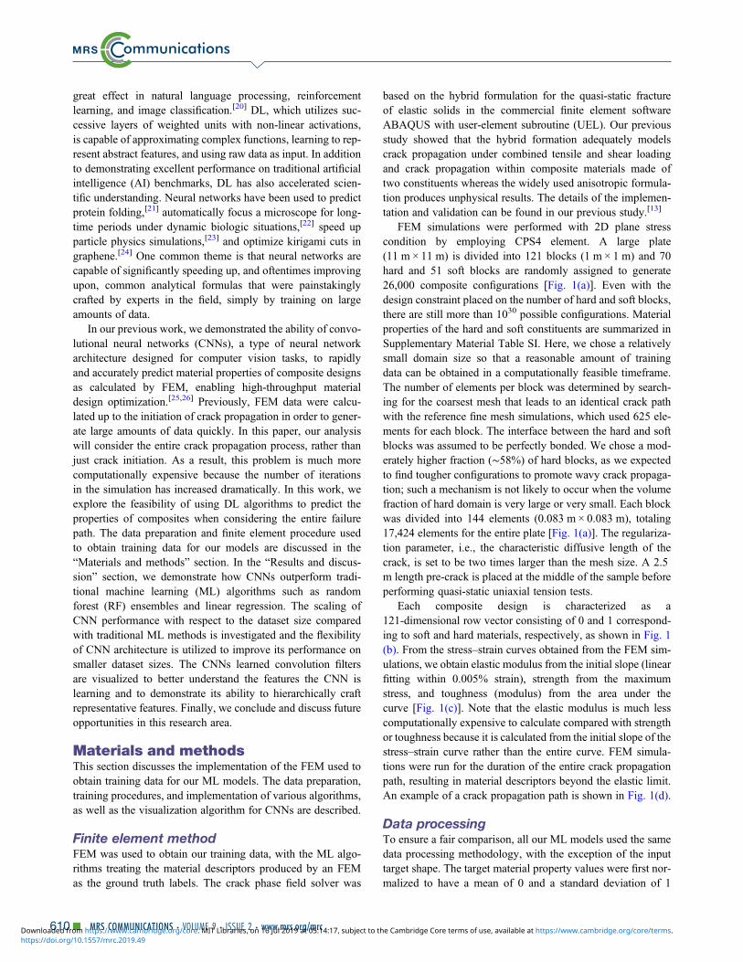
FEM simulations were performed with 2D plane stresscondition by employing CPS4 element. A large plate(11 m × 11 m) is divided into 121 blocks (1 m × 1 m) and 70hard and 51 soft blocks are randomly assigned to generate26,000 composite configurations [Fig. 1(a)]. Even with thedesign constraint placed on the number of hard and soft blocks,there are still more than 1030 possible configurations. Materialproperties of the hard and soft constituents are summarized inSupplementary Material Table SI. Here, we chose a relativelysmall domain size so that a reasonable amount of trainingdata can be obtained in a computationally feasible timeframe.The number of elements per block was determined by search-ing for the coarsest mesh that leads to an identical crack pathwith the reference fine mesh simulations, which used 625 ele-ments for each block. The interface between the hard and softblocks was assumed to be perfectly bonded. We chose a mod-erately higher fraction (∼58%) of hard blocks, as we expectedto find tougher configurations to promote wavy crack propaga-tion; such a mechanism is not likely to occur when the volumefraction of hard domain is very large or very small. Each blockwas divided into 144 elements (0.083 m × 0.083 m), totaling17,424 elements for the entire plate [Fig. 1(a)]. The regulariza-tion parameter, i.e., the characteristic diffusive length of thecrack, is set to be two times larger than the mesh size. A 2.5m length pre-crack is placed at the middle of the sample beforeperforming quasi-static uniaxial tension tests.

Each composite design is characterized as a121-dimensional row vector consisting of 0 and 1 correspond-ing to soft and hard materials, respectively, as shown in Fig. 1(b). From the stress–strain curves obtained from the FEM sim-ulations, we obtain elastic modulus from the initial slope (linearfitting within 0.005% strain), strength from the maximumstress, and toughness (modulus) from the area under thecurve [Fig. 1(c)]. Note that the elastic modulus is much lesscomputationally expensive to calculate compared with strengthor toughness because it is calculated from the initial slope of thestress–strain curve rather than the entire curve. FEM simula-tions were run for the duration of the entire crack propagationpath, resulting in material descriptors beyond the elastic limit.An example of a crack propagation path is shown in Fig. 1(d).

Data processingTo ensure a fair comparison, all our ML models used the samedata processing methodology, with the exception of the inputtarget shape. The target material property values were first nor-malized to have a mean of 0 and a standard deviation of 1

610▪ MRS COMMUNICATIONS • VOLUME 9 • ISSUE 2 • www.mrs.org/mrchttps://doi.org/10.1557/mrc.2019.49Downloaded from https://www.cambridge.org/core. MIT Libraries, on 16 Jul 2019 at 05:14:17, subject to the Cambridge Core terms of use, available at https://www.cambridge.org/core/terms.




before being passed to a ML model. All experiments were per-formed with a randomized 80/20 train/test distribution and eachexperiment used 15 trials unless otherwise stated. Each trial hada different random train/test distribution to test the model’s gen-eralizability across the entire dataset. The number of trials waslimited by the computational cost of running many trials for allmodels and material properties.

Baseline modelsMore conventional ML algorithms were used to establish abenchmark to compare DL methods with. Ordinary leastsquares (OLS) linear regression and an RF ensemble[27] with100 decision trees were used as baseline models and imple-mented using the open-source Python package scikit-learn.[28]

Default hyperparameters were used for linear regression andRF. The input was an unraveled 121-dimensional row vectorrepresenting the unit cell.

Convolutional neural networksOur CNN was implemented using the open-source pythonpackage Keras[29] with a TensorFlow backend. The batch size

for all experiments was set to 128 and the number of epochsto 100. Mean squared error (MSE) was the loss function andthe Adam optimizer was used.[30] See SupplementaryMaterial Fig. S1(a) for a full description of the model architec-ture. For CNN, an 11 × 11 matrix of binary labels is used ratherthan the 121-dimensional vector to represent the unit cell inorder to take advantage of CNNs’ ability to parameterize 2Dinputs efficiently.

CNN filter visualizationFinally, we sought to understand what kind of features the con-volution filters in each layer were learning to represent.Drawing from previous work,[31] this question can be posedas an optimization problem to maximize a given filter activationwith a matrix of constant norm. Although this is a non-convexproblem, gradient ascent can be used to find some localminima. Nesterov accelerated gradient was used as the gradientoptimizer[32] with a step size (α) of 10−5 and a momentum (γ)of 0.9 and an input image of size of 22 × 22. Although ourinputs are binary, we treat this as a continuous problem as asimplification. Intermediate values would correspond to a linear

Figure 1. (a) Mesh size description and conditions for testing and developing the composites in this paper. (b) Converting the composite material unit cellgeometry to a row vector. (c) Deriving composite material properties from the FEM simulation stress–strain curves. (d) Full crack path of composites. The crackpath is represented by removing elements whose phase is greater than 0.9. Deformation is scaled by 50.






interpolation between the soft and hard blocks. The larger inputimage size was chosen for ease of visual understanding, as thedeeper filters had more complex activations that were more eas-ily understood with larger input images. To improve our gradi-ent ascent performance, 4000 random matrices are initialized,and gradient ascent searched through the input space in parallel.Early stopping is used to prevent gradient ascent from escapinglocal minima by stopping gradient ascent after the averagescore of the best-scoring 40 inputs begins to decrease. Thebase CNN was slightly modified to have an additional convo-lution layer to better understand the effect of multiple convolu-tion layers. Although such a methodology for examining CNNfilters has been proposed previously, we expect different resultsgiven our novel, material property prediction regression task, asopposed to traditional image classification problems.

Results and discussionHere, the data used to train our model and the performance ofvarious ML models are presented. Model performance is quan-tified with a variety of metrics: MSE, mean absolute error(MAE), and the square of the Pearson correlation coefficient(R2). OLS, RF, and CNN performance with respect to datasetsize is characterized with the given metrics. Modulus as anadditional input to CNNs offers further improvements tomodel performance in smaller data regimes and visualizationsof the learned convolution filters were used to explore what fea-tures are relevant to CNNs.

Training data distributionUnderstanding the distribution of our training data is an impor-tant component of exploratory data analysis. Figures 2(a)–2(c)present the histograms of the elastic modulus, strength, andtoughness from the stress–strain curves of 26,000 configura-tions. The distribution of modulus, strength, and toughness isroughly normal with a slight right skew. Ultimately, our goalis to rapidly identify composite design patterns that exhibitproperties in the far-right tail of the distributions, oftentimesmaximizing their joint distributions e.g., high strength andtoughness. In addition, scatter plots between each pair of theset of material descriptors (elastic modulus, strength, andtoughness) show the positive correlation among all three prop-erties [Figs. 2(d)–2(f)]. This suggests that the “easy-to-obtain”elastic property (elastic modulus) may serve as a useful descrip-tor to predict “hard-to-obtain” properties (strength and tough-ness) in ML.

Comparing CNNs with benchmark modelsTo establish the relative performance of CNNs to traditionalML models, CNNs are compared with linear regression andRFs on a variety of metrics. The distribution of predicted mate-rial descriptors against their value ranking is shown in Fig. 3.For elastic modulus and strength, the CNN closely capturesthe underlying distribution, while linear regression and RFare approximating the average value of the distribution. For

toughness, RF is slightly more accurate; see Fig. S2 formodel performance as measured by MSE, MAE, and R2.

Different black-box methods can be used as a method toprobe the underlying nature of the computation required to cal-culate such values. For instance, it may be that RF performsbetter on toughness because the nested if-statements are a closerapproximation to the actual toughness calculation method. Thisoffers the intriguing possibility of creating simple analyticalmodels inspired by or derived from the trained RF model andis a research direction we plan to investigate in future work.In particular, feature importance analysis is a promising methodto “open up the black box” of ML and confirm that the algo-rithm is learning a realistic predictive model. Being able torelate the performance of different types of models to the under-lying analytical calculation would be a significant step forwardin improving and interpreting empirical models.

The design space for CNN is also very large; using tech-niques such as neural architecture search[33] to find more opti-mized architectures may improve performance of CNN beyondthat of RF. Differences in the CNN architecture for calculatingdifferent material descriptors could be hypothesized based onthe known differences in actually simulating these descriptorsor conversely, could help us further understand how to speedup simulations by using different approximation models.Finally, CNNs generally scale better with increasing data;with more data, CNNs will most likely come to outperformRF at even calculating toughness. For the rest of the paper,we will consider only CNNs, given their currently untappedpotential and excellent general performance.

Effect of dataset size of model performanceGiven the intense compute resources required to generate ourdataset, a natural question to ask is how much data are enoughto train a CNN. Another important question is when to use tra-ditional ML algorithms versus DL given a dataset of a certainsize. The performance of linear regression, RF, and CNNwith respect to the dataset size is evaluated on a variety of met-rics. The results are shown in Fig. 4 for predicting modulus.

The performance of linear regression with respect to thedataset size plateaus quickly, representing its limited modelcapacity and is generally characteristic of parametric models.RF and CNN exhibit continual improvements in performancewith dataset size as a result of being non-parametric models.However, CNN performance scales much better with largerdatasets, outstripping the performance of RF at larger datasetsizes. Note that CNNs’ superiority is not guaranteed over alldataset ranges. In the small data regime, RF and linear regres-sion perform better. Although for predicting modulus, thethreshold in dataset size occurs at around 5000 instances, thethreshold for other problems will vary based on the problemcomplexity. This threshold is a good benchmark to use fordeciding how much data are needed for problems of similarcomplexity and design. Changing experimental parameterssuch as the unit cell size will most likely increase this thresholdbut changing the ratio of hard and soft blocks should not





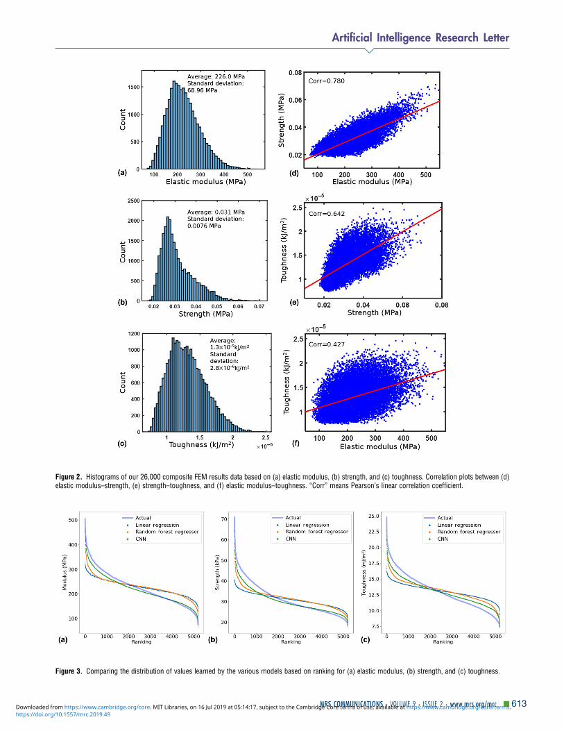
Figure 2. Histograms of our 26,000 composite FEM results data based on (a) elastic modulus, (b) strength, and (c) toughness. Correlation plots between (d)elastic modulus–strength, (e) strength–toughness, and (f) elastic modulus–toughness. “Corr” means Pearson’s linear correlation coefficient.

Figure 3. Comparing the distribution of values learned by the various models based on ranking for (a) elastic modulus, (b) strength, and (c) toughness.






significantly change this threshold. For material descriptors,some variation in the threshold results due to the differingnature of the calculations required to obtain each descriptorfrom the stress–strain curve and the metric chosen, as seen inFig. S3. The performance of linear regression, RF, and CNNwith respect to dataset size for predicting strength and tough-ness is shown in Fig. S3.

Using modulus and unit cells as CNN inputsOne potential concern with using CNN for automating FEM isthat the large initial dataset required for training may pose achallenging barrier to scalability. But, as shown in Figs. 2(d)–2(f), the existence of positive correlations between thethree material descriptors (modulus, strength, and toughness)suggests that we may be able to use the relatively lesscompute-intensive elastic modulus property as a feature tofeed into the model to improve performance on descriptorsthat are more computationally expensive to obtain with FEM.

Conveniently, neural networks are a flexible model that canefficiently parameterize and synthesize multimodal inputs e.g.,images and scalar values. Our normal CNN, which only took inthe unit cell matrix as an input, consisted of blocks of convolu-tion and max pooling layers followed by a series of dense lay-ers; batch normalization[34] and leaky ReLU activations wereused throughout. To pass in both a unit cell image and the asso-ciated modulus value, the same CNN architecture was slightlymodified by adding another smaller neural network consistingof dense and batch normalization layers, which took the mod-ulus value as input. The output of this secondary, smaller net-work was concatenated with the output of the final max poolinglayer in the CNN and fed into the series of dense and batch nor-malization layers. See Fig. S1(b) for a diagram.

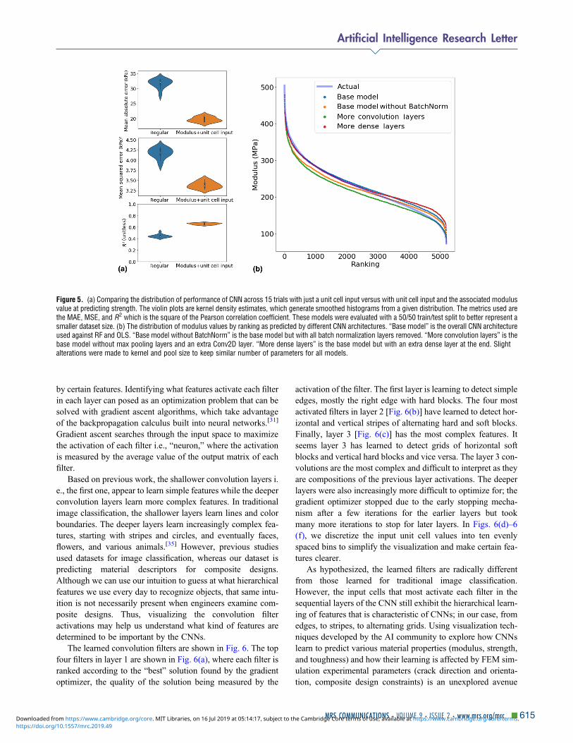
The performance of a neural network that takes in both thecomposite unit cell and the associated elastic modulus valuecompared with the regular CNN architecture that only usesthe composite unit cell at predicting strength is shown inFig. 5(a). A 50/50 train/test split was used instead of the regular80/20 train/test split to demonstrate the utility of this method in

smaller datasets. The use of modulus as an additional featureclearly improves the performance of neural networks even onsmaller datasets, demonstrating how extra information aboutcomposite properties can be leveraged in conjunction withthe flexibility of neural networks to improve inference abilities.Rather than just reporting average error values, we show thekernel density estimate of the distribution of errors, as mea-sured by a variety of metrics. The lack of overlap in violinplots in Fig. 5(a) indicates that using modulus as an additionalfeature significantly improves the performance of CNN onsmaller datasets. This augmentation technique can also beapplied to reduce the amount of training data required bymore data-intensive tasks, such as generative adversarial mod-els for solving the inverse design problem.

Testing different CNN architecturesA wide variety of hyperparameters and architecture designchoices exist when creating CNNs. To show that our resultsare generalizable for the entire family of CNN models andthat our results are not simply a result a hyperparameter tuningand behind-the-scenes CNN architecture optimization, threeother CNN models with different architectures are constructedand their performance in Fig. 5(b). Based on the rankingcurves, we can see that their performance is relatively similarand they all learn the underlying distribution of elastic modulivalues well. The generalization of CNN performance to a vari-ety of architectures signifies their potential in a variety of com-putational mechanics fields. Ranking curves for the same set ofarchitectures for predicting strength and toughness are shown inFig. S4.

Visualizing convolution filtersThe recursive convolution layers in the CNN learn to identifyfeatures that are considered important to the model over thecourse of training. Significant work has been carried out forvisualizing and understanding what types of features arelearned by convolution layers.[35] Specifically, each convolu-tion filter can be thought of as a neuron that is heavily activated

Figure 4. The effect of dataset size on the performance of various models at predicting the elastic modulus as determined by the following metrics: (a) MAE, (b)MSE, and (c) R2 which is the square of the Pearson correlation coefficient. The given dataset sizes are then fed into the models with an 80/20 train/test split. 95%confidence intervals are shown.





by certain features. Identifying what features activate each filterin each layer can posed as an optimization problem that can besolved with gradient ascent algorithms, which take advantageof the backpropagation calculus built into neural networks.[31]

Gradient ascent searches through the input space to maximizethe activation of each filter i.e., “neuron,” where the activationis measured by the average value of the output matrix of eachfilter.

Based on previous work, the shallower convolution layers i.e., the first one, appear to learn simple features while the deeperconvolution layers learn more complex features. In traditionalimage classification, the shallower layers learn lines and colorboundaries. The deeper layers learn increasingly complex fea-tures, starting with stripes and circles, and eventually faces,flowers, and various animals.[35] However, previous studiesused datasets for image classification, whereas our dataset ispredicting material descriptors for composite designs.Although we can use our intuition to guess at what hierarchicalfeatures we use every day to recognize objects, that same intu-ition is not necessarily present when engineers examine com-posite designs. Thus, visualizing the convolution filteractivations may help us understand what kind of features aredetermined to be important by the CNNs.

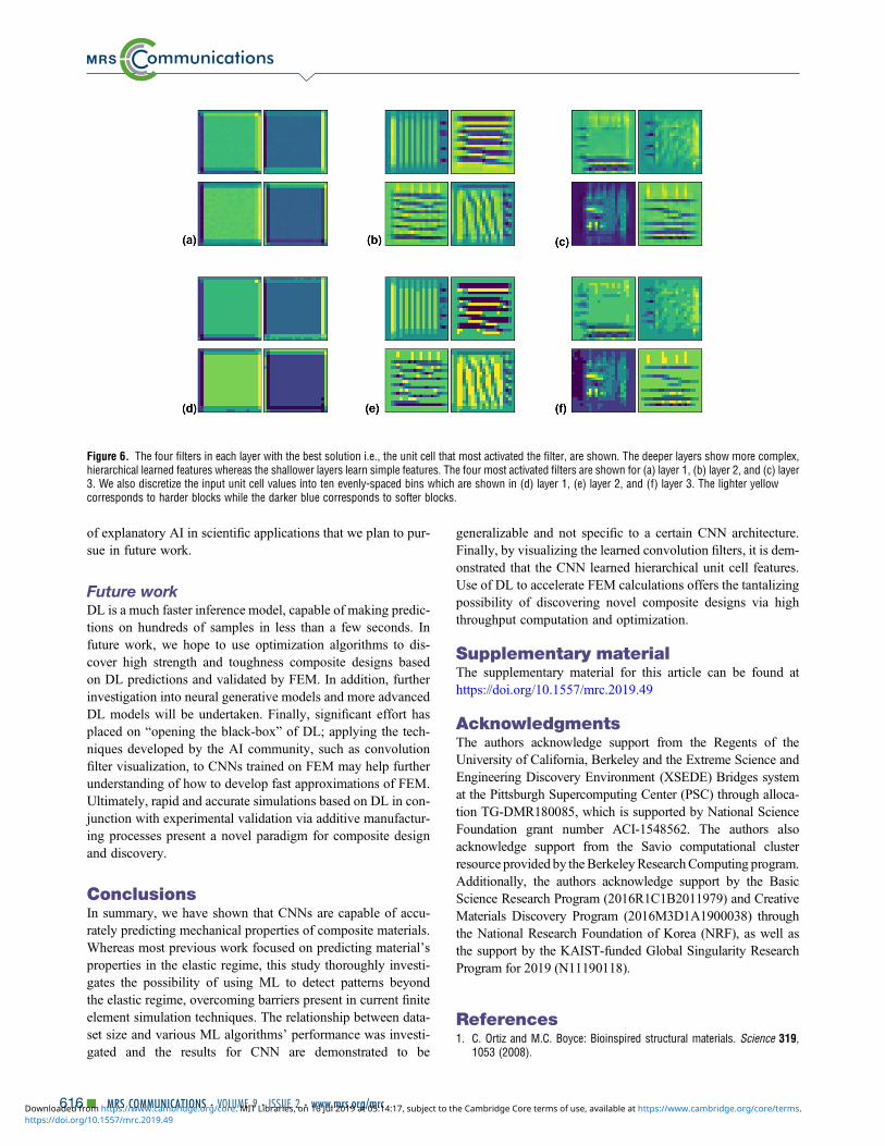
The learned convolution filters are shown in Fig. 6. The topfour filters in layer 1 are shown in Fig. 6(a), where each filter isranked according to the “best” solution found by the gradientoptimizer, the quality of the solution being measured by the

activation of the filter. The first layer is learning to detect simpleedges, mostly the right edge with hard blocks. The four mostactivated filters in layer 2 [Fig. 6(b)] have learned to detect hor-izontal and vertical stripes of alternating hard and soft blocks.Finally, layer 3 [Fig. 6(c)] has the most complex features. Itseems layer 3 has learned to detect grids of horizontal softblocks and vertical hard blocks and vice versa. The layer 3 con-volutions are the most complex and difficult to interpret as theyare compositions of the previous layer activations. The deeperlayers were also increasingly more difficult to optimize for; thegradient optimizer stopped due to the early stopping mecha-nism after a few iterations for the earlier layers but tookmany more iterations to stop for later layers. In Figs. 6(d)–6(f), we discretize the input unit cell values into ten evenlyspaced bins to simplify the visualization and make certain fea-tures clearer.

As hypothesized, the learned filters are radically differentfrom those learned for traditional image classification.However, the input cells that most activate each filter in thesequential layers of the CNN still exhibit the hierarchical learn-ing of features that is characteristic of CNNs; in our case, fromedges, to stripes, to alternating grids. Using visualization tech-niques developed by the AI community to explore how CNNslearn to predict various material properties (modulus, strength,and toughness) and how their learning is affected by FEM sim-ulation experimental parameters (crack direction and orienta-tion, composite design constraints) is an unexplored avenue

Figure 5. (a) Comparing the distribution of performance of CNN across 15 trials with just a unit cell input versus with unit cell input and the associated modulusvalue at predicting strength. The violin plots are kernel density estimates, which generate smoothed histograms from a given distribution. The metrics used arethe MAE, MSE, and R2 which is the square of the Pearson correlation coefficient. These models were evaluated with a 50/50 train/test split to better represent asmaller dataset size. (b) The distribution of modulus values by ranking as predicted by different CNN architectures. “Base model” is the overall CNN architectureused against RF and OLS. “Base model without BatchNorm” is the base model but with all batch normalization layers removed. “More convolution layers” is thebase model without max pooling layers and an extra Conv2D layer. “More dense layers” is the base model but with an extra dense layer at the end. Slightalterations were made to kernel and pool size to keep similar number of parameters for all models.






of explanatory AI in scientific applications that we plan to pur-sue in future work.

Future workDL is a much faster inference model, capable of making predic-tions on hundreds of samples in less than a few seconds. Infuture work, we hope to use optimization algorithms to dis-cover high strength and toughness composite designs basedon DL predictions and validated by FEM. In addition, furtherinvestigation into neural generative models and more advancedDL models will be undertaken. Finally, significant effort hasplaced on “opening the black-box” of DL; applying the tech-niques developed by the AI community, such as convolutionfilter visualization, to CNNs trained on FEM may help furtherunderstanding of how to develop fast approximations of FEM.Ultimately, rapid and accurate simulations based on DL in con-junction with experimental validation via additive manufactur-ing processes present a novel paradigm for composite designand discovery.

ConclusionsIn summary, we have shown that CNNs are capable of accu-rately predicting mechanical properties of composite materials.Whereas most previous work focused on predicting material’sproperties in the elastic regime, this study thoroughly investi-gates the possibility of using ML to detect patterns beyondthe elastic regime, overcoming barriers present in current finiteelement simulation techniques. The relationship between data-set size and various ML algorithms’ performance was investi-gated and the results for CNN are demonstrated to be

generalizable and not specific to a certain CNN architecture.Finally, by visualizing the learned convolution filters, it is dem-onstrated that the CNN learned hierarchical unit cell features.Use of DL to accelerate FEM calculations offers the tantalizingpossibility of discovering novel composite designs via highthroughput computation and optimization.

Supplementary materialThe supplementary material for this article can be found athttps://doi.org/10.1557/mrc.2019.49

AcknowledgmentsThe authors acknowledge support from the Regents of theUniversity of California, Berkeley and the Extreme Science andEngineering Discovery Environment (XSEDE) Bridges systemat the Pittsburgh Supercomputing Center (PSC) through alloca-tion TG-DMR180085, which is supported by National ScienceFoundation grant number ACI-1548562. The authors alsoacknowledge support from the Savio computational clusterresource provided by theBerkeleyResearchComputing program.Additionally, the authors acknowledge support by the BasicScience Research Program (2016R1C1B2011979) and CreativeMaterials Discovery Program (2016M3D1A1900038) throughthe National Research Foundation of Korea (NRF), as well asthe support by the KAIST-funded Global Singularity ResearchProgram for 2019 (N11190118).

References1. C. Ortiz and M.C. Boyce: Bioinspired structural materials. Science 319,

1053 (2008).

Figure 6. The four filters in each layer with the best solution i.e., the unit cell that most activated the filter, are shown. The deeper layers show more complex,hierarchical learned features whereas the shallower layers learn simple features. The four most activated filters are shown for (a) layer 1, (b) layer 2, and (c) layer3. We also discretize the input unit cell values into ten evenly-spaced bins which are shown in (d) layer 1, (e) layer 2, and (f) layer 3. The lighter yellowcorresponds to harder blocks while the darker blue corresponds to softer blocks.







2. U.G.K. Wegst, H. Bai, E. Saiz, A.P. Tomsia, and R.O. Ritchie: Bioinspiredstructural materials. Nat. Mater. 14, 23 (2015).

3. H.D. Espinosa, J.E. Rim, F. Barthelat, and M.J. Buehler: Merger of struc-ture and material in nacre and bone—perspectives on de novo biomi-metic materials. Prog. Mater. Sci. 54, 1059 (2009).

4. M.A. Meyers, J. McKittrick, and P-Y. Chen: Structural biological materials:critical mechanics-materials connections. Science 339, 773 (2013).

5. X. Wei, M. Naraghi, and H.D. Espinosa: Optimal length scales emergingfrom shear load transfer in natural materials: application to carbon-basednanocomposite design. ACS Nano 6, 2333 (2012).

6. G.X. Gu, F. Libonati, S.D. Wettermark, and M.J. Buehler: Printing nature:unraveling the role of nacre’s mineral bridges. J. Mech. Behav. Biomed.Mater. 76, 135 (2017).

7. F. Libonati, G.X. Gu, Z. Qin, L. Vergani, and M.J. Buehler: Bone-inspiredmaterials by design: toughness amplification observed using 3D printingand testing. Adv. Eng. Mater. 18, 1354 (2016).

8. Y. Kim, Y. Kim, T.I. Lee, T.S. Kim, and S. Ryu: An extended analytic modelfor the elastic properties of platelet-staggered composites and its applica-tion to 3D printed structures. Compos. Struct. 189, 27 (2018).

9. P. Tran, T.D. Ngo, A. Ghazlan, and D. Hui: Bimaterial 3D printing andnumerical analysis of bio-inspired composite structures under in-planeand transverse loadings. Composites, Part B 108, 210 (2017).

10.P. Zhang, M.A. Heyne, and A.C. To: Biomimetic staggered compositeswith highly enhanced energy dissipation: modeling, 3D printing, and test-ing. J. Mech. Phys. Solids 83, 285 (2015).

11.G.X. Gu, M. Takaffoli, and M.J. Buehler: Hierarchically enhanced impactresistance of bioinspired composites. Adv. Mater. 29, 1 (2017).

12.B. Ji and H. Gao: Mechanical properties of nanostructure of biologicalmaterials. J. Mech. Phys. Solids 52, 1963 (2004).

13.H. Jeong, S. Signetti, T.S. Han, and S. Ryu: Phase field modeling of crackpropagation under combined shear and tensile loading with hybrid for-mulation. Comput. Mater. Sci. 155, 483 (2018).

14.C. Miehe, M. Hofacker, and F. Welschinger: A phase field model for rate-independent crack propagation: robust algorithmic implementation basedon operator splits. Comput. Methods Appl. Mech. Eng. 199, 2765 (2010).

15.C. Miehe, F. Welschinger, and M. Hofacker: Thermodynamically consis-tent phase-field models of fracture: variational principles and multi-fieldFE implementations. Int. J. Numer. Methods Eng. 83, 1273 (2010).

16.H. Amor, J.J. Marigo, and C. Maurini: Regularized formulation of the var-iational brittle fracture with unilateral contact: numerical experiments. J.Mech. Phys. Solids 57, 1209 (2009).

17.C. Kuhn and R. Müller: A continuum phase field model for fracture. Eng.Fract. Mech. 77, 3625 (2010).

18.B. Bourdin, G.A. Francfort, and J.J. Marigo: The variational approach tofracture. J. Elast. 91, 5 (2008).

19.A. Krizhevsky, I. Sutskever and G.E. Hinton: ImageNet classification withdeep convolutional neural networks. Commun. ACM 60, 84 (2017).

20.Y. Lecun, Y. Bengio, and G. Hinton: Deep learning. Nature 521, 436(2015).

21.T. Jo, J. Hou, J. Eickholt, and J. Cheng: Improving protein fold recogni-tion by deep learning networks. Sci. Rep. 5, 1 (2015).

22.L. Wei and E. Roberts: Neural network control of focal position duringtime-lapse microscopy of cells. Sci. Rep. 8, 1 (2018).

23.M. Paganini, L. De Oliveira, and B. Nachman: CaloGAN: simulating 3Dhigh energy particle showers in multilayer electromagnetic calorimeterswith generative adversarial networks. Phys. Rev. D 97, 14021 (2018).

24.P.Z. Hanakata, E.D. Cubuk, D.K. Campbell, and H.S. Park: Acceleratedsearch and design of stretchable graphene kirigami using machine learn-ing. Phys. Rev. Lett. 121, 255304 (2018).

25.G.X. Gu, C.T. Chen, and M.J. Buehler: De novo composite design basedon machine learning algorithm. Extreme Mech. Lett. 18, 19 (2018).

26.G.X. Gu, C.T. Chen, D.J. Richmond, and M.J. Buehler: Bioinspired hierar-chical composite design using machine learning: simulation, additivemanufacturing, and experiment. Mater. Horiz. 5, 939 (2018).

27.L. Breiman: Random forests. Mach. Learn. 45, 5 (2001).28. F. Pedregosa, G. Varoquaux, A. Gramfort, V. Michel, B. Thirion, O. Grisel,

M. Blondel, P. Pretenhofer, R. Weiss, V. Dubourg, J. Vanderplas, A.Passos, D. Cournapeau, M. Brucher, M. Perrot, and E. Duchesnay:

Scikit-learn: machine learning in python. J. Mach. Learn. Res. 12, 2825(2011).

29. F. Chollet: Keras: the python deep learning library. Astrophysics SourceCode Library (2018).

30.D.P. Kingma and J. Ba: Adam: A method for stochastic optimization, inInternational Conference on Learning Representation (2015).

31.D. Erhan, Y. Bengio, A. Courville, and P. Vincent: Visualizing higher-layerfeatures of a deep network. Département d’Informatique Rech.Opérationnelle, Tech. Rep. 1341 No. 1341, 1 (2009).

32.Y. Nesterov: A method for solving the convex programming problem withconvergence rate O(1/k^2). Dokl. Akad. Nauk SSSR 269, 543 (1983).

33.B. Zoph and Q. Le: Neural architecture search with reinforcement learn-ing, in International Conference on Learning Representations (2017).

34.S. Ioffe and C. Szegedy: Batch normalization: accelerating network train-ing by reducing covariate shift, in International Conference on MachineLearning, edited by F. Bach and D. Blei (Proc. of Mach. Learn. Res. 37,Lille, France, 2015) p. 448.

35.M.D. Zeiler and R. Fergus: in Visualizing and understanding convolutionalNetworks, in European Conference on Computer Vision 2014, edited byD. Fleet, T. Pajdla, B. Schiele, T. Tuytelaars (13th European Conf. onComp. Vision 8689, Zurich, Switzerland, 2014), p. 818.






Using convolutional neural networks to predict composite properties beyond the elastic...

Documents

Transcript of Using convolutional neural networks to predict composite properties beyond the elastic...