Using concavity trees for shape description

Using concavity trees for shape descriptionB.G. Batchelor

Indexing terms: Graph theory, Pattern recognition

Abstract: The concavity tree (c.t.) is an attractive way of representing the shape of a 2-dimensional object orsilhouette. In this paper, the literature on the subject is briefly reviewed, the method of generating c.t.s isdescribed and their properties discussed. The paper goes on to report original work on the use of c.t.s formatching shapes and for detecting certain features such as edge features and symmetry. Possible applicationsof c.t.s are briefly reviewed, leading to the conclusion that they could be a valuable aid in the inspection,sorting and manipulation of industrial artefacts.

1 Introduction

Shape analysis is important in a number of fields of study,including reconnaissance, vehicle identification and,particularly, the inspection, sorting, measurement andmanipulation of certain types of industrial artefact. It isalso applied in other areas, although with perhaps lessjustification, particularly those in which the shapesassociated with a given class are highly variable, e.g. theletters of the alphabet as produced by different typewritersor chromosomes of a given group. A metal stamping,injection moulding, piece of leather for a shoe or cloth for asuit has a well defined shape; at least, it should have.Verifying this, or identifying the item, or locating a specifiednotch (or pip) on the edge, are tasks which the pictureanalyst is required to study if image-processing techniquesare to be applied in industry. Reference 1 gives a stimulatingaccount of this field. The tasks required for automaticinspection are summarised in the following list:

(a) Verify that a shape, made using a 'pastry cutter', hasbeen correctly manufactured (shape inspection).

(b) Determine the orientation of the shape (in a plane).(c) Determine whether the shape is 'heads up' or 'tails

up'. (Alternatively, is the shape left or right handed?)(d) Determine in which of its stable states a 3-dimensional

object has come to rest, after being dropped haphazardlyonto a table. (Like (e), this is an example of shape sorting.)

(e) Determine in which of a previously defined set ofcategories of shapes the given object lies (shape sorting).

(f) Identify a specified feature of the edge, as a preludeto picking up the object, or measuring that feature.A 'shape' may be regarded as a blob-like object, but it isimportant to note that, in view of its likely applications toindustrial tasks, shape analysis is concerned principally withobjects which are 'physically strong'. This is important,because it then becomes possible to use certain (fast)heuristic procedures which do not function properly onhighly convoluted edges, such as spirals which are physicallyweak. A shape may contain 'indentations' on its outer edgeand also 'holes', referred to by some authors2 as 'bays' and'lakes', respectively. Both holes and identations areexamples of 'concavities'.

The same methods may be used to describe theconcavities themselves as are applied to the original shape S.It is convenient therefore to use the term 'shape' to refer toany figure which is to be analysed. Later, we shall apply thesame methods of analysis to S, the concavities of S (both

Paper T395 C, first received 22 November 1978 and in revised form25th May 1979Dr. Batchelor is with the Department of Electronics, University ofSouthampton, Southampton S09 5NH, England

holes and indentations), concavities in its concavities('metaconcavities') and so on. It is possible to constructa concavity tree ct(5), which is an hierarchical descriptionof the given shape S. The concavity tree will be definedformally later, but let us first review the literature on thegeneral subject of shape analysis.

7.7 Literature

The earliest reference to concavity trees that the author hasyet encountered is that by Sklansky.3 Subsequently, workon this topic has been reported by Arcelli and Sanniti diBaja4 and Batchelor.s> 6> 7 The author is also aware of thework in this area by Dr. P. Zamperoni of the TechnischeUniversitat Braunschweig, FDR, but this has not yet beenpublished. The original suggestion by Sklansky was for aconcavity tree in which concavities were areas not coveredby the shape but covered by its 'convex hull'. Arcelli andSanniti di Baja4 employ a minimal-area irregular octagon,rather than the convex hull. Other possibilities exist (e.g.hexagons), but, to the author's knowledge, these have notbeen explored in earnest. Duda and Hart2 also realised thesignificance of concavities in shape description, but did notdevelop their ideas to encompass a recursive (tree-generating)algorithm. Pugh et al.8 developed Duda and Hart's ideasand applied them to the inspection of industrial components,while Rutovitz et al.9 applied similar ideas to microscopeimages of human chromosomes.

Other forms of hierarchical (tree-like) shape descriptionhave been proposed. See, for example, Montanari10 andPavlidis and Feng.11 It is not our intention here tocomment on the relative merits of their various methods.The literature on computing the convex hull of a given blobis reviewed separately in Section 2.1.1.

1.2 Outline of this article

We begin, in Section 2, by describing how a c.t. may begenerated. The subsidiary problem of computing theconvex hull is discussed in Section 2.1.1, and alternatives tothe convex hull are considered in Section 2.1.2. Theaddition of numeric shape descriptors to the tree isconsidered in Section 2.2. Tree pruning is discussed inSection 2.3.

Some of the properties of concavity trees are describedin Section 3. These include: instability of the tree (Section3.1); rotational invariance (and normalisation)(Section 3.2);handedness (and normalisation) (Section3.3); quantisation-noise effects (Section 3.4). In Section 4, some of the usesof concavity trees are discussed: shape matching (Section4.1); edge segmentation (Section 4.2; detecting specifiededge features (Section 4.3); detecting symmetry (Section

COMPUTERS AND DIGITAL TECHNIQUES, AUGUST 1979, Vol. 2, No. 4 157

0140-1335/791040157 + 12 $01-50/0

4.4). In Section 5, there follows a brief review of possibleapplications of concavity trees to the inspection, sortingand manipulation of industrial artefacts.

2 Generating concavity trees

2.1 Generating the basic tree5

Let(a) Pbea binary picture with n x n pixels.(b) S (C P) be the set of white points in P. We shall

assume that S is 8-connected; there is only one shape(a 'blob') provided initially.

(c) 8* denote the convex hull of an arbitrary connectedshape 0; both holes and indentations of 0 are Tilled' byforming 0*.

(d)Ci denote the region within the rth concavity; thatis

A T ,

s= u c,1=1

where the Q (/ = 1 , . . . , Nx) are 8-connected shapes, eachcovering either one hole or one indentation. Notice that

and C,-, Cj are not 8-connected to each other.(Here we see the importance of the assumption that theshape S is physically strong). We shall refer to the Q as'1-concavities' of 5, to distinguish them from other featuresdefined below.

Original

Meta-Meta-Concavities

b

Fig. 1 Drawing a concavity tree

a Shape 5b ct(5) and its relationship to the (convex hulls of the) m-

concavities of S

(e) each of the Q be represented by the union of a set of'metaconcavities' (or '2-concavities') which are cut fromthe convex hull of C,-; That is, the set of points

C* — C-

may be represented by an expression of the form

"i .U D)

;=i

where the D) are individually 8-connected, are disjointfrom each other and are not 8-connected to one another.'Metametaconcavities' lE'h and even 'higher-level' shapes(m-concavities) may be defined in a similar way.

We shall refer to concavities, metaconcavities, meta-metaconcavities etc. collectively as 'm-concavities'. By thisterm, we imply that the level of recursion (m) is uncertain.

(/) ct(5) be a tree whose root (Oth-level node) re-presents S*, whose first level nodes are* the C*, 2nd-levelnodes the (£>/)*, 3rd-level nodes the ('£&)*, and so on;ct(S) is termed the concavity tree of S.

Now, let us illustrate this process. Fig. \a shows a testshape; a polygon was chosen for simplicity of illustration.Fig. \b shows the concavity tree, ct(S). The thumbnailsketches beside the tree show the relationship between itsnodes and the various m-concavities of S. The tree may beregarded as a method of describing how S may be approxi-mated. The initial approximation is S* (node A). A betterapproximation can be obtained by 'cutting away' the1-concavities (nodes B, C and D) from S*. Furtherrefinements can be obtained by 'sticking back' the 2-concavities (nodes E, F, G and H). By cutting away the3-concavity (node J), the approximation becomes perfect.In general, 'odd-level' nodes (m = 1, 3, 5, 7 . . .) correspondto m-concavities which are cut-away, while 'even-level'nodes (m = 0, 2, 4, 6 , . . . ) are stuck back. The level ofrecursion (m) needed to obtain a perfect representation of ahighly convoluted input shape may be quite high. In general,though, physically strong shapes produce trees of moderatedepth (m < 5); several examples emphasising this point aregiven in this paper.

2.1.1 Deriving the convex hull:12 The simplest 'computer'for finding the edge of the convex hull 9* of a given shape 9is a rubber band. However, this is hardly practical for use inan electronic machine and so several algorithmic methodshave been proposed; these operate on the connected setthat represents 9. Considerable saving in computation timecan be achieved by first finding the edge of 9 andcomputing, not 9*, but the vertices of that polygon whichbounds 6*. Let NQ be the number of edge elements in 9;VQ* the number of vertices of that polygon bounding 9*and VQ the number of vertices is a polygonal approximationto the edge of 9. Nine methods for deriving the convex hullare commented on below. (In each case, it is assumed thatthe edge of 9, or a polygon approximating it, has alreadybeen found.):

(a) Arcelli and Levialdi:13 Very slow on a serial machine,but the method in a modified form is well suited to aparallel processor such as clip (Reference 14 and Section2.1.2)

(b) Rosenfeld and Kak:15 Two methods are described:one of them being that first defined by Arcelli and Levialdi,12

For linguistic convenience, we shall use the verb form 'is' ratherthan the more rigorous but cumbersome phrase 'is associated with'.

158 COMPUTERS AND DIGITAL TECHNIQUES, AUGUST 1979, Vol. 2, No. 4

and the other is slow. (It is difficult to estimate thecomputation time in quantitative terms).

(c) Rutovitz etal: Apparently requires time O(Ne-Ve*)(d) Graham:16 Requires O(Nd \ogN0) time(e) Jarvis:17 Requires O(NQ) time(/) Batchelor and Laing:18 Two techniques are presented.

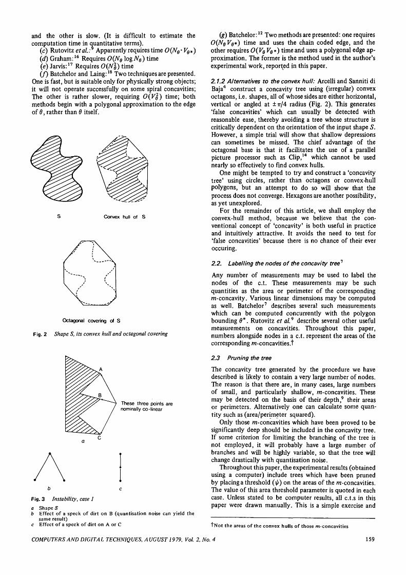
One is fast, but is suitable only for physically strong objects;it will not operate successfully on some spiral concavities;The other is rather slower, requiring O(VQ) time; bothmethods begin with a polygonal approximation to the edgeof 0, rather than 0 itself.

Convex hull of S

Octagonal covering of S

Fig. 2 Shape S, its convex hull and octagonal covering

These three points arenominally co-linear

Fig. 3 Instability, case 1

a Shape Sb Effect of a speck of dirt on B (quantisation noise can yield the

same result)c Effect of a speck of dirt on A or C

(g) Batchelor:12 Two methods are presented: one requires0{NQVQ*) time and uses the chain coded edge, and theother requires O(Ve Ve*) time and uses a polygonal edge ap-proximation. The former is the method used in the author'sexperimental work, reported in this paper.

2.1.2 Alternatives to the convex hull: Arcelli and Sanniti diBaja4 construct a concavity tree using (irregular) convexoctagons, i.e. shapes, all of whose sides are either horizontal,vertical or angled at ±TT/4 radius (Fig. 2). This generates'false concavities' which can usually be detected withreasonable ease, thereby avoiding a tree whose structure iscritically dependent on the orientation of the input shape S.However, a simple trial will show that shallow depressionscan sometimes be missed. The chief advantage of theoctagonal base is that it facilitates the use of a parallelpicture processor such as Clip,14 which cannot be usednearly so effectively to find convex hulls.

One might be tempted to try and construct a 'concavitytree' using circles, rather than octagons or convex-hullpolygons, but an attempt to do so will show that theprocess does not converge. Hexagons are another possibility,as yet unexplored.

For the remainder of this article, we shall employ theconvex-hull method, because we believe that the con-ventional concept of 'concavity' is both useful in practiceand intuitively attractive. It avoids the need to test for'false concavities' because there is no chance of their everoccuring.

2.2. Label/ing the nodes of the concavity tree1

Any number of measurements may be used to label thenodes of the c.t. These measurements may be suchquantities as the area or perimeter of the correspondingm-concavity. Various linear dimensions may be computedas well. Batchelor7 describes several such measurementswhich can be computed concurrently with the polygonbounding 0*. Rutovitz et al.9 describe several other usefulmeasurements on concavities. Throughout this paper,numbers alongside nodes in a c.t. represent the areas of thecorresponding ra-concavities.t

2.3 Pruning the tree

The concavity tree generated by the procedure we havedescribed is likely to contain a very large number of nodes.The reason is that there are, in many cases, large numbersof small, and particularly shallow, m-concavities. Thesemay be detected on the basis of their depth,9 their areasor perimeters. Alternatively one can calculate some quan-tity such as (area/perimeter squared).

Only those m-concavities which have been proved to besignificantly deep should be included in the concavity tree.If some criterion for limiting the branching of the tree isnot employed, it will probably have a large number ofbranches and will be highly variable, so that the tree willchange drastically with quantisation noise.

Throughout this paper, the experimental results (obtainedusing a computer) include trees which have been prunedby placing a threshold (i//) on the areas of the w-concavities.The value of this area threshold parameter is quoted in eachcase. Unless stated to be computer results, all c.t.s in thispaper were drawn manually. This is a simple exercise and

TNot the areas of the convex hulls of those /n-concavities


the reader is encouraged to try this for himself, to gainfamiliarity with the methods.

These edges arenominally aligned

Largearea Very small

area

Largearea

Large Largearea area

theoretical treatment of blobs, seem to be of no greatimportance. However, certain human artefacts (some metalstampings, mouldings, pressings etc.), do have such featuresand, as a result, the c.t.s of these objects should not be usedwithout great care. The stampings shown in Fig. 5 are 'safe',whereas others, such as the E-shaped stamping for atransformer core, are not.

Large Largearea area

Fig. 4 Instability, case 2

a Shape Sb Edges AC and BD aligned exactly (the same tree results if AC

and BD, when produced, meet at an obtuse angle)c Effect of a speck of dirt on A or Bd Edges AC and BD, when produced, meet at a reflex angle, (other

tree forms are possible by very small distortions of S)

3 Some properties of concavity trees

3.1 Instability

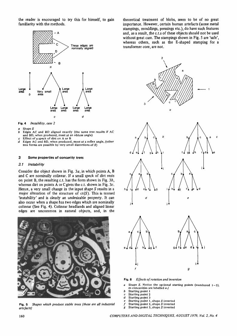
Consider the object shown in Fig. 3a, in which points A, Band C are nominally colinear. If a small speck of dirt restson point B, the resulting c.t. has the form shown in Fig. 3b,whereas dirt on points A or C gives the c.t. shown in Fig. 3c.Hence, a very small change in the input shape S results in amajor alteration of the structure of c t ^ ) . This is termed'instability' and is clearly an undesirable property. It canalso occur when a shape has two edges which are nominallycolinear (See Fig. 4). Colinear headlands and aligned linearedges are uncommon in natural objects, and, in the

Fig. 6 Effects of rotation and inversion

Fig. 5 Shapes which produce stable trees (these are all industrialartefacts)

Shape S. Notice the optional starting points (numbered 1—3).m-concavities are labelled a-jStarting point 1Starting point 2Starting point 3Starting point 1, shape 5 invertedStarting point 2, shape S inverted


How can instability be overcome? There does not appearto be any simple algorithmic solution, nor is there anyknown heuristic which is robust enough for general use.One possible approach is to accept that instability willoccur and store reference trees for each of the possiblestructures that might be found. Although this results in anincrease in the storage required, this is probably ofrelatively minor importance, because the trees obtained inpractice are normally quite small (see, for example, Fig. 8).However, by storing two (or more) archetypal trees toaccomodate instability, the tree-matching time (Section 4.1)is effectively doubled. For this reason, the author is stilltrying to develop ways of avoiding instability, rather thanmerely accomodating it after it has happened.

3.2 Rotational invariance and normalisation

The concavity tree generated by the procedure describedabove is in most respects, but not entirely, rotationallyinvariant (see Fig. 6). However, the following simplenormalising procedure is effective for nearly all shapes:

Measure the area of each 1-concavity and select thatnode corresponding to the 1-concavity with the greatestarea. This node is the one that is then drawn on the left ofthe tree. The remaining first-level nodes are then drawn inturn, taking them in the same (cyclic) order as they appearin the nonnormalised tree.

Unfortunately, some shapes possess two large 1-concavities which have roughly the same area. Afterdigitisation, quantisation noise may render their areaestimates so imprecise that their rank order is reversed.Thus, we must be prepared to use some other criterion forachieving normalisation. Some possible shape descriptorsfor doing this are discussed by Batchelor7 and Rutovitzetal.9

3.3 Shape inversion (handedness)

Fig. 6 shows the effects of inverting the input shape (i.e.turning it over, or exchanging it for its mirror image). Thetree is unchanged except that, for a given start point, itsleft-right ordering is reversed (compare Figs. 6b, and 6e,6c and 6f, 6d and 6g). The question to which we shalladdress ourselves now is that of determining the 'handedness'of a shape from its associated concavity tree. It is possibleto do this, in many cases, without storing and matching areference tree to ct (5). For instance, a possible procedure,illustrated on the shape in Fig. 6a, is as follows. Here, Ad

and Ae represent the areas of 2nd-level concavities d and e,respectively, and Ad and Ae represent the correspondingestimated areas after digitisation. The steps in theprocedure are:

(a) Digitise the shape S and derive ct (S).(b) Normalise ct(S) for the effects of rotation. (The

result of this operation on Fig. 6a would be to yield atree having the form of Fig. 6b or Fig. 6/.)

(c) Find the two left-most nodes in level 2 [(d) and (e)]which are pendant from the left-most node in level 1.Estimate the areas of the corresponding 2-concavities, Ad

andAe.(d) We (arbitrarily) define a 'right-handed' shape S to be

one whose rotation-normalised concavity tree ct(S) hasnodes d and e in the second level such that Ad>Ae,whereas node d lies to the left of e. Thus, Figs 6b-dcorrespond to the right-handed shape and Figs. Se-g to itsmirror image (a left-handed shape).

Now, this procedure is satisfactory for all shapes havingtwo or more m-concavities (m > 2) associated with the1-concavity which has the largest area. Clearly, some shapesdo not possess this property. In this case, we could comparethe areas of two predefined 1-concavities and use the resultto test for handedness. Clearly, this is not universal either,because this requires that there be at least three 1-concavities.Thus, we are forced to the conclusion that handedness canonly be determined from ct(S") if the form of input shapeS is known i.e. how many 1-concavities, 2-concavitiesetc. there are.

Another problem with the above procedure is that incases where Ad and Ae are roughly equal, quantisationnoise may give a false impression as to which of them isthe larger.

Despite these difficulties, the determination of thehandedness of a limited class of shapes is not likely to causeserious problems in practice. Let us reflect, for the moment,why the determination of handedness is important.Consider the problem of sorting shaped laminate objectswhich are tossed haphazardly onto a conveyor belt, beforescanning, digitisation and routing to one of a number ofboxes.19 It is not difficult to see that the sorting processrequires half the storage and half the processing time, if thehandedness of the test shape and all of the stored reference-shapes can be determined immediately they are generated.

Fig. 7 Showing the effects of quantisation noise (experimentalresults)

a Shape S (notice the digitisation)b ct (S) after rotation normalisationc ct (S) (before redigitisation, S was rotated by 90°, ct has been

normalised for rotation)d ct (S) (before redigitisation, S was rotated by 270°, the ct has

been normalised for rotation)


3.4 Quantisation noise

The effects of quantisation noise on the tree representinga shape in different rotational and/or translational positionsare twofold. When the nodes of the c.t. are labelled with theareas of the corresponding concavities, different positionscan result in different estimated areas. Another effect,seen after tree pruning has taken place, is that in somerotational positions a branch of the c.t. will be insignificantenough to be removed, whereas in other positions it will beleft. Thus, as the rotational position of a shape is changed,the c.t. can vary as to its structure and the labelling of itsnodes. The extent of these effects in a typical case is shownin Fig. 7.

4 Using concavity trees

4.1 Shape matching

If there were no quantisation noise, the matching ofconcavity trees would be a trivial exercise, involving only

(a) normalisation, for rotation and handedness(b) overlaying the two trees, which should be identical,if their corresponding shapes are identical.

In practice, however, the two (normalised) trees are un-likely to be identical for two reasons; the shapes may notbe identical, but 'similar' and quantisation noise mayproduce quite significant changes in the tree structure(Section 3.4). For this reason, an algorithm taking accountof these differences has been devised; it is set out inAppendix 8. The results of using this algorithm on somesimple concavity trees are presented in Fig. 8, where it maybe seen that the procedure has correctly matched the majorfeatures. Attempting to match two different shapes usuallyresults in the match being poor.

(43) i

Fig. 8 Shape matching of the same object in three orientations(experimental results)

a c.t.s in Pigs. 1c and Id matched. Numbers indicate area-differenceand square nodes and dotted arcs unmatched m-concavities

b c.t.s in Figs. 76 and Id matched

4.2 Segmenting the edge

Consider Fig. 9a. The arc ABCD and the straight line DAtogether bound a concavity. The points A and D areexamples of what we shall term 'e-points' (e for 'ends ofthe arc'). The tree in Fig. 9b has its nodes labelled by listingthe e-points for each m-concavity. A c.t. generator iseffectively a procedure for calculating e-points; it is thusperfectly natural to regard the generator as a means ofsegmenting the periphery of the given figure. Notice thatthe e-points are not necessarily points of high curvature,whereas this is the usual requirement for an edge-segmentingalgorithm.15 (The e-points A, D, E and M are best regardedas being 'headlands').

Using the e-points as a basis for segmenting the edge, itis possible to 'punctuate' the edge code (e.g. the 'chain code'),in such a way that the positions of the e-points and the treestructure are both evident. This process may be likened to'un-parsing' the c.t. The idea is outlined in Appendix 8.2.

Start

GH JK

Fig. 9 Edge segmentation, e-points and edge-feature location

a Shape S. Capital letters denote e-points; lower-case 'x' denotes aconvex arc and iv' a concave arc

b ct(5). The nodes are labelled with the e-points which delimitthe corresponding m-concavity

4.3 Detecting specified edge features

Suppose that we have been given a shape S in randomorientation and that, by constructing ct (S) and matchingthat with its (various) ideal(s), we have verified that S is arecognisable object. The (best-fit) archetypal tree c.t.A isassumed to have a predefined m-concavity of interest.Perhaps this is a rather critical region which requires specialmeasurements to be made on it; to do so, it must first belocated. We have already seen how a given node in a c.t.may be associated with a well defined region of the edge;the e-points, defined in Section 4.2, are central to thisprocess, because they provide a relatively precise methodof locating the m-concavity. The following steps arerequired:

(i) Identify the special node N of the ideal concavitytree c.t.^.

(ii) Draw the concavity tree of S, ct(5)(iii) Match ct(S) to c.t.^; for each node in ct(S), find

the corresponding node in c.t.A.(iv) Find that node in ct(5) which matches node N.

Denote this by V.


(v) Find the e-points of that m-concavity in S whichcorresponds to V.

Root

t,' (sub-tree t, reversed)

Symmetrical concavity

Fig. 10 Symmetry

Symmetrical concavity(bisected by the axis of symmetry)

General form of the c.t. of a shape with a single axis of symmetry.Some of the subtrees may be 'null' (no nodes). t\ is that subtreeobtained by reversing the left-right ordering of the subtree f,-f, , 1-concavity plus its internal m-concavitiest2, 2-concavity plus its internal m-concavitiest3, 2-concavity plus its internal m-concavities

In theory, establishing symmetry or periodicity is fairlystraightforward, but, in practice, there are complications,owing to the effects of quantisation noise. Detectingsymmetry of a shape with n 1-concavities requires matchingthe original tree c.t. with n trees, c.t.J, where the primedenotes tree inversion (left-right ordering reversed) andthe subscript / denotes a rotational shift by /1-concavities.Periodicity should, in the ideal case, result in the generationof m 'identical' subtrees, all pendant from the root, wherethe (rotational) period is given by 2n/m. This fact may beused to good effect in reducing the amount of storagerequired for archetypal c.t.s. It also suggests an algorithmfor detecting m-fold rotational periodicity. All m lst-levelnodes should match; all second-level nodes should havera-1 matching nodes, and similarly for higher levels of thec.t. In practice, however, the task is far from simple;quantisation noise makes the c.t. 'ragged' (see Fig. 12).We have not yet developed a solution to the practicalproblems that quantisation noise brings.

Fig. 11 Shape with two axes of symmetry (experimental result)

a Metal-stamping edge (inner edge of a stator laminate for anelectric motor)

b ct.

4.4 Symmetry and rotational periodicity

Symmetry and rotational periocicity in the input shape Sare both manifest in ct (S) in a fairly obvious way. Fig. 10presents the general c.t. for a shape with one axis ofsymmetry, similar features being found when the numberof axes of symmetry is greater. Computer-derived c.t.s forshapes with 2 and several axes of symmetry are shown inFigs. 11 and 12, respectively. Notice the effects of quanti-sation noise in these two Figures.

Fig. 12 Multiple symmetry

a Metal-stamping edge (outer edge of the rotor laminate which'mates' with the shape in Fig. la). The e-points delimiting the1-concavities have been highlighted

b c.t.; the tree was truncated with an area threshold parameter \pof 10


Fig. 13 Automatic visual inspection of a metal stamping

Edgec.t.; the small 1-concavities (A, B and C) are cut out by pin-likeprotrusions on the punch head. Breakage of one of these wouldresult in the deletion of the corresponding node from the c.t.(Area threshold parameter \}J = 25)

5 Discussion

5.7 Applications

Concavity trees have been studied by the author in thehope that they can be used for the automatic visualinspection of industrial artefacts. Parks1 gives a goodgeneral account of this area of research, and Batchelors> 6

describes the use of concavity trees for the inspection andsorting of 'flat' industrial artefacts (i.e. those which canusefully be viewed in silhouette). The following tasksmight benefit from the use of concavity trees as shaperepresentation:

(a) Detection of severe local defects in the silhouettes offlat objects (Fig. 13)Components which have only two stable states (e.g. metalpressings, stampings and certain flat moulded objects) fallin the category of objects which might be inspected bystudying the concavity trees of their silhouettes. For thisapplication, the following tree properties would be

important:(i) rotation invariance (achieved, of course, by normal-

ising the trees)(ii) handedness invariance (again, achieved by normal-

ising the trees)(iii) the systematic use of qualitative (shape) and quanti-

tative (metric) data(iv) identification of specific edge features for special

measurements of critical regions of the object(v) tree matching and comparison

(b) Sorting of shapes (Fig. 14)The sorting of shapes might be employed in the clothingand leather industries, where large numbers of irregularlyshaped flat components are cut by an operator from thefeed material. For various reasons, these components arejumbled together, and must be sorted before machining.In this application, the following properties would beimportant:

(i) rotation invariance(ii) handedness identification (to distinguish between

left and right components)(iii) size invariance(iv) low data requirements of the archetype trees which

have to be sorted for use in the sorting process(v) tree-matching speed (to speed up this process, it

may be necessary to sort the archetype trees into groups ofsimilar type)

(c) Recognition of posture of 3-dimensional objects(Fig. 15)Many 3-dimensional objects have a small number of stableresting states, which are distinguishable from their sil-houettes. The recognition of posture is thus a problem ofsorting shapes.

(d) Calculating gripping points for object manipulationConsider that class of thick plate-like objects whosesilhouettes resemble the blobs we have been discussing inthis paper. It is possible to lift such a plate from a table-top,by judiciously placing the fingers of a 3-finger gripper in itsconcavities. Clearly some grips are unstable; the safest gripsare those in which the centre of the object lies within thetriangle formed by the fingers. Suitable gripping positionscould be calculated using the method discussed in Section4.3. It is impossible to do justice to this important topic inthe small space available here. Let it suffice to point outthat the calculation of gripping points is made much easierif the objects to be lifted are known beforehand. Thisallows preprogramming by the robot designer, who caneasily determine safe lifting points, if he sees the objectsbefore the robot does.

5.2 Unanswered questions

The concavity tree is only one of a number of shaperepresentations. It would be interesting to relate these toone another, and, in particular, to find some method ofderiving Pavlidis and Feng's polygonal decomposition,11 orthe medial-axis transformation,10 from the concavity tree,and vice versa. It is also important to establish somecriterion for deciding which of these shape representationsis most suitable for use in a given application. Anotherunanswered question is how to avoid the kind of instabilitydescribed in Section 3.1. The central computation inderiving the concavity tree is that of finding the convex hull


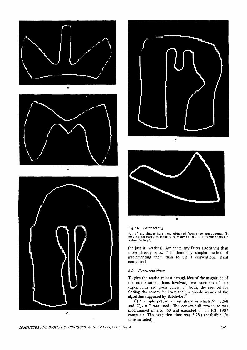
Fig. 14 Shape sorting

All of the shapes here were obtained from shoe components. (Itmay be necessary to identify as many as 10 000 different shapes ina shoe factory!)

(or just its vertices). Are there any faster algorithms thanthose already known? Is there any simpler method ofimplementing them than to use a conventional serialcomputer?

5.3 Execution times

To give the reader at least a rough idea of the magnitude ofthe computation times involved, two examples of ourexperiments are given below. In both, the method forfinding the convex hull was the chain-code version of thealgorithm suggested by Batchelor.12

(i) A simple polygonal test shape in which TV = 2268and Ve*=7 was used. The convex-hull procedure wasprogrammed in algol 60 and executed on an ICL 1907computer. The execution time was 5-78 s (negligible i/otime included).


Fig. 15 Recognition of component posture

a Outline of a small toggle switch in three of its stable postures.(There are six altogether)

b Concavity trees for the shapes in (a)

*

10

50

10-0

200

500

Timeseconds

125

109

103

103

097

Fig. 16 Concavity-tree and program execution times for shapeshown in Fig. 14c

a ct(iS) for area-threshold parameter i// = 10b Execution times for various values of t//

(ii) In this example, the complete concavity-treegenerator was programmed in Fortran IV and executed on aModcomp IV minicomputer. The test shape was that shownin Fig. 14c, and its concavity tree, together with theexcution times, are given in Fig. 16.

6 Conclusions

In this paper, the author has attempted to develop theunderstanding and use of concavity trees in industrialinspection, for which they seem to be very well suited. Aconcavity tree is a convenient method of shape descriptionwhich allows metrical and qualitative data about the shapeto be assimilated in a systematic structure. Both local andglobal information can be incorporated into a single tree.Concavity trees exhibit some useful properties, particularlyfor determining object orientation, handedness andspecified edge features. A tree-matching algorithm has beendefined and demonstrated on simple examples. Althoughconcavity trees suffer from instability, for example whenthe input shape has the form of a letter 'E', this is unlikelyto be a nuisance in practice. The possible application ofconcavity trees to industrial inspection, shape sorting androbotics has been emphasised, and it is clear that this formof shape description closely matches the requirements ofa system for examining and handling objects viewed insilhouette.

7 References

1 PARKS, J.R.: 'Industrial sensory devices', in Batchelor, B.G.(Ed.): 'Pattern recognition: ideas in practice' (Plenum, NewYork, 1978)

2 DUDA, R.O., and HART, P.E.: 'Pattern classification and sceneanalysis' (Wiley-Interscience, New York, 1973)

3 SKLANSKY, J.: 'Measuring concavity on a rectangular mosaic',IEEE Trans, 1972, C-21, pp. 1355-1364

4 ARCELLI, C, and SANNITI di BAJA, G.: 'Polygonal coveringand concavity trees of binary digital pictures'. Procedings MECO'78, published by Panhellenic Society of Mechanical & ElectricalEngineers, Athens, Greece, pp. 292-297

5 BATCHELOR, B.G.: 'Shape description using concavity trees',Proceedings MECO '78, published by Panhellenic Society ofMechanical & Electrical Engineers, Athens, Greece, pp. 385—390

6 BATCHELOR, B.G.: 'Hierarchical shape description based uponthe convex hulls of concavities' (accepted for publication in/. Cybern., draft copies available from the author)

7 BATCHELOR, B.G.: 'Shape descriptors for labelling concavitytrees' (accepted for publication in J. Cybern., draft copiesavailable from the author)

8 PUGH, A., WADDON, K., and HEGINBOTHAM, W.B.: 'Micro-processor controlled photodiode sensor for the detection ofgross defects'. Proceedings 3rd International Conference onAutomated Inspection and Product Control, Published by Inter-national Fluidics Services, Kempston, England and IITRI,Chicago, USA, pp. 229-312

9 RUTOVITZ, D., GREEN, D.K., FARROW, A.S.J., and MASON,D.C.: 'Computer assisted measurement in the cytogeneticlaboratory', in Batchelor, B.G. (Ed.): 'Pattern recognition: ideasin practice' (Plenum, New York, 1978)

10 MONTANARI, U.: 'Continuous skeletons from digital pictures',/. ACM, 1969, 16, pp. 534-549

11 PAVLIDIS, Th., and FENG, H.-Y. F.: 'Shape discrimination', inFu, K.S. (Ed): 'Syntactic pattern recognition, applications'(Springer-Verlag, Berlin, 1977)

12 BATCHELOR, B.G.: 'Two methods for finding convex hulls ofplanar figures' (accepted for publication in the J. Cybern., draftcopies available from the author)

13 ARCELLI, C, and LEVIALDI, S.: 'Concavity extraction byparallel processing', IEEE Trans., 1971, SMC-1, pp. 394-396

14 DUFF, M.J.B.: 'Parallel processing techniques', in Batchelor,B.G. (Ed.): 'Pattern recognition, ideas in practice' (Plenum,New York, 1978)


15 ROSENFELD, A., and KAK, A.C.: 'Digital picture processing'(Academic Press, New York, 1976)

16 GRAHAM, R.L.: 'An efficient algorithm for determining theconvex hull of a finite planar set', Inf. Process. Lett, 1972, 1,pp. 132-133

17 JARVIS, R.A.: 'On the identification of the convex hull of afinite set of points in the plane', ibid., 1973, 2, pp. 18-21

18 BATCHELOR, B.G., and LAING, S.G.: 'Polar vector represen-tations of edges in pictures', Electron. Lett, 1977,13, p. 727

19 BROWN, A.: The orientation of components for automaticassembly' (in preparation)

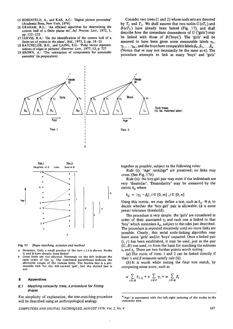
Consider two trees (1 and 2) whose node sets are denotedby Tx and T2. We shall assume that two nodes G (eTi) andB(eT2) have already been linked (Fig. 17), and shalldescribe how the immediate descendents of G ('girls') maybe linked with those of 2? ('boys'). The 'girls' will beassumed to have been given some measurable labels y0,7 i , . . . ym, and the boys have comparable labels j30, 0 i , . . . 0n.(Notice that m may not necessarily be the same as n). Theprocedure attempts to link as many 'boys' and 'girls'

ft,

Sub-trees(to be matched later)

Age

Tree 2

Tree 1

Daughters' of G

Tree 2

Sons'of B

Fig. 17 Shape matching, notation and method

a Notation. Only a small portion of the two c.t.s is shown. NodesG and B have already been linked

b Cross links are not allowed. Numerals on the left indicate therank order of the 7,-. The numbered parantheses indicate theallowable ranges of the various links. The broken line is a per-missible link for the 4th-ranked 'girl', but the dotted line isnot

8 Appendixes

8.1 Matching concavity trees, a procedure for fittingshapes

For simplicity of explanation, the tree-matching procedurewill be described using an anthropological analogy.

together as possible, subject to the following rules:Rule (i): 'Age' rankings* are preserved; no links may

cross. (See Fig. lib)Rule (ii): No boy-girl pair may exist if the individuals are

very 'dissimilar'. 'Dissimilarity' may be measured by themetric 5,-y where

b~tj = 17,- — j3;|, /' G [0, m],/ £ [0, n]

Using this metric, we may define a test, such as 6# ^ 0, todecide whether the 'boy-girl' pair is allowable. (0 is somepreset tolerance threshold).

The procedure is very simple: the 'girls' are considered inorder of their associated 7,- and each one is linked to that'boy' which minimises 5i;-, subject to the rules just described.The procedure is repeated iteratively until no more links arepossible. Clearly, this serial node-linking algorithm mayleave some 'girls' and/or 'boys' unpaired. Once a linked pair(i, / ) has been established, it may be used, just as the pair(G, B) was used, to form the basis for matching the subtreesSi and tj. There are two further points worth noting:

(a) The roots of trees 1 and 2 can be linked directly iftheir 7 and |3 measures satisfy rule (ii).

(b) It is worth while testing the final tree match, bycomputing some score, such as

u Z Si ;•• + v Z Ii + w Z $jiGP ;GQ

*'Age' is associated with the left-right ordering of the nodes in theconcavity tree.


where(a) (i, ji) is the general linked pair (zth 'girl', /,-th 'boy')

and R is the set of such linked pairs.(b) P is the set of unlinked 'girls' in tree 1(c) Q is the set of unlinked 'boy' in tree 2(d)u,v and w are weighting coefficients.

Low values of this score indicate a good fit. This score mayalso be used as a measure of the similarity of the shapesrepresented by the two trees.

If the trees have their nodes labelled by measurementvectors, then a more sophisticated shape-similarity measuremay be useful. One possibility is described below. Let x{ de-note the label associated with the ithnode in tree 1, (/ G 7\)and yj that associated with the /th node in tree 2 ( / £ T2).(Both x{ and yj are, say, ^-dimensional vectors). Then, apossible shape-matching score is given by

\\yj\\u y II*.—v-n + 0 y II*-H + -iGR tep

8.2 Punctuating the edge coding of a shape

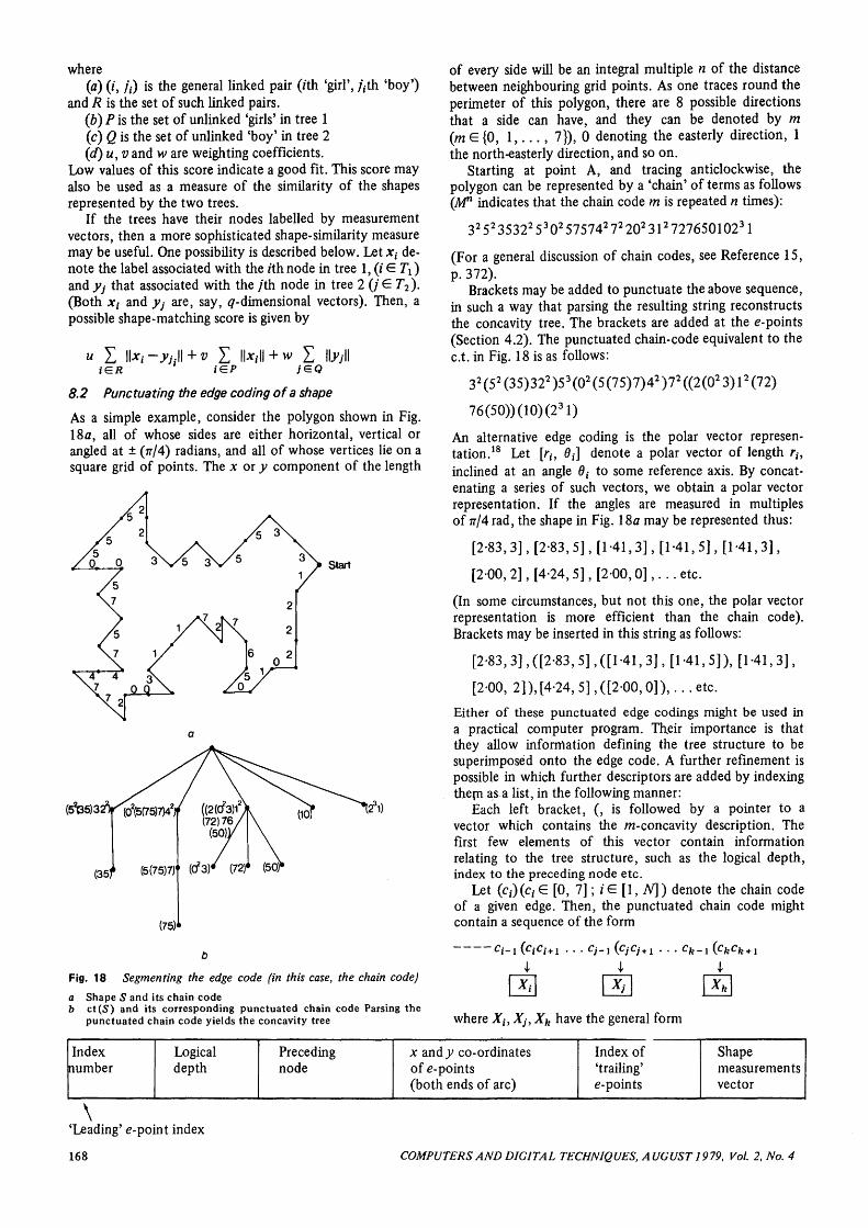
As a simple example, consider the polygon shown in Fig.18fl, all of whose sides are either horizontal, vertical orangled at ± (n/4) radians, and all of whose vertices lie on asquare grid of points. The x or y component of the length

Start

(5^05)3

Fig. 18 Segmenting the edge code (in this case, the chain code)

a Shape S and its chain codeb ct(5) and its corresponding punctuated chain code Parsing the

punctuated chain code yields the concavity tree

of every side will be an integral multiple n of the distancebetween neighbouring grid points. As one traces round theperimeter of this polygon, there are 8 possible directionsthat a side can have, and they can be denoted by m(m G {0, 1 , . . . , 7}), 0 denoting the easterly direction, 1the north-easterly direction, and so on.

Starting at point A, and tracing anticlockwise, thepolygon can be represented by a 'chain' of terms as follows(AT indicates that the chain code m is repeated n times):

3252353225302575742722023127276501023l

(For a general discussion of chain codes, see Reference 15,p. 372).

Brackets may be added to punctuate the above sequence,in such a way that parsing the resulting string reconstructsthe concavity tree. The brackets are added at the e-points(Section 4.2). The punctuated chain-code equivalent to thec.t. in Fig. 18 is as follows:

32(52(35)322)53(02(5(75)7)42)72((2(023)l2(72)

76(50)) (10) (231)

An alternative edge coding is the polar vector represen-tation.18 Let [rit 0,] denote a polar vector of length rh

inclined at an angle dt to some reference axis. By concat-enating a series of such vectors, we obtain a polar vectorrepresentation. If the angles are measured in multiplesof 7r/4rad, the shape in Fig. 18a may be represented thus:

[2-83,3], [2-83,5], [1-41,3], [1-41,5], [1-41,3],

[2-00, 2 ] , [4-24, 5] , [2 -00 ,0 ] , . . . etc.

(In some circumstances, but not this one, the polar vectorrepresentation is more efficient than the chain code).Brackets may be inserted in this string as follows:

[2-83, 3] ,([2-83, 5] ,([1-41, 3 ] , [1-41, 5]), [1-41,3],

[2-00, 2]), [4-24, 5 ] , ( [2-00,0]) , . . . etc.

Either of these punctuated edge codings might be used ina practical computer program. Their importance is thatthey allow information defining the tree structure to besuperimposed onto the edge code. A further refinement ispossible in which further descriptors are added by indexingtfrern as a list, in the following manner:

Each left bracket, (, is followed by a pointer to avector which contains the m-concavity description. Thefirst few elements of this vector contain informationrelating to the tree structure, such as the logical depth,index to the preceding node etc.

Let (Ci)(Ci E [0, 7 ] ; iE [1, N]) denote the chain codeof a given edge. Then, the punctuated chain code mightcontain a sequence of the form

y

Xj

where Xt, Xj, Xk have the general form

Indexnumber

Logicaldepth

Precedingnode

JC andy co-ordinatesof e- points(both ends of arc)

Index of'trailing'e-points

Shapemeasurementsvector

'Leading' e-point index


Using concavity trees for shape description

Documents

Transcript of Using concavity trees for shape description