users.ics.aalto.fi fileusers.ics.aalto.fi

Helsinki University of Technology Laboratory for Theoretical Computer Science

Research Reports 72

Teknillisen korkeakoulun tietojenkasittelyteorian laboratorion tutkimusraportti 72

Espoo 2002 HUT-TCS-A72

SYMMETRY REDUCTION ALGORITHMS FOR DATA

SYMMETRIES

Tommi Junttila

AB TEKNILLINEN KORKEAKOULUTEKNISKA HÖGSKOLANHELSINKI UNIVERSITY OF TECHNOLOGYTECHNISCHE UNIVERSITÄT HELSINKIUNIVERSITE DE TECHNOLOGIE D’HELSINKI

Helsinki University of Technology Laboratory for Theoretical Computer Science

Research Reports 72

Teknillisen korkeakoulun tietojenkasittelyteorian laboratorion tutkimusraportti 72

Espoo 2002 HUT-TCS-A72

SYMMETRY REDUCTION ALGORITHMS FOR DATA

SYMMETRIES

Tommi Junttila

Helsinki University of Technology

Department of Computer Science and Engineering

Laboratory for Theoretical Computer Science

Teknillinen korkeakoulu

Tietotekniikan osasto

Tietojenkasittelyteorian laboratorio

Distribution:

Helsinki University of Technology

Laboratory for Theoretical Computer Science

P.O.Box 5400

FIN-02015 HUT

Tel. +358-0-451 1

Fax. +358-0-451 3369

E-mail: [email protected]

©c Tommi Junttila

ISBN 951-22-6010-7

ISSN 1457-7615

Picaset Oy

Helsinki 2002

ABSTRACT: The core problem in the symmetry reduction method for statespace analysis is to decide whether two states are symmetric or to produce asymmetric representative state for a state. This report presents algorithms forthe problem under data symmetries. The setting covers systems described inthe Murϕ language or in terms of high-level Petri nets. The first two algo-rithms are based on refining ordered partitions by using symmetry respectinginvariants. The last algorithm exploits existing graph isomorphism algorithmsthat are then applied on characteristic graphs of states, i.e. graphs correspond-ing to the states in a symmetry respecting way. Some experimental results arealso reported.

KEYWORDS: Symmetry, reachability analysis, Petri nets, the Murϕ tool.

CONTENTS

1 Introduction 1

2 Systems 12.1 Type System . . . . . . . . . . . . . . . . . . . . . . . . . . . 2

3 Data Symmetries 33.1 Domain Permutations . . . . . . . . . . . . . . . . . . . . . 43.2 Allowed Domain Permutations . . . . . . . . . . . . . . . . . 53.3 Stabilizers and Storing Subgroups . . . . . . . . . . . . . . . 7

4 Value Trees and Characteristic Graphs 8

5 Basic Algorithm based on Partition Refinement 115.1 Ordered Partitions . . . . . . . . . . . . . . . . . . . . . . . 115.2 Basic Algorithm . . . . . . . . . . . . . . . . . . . . . . . . . 12

Producing Canonical Representative States . . . . . . . . . . 145.3 Partition Refiners and Invariants . . . . . . . . . . . . . . . . 155.4 Some Useful Invariants . . . . . . . . . . . . . . . . . . . . . 17

A Successor Based Invariant for Cyclic Primitive Types . . . . 17Ordered Structured Types . . . . . . . . . . . . . . . . . . . 19Hash-Like Invariants . . . . . . . . . . . . . . . . . . . . . . 20

5.5 Limitations of Invariant Partition Generators . . . . . . . . . 23

6 Improvements based on Search Trees 246.1 Properties of Search Trees . . . . . . . . . . . . . . . . . . . 266.2 Producing Canonical Representative States . . . . . . . . . . 276.3 A Relative Hardness Measure for States . . . . . . . . . . . . 296.4 A Sidetrack on Testing Symmetricity of two States . . . . . . . 30

7 Handling Very Large and Infinite Scalar Sets 32

8 Algorithms based on Characteristic Graphs 33

9 Some Experimental Results 36

10 Some Related Work 38

11 Conclusions 40

Bibliography 40

A Proofs 41

1 INTRODUCTION

Model checking [Clarke et al. 1999] is an automatic technique for verifyingconcurrent systems such as communication protocols. The main obstaclefor model checking is the so-called state space explosion problem [Valmari1998]. It essentially means that a system may have exponentially many reach-able states w.r.t. the size of the system description. A technique, among manyothers, to alleviate this problem is the so-called symmetry reduction method(see e.g. the articles in vol. 9, no. 1/2 of the Formal Methods in System De-sign journal). It exploits the symmetries (automorphisms) of the state space,the goal being to examine only one representative state in each set of mutu-ally symmetric states (orbit). The core problem in the symmetry reductionmethod is: Given a set of already generated states and a newly generatedone, does the set include a state that is symmetric to the newly generatedone? There are basically two alternative ways to solve this problem. First,one can pairwisely compare the newly generated state with each already gen-erated state for symmetry. Secondly, one can transform the newly generatedstate into a symmetric, canonical representative state and test whether it is inthe set of already generated states. These two approaches can also be approx-imated by using a sound but incomplete symmetry check in the first one andby transforming the newly generated state into a symmetric, but not neces-sarily canonical, representative state. Of course, approximation may result inthat more than one representative state from an orbit is examined.

In this report we develop algorithms for the above mentioned problem inthe following setting. We assume systems in which states are assignments fora set of typed state variables. The type system for the state variables consistsof a set of primitive types, upon which common high-level data structuressuch as lists, sets, structures, multi-sets, and association arrays are built. Statespace symmetries are then produced by permuting the elements in the do-mains of some primitive types. The class of systems studied in this reportcovers the Murϕ description language [Ip and Dill 1996], and several classesof high-level Petri nets: Well-Formed Nets [Chiola et al. 1991], ExtendedWell-Formed Nets [Junttila 1999], and some commonly used subclasses ofColored Petri Nets [Jensen 1995]. Some experimental results are also pre-sented.

2 SYSTEMS

First, an abstract system model is introduced. The model covers the Well-Formed Nets [Chiola et al. 1991], the Murϕ system [Ip and Dill 1996], andthe Extended Well-Formed Nets [Junttila 1999] in the sense that each systemdescribed with one of these formalisms can be transformed into the model.The main benefit of the model is that the details of the actual transitionrelation (the semantics of the actual formalism) are abstracted away. Thosedetails play no role in the contributions of this paper.

First, a set T of types is assumed. Each type T ∈ T is associated with anon-empty domain DT . A system is a triple

S = 〈X ,−→, s0〉

2 SYSTEMS 1

consisting of the following components.

– X = (XT )T∈T is a finite, pairwise disjoint family of typed state vari-ables. A state s is an assignment to the state variables such that s(x) ∈DT holds for each state variable x ∈ XT ∈ X . The set of all states isdenoted by S.

– −→ ⊆ S × S is the transition relation describing the dynamic behav-ior of the system, i.e. how states evolve into others. We use s −→ s′ todenote that 〈s, s′〉 ∈ −→.

– s0 ∈ S is the initial state.

To see the connection between this system model and the formalisms men-tioned above, first consider a Murϕ description of a system. Translation tothe system model is easy since the Murϕ description consists of (i) a typesystem, (ii) a set of state variables, and (iii) a set of rules that transform thevalues of state variables, inducing the transition relation. Similarly, a Well-Formed Net (Extended or not) consists of (i) a type system, (ii) a set of places(which can be seen as state variables of multi-set types), and (iii) a set of tran-sitions connected to places with arcs. The semantics of Well-Formed Netsdescribe how the transitions modify the values of places (state variables) andthus induce a transition relation.

The state space of a system S is the labeled transition system 〈S,−→, s0〉consisting of all the possible states and transitions between them. The reach-ability graph of S on the other hand describes which states can be reachedwhen the system is started in the initial state s0. Formally, it is the labeledtransition system RG = 〈 ~S,−→RG, s0〉, where ~S ⊆ S and −→RG ⊆ ~S × ~Sare inductively defined as follows.

1. s0 ∈ ~S.2. If s ∈ ~S and s −→ s′, then s′ ∈ ~S and s −→RG s′.3. Nothing else is in ~S or in −→RG.

2.1 Type System

We now build a type system T for the state variables. First, we assume a setT0 of primitive types. Each primitive type T ∈ T0 is associated with a non-empty, countable domain DT . Based on primitive types, the set T of types isdefined by the grammar

T ::= T0 | List(T ) | Struct(T, . . . , T ) | Set(T ) | Multi-Set(T ) |AssocArray(T, T ) | Union(T, . . . , T )

where T0 ranges over T0. The types in T \ T0 are called structured types overT0. The domains of structured types are defined inductively by the followingrules:

DList(T ) = D∗T DStruct(T1,... ,Tn) = DT1 × · · · ×DTn

DSet(T ) = ℘(DT ) DAssocArray(T1,T2) = [DT1 DT2 ]DMulti-Set(T ) = [DT → N] DUnion(T1,... ,Tn) =

⋃1≤i≤n{Ti} ×DTi

where ℘(A) denotes the powerset of the set A, [A → B] is the set of allfunctions from A to B, and [A B] denotes the set of all partial functions

2 2 SYSTEMS

from A to B.12 Note that an element in the domain of an union type is apair consisting of a type name and an element of that type. This enables usto retrieve the type of an element in an union in the case the domains ofthe unionized types are overlapping. For instance, consider the union typeUnion(T1, T2), where T1 = Struct(Int, Int) and T2 = List(Int). Now the listelement 〈T2, 〈3, 6〉〉 is distinguished from the structure element 〈T1, 〈3, 6〉〉.

Example 2.1 Consider the EWF-Net shown in Fig. 1 that is a variant of therailroad net in [Genrich 1991] obtained by folding. For the railroad sectionswe have the primitive type Secs with the domain DSecs = {s0, . . . , s5}, andsimilarly for the trains the primitive type Trains with DTrains = {ta, tb}. Thenet has two state variables: U of type Multi-Set(Struct(Trains,Secs)) and Vof type Multi-Set(Secs). The initial state is

s0 = {U 7→ 〈ta, s0〉+〈tb, s3〉, V 7→ s1 + s4}

and the transition relation is defined by the EWF-Net semantics, see [Junttila1999]. The reachability graph of the net is shown in Fig. 2 (in which eachstate {U 7→ v1, V 7→ v2} is denoted by “v1, v2”). ♣

s1

s4

〈ta, s0〉〈tb, s3〉 prev(s)

next(s)〈s, t〉

〈next(s), t〉

next(si) = s(i+1)mod6

prev(si) = s(i−1)mod6U V

Figure 1: An EWFN for Genrich’s railroad system

〈ta, s0〉+〈tb, s3〉,s1 + s4

〈ta, s2〉+〈tb, s5〉,s0 + s3

〈ta, s3〉+〈tb, s0〉,s1 + s4

〈ta, s4〉+〈tb, s1〉,s2 + s5

〈ta, s5〉+〈tb, s2〉,s0 + s3

〈ta, s3〉+〈tb, s5〉,s0 + s1

〈ta, s2〉+〈tb, s4〉,s0 + s5

〈ta, s1〉+〈tb, s3〉,s4 + s5 〈ta, s0〉+〈tb, s4〉,s1 + s2

〈ta, s1〉+〈tb, s5〉,s2 + s3


〈ta, s5〉+〈tb, s1〉,s2 + s3


〈ta, s4〉+〈tb, s2〉,s0 + s5

〈ta, s5〉+〈tb, s3〉,s0 + s1

〈ta, s1〉+〈tb, s4〉,s2 + s5

Figure 2: The reachability graph of the net in Fig. 1

3 DATA SYMMETRIES

A state space symmetry of a system S is a permutation ψS on the set S ofstates preserving the transition relation, i.e. the symmetry condition

s −→ s′ ⇔ ψS(s) −→ ψS(s′)

1A partial function from a set A to a set B is a subset f of A × B such that each a ∈ Aappears at most once as the first component of pairs in f .

2We may use the formal sum notation to describe multi-sets, i.e. a multi-set b ∈ [A→ N]over a set A may be denoted by

∑v∈A b(v) ′ v. Elements with multiplicity 0 as well as the

unit multiplicities may be omitted, e.g. a multi-set b = {a 7→ 0, b 7→ 2, c 7→ 1} over the set{a, b, c} may be written as b = 2 ′ b+ c.

3 DATA SYMMETRIES 3

must hold for all states s, s′ ∈ S. A state space symmetry group ΨS is anon-empty set of state space symmetries forming a group under the func-tion composition operator ◦. Two states s, s′ are ΨS -symmetric, denoted bys ≡ΨS s′, if ∃ψS ∈ ΨS , ψS(s) = s′. Since ΨS is a group, ≡ΨS is an equiv-alence relation on S and the equivalence class in which a state s belongs iscalled the ΨS -orbit of s.

A quotient state space of S is a labeled transition system QSS = 〈S,−→Q

, s′0〉 such that (i) s0 ≡ΨS s′0, (ii) s −→ s′ implies s −→Q s′′ for at least ones′′ such that s′ ≡ΨS s′′, and (iii) s −→Q s′′ implies s −→ s′ for at least ones′ such that s′ ≡ΨS s′′. That is, in a quotient state space the transitions canbe “redirected” to any state that is symmetric to the original successor state(and no other transitions may exist). Obviously, there can be many differentquotient state spaces for S under the group ΨS . Furthermore,≡ΨS is a strongbisimulation relation between any quotient state space and the original statespace. A quotient reachability graph of S is the reachable part of a quotientstate space QSS = 〈S,−→Q, s

′0〉: QRG = 〈S,−→QRG, s

′0〉, where S ⊆ S

and −→QRG ⊆ S × S are inductively defined as follows.

1. s′0 ∈ S.2. If s ∈ S and s −→Q s′, then s′ ∈ S and s −→QRG s′.3. Nothing else is in S or in −→QRG.

Again, any quotient reachability graph is strongly bisimilar to the reachabilitygraph. An algorithm that computes a quotient reachability graph is shown inFig. 3. Considering the efficiency of the algorithm, the crucial point is line8 where the successor state is chosen for the current state. In order to get assmall as possible quotient reachability graphs, the successor state s′′ shouldbe chosen in a way that only one state in each set of mutually symmetricstates is present in S. There are basically two ways to achieve this:

1. For each state s′′′ already in S, check whether s′ ≡ΨS s′′′. If this is thecase, select s′′ = s′′′. Otherwise, select s′′ = s′.

2. Define a representative function, i.e. a function repr : S → S suchthat repr(s) ≡ΨS s holds for all states s ∈ S , and let the successor states′′ be repr(s′). If repr fulfills the canonicity condition meaning thats1 ≡ΨS s2 implies repr(s1) = repr(s2), then the quotient reachabilitygraph will have minimal number of states.

Since checking whether two states are symmetric and producing canonicalrepresentative states is, in general, computationally at least as hard as testingwhether two graphs are isomorphic, see e.g. [Ip 1996; Junttila 1999], bothapproaches above can be approximated (i) by using a sound but incompletesymmetricity check in the first approach and (ii) by using a non-canonicalrepresentative function in the second approach. This potentially trades thecomputational cost of choosing a unique representative state per orbit forproducing bigger quotient reachability graphs.

3.1 Domain Permutations

The particular class of symmetries studied in this report is produced by per-muting the domains of the types. Formally, a domain permutation for a

4 3 DATA SYMMETRIES

1. Choose any s′0 such that s0 ≡ΨS s′02. Let W = {s′0}3. Let S = {s′0}4. Let −→QRG = ∅5. While W 6= ∅ do6. Take any s ∈W and let W = W \ {s}7. For all s′ such that s −→ s′ do8. Choose any s′′ such that s′ ≡ΨS s′′

9. Let −→QRG = −→QRG ∪ 〈s, s′′〉10. If s′′ /∈ S11. Let W = W ∪ {s′′}12. Let S = S ∪ {s′′}13. Return QRG = 〈S,−→QRG, s

′0〉

Figure 3: An algorithm for computing quotient reachability graphs

type T is a permutation ψT of its domain DT . A domain permutation groupfor a type T is permutation group ΨT on DT (under the function compo-sition operator ◦). A domain permutation for a set T ′ of types is a familyψT

′=(ψT)T∈T ′ of domain permutations for the member types. A domain

permutation group for a set T ′ of types is a non-empty set ΨT′ of domain

permutations for T ′ forming a group under the type-wise function compo-sition operator ∗ defined by:

(ψT1)T∈T ′ ∗

(ψT2)T∈T ′ =

(ψT3)T∈T ′ , where

ψT1 ◦ ψT2 = ψT3 for all T ∈ T ′.Assume that we have a domain permutation (group) for the set of primitive

types. It is extended to operate on all types and states as follows. First, eachdomain permutation ψT0 =

(ψT)T∈T0

for the set of primitive types is canon-ically extended to the domain permutation ψT =

(ψT)T∈T for all types by

the following inductive rules.

– ψList(T )(〈v1, . . . , vn〉) = 〈ψT (v1), . . . , ψT (vn)〉,– ψStruct(T1,... ,Tn)(〈v1, . . . , vn〉) = 〈ψT1(v1), . . . , ψTn(vn)〉,– ψSet(T )(V ) = {ψT (v) | v ∈ V },– ψMulti-Set(T )(b) = {〈ψT (v), i〉 | 〈v, i〉 ∈ b},– ψAssocArray(T1,T2)(a) = {〈ψT1(v1), ψT2(v2)〉 | 〈v1, v2〉 ∈ a}, and– ψUnion(T1,... ,Tn)(〈Ti, v〉) = 〈Ti, ψTi(v)〉.

Finally, each domain permutation ψT =(ψT)T∈T for all types is extended to

operate on the set S of states by ψS(s)(x) = ψT (s(x)) for each state variablex ∈ XT ∈ X . Thus each domain permutation ψT0 on primitive types inducesa unique permutation ψS on S. Furthermore, there is a unique group homo-morphism from a domain permutation group ΨT0 to ΨS = {ψS |ψT0 ∈ ΨT0}.Although ΨS is a permutation group on S, it is not necessarily a state spacesymmetry group because the induced permutations ψS in it do not necessar-ily preserve the transition relation.

3.2 Allowed Domain Permutations

The set of primitive types, T0, is partitioned into three subclasses: ordered,cyclic, and unordered primitive types. (Unordered primitive types are called

3 DATA SYMMETRIES 5

scalar sets in the Murϕ terminology.) The difference between these classes iswhat kind of domain permutation groups they are associated to.

1. For each ordered primitive type T the allowed domain permutationgroup is the trivial group ΘT = {I}, where I is the identity mapping.

2. For each cyclic primitive type T , the domain DT = {v1, v2, . . . , vn}is assumed to be finite and associated with the cyclic successor func-tion succT such that succT (vi) = v(imodn)+1. The group of alloweddomain permutations for T is ΘT = {succ1

T , . . . , succnT} i.e. the cyclicpermutation group generated by succT .3

3. For an unordered primitive type T , the domain DT = {v1, v2, . . . , vn}is assumed to be finite and the allowed domain permutation group isthe symmetric group ΘT = Sym(DT ) consisting of all permutations ofDT .

Cyclic and unordered primitive types are also called permutable primitivetypes and the set of such types of denoted by TP .

The allowed domain permutation group ΘT0 for the set of primitive typesis the external direct product of the allowed domain permutation groups forthe individual primitive types:

ΘT0 =⊗T∈T0

ΘT = {(θT)T∈T0

| ∀T ∈ T0, θT ∈ ΘT}.

It is then extended to the allowed domain permutation group ΘT for all types,and to the permutation group ΘS on the set S as described above. The factthat ΘS is a state space symmetry group for the formalisms mentioned earlieris guaranteed by imposing syntactic restrictions on system descriptions (insome cases the system description writer is also expected to take care that nosymmetry-breaking constructions are used). For instance, it is not possible todo any arithmetic operations such as addition between two elements in thedomain of an unordered primitive type. We may omit the superscripts andsimply write θ for θT0 , θT , and θS whenever the meaning is clear from thecontext. Similarly for Θ. In addition, note that any θT0 , θT , or θS can be fullyspecified by giving the domain permutations for the permutable primitivetypes only. We say that two states are symmetric if they are Θ-symmetric.

Example 3.1 Continuing Ex. 2.1, assume that Secs is a cyclic primitive typeand Trains is an unordered primitive type. Then the size of the alloweddomain permutation group ΘT0 is |DSecs| · |DTrains|! = 6 · 2! = 12 and θ =(θSecs = ( s0 s1 s2 s3 s4 s5

s2 s3 s4 s5 s0 s1 ) , θTrains =( ta tb

tb ta

))is an allowed domain permutation

mapping the initial state

s0 = {U 7→ 〈ta, s0〉+〈tb, s3〉, V 7→ s1 + s4}

into

θ(s0) = {U 7→ 〈ta, s5〉+〈tb, s2〉, V 7→ s0 + s3}3For a function f : A→ A, fk means f ◦ . . . ◦ f︸︷︷︸

k times

.

6 3 DATA SYMMETRIES

In fact, the states in the reachability graph shown in Fig. 2 belong to twoequivalence classes under Θ: the six states that are equivalent to the ini-tial state s0 and the twelve states that are equivalent to the state {U 7→〈ta, s1〉+〈tb, s3〉, V 7→ s4 + s5}. Figure 4 shows two quotient reachabilitygraphs for the net. ♣

〈ta, s0〉+〈tb, s3〉,s1 + s4

〈ta, s1〉+〈tb, s3〉,s4 + s5

〈ta, s3〉+〈tb, s0〉,s1 + s4


〈ta, s2〉+〈tb, s5〉,s0 + s3

Figure 4: Two quotient reachability graphs

3.3 Stabilizers and Storing Subgroups

We now introduce the concept of stabilizers for the elements of types and forthe states. In a nutshell, stabilizers are domain permutations that permute anobject to itself.

A domain permutation ψ =(ψT)T∈T fixes (or stabilizes) an element v ∈

DT of a type T if ψT (v) = v. The stabilizer (sub)group of v in a domainpermutation group Ψ is

Stab(Ψ, v) = {ψ | ψ ∈ Ψ and ψ is a stabilizer of v}.

Similarly for states, a domain permutation ψ =(ψT)T∈T is a stabilizer of

a state s if ψ(s) = s. Clearly this is equivalent to the requirement thatψT (s(x)) = s(x) for each state variable x ∈ XT ∈ X . Given a domainpermutation group Ψ, the stabilizer group of a state s in Ψ is

Stab(Ψ, s) = {ψ ∈ Ψ | ψ(s) = s}.

Obviously, Stab(Ψ, s) =⋂x∈X Stab(Ψ, s(x)). Stabilizers can also be calcu-

lated iteratively: assuming that the state variables are x1, . . . , xn, let Ψ1 =Stab(Ψ, s(x1)), Ψ2 = Stab(Ψ1, s(x2)), . . . , and Ψn = Stab(Ψn−1, s(xn)).Now Ψn = Stab(Ψ, s).

Theorem 3.2 Assume a domain permutation ψ ∈ Ψ that maps a state s1 tos2 i.e. ψ(s1) = s2. Then

1. Stab(Ψ, s2) = ψ ∗ Stab(Ψ, s1) ∗ ψ−1, where ψ ∗ Stab(Ψ, s1) ∗ ψ−1 ={ψ ∗ ψ′ ∗ ψ−1 | ψ′ ∈ Stab(Ψ, s1)}, and

2. the left coset ψ ∗ Stab(Ψ, s1) = {ψ ∗ ψ′ | ψ′ ∈ Stab(Ψ, s1)} is exactlythe set of all domain permutations in Ψ mapping s1 to s2.

Consequently, (i) |Stab(Ψ, s1)| = |Stab(Ψ, s2)|, (ii) there are |Stab(Ψ, s1)|domain permutations mapping s1 to s2, and (iii) there are |Ψ| / |Stab(Ψ, s1)|states that are Ψ-symmetric to s1.

The elements in the group Stab(Θ, s), where Θ is the group of alloweddomain permutations, are of special importance and therefore they are calledthe self-symmetries of the state s and Stab(Θ, s) is the self-symmetry groupof s.

3 DATA SYMMETRIES 7

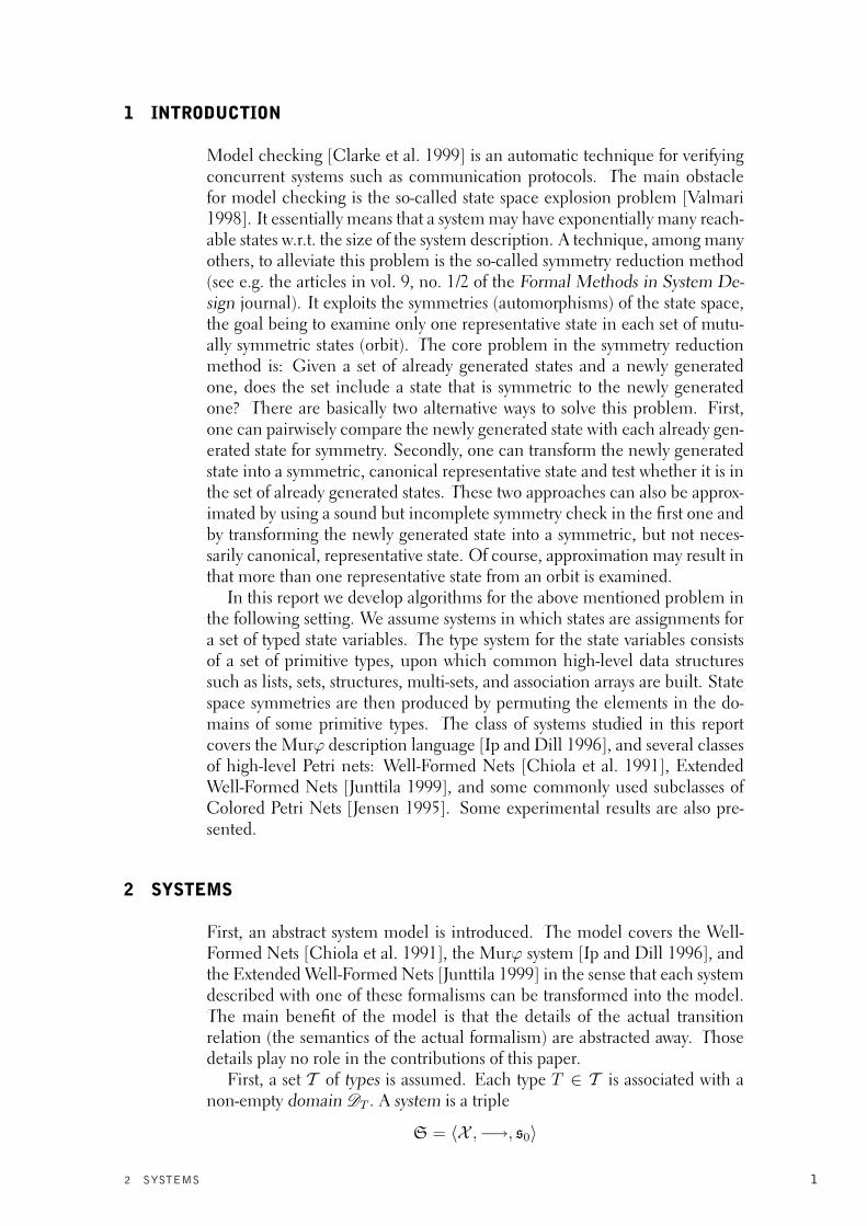
Example 3.3 Continuing Examples 2.1 and 3.1, consider the initial state

s0 = {U 7→ 〈ta, s0〉+〈tb, s3〉, V 7→ s1 + s4}.

The self-symmetry group Stab(Θ, s0) has two members:

θ1 =(θSecs

1 = ( s0 s1 s2 s3 s4 s5s0 s1 s2 s3 s4 s5 ) , θTrains

1 =( ta tb

ta tb

))and

θ2 =(θSecs


2 =( ta tb

tb ta

)).

♣

Note that although the group of allowed domain permutations Θ can bevery large, there is no need to represent it explicitly — it is implicitly repre-sented by the knowledge of which primitive types are cyclic or unordered.However, it is not so easy to represent a subgroup of Θ, for instance the stabi-lizer group of a state. Fortunately, there are efficient data structures for rep-resentation of permutation groups, see [Butler 1991]. In order to use thosedata structures, we only have to rename the domains of permutable primitivetypes to be mutually disjoint. Now any domain permutation (group) can berepresented by a permutation (group) on the set

⋃T∈TP DT .

4 VALUE TREES AND CHARACTERISTIC GRAPHS

An element of a complex structured type can be easily illustrated by its “parsetree” that is here called a value tree. Formally, for a type T and an elementv ∈ DT , the value tree VT (T, v) is an edge weighted tree that has the nodeT ::v as its root. The children of the root node are defined as follows.

– For a primitive type T , the root node T ::v has no children.– A root node List(T )::〈v1, . . . , vn〉, has as its children the value treesVT (T, vi), 1 ≤ i ≤ n, the edge to each VT (T, vi) having weight i.

– A root node Struct(T1, . . . , Tn)::〈v1, . . . , vn〉, has as its children thevalue trees VT (Ti, vi), 1 ≤ i ≤ n, the edge to each VT (Ti, vi) havingweight i.

– A root node Set(T )::V has as its children the value trees VT (T, v) foreach v ∈ V , the edge to each such VT (T, v) having weight 1.

– A root node Multi-Set(T )::m has as its children the trees VT (T, v) foreach v ∈ DT with m(v) ≥ 1, the edge to each such VT (T, v) havingweight m(v).

– A root node AssocArray(T1, T2)::a has, for each 〈v1, v2〉 ∈ a, the fol-lowing tree as its child with the edge to it having weight 1. The childtree consists of an anonymous root node with two children: the valuetree VT (T1, v1) with the edge to it having weight 1 and the value treeVT (T2, v2) with the edge to it having weight 2.

– A root node Union(T1, . . . , Tn)::〈Ti, vi〉 has the value tree VT (Ti, vi)as its only child, the edge to it having weight 1.

8 4 VALUE TREES AND CHARACTERISTIC GRAPHS

Struct(Bool, PIDs)::〈false , pid2〉

PIDs::pid1 Bool::false PIDs::pid2

Struct(Bool, PIDs)::〈true, pid1〉

PIDs::pid3 Bool::true PIDs::pid1

AssocArray(PIDs, Struct(Bool, PIDs))::{pid1 7→ 〈false , pid2〉, pid3 7→ 〈true, pid1〉}

1 1

1 12 2

1 2 1 2

Figure 5: A value tree

Example 4.1 Fig. 5 shows the value tree for the element

{pid1 7→ 〈false, pid2〉, pid3 7→ 〈true, pid1〉}

of type AssocArray(PIDs,Struct(Bool,PIDs)), where PIDs is a primitivetype with the domain DPIDs = {pid1, pid2, pid3, pid4} and Bool is a primi-tive type with the domain DBool = {false, true}. ♣

It is straightforward to see that value trees have the following property:

Fact 4.2 If there is a path T ::v w1−→ n1w2−→ n2 · · ·nk

wk+1−→ T ′::v′ from theroot node T ::v to a leaf node T ′::v′ in a value tree VT (T, v), then for eachallowed domain permutation θ there is a path T ::θT (v)

w1−→ θ(n1)w2−→

θ(n2) · · · θ(nk)wk+1−→ T ′::θT ′(v′) from the root node T ::θT (v) to a leaf node

T ′::θT ′(v′) in the value tree VT (T, θT (v)) (where θ(ni) is an anonymousnode if ni is, and Ti::θTi(vi) if ni = Ti::vi).

Assume a state variable x of type T . The value tree of x in a state s consistsof the root node x that has the value tree VT (T, s(x)) as its only child, theedge to it having weight 1. Now the characteristic graph of a state s is a nodelabeled and edge weighted directed graph Gs obtained as follows.

1. Take the disjoint union of the value trees of each state variable x in thestate s.

2. For each primitive type T and each element v ∈ DT , merge all thenodes T ::v into one node.

3. For each permutable primitive type T , if there is no node T ::v for anelement v ∈ DT , include it into the graph.

4. For each cyclic primitive type T , add a directed edge of weight 1 fromeach node T ::v to its successor node T ::succT (v)

5. Label nodes as follows:(a) Each node T ::v for a permutable primitive type T is labeled with

T .(b) Each node T ::v for an ordered primitive type T is labeled with

T.v.(c) Each node T ::v for a non-primitive type T is labeled with T .(d) Each node x corresponding to a state variable x is labeled with

var_x.

4 VALUE TREES AND CHARACTERISTIC GRAPHS 9

Struct(Bool, PIDs)::〈false , pid2〉

PIDs::pid1 Bool::false PIDs::pid2

Struct(Bool, PIDs)::〈true, pid1〉

PIDs::pid3 Bool::truePIDs::pid4

AssocArray(PIDs, Struct(Bool, PIDs))::{pid1 7→ 〈false , pid2〉, pid3 7→ 〈true, pid1〉}

1 1

1 12 2

Bool.false Bool.true21 1

2

PIDs PIDs

Struct(Bool, PIDs) Struct(Bool, PIDs)

AssocArray(PIDs, Struct(Bool, PIDs))

x2

1

x1

Struct(PIDs, PIDs)::〈pid1, pid1〉

1

2

1

Struct(PIDs, PIDs)

PIDs PIDs

var x2 var x2

Figure 6: A characteristic graph

Example 4.3 Recall the previous example and assume that Bool is an or-dered primitive type and PIDs is an unordered primitive type. Figure 6 nowshows the characteristic graph of a state s over two state variables: (i) x1

of type Struct(PIDs,PIDs) having the value s(x1) = 〈pid1, pid1〉, and (ii)x2 of type AssocArray(PIDs,Struct(Bool,PIDs)) having the value s(x2) ={pid1 7→ 〈false, pid2〉, pid3 7→ 〈true, pid1〉}. Note especially that thereare two edges from the node Struct(PIDs,PIDs)::〈pid1, pid1〉 to the nodePIDs::pid1, and that there is an isolated node PIDs::pid4. ♣

An isomorphism from a node labeled and edge weighted directed graphto another such graph is a bijective mapping from nodes to nodes preserv-ing node labels, edges, and edge weights. Two such graphs are isomorphic ifthere is an isomorphism between them. Since isomorphisms have to preservenode labels and edge weights, it is quite straightforward to see that character-istics graphs have the following properties:

Fact 4.4 For all allowed domain permutations θ, there is an isomorphism γfrom the characteristic graph Gs of a state s to the characteristic graph Gθ(s)

of the state θ(s) such that for each permutable primitive type T and for eachelement v ∈ DT , θT (v) = v′ ⇔ γ(T ::v) = T ::v′.

Fact 4.5 If there is an isomorphism γ from the characteristic graph Gs ofa state s to the characteristic graph Gs′ of a state s′, then there is a uniqueallowed domain permutation θ mapping s to s′ such that for each permutableprimitive type T and for each v ∈ DT , γ(T ::v) = T ::v′ ⇔ θT (v) = v′.

From these two facts it follows directly that the characteristic graphs of twostates are isomorphic iff the states are symmetric. Furthermore, the self-symmetry group of a state can be easily extracted from the automorphismgroup of the characteristic graph of the state.

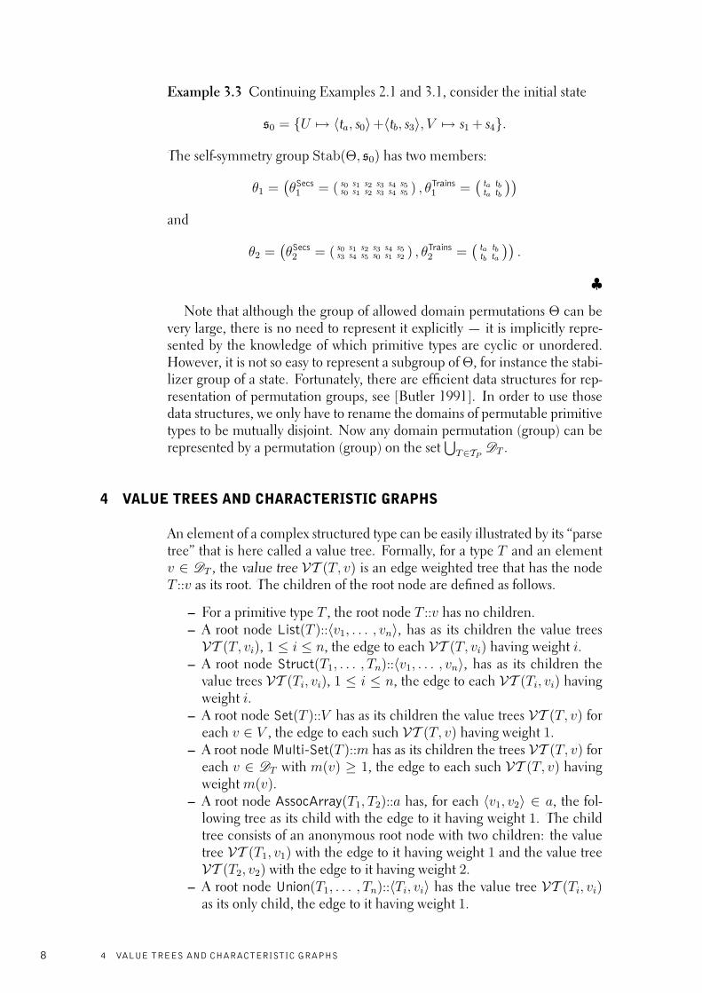
Example 4.6 Recall Examples 2.1 and 3.1. Figure 7 shows the characteris-tic graph for the state {U 7→ 〈ta, s0〉+〈tb, s3〉, V 7→ s1 + s4}. (For the sakeof simplicity, we have omitted some node names and labels that should beobvious). ♣

10 4 VALUE TREES AND CHARACTERISTIC GRAPHS

Secs::s0 Secs::s1 Secs::s2 Secs::s3 Secs::s4 Secs::s5Trains::tbTrains::ta

U V

1 1 1 1 11

1 1

1 1

2 21 1

1 1

var U var V

Figure 7: A characteristic graph

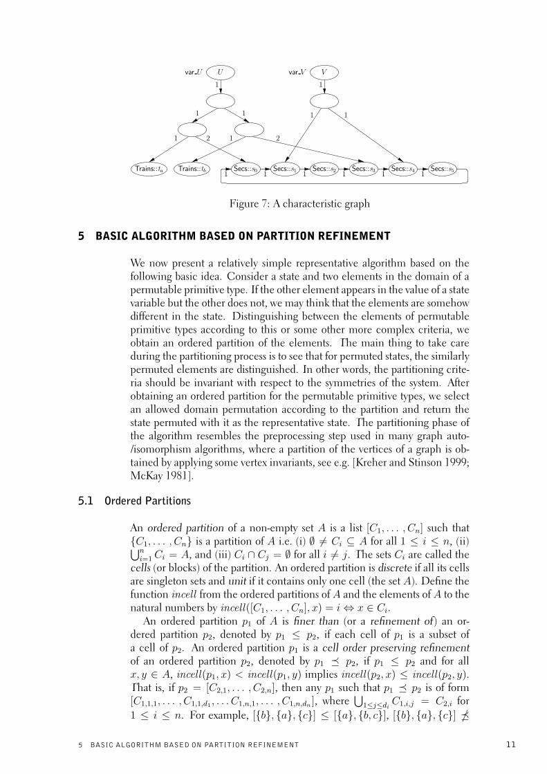
5 BASIC ALGORITHM BASED ON PARTITION REFINEMENT

We now present a relatively simple representative algorithm based on thefollowing basic idea. Consider a state and two elements in the domain of apermutable primitive type. If the other element appears in the value of a statevariable but the other does not, we may think that the elements are somehowdifferent in the state. Distinguishing between the elements of permutableprimitive types according to this or some other more complex criteria, weobtain an ordered partition of the elements. The main thing to take careduring the partitioning process is to see that for permuted states, the similarlypermuted elements are distinguished. In other words, the partitioning crite-ria should be invariant with respect to the symmetries of the system. Afterobtaining an ordered partition for the permutable primitive types, we selectan allowed domain permutation according to the partition and return thestate permuted with it as the representative state. The partitioning phase ofthe algorithm resembles the preprocessing step used in many graph auto-/isomorphism algorithms, where a partition of the vertices of a graph is ob-tained by applying some vertex invariants, see e.g. [Kreher and Stinson 1999;McKay 1981].

5.1 Ordered Partitions

An ordered partition of a non-empty set A is a list [C1, . . . , Cn] such that{C1, . . . , Cn} is a partition of A i.e. (i) ∅ 6= Ci ⊆ A for all 1 ≤ i ≤ n, (ii)⋃ni=1 Ci = A, and (iii) Ci ∩ Cj = ∅ for all i 6= j. The sets Ci are called the

cells (or blocks) of the partition. An ordered partition is discrete if all its cellsare singleton sets and unit if it contains only one cell (the set A). Define thefunction incell from the ordered partitions of A and the elements of A to thenatural numbers by incell([C1, . . . , Cn], x) = i⇔ x ∈ Ci.

An ordered partition p1 of A is finer than (or a refinement of) an or-dered partition p2, denoted by p1 ≤ p2, if each cell of p1 is a subset ofa cell of p2. An ordered partition p1 is a cell order preserving refinementof an ordered partition p2, denoted by p1 � p2, if p1 ≤ p2 and for allx, y ∈ A, incell(p1, x) < incell(p1, y) implies incell(p2, x) ≤ incell(p2, y).That is, if p2 = [C2,1, . . . , C2,n], then any p1 such that p1 � p2 is of form[C1,1,1, . . . , C1,1,d1 , . . . C1,n,1, . . . , C1,n,dn ], where

⋃1≤j≤di C1,i,j = C2,i for

1 ≤ i ≤ n. For example, [{b}, {a}, {c}] ≤ [{a}, {b, c}], [{b}, {a}, {c}] �

5 BASIC ALGORITHM BASED ON PARTITION REFINEMENT 11

[{a}, {b, c}], and [{a}, {c}, {b}] � [{a}, {b, c}]. The relation � is reflexive,transitive and antisymmetric, i.e. a partial order on the set of all ordered par-titions of A.

A permutation γ ofA acts on ordered partitions ofA by γ([C1, . . . , Cn]) =[γ(C1), . . . , γ(Cn)]. Clearly, incell(p, x) = incell(γ(p), γ(x)) for all orderedpartitions p of A and all x ∈ A. Furthermore, if γ(p1) = p2, p1 � p3, andp2 � p3, then γ(p3) = p3.

5.2 Basic Algorithm

We now present the basic representative state algorithm. The idea is that,given a state for which we wish to compute a representative,

1. we first assign the state in a symmetry respecting way a partitioning ofthe domains of the permutable primitive types,

2. then select an allowed domain permutation based on the partitioning,and

3. finally return the state permuted with the selected domain permutationas the representative.

First, we define an ordered permutable primitive type partition to be afamily p =

(pT)T∈TP

, where each pT is an ordered partition of the domainDT . The set of all ordered permutable primitive type partitions is denoted byP. The definitions for ordered partitions are naturally extended to orderedpermutable primitive type partitions. That is, p is discrete (unit) if all itsconstituent partitions are discrete (unit). Similarly, a domain permutationψ =

(ψT)T∈TP

acts on a partition p =(pT)T∈TP

by ψ(p) =(ψT (pT )

)T∈TP

and(pT1)T∈TP

�(pT2)T∈TP

if pT1 � pT2 for all T ∈ TP . As we will dealexclusively with ordered partitions, we usually omit the prefix “ordered” andsimply speak of partitions. For convenience, we may also omit the prefix“permutable primitive type” whenever no confusion can arise.

Given a state s, we associate it with a partition by using a function thatrespects the group of allowed domain permutations (i.e. symmetries of thesystem).

Definition 5.1 (Invariant Partition Generators) A function G : S → P

that maps each state to a permutable primitive type partition is an invariantpartition generator if

G(θ(s)) = θ(G(s))

holds for all allowed domain permutations θ ∈ Θ.

That is, for permuted states the partition assigned by G should be similarlypermuted. We will develop a way to produce such functions in Sec. 5.3.

Next, we select an allowed domain permutation according to the partitionproduced by an (fixed) invariant partition generator. The set of allowed do-main permutations from which we have to select is given by the followingcompatibility definition.

Definition 5.2 (Compatibility) An allowed domain permutation(θT)T∈TP

is compatible with a partition(pT)T∈TP

if

12 5 BASIC ALGORITHM BASED ON PARTITION REFINEMENT

– For each cyclic primitive type T with DT = {v1, . . . , vn} and pT =[CT

1 , . . . , CTm], θT is such that it maps an element v ∈ CT

1 to v1.– For each unordered primitive type T with DT = {v1, . . . , vn} and

pT = [CT1 , . . . , C

Tm], θT must fulfill the following: if incell(pT , vi) <

incell(pT , vj), then for the permuted elements vi′ = θT (vi) and vj′ =θT (vj) it holds that i′ < j′. That is, the n1 elements in the first cell CT

1

are mapped to v1, . . . , vn1 , the n2 elements in the second cell CT2 are

mapped to vn1+1, . . . , vn1+n2 , and so on.

Obviously, for each partition there is at least one allowed domain permuta-tion compatible with it.

To sum up, assuming an arbitrary but fixed invariant partition generator G,the procedure for generating (not necessarily canonical) representative statesis described in Alg. 1.

Algorithm 1 Representative algorithm 1Input: A state s

Output: A representative state that is symmetric to s

Require: An invariant partition generator G1: Compute the partition p = G(s)2: Choose any allowed domain permutation θ that is compatible with p

3: Return θ(s) as the representative state

The following lemma and corollary show that this algorithm preserves thepossibility for perfect reduction in the sense that, for all symmetric states, itis possible to choose the same representative state. That is, there is nothinginherent in the algorithm that would force the set of representative states fora set of mutually symmetric states to contain more than one state. Of course,choosing the right allowed domain permutations in line 2 of Alg. 1 may re-quire an exponential amount of work or very good luck, but nevertheless it ispossible to do so.

Lemma 5.3 Let θ be an allowed domain permutation compatible with apartition p. Then for each allowed domain permutation θ it holds that theallowed domain permutation θ ∗ θ−1 is compatible with the partition θ(p).

Corollary 5.4 Assume an invariant partition generator G, and take two sym-metric states, s1 and s2. Let θ1 be an allowed domain permutation compat-ible with the partition G(s1). Then there is an allowed domain permutationθ2 compatible with the partition G(s2) such that θ1(s1) = θ2(s2).

Example 5.5 Consider the state s = {U 7→ 〈ta, s1〉+〈tb, s3〉, V 7→ s4 + s5}for the railroad system net in Fig. 1 (recall Ex. 2.1 and Ex. 3.1). Assume aninvariant partition generator G that produces the partition

G(s) =(pSecs

s,4 = [{s0, s2}, {s4, s5}, {s1, s3}], pTrainss,4 = [{ta, tb}]

).

for s. Having the fixed ordering s0 < s1 < · · · < s5 between the railroadsections and ta < tb between the train identities, the four possible domain


permutations compatible with the partition are

θ1 =(θSecs


1 =( ta tb

ta tb

)),

θ2 =(θSecs


2 =( ta tb

tb ta

)),

θ3 =(θSecs


3 =( ta tb

ta tb

)), and

θ4 =(θSecs


4 =( ta tb

tb ta

)).

The corresponding possible representative states for s are:

θ1(s) = {U 7→ 〈ta, s1〉+〈tb, s3〉, V 7→ s4 + s5} = s,

θ2(s) = {U 7→ 〈ta, s3〉+〈tb, s1〉, V 7→ s4 + s5},θ3(s) = {U 7→ 〈ta, s5〉+〈tb, s1〉, V 7→ s2 + s3}, andθ4(s) = {U 7→ 〈ta, s1〉+〈tb, s5〉, V 7→ s2 + s3}.

Now consider the state s′ = {U 7→ 〈ta, s0〉+〈tb, s4〉, V 7→ s1 + s2} ob-tained from s by rotating the railroad sections 3 steps and swapping the trainidentities, i.e. by applying

θ =(θSecs = ( s0 s1 s2 s3 s4 s5


tb ta

)).

Since s′ = θ(s), the invariant partition generator G must assign the partitionθ(G(s)) to s′, i.e.

G(s′) = θ(G(s)) =(pSecs

s′,4 = [{s3, s5}, {s1, s2}, {s0, s4}], pTrainss′,4 = [{ta, tb}]

).

The four possible domain permutations compatible with the partition are

θ1′ =(θSecs

1′ = ( s0 s1 s2 s3 s4 s5s3 s4 s5 s0 s1 s2 ) , θTrains

1′ =( ta tb

ta tb

))= θ2 ∗ θ−1,

θ2′ =(θSecs


2′ =( ta tb

tb ta

))= θ1 ∗ θ−1,

θ3′ =(θSecs


3′ =( ta tb

ta tb

))= θ4 ∗ θ−1, and

θ4′ =(θSecs


4′ =( ta tb

tb ta

))= θ3 ∗ θ−1.

The corresponding possible representative states for s′ are:

θ1′(s′) = {U 7→ 〈ta, s3〉+〈tb, s1〉, V 7→ s4 + s5} = θ2(s),

θ2′(s′) = {U 7→ 〈ta, s1〉+〈tb, s3〉, V 7→ s4 + s5} = θ1(s),

θ3′(s′) = {U 7→ 〈ta, s1〉+〈tb, s5〉, V 7→ s2 + s3} = θ4(s), and

θ4′(s′) = {U 7→ 〈ta, s5〉+〈tb, s1〉, V 7→ s2 + s3} = θ3(s).

Thus the sets of possible representative states for s and s′ are the same. Thiswas expected because of Lemma 5.3, Corollary 5.4, and the fact that s and s′

are symmetric. ♣

Producing Canonical Representative StatesAssuming that the set S of states is totally ordered, algorithm Alg. 1 can beextended to produce canonical representative states. For a state s, simplycompute the partition G(s) and then check all the allowed domain permuta-tions θ that are compatible with G(s) and return the smallest state θ(s) foundas the representative state. By Cor. 5.4, this procedure produces canonicalrepresentative states.


5.3 Partition Refiners and Invariants

We now focus on building invariant partition generators. First, we introducepartition refiners. They are functions that, given a state and a partition, returna cell order preserving refinement of the partition in a symmetry respectingway.

Definition 5.6 (Partition Refiners) A partition refiner is a functionR : S ×P→ P such that for all states s ∈ S and for all partitions p ∈ P it holds that(i) R(s, p) � p and (ii) θ(R(s, p)) = R(θ(s), θ(p)) for all allowed domainpermutations θ.

Partition refiners can be composed:

Lemma 5.7 The composition R2 ?R1 of two partition refiners R1 and R2,defined by (R2 ?R1)(s, p) = R2(s,R1(s, p)), is a partition refiner.

This implies that any finite sequenceRn?Rn−1?· · ·?R1 of partition refiners,read byRn?(Rn−1?(· · · (R2?R1))) orRn(s,Rn−1(s, · · · (s,R1(s, p)) . . . )),is also a partition refiner. That is, we first refine the argument partition withthe first refiner, then refine the resulting partition with the second refiner,and so on. When a partition refiner is applied to the unit partition, the resultis an invariant partition generator.

Theorem 5.8 For a partition refiner R, the function GR(s) = R(s, p0),where p0 =

(pT0 = [DT ]

)T∈TP

is the unit partition, is an invariant partitiongenerator.

Now the task of building invariant partition generators is reduced to build-ing partition refiners. This task is accomplished by using invariants. Aninvariant is a function that tries to distinguish between the elements of apermutable primitive type under a given state and partition. It must distin-guish the elements in a way that respects the allowed domain permutations,i.e. under a permuted state and partition, the invariant should distinguish thesimilarly permuted elements. Formally, we define the following:

Definition 5.9 (Invariants) An invariant for a permutable primitive type Tis a function I from the domain DT × S × P such that for all elementsv ∈ DT , for all states s ∈ S, for all partitions p ∈ P, and for all alloweddomain permutations θ ∈ Θ, it holds that

I(v, s, p) = I(θT (v), θ(s), θ(p)).

The codomain of I is assumed to be a set with a total order <.

We say that an invariant I is partition independent if it does not depend onthe partition argument, otherwise it is partition dependent. Invariants canalso be defined for types instead of states:

Definition 5.10 (Type Invariants) A type invariant for a permutable primi-tive type T in a type T ′ is a function I from the domain DT ×DT ′ ×P such


that for all elements v ∈ DT , for all elements v′ ∈ DT ′ , for all partitionsp ∈ P, and for all allowed domain permutations θ ∈ Θ, it holds that

I(v, v′, p) = I(θT (v), θT′(v′), θ(p)).

Again, the codomain of I is assumed to be a set with a total order <.

Type invariants can be interpreted as invariants:

Lemma 5.11 If I is a type invariant for a permutable primitive type T in atype T ′ and x is a state variable of type T ′, then Ix(v, s, p) = I(v, s(x), p) isan invariant for T .

Example 5.12 Define for each primitive type T and for each type T ′ thefunction ]T ′T : DT ×DT ′ → N∪ {∞}, read “the element v of type T appears]T′

T (v, v′) times in the element v′ of type T ′”, by the following rules:

1. If T ′ is primitive type, then ]T ′T (v, v′) = 1 if T = T ′ and v = v′, and 0otherwise.

2. ]List(T ′)T (v, 〈v′1, . . . , v′n〉) =

∑1≤i≤n ]

T ′T (v, v′i)

3. ]Struct(T ′1,... ,T′n)

T (v, 〈v′1, . . . , v′n〉) =∑

1≤i≤n ]T ′iT (v, v′i)

4. ]Set(T ′)T (v, V ′) =

∑v′∈V ′ ]

T ′T (v, v′)

5. ]Multi-Set(T ′)T (v,m) =

∑v′∈DT ′

m(v′) · ]T ′T (v, v′)

6. ]AssocArray(T ′1,T′2)

T (v, a) =∑〈v′1,v′2〉∈a

(]T ′1T (v, v′1) + ]

T ′2T (v, v′2))

7. ]Union(T ′1,... ,T′n)

T (v, 〈T ′i , v′〉) = ]T ′iT (v, v′)

It is easy to see that ]T ′T (v, v′) = ]T′

T (θT (v), θT′(v′)) for all allowed domain

permutations θ. Now the function I]T in T ′(v, v′, p) = ]T

′T (v, v′) is a partition

independent type invariant for T in T ′. If x is a state variable of type T ′, thenthe corresponding invariant is I]T in x(v, s, p) = I]T in T ′(v, s(x), p), i.e. thenumber of times v appears in the value of x in the state s. ♣

We will introduce more invariants later, including some partition depen-dent ones, too. Given an invariant for a permutable primitive type T and apartition p, we may refine the partition according to the invariant by splittingthe cells of the partition for T so that each new cell contains all the elementsin the original cell that are assigned to the same value by the invariant.

Definition 5.13 Given an invariant I for a permutable primitive type T , de-fine the functionRI : S ×P→ P byRI(s, p) = pref, where

1. for any permutable primitive type T ′ 6= T , pT′

ref = pT′ , and

2. the partition pTref is the one such that for all v, v′ ∈ DT ,(a) incell(pTref, v) = incell(pTref, v

′) iff incell(pT , v) = incell(pT , v′)and I(v, s, p) = I(v′, s, p), and

(b) if incell(pTref, v) < incell(pTref, v′), then either

i. incell(pT , v) < incell(pT , v′), orii. incell(pT , v) = incell(pT , v′) and I(v, s, p) < I(v′, s, p).

Lemma 5.14 The functionRI is a partition refiner.


When the partition refiner RI is applied to a partition p in a state s,i.e. partition p is replaced by RI(s, p), we say that p is refined according toI . Given a sequence I1.I2. . . . .In of invariants (for arbitrary primitive types),we say that a partition p is refined according to the sequence to mean thatthe partition refiner sequenceRIn ?RIn−1 ? · · · ?RI1 is applied to it.

To sum up, we obtain an invariant partition generator by (i) defining asequence I1.I2. . . . .In of invariants, and (ii) refining the unit partition ac-cording to the sequence (by Lemma 5.14 and Thm. 5.8).

Example 5.15 Consider the state s = {U 7→ 〈ta, s1〉+〈tb, s3〉, V 7→ s4 + s5}for the railroad system net in Fig. 1 (cf Ex. 5.5). Initially, the partition is theunit partition

ps,0 =(pSecs

s,0 = [{s0, s1, s2, s3, s4, s5}], pTrainss,0 = [{ta, tb}]

).

We now apply the invariant sequence I]Trains in U .I]Trains in V .I]Secs in U .I]Secs in V

to the partition (recall Ex. 5.12). Refining the partition for Trains accordingto the invariant I]Trains in U leads to

ps,1 =(pSecs


),

i.e. does not change anything since both ta and tb appear once in the valueof U . Similarly, refining the partition for Trains according to the invariantI]Trains in V changes nothing. Refining the partition for Secs according to theinvariant I]Secs in U leads to

ps,3 =(pSecs

s,3 = [{s0, s2, s4, s5}, {s1, s3}], pTrainss,3 = [{ta, tb}]

),

distinguishing the railroad sections s1 and s3 from the others because theyappear once in the value of U while the others do not. Further refiningaccording to the invariant I]Secs in V gives us

ps,4 =(pSecs


).

Applying the same sequence of invariants to the state s′ = θ(s) = {U 7→〈ta, s0〉+〈tb, s4〉, V 7→ s1 + s2}, where θ is as defined in Ex. 5.5, gives thepartition

ps′,4 = θ(ps,4) =(pSecs


).

♣

5.4 Some Useful Invariants

A Successor Based Invariant for Cyclic Primitive TypesWe are now ready to introduce our first partition dependent invariant. Usingthis invariant, it is possible to exploit the partition produced so far to obtainfurther partition refinement. For a cyclic primitive type T , consider the func-tion

IT,succ(v, s, p) = incell(pT , succT (v))

i.e. the function that returns the cell number of the successor element ofthe element v in the partition p. That is, IT,succ distinguishes between twoelements if their successors are already distinguished in the current partitionp.


Lemma 5.16 The function IT,succ is an invariant.

Therefore, if we have refined the initial partition according to an invariantsequence, we may further refine the resulting partition by using the invariantIT,succ. The resulting partition may again be further refined by the sameinvariant until no refinement happens i.e. we reach a fixed point (in otherwords, the sequence of length |DT | of invariant IT,succ is applied). Note that,while IT,succ is partition dependent, it does not depend on the state argumenti.e. is state independent.

Example 5.17 Reconsider the state

s = {U 7→ 〈ta, s1〉+〈tb, s3〉, V 7→ s4 + s5}

and the partition

ps,4 =(pSecs


)for it given in Ex. 5.15. Evaluating the invariant ISecs,succ in the partition gives

ISecs,succ(s0, s, ps,4) = 3, ISecs,succ(s1, s, ps,4) = 1,ISecs,succ(s2, s, ps,4) = 3, ISecs,succ(s3, s, ps,4) = 2,ISecs,succ(s4, s, ps,4) = 2, and ISecs,succ(s5, s, ps,4) = 1.

Refining according to this results in the partition

ps,5 =(pSecs

s,5 = [{s0, s2}, {s5}, {s4}, {s1}, {s3}], pTrainss,5 = [{ta, tb}]

).

Further evaluating the invariant ISecs,succ in this partition gives

ISecs,succ(s0, s, ps,5) = 4, ISecs,succ(s1, s, ps,5) = 1,ISecs,succ(s2, s, ps,5) = 5, ISecs,succ(s3, s, ps,5) = 3,ISecs,succ(s4, s, ps,5) = 2, and ISecs,succ(s5, s, ps,5) = 1.

Refining according to this results in the partition

ps,6 =(pSecs

s,6 = [{s0}, {s2}, {s5}, {s4}, {s1}, {s3}], pTrainss,6 = [{ta, tb}]

).

Now there are only two domain permutations compatible with the partition:

θ1 =(θSecs


1 =( ta tb

ta tb

)), and

θ2 =(θSecs


2 =( ta tb

tb ta

)).

The corresponding possible representative states for s are:

θ1(s) = {U 7→ 〈ta, s1〉+〈tb, s3〉, V 7→ s4 + s5} = s, andθ2(s) = {U 7→ 〈ta, s3〉+〈tb, s1〉, V 7→ s4 + s5}.

Applying the same successor invariants to the state

s′ = {U 7→ 〈ta, s0〉+〈tb, s4〉, V 7→ s1 + s2}

in the partition

ps′,4 =(pSecs


)18 5 BASIC ALGORITHM BASED ON PARTITION REFINEMENT

results in

ps′,6 =(pSecs

s′,6 = [{s3}, {s5}, {s2}, {s1}, {s4}, {s0}], pTrainss′,6 = [{ta, tb}]

).

Now the two domain permutations compatible with the partition are:

θ1′ =(θSecs


1′ =( ta tb

ta tb

)), and

θ2′ =(θSecs


2′ =( ta tb

tb ta

)).

The corresponding possible representative states for s′ are:

θ1′(s′) = {U 7→ 〈ta, s3〉+〈tb, s1〉, V 7→ s4 + s5} = θ2(s), and

θ2′(s′) = {U 7→ 〈ta, s1〉+〈tb, s3〉, V 7→ s4 + s5} = θ1(s) = s.

♣

Ordered Structured TypesConsider a structured type T ′ composed only of primitive types, lists, struc-tures and unions. Now the value tree (recall Sec. 4) for any v′ ∈ DT ′ isordered in the sense that the children of each node can be totally ordered bythe arc labelings. Therefore, it is possible to uniquely number the nodes inthe value tree, for instance in a depth-first manner. Now each element v ofa primitive subtype T of T ′ that appears in the element v′ can be associatedwith a unique number, e.g. the smallest number of those nodes of form T ::vin the tree. The elements of T ′ not appearing in v′ can be associated withthe number 0. For instance, consider the value tree shown in Fig. 8 for theelement l = 〈〈v3, 3, u1〉, 〈v3, 2, u3〉〉 of type List(Struct(T1, Int, T2)), whereT1 is an unordered primitive type with DT1 = {v1, v2, v3, v4} and T2 is acyclic primitive type with DT2 = {u1, u2, u3, u4}. The depth-first numberingof nodes is shown in boldface font in the figure. Thus the elements of T1 areassociated with integers by the mapping {v1 7→ 0, v2 7→ 0, v3 7→ 1, v4 7→ 0}and those of T2 by {u1 7→ 3, u2 7→ 0, u3 7→ 7, u4 7→ 0}. Define the func-tion Idfs-numbering of T in T ′ : DT × DT ′ ×P → N to be the mapping describedabove. It should be obvious that it is a partition independent type invariantwith the following property: if two elements, v1 and v2, of type T appear inthe element v′, then I(v1, v

′, p) 6= I(v2, v′, p). Therefore, refining a partition

according to such an invariant leads to a partition in which all the elementsappearing in the element v′ are in their own cells. For cyclic primitive types,the resulting partition should be further refined by using the successor basedinvariant described earlier.

The above procedure does not work for structured types composed of sets,multi-sets or association arrays. This is because the value tree is not orderedin the above sense and therefore we cannot assign the nodes in it a uniquenumbering. However, this restriction can be circumvented in some spe-cial cases. For instance, consider an association array where the domainof the first type (the type whose elements are associated with elements ofthe second type) is not permuted by allowed domain permutations, e.g. atype AssocArray(Int[1-3],Struct(T1, Int)), where Int[1-3] with the domainDInt[1-3] = {1, 2, 3} is an ordered primitive type. This type corresponds to anormal array of size 3 (with possibly undefined elements), and the elements


Int::3T1::v3 T2::u1 Int::2 T2::u3

12

32

31

21

4 8

9

T1::v3

1 2 3 5 6 7

Figure 8: An ordered value tree

Int[1-3]::1

1 2

Int[1-3]::3

1 2

T1::v3 Int::7 T1::v2 Int::1

1 2 21

T1::v3 Int::7 T1::v2 Int::1

1 2 21

1 3

Figure 9: Mapping an unordered value tree into an ordered one

in it are totally ordered. In this kind of case the value tree can be modifiedto be ordered, as shown in Fig. 9 for an element {1 7→ 〈v3, 7〉, 3 7→ 〈v2, 1〉},and the above procedure for producing type invariants can be applied.

Although state variables of the “easy” structured types described above arecommon in Murϕ descriptions, in high-level Petri nets the state variables areof multi-set types which are not handled by the above procedure. Yet theabove procedure can be applied to multi-sets over the “easy” structured typesin some important special cases: if a multi-set contains only one element orall the elements in the multi-set have different multiplicities, then the valuetree becomes ordered and the above procedure works fine. The same appliesto set types in the case a set contains only one element.

There is an important special case that often occurs in high-level Petrinets: a state variable of type Multi-Set(T ), where T is a permutable prim-itive type. Define the partition independent invariant Imultiplicity : DT ×DMulti-Set(T ) ×P → N by Imultiplicity(v,m, p) = m(v). In the case T is an un-ordered primitive type, Imultiplicity has the property that if a partition is refinedaccording to this invariant, resulting in a partition p1, then θMulti-Set(T )

2 (m) =

θMulti-Set(T )3 (m) for all allowed domain permutations θ2 and θ3 that are com-

patible with partitions p2 � p1 and p3 � p1, respectively. Thus Imultiplicity insome sense canonizes the multi-set value m.

Hash-Like InvariantsThe invariants we have been using so far have been quite simple. We couldintroduce more complicated special invariants, but there are too many ofthem to cover all imaginable cases. For instance, assuming a state variablex of type Multi-Set(Struct(Int, T )), where Int with DInt = {0, 1, 2, . . . } isan ordered primitive type, the function IT,x,〈3,v〉 for the type T defined byIT,x,〈3,v〉(v, s, p) = s(x)(〈3, v〉), i.e. the number of 〈3, v〉-elements in thevalue of x in the state s, is an invariant. The more complicated the types


of the state variables get, the more complicated the possible invariants get,too. We now show how to calculate a general purpose invariant that dependson the structure of a state in a degree larger than the earlier ones. It is alsopartition dependent. Moreover, calculating the invariant is relatively easy: itresembles the way one would compute a hash value for a structured object.

For each primitive type T , we define a function

gT (v, T ′, v′, p)

over four arguments: the first argument is an element v in the domain of thetype T , the second argument is a type T ′, the third argument is an elementv′ in the domain of the type T ′, and the last argument is a partition. The firstargument v is the element for which we compute the “hash value”, while thesecond and third arguments describe the object in which we perform thiscomputation. The fourth argument gives the current partition. The functiongT is defined recursively top-down on the structure of the second argumenttype T ′: the value depends on the values of the subtypes of T ′. In the leaves,when T ′ is a primitive type, the function has a value depending on (i) therelationship between the types T and T ′, (ii) the relationship between thevalues as the first and third argument, and (iii) the partition into which thethird argument belongs.

Firstly, we assume an associative and commutative binary operation ⊕ onZ. Furthermore, for a type T , hT : Z → Z and hT,n : Zn → Z are assumedto be arbitrary functions unless otherwise stated. The inductive definition ofthe function gT now is:

1. For an ordered primitive type T ′, gT (v, T ′, v′, p) = hT ′(v′), where hT ′

is a function from DT ′ to Z.2. For a cyclic primitive type T ′ with DT ′ = {v1, . . . , vn},

gT (v, T ′, v′, p) ={hT ′(incell(pT

′, v′)) if T 6= T ′

hT ′,2(k, incell(pT′, v′)) if T = T ′ and v′ is the k-successor of v.

3. For an unordered primitive type T ′,

gT (v, T ′, v′, p) =

{hT ′,2(incell(pT

′, v′), 0) if T 6= T ′ or T = T ′ ∧ v 6= v′

hT ′,2(incell(pT′, v′), 1) if T = T ′ and v = v′.

4. For a list type T ′ = List(T1),

gT (v, T ′, 〈v1, . . . , vn〉, p) = hT ′,n(gT (v, T1, v1, p), . . . , gT (v, T1, vn, p)).

5. For a structure type T ′ = Struct(T1, . . . , Tn),

gT (v, T ′, 〈v1, . . . , vn〉, p) = hT ′,n(gT (v, T1, v1, p), . . . , gT (v, Tn, vn, p)).

6. For a set type T ′ = Set(T1),

gT (v, T ′, v′, p) = hT ′

(⊕v′′∈v′

gT (v, T1, v′′, p)

).


7. For a multi-set type T ′ = Multi-Set(T1),

gT (v, T ′, v′, p) = hT ′

⊕v′′∈DT1

,v′(v′′)≥1

hT ′,2(v′(v′′), gT (v, T1, v′′, p))

.

8. For an association array type T ′ = AssocArray(T1, T2),

gT (v, T ′, v′, p) = hT ′

⊕〈v1,v2〉∈v′

hT ′,2(gT (v, T1, v1, p), gT (v, T2, v2, p))

.

9. For an union type T ′ = Union(T1, . . . , Tn),

gT (v, T ′, 〈Ti, v′〉, p) = hT ′(gT (v, Ti, v′, p)).

Lemma 5.18 If θ =(θT)T∈T is an allowed domain permutation, then

gT (v, T ′, v′, p) = gT (θT (v), T ′, θT′(v′), θ(p)).

Corollary 5.19 For a permutable primitive type T and for a type T ′,

IT,hash in T ′(v, v′, p) = gT (v, T ′, v′, p)

is a type invariant. Similarly, if x is a state variable of type T ′, then

IT,hash in x(v, s, p) = gT (v, T ′, s(x), p)

is an invariant.

Example 5.20 Consider again the state s = {U 7→ 〈ta, s1〉+〈tb, s3〉, V 7→s4 + s5} for the railroad system net in Fig. 1, recall Examples 5.5, 5.15 and5.17. Let ⊕ be the integer addition operation, and let

hTrains,2(1, 0) = 374, hTrains,2(2, 0) = 1374,hTrains,2(1, 1) = 242 · 374, hTrains,2(2, 1) = 242 · 1374,hSecs,2(k, 1) = (k + 1) · 837, hSecs,2(k, 2) = (k + 1) · 274,hSecs,2(k, 3) = (k + 1) · 97, hSecs,2(k, 4) = (k + 1) · 4732,hSecs,2(k, 5) = (k + 1) · 194, hSecs,2(k, 6) = (k + 1) · 958,hMulti-Set(Struct(Trains,Secs)(x) = x, hMulti-Set(Struct(Trains,Secs)),2(x, y) = x · y,hStruct(Trains,Secs),2(x, y) = x · by

2c.

Initially, the partition is

ps,0 =(pSecs


).

When we evaluate the invariant ISecs,hash in U in the partition, we get

ISecs,hash in U (s0, s, ps,0) =gSecs(s0,Multi-Set(Struct(Trains,Secs)), 〈ta, s1〉+〈tb, s3〉, ps,0) =

1 · gSecs(s0,Struct(Trains,Secs), 〈ta, s1〉, ps,0)+1 · gSecs(s0,Struct(Trains,Secs), 〈tb, s3〉, ps,0) =

1 · (gSecs(s0,Trains, ta, ps,0) · bgSecs(s0,Secs, s1, ps,0)/2c)+1 · (gSecs(s0,Trains, tb, ps,0) · bgSecs(s0,Secs, s3, ps,0)/2c) =

1 · (hTrains(1, 0) · bhSecs,2(1, 1)/2c) + 1 · (hTrains(1, 0) · bhSecs,2(3, 1)/2c) =1 · (374 · b(2 · 837)/2c) + 1 · (374 · b(4 · 837)/2c) =

1 · (374 · 837) + 1 · (374 · 1674) =939114,


and

ISecs,hash in U(s1, s, ps,0) = 625702,



ISecs,hash in U(s4, s, ps,0) = 1565190, andISecs,hash in U(s5, s, ps,0) = 1251778.

Now the partition is refined into

ps,1 =(pSecs

s,1 = [{s1}, {s3}, {s0}, {s5}, {s2}, {s4}], pTrainss,1 = [{ta, tb}]

).

Evaluating ISecs,hash in V in this partition yields no further information sincethe partition for Secs is already discrete. Evaluating ITrains,hash in U in the parti-tion gives ITrains,hash in U(ta, s, ps,1) = 37883582 and ITrains,hash in U(tb, s, ps,1) =12555928, refining the partition into

ps,2 =(pSecs

s,2 = [{s1}, {s3}, {s0}, {s5}, {s2}, {s4}], pTrainss,2 = [{tb}, {ta}]

).

Now there is only one allowed domain permutation compatible with ps,2,namely

θ =(θSecs = ( s0 s1 s2 s3 s4 s5


tb ta

)),

and the corresponding representative state is

θ(s) = {U 7→ 〈ta, s2〉+〈tb, s0〉, V 7→ s3 + s4}.

♣

Note that the h-functions defined in the above example are not probably veryoptimal since they are quite similar. Although they suffice for demonstra-tive purposes, in a real implementation some bit twisting operations shouldbe applied instead in order to reduce the possibility of value collision. Themain thing to take care of is that the operation ⊕ is commutative and asso-ciative. The h-functions may, for instance, employ pseudo-random numbersto obtain relative independence from each other.

5.5 Limitations of Invariant Partition Generators

We now study some fundamental, inherent limitations involved in the useof invariant partition generators. Directly from the definition of invariantpartition generators we observe the following. Let s and s′ be two symmetricstates and let G be an invariant partition generator. If θ is an allowed domainpermutation mapping s to s′, then θmaps the cells in the partition G(s) to thecorresponding cells in G(s′) since G(θ(s)) = θ(G(s)) ⇒ G(s′) = θ(G(s)).From this fact we are able to obtain a lower limit for the sizes of cells inpartitions produced by any invariant partition generator.

Fact 5.21 Let θ =(θT)T∈TP

be a self-symmetry of a state s, i.e. θ(s) = s

or, equivalently, θ ∈ Stab(Θ, s). Then G(θ(s)) = θ(G(s)) implies G(s) =θ(G(s)) for any invariant partition generator G. Thus each self-symmetry of s

respects the cells in G(s), meaning that if v ∈ DT belongs to the cell CTi in

the partition G(s), then θT (v) belongs to the cell CTi , too.


Optimal invariant partition generator functions, i.e. functions that pro-duce minimal partitions whose cells are as small as possible, are probablynot, in general, computable in polynomial time. For if we could always com-pute such functions efficiently, we would know by the fact above whether thegroup Stab(Θ, s) is non-trivial (has other elements besides the identity): ifa partition has a cell with more than one element for some primitive type,then Stab(Θ, s) is non-trivial. Combined with the construction in the proofof Theorem 3.4 in [Ip 1996], the non-triviality of Stab(Θ, s) would revealus that a graph has non-trivial automorphisms. For this task we know nopolynomial-time algorithms.

6 IMPROVEMENTS BASED ON SEARCH TREES

Recall the Algorithm 1 for producing representative states. Assuming a fixedinvariant partition generator G, given a state s, we produce the partition G(s)and take arbitrarily an allowed domain permutation θ that is compatible withit and return θ(s) as the representative. In the case the partition G(s) has anon-singleton cell for a permutable primitive type, there may be many com-patible allowed domain permutations and thus, potentially but not necessar-ily, many possible representative states for s. Especially, when G(s) has anon-singleton cell of size n for an unordered primitive type, the choice ofwhich element will be the “first” one does not affect in any way the n − 1choices we must make for the rest of the elements. Nor does it affect thechoices that have to be made for other non-singleton cells. We now presentan improvement that can reduce the set of possible representative states. Inthis approach the choices may affect or eliminate the choices yet to be taken.

First, we assume a fixed invariant partition generator G and a fixed parti-tion refinerR.

Definition 6.1 (Search Trees) The search tree of a state s and a partitionp =

(pT)T∈TP

is a tree T (s, p) defined by the following inductive rules.

1. If each partition pT in p is discrete, then the tree T (s, p) is the singleleaf node p.

2. Otherwise, let pT = [CT1 , . . . , C

Tn ] be the first non-discrete partition

in p (according to some fixed ordering between the permutable primi-tive types). Let CT

i = {vi,1, vi,2, . . . } be the first non-singleton cell inpT . The tree T (s, p) then consists of the root node p which has as itschildren the trees T (s,R(s, pj)), where for each 1 ≤ j ≤

∣∣CTi

∣∣ thepartition pj is the same as p except that the partition for T is

pTj = [CT1 , . . . , C

Ti−1, {vi,j}, CT

i \ {vi,j}, CTi+1, . . . ].

In other words, for each element in the first non-discrete cell CTi , we

split the cell in two parts by distinguishing the element into its own celland refine the resulting partition with the refinement invariants. Thechild T (s,R(s, pj)) above is called the vi,j -child of the node p and theedge from p to it is labeled with T.vi,j . We use p

T.v−→ p′ to denote thatp′ is a v-child of p.

24 6 IMPROVEMENTS BASED ON SEARCH TREES

The search tree T (s) of a state s is the search tree T (s,G(s)).

We now modify our representative algorithm Alg. 1 as follows. Given astate s, we travel along one, arbitrary path in the search tree T (s) until a leafnode (discrete partition) p is encountered, take the unique allowed domainpermutation θ that is compatible with p and return θ(s) as the representative.The resulting algorithm is shown in Alg. 2.


Output: A representative state that is symmetric to s

1: Build the partition p = G(s)2: Choose any path in the search tree T (s, p) ending in a discrete partition

p′

3: Let θ be the unique allowed domain permutation compatible with p′

4: Return θ(s) as the representative state

Example 6.2 Consider the state s = {U 7→ 〈ta, s0〉+〈tb, s3〉, V 7→ s1 + s4}for the railroad system net in Fig. 1. Refining the initial partition with theinvariant sequence I]Trains in U .I]Trains in V .I]Secs in U .I]Secs in V (i.e. applying theinvariant partition generator) gives us the partition

p =(pSecs = [{s2, s5}, {s1, s4}, {s0, s3}], pTrains = [{ta, tb}]

).

This partition is the best one can get by using any invariant partition gen-erator function in the sense that the elements in any cell in it cannot bedistinguished by any such function. This is because the allowed domain per-mutation

θ =(θSecs = ( s0 s1 s2 s3 s4 s5


tb ta

))is a self-symmetry of s (recall Fact 5.21). Assuming a fixed ordering s0 < s1 <· · · < s5 between the railroad sections and ta < tb between the train iden-tities, the four possible domain permutations compatible with the partitionare

θ1 =(θSecs


1 =( ta tb

ta tb

)),

θ2 =(θSecs


2 =( ta tb

tb ta

)),

θ3 =(θSecs


3 =( ta tb

ta tb

)), and

θ4 =(θSecs


4 =( ta tb

tb ta

)).

The corresponding two possible representative states for s are:

θ1(s) = θ4(s) = {U 7→ 〈ta, s4〉+〈tb, s1〉, V 7→ s2 + s5} andθ2(s) = θ3(s) = {U 7→ 〈ta, s1〉+〈tb, s4〉, V 7→ s2 + s5}.

Assume the partition refiner R that is induced by the invariant sequencethat first contains 6 ISecs,succ invariants and after those enough hash-like in-variants described in Sec. 5.4. The search tree T (s, p) has p as the root node.The cell {s2, s5} is now the first non-singleton cell in p and thus p is split into

p1,1 =(pSecs

1,1 = [{s2}, {s5}, {s1, s4}, {s0, s3}], pTrains1,1 = [{ta, tb}]

)6 IMPROVEMENTS BASED ON SEARCH TREES 25

p

Secs.s5Secs.s2

p1,3 p2,3

Figure 10: A search tree

and

p2,1 =(pSecs

2,1 = [{s5}, {s2}, {s1, s4}, {s0, s3}], pTrains2,1 = [{ta, tb}]

),

respectively. Refining these with the 6 invariants ISecs,succ gives us

p1,2 =(pSecs

1,2 = [{s2}, {s5}, {s1}, {s4}, {s0}, {s3}], pTrains1,2 = [{ta, tb}]

)and

p2,2 =(pSecs

2,2 = [{s5}, {s2}, {s4}, {s1}, {s3}, {s0}], pTrains2,2 = [{ta, tb}]

),

respectively. Refining these with the invariant ISecs,hash in U or ISecs,hash in V

improves nothing since the partitions for Secs are already discrete. However,refining the partitions with the ITrains,hash in U invariant, by using the functionsof Ex. 5.20, yields the partitions

p1,3 =(pSecs

1,3 = [{s2}, {s5}, {s1}, {s4}, {s0}, {s3}], pTrains1,3 = [{ta}, {tb}]

)and

p2,3 =(pSecs

2,3 = [{s5}, {s2}, {s4}, {s1}, {s3}, {s0}], pTrains2,3 = [{tb}, {ta}]

),

respectively. These two partitions are the two leaf nodes of the search treeT (s), shown in Fig. 10, and the allowed domain permutations compatiblewith them are

θ1,3 =(θSecs

1,3 = ( s0 s1 s2 s3 s4 s5s4 s5 s0 s1 s2 s3 ) , θTrains

1,3 =( ta tb

ta tb

))= θ1, and

θ2,3 =(θSecs

2,3 = ( s0 s1 s2 s3 s4 s5s1 s2 s3 s4 s5 s0 ) , θTrains

2,3 =( ta tb

tb ta

))= θ4.

The corresponding representative state for s is:

θ1,3(s) = θ2,3(s) = {U 7→ 〈ta, s4〉+〈tb, s1〉, V 7→ s2 + s5}.

♣

6.1 Properties of Search Trees

We now list some properties of search trees.

Theorem 6.3 For each allowed domain permutation θ, a partition pchild is av-child of the root node of the search tree T (s, p) iff the partition θ(pchild) isa θT (v)-child of the root node of the search tree T (θ(s), θ(p)).


Corollary 6.4 For all allowed domain permutations θ, pT1.v1−→ p1 · · ·

Tn.vn−→ pn

is a path in the search tree T (s, p) iff θ(p)T1.θT1 (v1)−→ θ(p1) · · · Tn.θ

Tn (vn)−→ θ(pn)is a path in the search tree T (θ(s), θ(p)).

Corollary 6.5 For all allowed domain permutations θ, a partition p′ is a nodein the search tree T (s, p) iff the partition θ(p′) is a node in the search treeT (θ(s), θ(p)).

Since θ(G(s)) = G(θ(s)) for the invariant partition generator G, the aboveresults generalize to search trees for states, for instance:

Corollary 6.6 For all allowed domain permutations θ, a partition p′ is a nodein the search tree T (s) iff the partition θ(p′) is a node in the search treeT (θ(s)).

Corollary 6.7 For all self-symmetries θ ∈ Stab(Θ, s) of a state s, a partitionp′ is a node in the search tree T (s) iff the partition θ(p′) is.

Since R(s, p) � p holds for the partition refiner R used in the construc-tion of search trees, we have some additional properties. First of all, all thenodes in a search tree are mutually distinct partitions. Furthermore, each de-scendant of a node is a cell order preserving refinement of the node. It is alsoeasy to verify that if θ is compatible with a partition p1, then θ is compatiblewith any partition p2 such that p1 � p2. Therefore, the number of possiblerepresentative states for Alg. 2 is at most that for Alg. 1 (when the same in-variant partition generator is used). In addition, by Cor. 6.7 it holds that thenumber of leaf nodes in the search tree T (s) is a multiple of |Stab(Θ, s)|.

Given a discrete partition p, there is a unique allowed domain permuta-tion, denote it by θp, that is compatible with it. Thus the set of leaf nodes ina search tree T (s, p) defines the set ST (s,p) of states by: if pleaf is a leaf nodein T (s, p), then and only then the corresponding state θpleaf(s) is in ST (s,p).Define ST (s) = ST (s,G(p)).

Lemma 6.8 For any allowed domain permutation θ, ST (s,p) = ST (θ(s),θ(p))

and consequently ST (s) = ST (θ(s))

This implies that the sets of possible representative states returned by Alg. 2for symmetric states are the same, i.e. Alg. 2 preserves the possibility for per-fect reduction.

6.2 Producing Canonical Representative States

Although Alg. 2 is better than Alg. 1, it does not necessarily produce canon-ical representative markings. In order to accomplish this, we assume a totalorder < on the set S of states. Given a state s, we can now select the small-est state w.r.t. the order < in the set ST (s) as the representative state. Thiscan be done by performing a depth-first search in the search tree T (s). Thisprocedure produces canonical representative states because ST (s) = ST (θ(s))

for any allowed domain permutation θ as stated by Lemma 6.8. The prob-lem is that the search tree can have exponentially many nodes, at least it has|Stab(Θ, s)| nodes by Corollary 6.7. Fortunately, we can prune the search

6 IMPROVEMENTS BASED ON SEARCH TREES 27

tree with some techniques adapted from the graph isomorphism algorithms,see e.g. [McKay 1981; Kreher and Stinson 1999].

Pruning by Image Restriction. Assume that sbest is the smallest state inST (s) found so far during the the search tree traversal. If the current partitionwhose children are not yet traversed is p and we can deduce that all the statesin ST (s,p) must be larger than sbest , then we can backtrack i.e. skip the sub-treeT (s, p) of T (s). Deducing that all the states in ST (s,p) must be larger thansbest can be done by the following observations. First, if an allowed domainpermutation θ1 is compatible with a descendant p1 of p in the search tree,then θ1 is also compatible with p. Thus if a state is in ST (s,p), then it mustbe produced from s by applying an allowed domain permutation θ fulfillingthe following rules: (i) if pT = [CT

1 , . . . , CTc ] for an unordered primitive

type T with DT = {v1, . . . , vn}, then θ must map CT1 to {v1, . . . , v|CT1 |},

CT2 to {v|CT1 |+1, . . . , v|CT1 |+|CT2 |} and so on, and (ii) if pT = [CT

1 , . . . , CTc ]

for a cyclic primitive type T with DT = {v1, . . . , vn}, then θ must map anelement in CT

1 to v1. Thus the possible images of the elements of permutableprimitive types are restricted by p and we may be able to deduce that all statesin ST (s,p) must be larger than sbest . Of course, this deduction step dependson the selected total order < on the states.

Pruning with Self-Symmetries. Consider the root node p of a sub-treeT (s, p) in the search tree T (s). Assume that it has two children, e.g. p

v−→p1 and p

v′−→ p2. If there is a self-symmetry θ of s that (i) respects p,i.e. θ(p) = p, and (ii) maps v to v′, then θ(p1) = p2. Now ST (s,p1) =ST (θ(s),θ(p1)) = ST (s,θ(p1)) = ST (s,p2), meaning that the possible representa-tive states in the sub-trees T (s, p1) and T (s, p2) are the same. Therefore, ifwe have already traversed the sub-tree T (s, p1), we do not have to traversethe sub-tree T (s, p2) in our quest for the smallest state.

The question now is, how do we obtain the self-symmetries of a state? Itturns out that they can be found during the search tree traversal. Assume thatwe have already visited a leaf node p1 in the search tree. If we are currentlyvisiting a leaf node p2 and θp2(s) = θp1(s), then θ−1

p2∗ θp1 is a self-symmetry

of s. Of course, the natural candidate for the partition p1 to be rememberedand compared against during the search tree traversal is the partition p forwhich the state θp(s) is the smallest w.r.t. < encountered so far. As for everyleaf node p in the search tree and for every self-symmetry θ there is the cor-responding leaf node θ(p) in the search tree and θθ(p) = θp ∗ θ−1 implying(θp ∗θ−1)−1 ∗ θp = θ, every self-symmetry is encountered at least once duringthe search tree traversal by using this strategy.

Finding the self-symmetries it not enough: recall that in order to prunethe child p

v′−→ p2 of a node p and only traverse the child pv−→ p1, we

must have a self-symmetry that (i) respects p, i.e. θ(p) = p, and (ii) mapsv to v′. There are two well-known strategies for storing the self-symmetriesfound during the search tree traversal and finding such that fulfill the aboverequirement, see [Kreher and Stinson 1999; McKay 1981].

The first is to use a Schreier-Sims representation for storing the group of


self-symmetries generated by the self-symmetries found so far. Assume thatthe current search node p, whose v, v′-children we would like to prune, isreached from the root node of the search tree via a path G(s)

T1.v1−→ p1 · · ·Tn.vn−→

p. If there is a self-symmetry θ that fixes all the elements v1, . . . , vn, then θmaps p to itself. Thus we must find whether there is a self-symmetry storedinto set of self-symmetries found so far that fixes v1, . . . , vn and maps v to v′.This can be accomplished by using an operation called base change on theSchreier-Sims representation of the self-symmetries found so far. Althoughthis is can be done in polynomial time in the size of the union of the domainsof the permutable primitive types (the number of permuted elements), theexponent in the polynomial is usually relatively high, such as 5, dependingon the algorithm.

The other approach does not store the self-symmetries at all. Assumethat we have already visited a leaf node pn,1 by traversing a path G(s)

T1.v1−→p1 · · ·

Ti.vi−→ piTi+1.vi+1,1−→ pi+1,1 · · ·

Tn,1.vn,1−→ pn,1 and that we already havetraversed the whole sub-tree T (s, pi+1,1). Suppose now that we are cur-

rently visiting a leaf node pn,2 via a path G(s)T1.v1−→ p1 · · ·

Ti.vi−→ piTi+1.vi+1,2−→

pi+1,2 · · ·Tn,2.vn,2−→ pn,2, i.e. the node pi is the latest common ancestor of pn,1

and pn,2. If θpn,2(s) = θpn,1(s), then θ = θ−1pn,2∗ θpn,1 is a self-symmetry of

s. If it also holds that θ maps pn,1 to pn,2 then θ maps each pj , 1 ≤ j ≤ i,to itself (as pn,1 � pj and pn,2 � pj) and vi+1,1 to vi+1,2. This implies thatθ maps pi+1,1 to pi+1,2 and the sub-trees T (s, pi+1,1) and T (s, pi+1,2) havethe same possible representative states. Therefore, we can immediately skipthe rest of the sub-tree T (s, pi+1,2) as T (s, pi+1,1) has already been traversed.Furthermore, if a partition pj , 1 ≤ j ≤ i, has a v-child and a v′-child and apower of θ maps v to v′, then the possible representative states in the v- andv′-sub-trees of pj are the same.

6.3 A Relative Hardness Measure for States

We now present a hardness measure for states relative to the selected invariantpartition generator G and partition refiner R. The set of states, S, can bedivided into three classes:

– A state s is trivial if the search tree T (s) contains only one node,i.e. G(s) is a discrete partition.

– A state s is easy if it is not trivial and for any two leaf nodes (discretepartitions) p1 and p2 in the search tree T (s) it holds that there is aself-symmetry θ ∈ Stab(Θ, s) such that θ(p1) = p2.

– A state s is hard if it is neither trivial nor easy.

These classes are closed under symmetries:

Lemma 6.9 If a state s is trivial/easy/hard, then θ(s) is also trivial/easy/hardfor any allowed domain permutation θ.

We say that an algorithm produces a canonical representative for a states if it holds that for all allowed domain permutations θ, the algorithm pro-duces the same representative state for s and θ(s). That is, if two states are


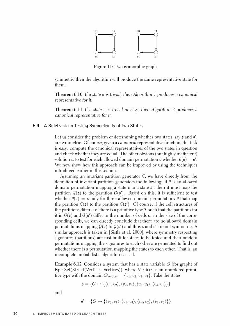
v1 v2

v4 v3

v3 v1

v2 v4

Figure 11: Two isomorphic graphs

symmetric then the algorithm will produce the same representative state forthem.

Theorem 6.10 If a state s is trivial, then Algorithm 1 produces a canonicalrepresentative for it.

Theorem 6.11 If a state s is trivial or easy, then Algorithm 2 produces acanonical representative for it.

6.4 A Sidetrack on Testing Symmetricity of two States

Let us consider the problem of determining whether two states, say s and s′,are symmetric. Of course, given a canonical representative function, this taskis easy: compute the canonical representatives of the two states in questionand check whether they are equal. The other obvious (but highly inefficient)solution is to test for each allowed domain permutation θ whether θ(s) = s′.We now show how this approach can be improved by using the techniquesintroduced earlier in this section.

Assuming an invariant partition generator G, we have directly from thedefinition of invariant partition generators the following: if θ is an alloweddomain permutation mapping a state s to a state s′, then it must map thepartition G(s) to the partition G(s′). Based on this, it is sufficient to testwhether θ(s) = s only for those allowed domain permutations θ that mapthe partition G(s) to the partition G(s′). Of course, if the cell structures ofthe partitions differ, i.e. there is a primitive type T such that the partitions forit in G(s) and G(s′) differ in the number of cells or in the size of the corre-sponding cells, we can directly conclude that there are no allowed domainpermutations mapping G(s) to G(s′) and thus s and s′ are not symmetric. Asimilar approach is taken in [Sistla et al. 2000], where symmetry respectingsignatures (partitions) are first built for states to be tested and then randompermutations mapping the signatures to each other are generated to find outwhether there is a permutation mapping the states to each other. That is, anincomplete probabilistic algorithm is used.

Example 6.12 Consider a system that has a state variable G (for graph) oftype Set(Struct(Vertices,Vertices)), where Vertices is an unordered primi-tive type with the domain DVertices = {v1, v2, v3, v4}. Take the states

s = {G 7→ {〈v1, v2〉, 〈v2, v3〉, 〈v3, v4〉, 〈v4, v1〉}}

and

s′ = {G 7→ {〈v3, v1〉, 〈v1, v4〉, 〈v4, v2〉, 〈v2, v3〉}}


corresponding to the directed graphs shown in Fig. 11. The states are sym-metric since θ =

(θVertices = ( v1 v2 v3 v4

v3 v1 v4 v2 ))

maps s to s′. After applying anyinvariant partition generator G to the states, it must be that the partitionfor Vertices is pVertices = [{v1, v2, v3, v4}] in both partitions G(s) and G(s′).This follows from Fact 5.21 by observing that the stabilizer group Stab(Θ, s)is generated by

(θVertices = ( v1 v2 v3 v4

v2 v3 v4 v1 ))

while Stab(Θ, s′) is generated by(θVertices = ( v1 v2 v3 v4

v4 v3 v1 v2 )).

There are 4! = 24 allowed domain permutations mapping the partitionpVertices in G(s) to the (same) partition pVertices in G(s′). However, by Thm. 3.2there are only |Stab(Θ, s)| = 4 allowed domain permutations mapping s tos′. This example can be extended to graphs with n vertices, where we willhave n! allowed domain permutations mapping the partitions to each otherbut only n of them mapping the states to each other. Thus n! − n of n!,i.e. almost all allowed domain permutations will fail in the symmetry testingapproach described above. ♣

The above symmetricity test can be improved by using search trees. As-

sume that we are given two states, s1 and s2. Take any path G(s1)T1,v1,1−→

p1,1 . . .Tn,v1,n−→ p1,n in the search tree T (s1) ending in a discrete partition p1,n.

Let θ1 be the allowed domain permutation compatible with the leaf partitionp1,n. If s1 and s2 are symmetric, then there is an allowed domain permuta-tion θ mapping s1 to s2 and consequently (by Cor. 6.6) a leaf node θ(p1,n) inthe search tree T (s2,G(s2)). Then by Lemma 5.3, θ1∗θ−1 is compatible withθ(p1,n) and (θ1 ∗ θ−1)(s2) = (θ1 ∗ θ−1)(θ(s1)) = θ1(s1). Furthermore, if θ2

is compatible with a discrete partition p2 in the search tree T (s2,G(s2)) andθ1(s1) = θ2(s2), then (θ−1

2 ∗θ1)(s1) = s2 and the states are symmetric. There-fore, in order to check whether s1 and s2 are symmetric, do a backtrackingsearch in the search tree T (s2) starting from the root node to find whetherthere is a leaf node p2 in it such that the allowed domain permutation θ2 com-patible with p2 maps s2 to θ1(s1). The states s1 and s2 are symmetric iff sucha leaf node can be found. To prune the search tree, note that if θ maps s1 to

s2, then by Cor. 6.4 there is a path θ(G(s1))T1,θT1 (v1,1)−→ θ(p1,1) . . .

T1,θT1 (v1,n)−→θ(p1,n) in the search tree T (s2) and by Lemma 5.3 θ1 ∗ θ−1 is compatiblewith θ(p1,n) and (θ1 ∗ θ−1)(s2) = (θ1 ∗ θ−1)(θ(s1)) = θ1(s1). Therefore, if a

path G(s2)T1,v2,1−→ p2,1 . . .

T1,v2,k−→ p2,k, k < n, is currently being traversed in thesearch tree T (s2), and the cell structures of p1,k and p2,k differ (meaning thatthere cannot be any θ mapping p1,k to p2,k), there is no need to traverse thechildren of the node p2,k. Naturally, this algorithm can be made probabilisticby randomly trying the paths in the search tree T (s2).

Example 6.13 (Ex. 6.12 continued) Applying any reasonably efficient invari-ants, such as those described in Sec. 5.4, in the partition refinerR will makethe search tree for the state s to look something like this:

[{v1}, {v3}, {v4}, {v2}] [{v2}, {v4}, {v1}, {v3}] [{v3}, {v1}, {v2}, {v4}] [{v4}, {v2}, {v3}, {v1}]

[{v1, v2, v3, v4}]


and the search tree for the state s′ is thus:

[{v1, v2, v3, v4}]

[{v1}, {v2}, {v3}, {v4}] [{v2}, {v1}, {v4}, {v3}] [{v4}, {v3}, {v1}, {v2}][{v3}, {v4}, {v2}, {v1}]

Now the domain permutation θ1 =(θVertices

1 = ( v1 v2 v3 v4v1 v4 v2 v3 )

)compatible

with the leftmost leaf node(pVertices = [{v1}, {v3}, {v4}, {v2}]

)of the search

tree for s maps s to θ1(s) = {G 7→ {〈v1, v4〉, 〈v4, v2〉, 〈v2, v3〉, 〈v3, v1〉}}.Now taking any leaf node in the search tree for s′, the allowed domain per-mutation compatible with it maps s′ to θ1(s). For instance, the allowed do-main permutation θ2 =

(θVertices

2 = ( v1 v2 v3 v4v2 v1 v4 v3 )

)compatible with the leaf

node(pVertices = [{v2}, {v1}, {v4}, {v3}]

)of the search tree for s′ maps s′ to

θ2(s′) = {G 7→ {〈v4, v2〉, 〈v2, v3〉, 〈v3, v1〉, 〈v1, v4〉}} = θ1(s). ♣

As the above example shows, using search trees can bring exponential savingsin the symmetricity test approach.

7 HANDLING VERY LARGE AND INFINITE SCALAR SETS

So far we have implicitly assumed that the domains of unordered primitivetypes (scalar sets) are finite. However, it would be convenient to have un-ordered primitive types with infinite domains. For instance, modeling un-bounded resources such as process identifiers would require the domain tobe infinite. Without restrictions, infinite domains cause problems becausepartitions are assumed to be ordered lists of subsets of domains. For instance,if a partition contains two cells that have infinitely many elements and an in-variant would distinguish infinitely many elements in both of these cells, thenthe partition refined according to the invariant would result in an ordered listthat first has infinitely many cells (refined from the first original cell) and af-ter that, yet infinitely many cells (refined from the second original cell). Thisis absurd and would require partitions to be something else than ordered listsor redefining the invariant partitioning process. Likewise, having a cell withinfinitely many elements not as the last cell would invalidate the Def. 5.2 ofcompatible domain permutations.

However, these problem can be circumvented by assuming finite statesin the sense that only finitely many elements in the infinite domain of eachunordered primitive type actually appear in a given state. This is a plausibleassumption since infinitely many elements appearing in a state would alsocause some other problems, starting with the problem of how to representstates. Now consider the allowed domain permutation θ that only swaps twoelements v and v′ of type T not appearing in the state s. Clearly θ(s) = s andG(θ(s)) = θ(G(s)) implies G(s) = θ(G(s)), meaning that the elements v andv′ must belong to the same cell in the partition assigned to s by any invariantpartition generator G. Therefore, invariant partition generators cannot distin-guish between the elements not appearing in a state. Furthermore, if θ′ mapsthe state s to s′, then θ′ ∗ θ also maps s to s′ meaning that it does not matterhow the non-appearing elements are permuted among themselves. Thus we

32 7 HANDLING VERY LARGE AND INFINITE SCALAR SETS

may conclude that we can in effect ignore the elements of unordered primi-tive types that do not appear in the state in question. An algorithmic view ofthis is to first apply the following invariant for each unordered primitive typeT during the computation of the invariant partition generator.

Definition 7.1 The invariant IT,appears(v, s, p) is defined to be 0 if the ele-ment v of a type T appears in the value of any state variable in the state s

(meaning that I]T in x(v, s, p) ≥ 1 for a x ∈ X ), and 1 otherwise.

This splits the elements in the domain of T into two cells: those that appearin the state s (a finite set under the assumption made above) and those thatdo not (an infinite set under the assumption made above). We then ignorethe latter cell. Because we have chosen that the elements appearing in thestate are assigned the value 0 by IT,appears (i.e. have a smaller value than thosenot appearing in the state), the n elements appearing in the state are in thefirst cell and are thus “compressed” into the first n elements in the domainby any allowed domain permutation compatible with the partition producedthis way.

Another view of the same thing is to first apply an allowed domain permu-tation that “compresses” the elements appearing in the domains of infiniteunordered primitive types and then use the algorithms for finite domains de-scribed previously without modification. That is, for a finite state s1, take anyallowed domain permutation θ1 that, for each infinite unordered primitivetype T , maps the n elements in DT appearing in the state s1 to the first nelements in the domain DT . Similarly for another finite state s2. Now thestates s1 and s2 are symmetric iff s′1 = θ1(s1) and s′2 = θ2(s2) are symmetricand if they are, there is an allowed domain permutation that (i) maps θ1(s1)to θ2(s2) and (ii) for each infinite unordered primitive type fixes all the ele-ments not appearing in θ1(s1) or in θ2(s2). We can now reduce the domainsof all infinite unordered primitive types to finite sets consisting only of theelements that appear in the state θ1(s1) or in θ2(s2). Now θ1(s1) and θ2(s2)are symmetric under the allowed domain permutation group for the reduceddomains iff they are under the original allowed domain permutation group.Furthermore, if θ1′(s

′1) = θ2′(s

′2), where θ1′ and θ2′ are allowed domain per-

mutations under the reduced domains, then θ1′(θ1(s1)) = θ2′(θ1(s2)) whenθ1′ and θ2′ are interpreted as if they were allowed domain permutations forthe unreduced domains. Thus the (canonical) representatives computer un-der the reduced domains can be directly used as (canonical) representativesof the original states.

8 ALGORITHMS BASED ON CHARACTERISTIC GRAPHS

Recall Sec. 4 describing characteristic graphs for states. Assuming that wehave an algorithm deciding whether two node labeled, edge weighted di-rected graphs are isomorphic, the obvious algorithm for deciding whethertwo states are symmetric under the group Θ of all allowed domain permuta-tions is to build the characteristic graphs Gs and Gs′ for the two states s and s′

in question and then check whether Gs and Gs′ are isomorphic. (In the caseour graph isomorphism algorithm only supports a weaker form of graphs,

8 ALGORITHMS BASED ON CHARACTERISTIC GRAPHS 33

say node labeled undirected graphs, we have to transform the characteristicgraph into that graph class by replacing edges with additional, appropriatelylabeled vertices.)

We now show how to obtain a canonical representative function for states,provided that we have a canonizer for graphs. Formally, a canonizer forgraphs is a function K from graphs to graphs such that (i) for all graphsG, G and K(G) are isomorphic, and (ii) if two graphs G and G′ are iso-morphic, then K(G) = K(G′). Furthermore, we assume a canonizer thatproduces graphs that have the vertex set drawn from {1, 2, . . . }. That is, ifG has a finite vertex set V , then the canonical form K(G) has the vertex set{1, 2, . . . , |V |}. In addition, it is assumed that an isomorphism κ from Gto K(G) is provided. For instance, the nauty tool [McKay 1990] includes acanonizer that also gives a mapping κ.

A graph canonizer K is extended to KS operating on states as follows.Given a state s, consider its characteristic graph Gs = 〈V, . . .〉. Assume thatκ is a mapping from the vertices of Gs to the vertices of its canonical versionK(Gs). Take the allowed domain permutation θ =

(θT)T∈TP

that is compat-ible with κ, meaning that the following rules are fulfilled.

– For each cyclic primitive type T with DT = {v1, . . . , vn}, consider theset {κ(T ::v) | v ∈ DT} of κ-images of the nodes in the characteristicgraph corresponding to the elements in the domain of T . Now θT is theone that maps the element v ∈ DT having the smallest value κ(T ::v)in the set to v1.

– For each unordered primitive type T with DT = {v1, . . . , vn}, θT isthe one that maps an element v ∈ DT to vi iff v has the ith smallestvalue κ(T ::v).

We denote the state θ(s) by KS(s). The whole algorithm is shown in Alg. 3.The next theorem establishes the correctness of the algorithm.


Output: A canonical representative state for s

Require: A graph canonizer K1: Build the characteristic graph Gs

2: Compute a mapping κ from Gs to its canonical version K(Gs)3: Take the allowed domain permutation θ that is compatible with κ4: Return θ(s) as the canonical representative state

Theorem 8.1 The function KS is a canonical representative function.

Example 8.2 Consider the states s1 = {U 7→ 〈ta, s0〉+〈tb, s3〉, V 7→ s1 + s4}and s2 = {U 7→ 〈ta, s4〉+〈tb, s1〉, V 7→ s2 + s5}. The states are symmetricsince both

θ1 =(θSecs


1 =( ta tb

ta tb

))and

θ2 =(θSecs


2 =( ta tb

tb ta

))34 8 ALGORITHMS BASED ON CHARACTERISTIC GRAPHS

1 1

11

v4v3

v5 v6 v7 v8 v9 v10 v12v11

1 11111

1

v1

var U var V

v2

U V

1 1 2 1 2

11

v4v3

v5 v6 v7 v8 v9 v10 v12v11

1

1 11111

1 1

U Vvar U var V

v1 v2

1 1 2 1 2

(a) Gs1 (b) Gs2

11

2

12 111 11111

1

13 7var U var V

34

1 1

10859614

1 11

1

2 2

(c) K(Gs1) = K(Gs2)

Figure 12: Two characteristic graphs and their common canonical version

map s1 to s2. The characteristic graphs Gs1 and Gs2 of the states are depictedin Figs. 12(a) and 12(b), respectively. In the figures, we use the followingcommon abbreviations for vertex names: v5 = Trains::ta, v6 = Trains::tb,v7 = Secs::s0, v8 = Secs::s1, v9 = Secs::s2, v10 = Secs::s3, v11 = Secs::s4

and v12 = Secs::s5. Assume that a graph canonizer produces the canonicalversion K(Gs1) = K(Gs2) shown in Fig. 12(c) for these characteristic graphs.

There are two isomorphisms from Gs1 to K(Gs1):

κ1,1 =(U V v1 v2 v3 v4 v5 v6 v7 v8 v9 v10 v11 v1213 7 4 3 1 2 11 12 6 9 5 8 10 14

)and


).

The two allowed domain permutations compatible with these isomorphismsare

θs1,1 =(θSecs

s1,1= ( s0 s1 s2 s3 s4 s5

s4 s5 s0 s1 s2 s3 ) , θTrainss1,1

=( ta tb

ta tb

))and

θs1,2 =(θSecs

s1,2= ( s0 s1 s2 s3 s4 s5


=( ta tb

tb ta

)),

respectively. The canonical representative state for s1 is thus

KS(s1) = θs1,1(s1) = θs1,2(s1) = {U 7→ 〈ta, s4〉+〈tb, s1〉, V 7→ s2 + s5}.

Similarly, there are two isomorphisms from Gs2 to K(Gs2):


)and


).

The two allowed domain permutations compatible with these isomorphismsare

θs2,1 =(θSecs

s2,1= ( s0 s1 s2 s3 s4 s5


=( ta tb

ta tb

))and

θs2,2 =(θSecs

s2,2= ( s0 s1 s2 s3 s4 s5


=( ta tb

tb ta

)),

8 ALGORITHMS BASED ON CHARACTERISTIC GRAPHS 35

respectively. The canonical representative state for s2 is thus

KS(s2) = θs2,1(s2) = θs2,2(s2) = {U 7→ 〈ta, s4〉+〈tb, s1〉, V 7→ s2 + s5}

which equals to KS(s1). ♣

Note that the algorithms Alg. 1 and Alg. 3 could be combined as follows.Given a state, first compute the partition G(s) for it by using a fixed invariantpartition generator G. If G(s) is discrete, then return the state θ(s) as thecanonical representative state, where θ is the allowed domain permutationcompatible with G(s). If

(pT)T∈TP

= G(s) is not discrete, build the char-acteristic graph Gs. Then change the label of each vertex of form T ::v for apermutable primitive type T from T to T.incell(pT , v), and proceed to line2 of algorithm Alg. 3.

9 SOME EXPERIMENTAL RESULTS

We have implemented the algorithms proposed in this report in the version3.1 of the Murϕ tool. In this section we present some experimental results onthe example systems in the Murϕ distribution as well as on some others. Theoriginal Murϕ tool has four representative algorithms, described by the helppage of the tool and in [Ip 1996]. The first one simply applies all the alloweddomain permutations to the state in question and returns the smallest stateobtained as the canonical representative state. The other three algorithmsfirst build an ordered partition as in this text by using some invariants andthen apply all, 10, or 1, respectively, domain permutations compatible withthe partition to the state and return the smallest state found this way as therepresentative state. The algorithm Alg. 1 in this work is basically the lastMurϕ algorithm except that we use more powerful invariants for buildingthe partition. In more detail, the invariant partition generator in algorithmsAlg. 1 and Alg. 2 is obtained as follows. First, we apply the invariants forordered structured types described in Sec. 5.4 on state variables if possible.Then, for the other state variables, we apply the hash-like invariants describedin Sec. 5.4 until no refinement occurs. In algorithm Alg. 2, the appliedpartition refiner is produced by refining with the hash-like invariants.

In addition to the example systems in the Murϕ distribution, we use thefollowing graph enumeration systems inspired by the proof of Thm. 3.4 in[Ip 1996]. Figure 13 shows a Murϕ program called graphs5.m. It has theunordered primitive type (scalar set) called Vertex with the domain of size5 for the vertices of a graph, and one state variable called edges of typeAssocArray(Vertex,AssocArray(Vertex,Bool)) with the intuition that eachvertex is associated with each vertex and a Boolean value describing whetherthere is an edge from the first vertex to the second one. The initial stateis such that all the edges except self-loops are in it. The transition (rule)“Delete Edge” then removes one (undirected) edge, meaning that the reach-ability graph of the system consists of all the self-loopless (undirected) graphswith 5 vertices. Consequently, the (optimal) symmetry reduced reachabil-ity graph consists of all such graphs up to isomorphism. Changing the rule“Delete Edge” into

36 9 SOME EXPERIMENTAL RESULTS

Ruleset i:Vertex doRuleset j:Vertex doRule "Delete edge"edges[i][j]=TRUE ==> edges[i][j] := FALSE;

EndRule;EndRuleset;EndRuleset;

results in system called digraphs5.m, enumerating all the directed graphs of5 vertices.constnof_vertices: 5;typeVertex: scalarset(nof_vertices);varedges: Array[Vertex] of Array[Vertex] of boolean;StartstateBeginfor i:Vertex do for j:Vertex doif(i!=j) then edges[i][j] := true; else edge s[i][j]:=false; end;

end; end;End;

Ruleset i:Vertex doRuleset j:Vertex doRule "Delete edge"edges[i][j]=TRUE ==> edges[i][j] := FALSE; edges[j][i] := FALSE;EndRule;EndRuleset;EndRuleset;

Invariant "dummy"TRUE

Figure 13: A graph enumeration system

Table 1 shows the data of the experiments, run in an AMD Athlon 1GHzprocessor powered PC machine under the Linux operating system. The run-ning times reported are in seconds. Note that the Murϕ algorithms 1 and 2as well as algorithm Alg. 3 are canonical representative functions and thusthe state columns for these algorithms give the size of the optimally reducedreachability graph.

As the Murϕ examples (from adash to n_peterson) show, algorithm Alg. 1is quite fast and produces almost optimally reduced reachability graphs inthese examples. In some cases it produces considerably smaller number ofstates than the original Murϕ algorithm 4, which is due to the use of morepowerful invariants, especially the hash-like invariants described in Sec. 5.4.Usually it slightly outperforms (in terms of generated states) even the Murϕalgorithm 3 which has an advantage of trying 10 permutations instead ofjust selecting an arbitrary one. Interestingly, the algorithm Alg. 2 producesoptimally reduced reachability graphs for these instances although it is nota canonical representative algorithm. Furthermore, it is not significantlyslower than algorithm Alg. 1.

In the graph enumeration problems (graphn and digraphn), the algo-rithms Alg. 1 and 2 perform very well, producing reachability graphs that

9 SOME EXPERIMENTAL RESULTS 37

are reasonably close to the optimal ones. Again, especially the algorithmAlg. 2 produces nearly optimal results in reasonably short time. The Murϕalgorithms 2–4 do not perform very well because the invariants implementedin the standard Murϕ tool cannot do anything in these systems. Note thatalthough the number of states in the reduced reachability graphs can be verysmall, the number of times the representative function is called can be muchbigger. For instance, on the problem instance graph8 the algorithm Alg. 2produces a reachability graph with 12376 states but with 346528 edges (exe-cuted transitions), meaning that the representative function is actually called346528 times during the reachability graph generation.

We have also implemented the algorithm Alg. 3 by using the nauty tool[McKay 1990] as the graph canonizer. The bad experimental results shownin Table 1 are probably due to the fact that the characteristics graphs of statesare quite large. The graphs can be large to begin with, and in addition, asnauty is specially optimized for undirected graphs having no edge weights,we had to add some nodes into the graphs in order to use nauty. As an ex-ample, the nauty version of the characteristic graph of a state in the eadashinstance has 2768 vertices. Furthermore, the nauty tool is designed for densegraphs — the graphs are represented as adjacency matrixes. Thus a charac-teristic graph of a state in the eadash instance takes almost one megabyte ofmemory to represent. This considerably slows down the partition refinementalgorithms in nauty. Therefore, even though the search tree for the charac-teristic graph of a state in nauty is usually very small, it may take a lot of timeto compute it. The results for algorithm Alg. 3 might look different if we hada graph canonizer designed for directed, edge weighted, and sparse graphs.

10 SOME RELATED WORK

The algorithms in the Murϕ tool were already discussed in the previous sec-tion. The main difference between Alg. 1 and the Murϕ algorithms is that weuse more powerful invariants, especially the hash-like invariants in Sec. 5.4are novel. Furthermore, we also handle cyclic primitive types (non-reflexivering symmetries in the Murϕ terminology) in a unified way. The two otheralgorithm presented in this report are new.

The approach taken in [Sistla et al. 2000] is discussed in Sec. 6.4.In [Huber et al. 1985; Jensen 1995] a very elementary version of the parti-

tion refinement process is given and applied to checking whether two mark-ings of a colored Petri net are symmetric. Especially, no other structuredtypes than of form Multi-Set(T ), where T is an unordered primitive type, arehandled.

Recently, an approach based on computational group theory was pre-sented in [Lorentsen and Kristensen 2001]. The idea there is that, givena state s, first compute the stabilizer group Stab(Θ, s) and then check all the|Θ| / |Stab(Θ, s)| left coset representative permutations of Stab(Θ, s) in Θand select the smallest state obtained as the canonical representative state.When |Stab(Θ, s)| is large, substantial savings can be obtained comparedto the approach in which all permutations in Θ are tested. However, when-ever |Stab(Θ, s)| is very small, no such large savings are obtained; especially

38 10 SOME RELATED WORK

system Murϕ Murϕ Murϕ Murϕname alg. 1 alg. 2 alg. 3 alg. 4

states time states time states time states timeadash 10466 7 10466 7 10466 7 10471 7

cache3 31433 88 31433 8 31433 5 31433 5eadash 133426 524 133426 374 133480 423 191088 378ldash 254743 542 254743 403 254974 423 314194 447

mcslock1 23636 3 23636 3 23645 3 24668 3mcslock2 540219 57 540219 63 540219 64 542071 61

list6 23410 7 23410 2 23410 2 23446 2n_peterson 163298 5341 163298 42 163298 42 163298 42digraphs3 16 1 16 1 16 1 64 1digraphs4 218 1 218 1 554 1 4096 1digraphs5 9608 111 9608 116 142113 392 >381000 >1hgraphs5 34 1 34 1 183 1 1024 1graphs6 156 34 156 23 5408 12 32768 14graphs7 1044 1963 1044 2008 >105000 >1h >141000 >1hgraphs8 >210 >1h >210 >1h >257000 >1h >335000 >1h

system algorithm algorithm algorithmname Alg. 1 Alg. 2 Alg. 3

states time states time states timeadash 10466 7 10466 7 10466 9766

cache3 31433 5 31433 5 31433 556eadash 133439 312 133426 311 >200 >1hldash 254755 356 254743 354 >1030 >1h

mcslock1 23644 2 23636 2 23636 33mcslock2 540220 47 540219 47 540219 735

list6 23410 2 23410 2 23410 62n_peterson 163298 32 163298 35 163298 420digraphs3 16 1 16 1 16 1digraphs4 228 1 218 1 218 1digraphs5 9832 5 9616 5 9608 54graphs5 40 1 34 1 34 1graphs6 243 1 156 1 156 5graphs7 1683 5 1046 4 1044 63graphs8 19601 99 12376 67 12346 1556

Table 1: Some experimental results

in systems in which most of the reachable states have no self-symmetriesi.e. |Stab(Θ, s)| = 1, all the permutations are tested in most of the cases.Note that the states for which |Stab(Θ, s)| is very small are also the statesfor which the symmetry reduction method has the largest reduction pos-sibility: the number |Θ| / |Stab(Θ, s)| of symmetric states that can be ig-nored is large. An advantage of this algorithm is that, as it gives the sta-bilizer group Stab(Θ, s), some transitions starting from s can be prunedaway (never executed) because they will lead to symmetric successor states.However, note that computing the group Stab(Θ, s) is in general as hardas finding the automorphism group of a graph (a task for which we do notknow any polynomial time algorithm). In [Lorentsen and Kristensen 2001],the stabilizer group Stab(Θ, s) is basically found iteratively by letting Θ1 =Stab(Θ, s(x1)), Θ2 = Stab(Θ1, s(x2)), . . . , and Θn = Stab(Θn−1, s(xn)),where x1, . . . , xn are the state variables. Now Θn = Stab(Θ, s). The back-tracking algorithm presented in [Butler 1991] is used to compute each of the

10 SOME RELATED WORK 39

groups Stab(Θi, s(xi+1)). However, we could probably compute the stabi-lizer group Stab(Θ, s) and the lexicographically smallest state symmetric tos (i.e. a canonical representative state for s) at the same time by the followingprocedure. Assuming the state variables x1, . . . , xn, initialize the left cosetθ0 ∗ Θ0 to be I ∗ Θ, where I is the identity domain permutation. Let θi bea domain permutation in the coset θi−1 ∗ Θi−1 that has minimal θi(s(xi))(the domains of types are assumed to be totally ordered). The coset after theith round is then θi ∗ Θi, where Θi = Stab(Θi−1, s(xi)). Now θn ∗ Θn is acanonical labeling coset, where θn(s) is the lexicographically smallest statesymmetric to s and Θn = Stab(Θ, s). Now a variant of the backtracking al-gorithm presented in [Butler 1991] is not only used to compute each of thegroups Θi = Stab(Θi−1, s(xi)) but also the domain permutation θi in thecoset θi−1 ∗Θi−1 that has minimal θi(s(xi)).

In [Chiola et al. 1991] an algorithm is presented for computing a symbolicrepresentative marking for each encountered marking in the context of Well-Formed Nets (WFNs).

11 CONCLUSIONS

In this report we have presented symmetry reduction algorithms under datatype symmetries. The first two algorithms resemble the preprocessing andsearch phases, respectively, of common graph isomorphism checking algo-rithms. The first algorithm, given a state, produces an ordered partition of theelements of the permutable primitive types, selects one permutation based onthe partition and returns the permuted state as the representative state. Thedifference between the existing algorithms in the Murϕ tool [Ip 1996] andthe first algorithm is that more powerful invariants are used to obtain theordered partition. The second algorithm improves the first one by selectingan arbitrary path in the search tree whose root is the partition produced inthe first algorithm and then returns the state permuted with the permutationassociated with the leaf partition as the representative state. The third al-gorithm presented exploits the characteristic graphs of states, i.e. graphs thatare isomorphic iff the corresponding states are symmetric. The existing graphisomorphism/canonicalization algorithms are then used to canonicalize thecharacteristic graph of a state, resulting in the canonical representative statefor the state. Some experimental results were also presented, showing thatthe algorithms are competitive against the previous ones implemented in theMurϕ tool.

Acknowledgements

The author wishes to thank the Helsinki Graduate School in ComputerScience and Engineering (HeCSE) and the Academy of Finland (projectsno. 47754 and no. 43963) for their financial support and Petteri Kaski for hiscomments on this work.

40 11 CONCLUSIONS

References

BUTLER, G. 1991. Fundamental Algorithms for Permutation Groups. Lecture Notes inComputer Science, vol. 559. Springer-Verlag, Berlin, Germany.

CHIOLA, G., DUTHEILLET, C., FRANCESCHINIS, G., AND HADDAD, S. 1991. Onwell-formed coloured nets and their symbolic reachability graph. See Jensen andRozenberg [1991], 373–396.

CLARKE, E. M., GRUMBERG, O., AND PELED, D. A. 1999. Model Checking. TheMIT Press, Cambridge, Massachusetts.

GENRICH, H. J. 1991. Predicate/transition nets. See Jensen and Rozenberg [1991], 3–43.

HUBER, P., JENSEN, A. M., JEPSEN, L. O., AND JENSEN, K. 1985. Towards reacha-bility trees for high-level Petri nets. Tech. Rep. DAIMI PB 174, Datalogisk Afdeling,Matematisk Institut, Aarhus Universitet. May.

IP, C. N. 1996. State reduction methods for automatic formal verification. Ph.D. thesis,Department of Computer Science, Stanford University.

IP, C. N. AND DILL, D. L. 1996. Better verification through symmetry. Formal Methodsin System Design 9, 1/2 (Aug.), 41–76.

JENSEN, K. 1995. Coloured Petri Nets: Basic Concepts, Analysis Methods and PracticalUse: Volume 2, Analysis Methods. Monographs in Theoretical Computer Science.Springer.

JENSEN, K. AND ROZENBERG, G., Eds. 1991. High-level Petri Nets; Theory and Appli-cation. Springer.

JUNTTILA, T. 1999. Detecting and exploiting data type symmetries of algebraic systemnets during reachability analysis. Research Report A57, Helsinki University of Tech-nology, Laboratory for Theoretical Computer Science, Espoo, Finland. Dec.

KREHER, D. L. AND STINSON, D. R. 1999. Combinatorial Algorithms: Generation,Enumeration and Search. CRC Press, Boca Raton, Florida, USA.

LORENTSEN, L. AND KRISTENSEN, L. M. 2001. Exploiting stabilizers and parallelismin state space generation with the symmetry method. In Proceedings of the SecondInternational Conference on Application of Concurrency to System Design (ACSD2001). IEEE Computer Society, 211–220.

MCKAY, B. D. 1981. Practical graph isomorphism. Congressus Numerantium 30, 45–87.

MCKAY, B. D. 1990. Nauty user’s guide (version 1.5). Tech. Rep. TR-CS-90-02, Com-puter Science Department, Australian National University.

SISTLA, A. P., GYURIS, V., AND EMERSON, E. A. 2000. SMC: A symmetry-basedmodel checker for verification of safety and liveness properties. ACM Transactionson Software Engineering and Methodology 9, 2 (Apr.), 133–166.

VALMARI, A. 1998. The state explosion problem. In Lectures on Petri Nets I: Basic Mod-els, W. Reisig and G. Rozenberg, Eds. Lecture Notes in Computer Science, vol.1491. Springer, 429–528.

A PROOFS

Proof of Theorem 3.2

Theorem 3.2 Assume a domain permutation ψ ∈ Ψ that maps a state s1 tos2 i.e. ψ(s1) = s2. Then

1. Stab(Ψ, s2) = ψ ∗ Stab(Ψ, s1) ∗ ψ−1, where ψ ∗ Stab(Ψ, s1) ∗ ψ−1 ={ψ ∗ ψ′ ∗ ψ−1 | ψ′ ∈ Stab(Ψ, s1)}, and

A PROOFS 41

2. the left coset ψ ∗ Stab(Ψ, s1) = {ψ ∗ ψ′ | ψ′ ∈ Stab(Ψ, s1)} is exactlythe set of all domain permutations in Ψ mapping s1 to s2.

Consequently, (i) |Stab(Ψ, s1)| = |Stab(Ψ, s2)|, (ii) there are |Stab(Ψ, s1)|domain permutations mapping s1 to s2, and (iii) there are |Ψ| / |Stab(Ψ, s1)|states that are Ψ-symmetric to s1.

Proof. Part 1. If ψ′ ∈ Stab(Ψ, s1), then (ψ ∗ ψ′ ∗ ψ−1)(s2) = (ψ ∗ ψ′)(s1) =ψ(s1) = s2 implying that ψ ∗ ψ′ ∗ ψ−1 ∈ Stab(Ψ, s2) and Stab(Ψ, s2) ⊇ψ ∗ Stab(Ψ, s1) ∗ ψ−1. On the other hand, if ψ′′ ∈ Stab(Ψ, s2), thenψ−1 ∗ ψ′′ ∗ ψ ∈ Stab(Ψ, s1) and ψ′′ ∈ ψ ∗ Stab(Ψ, s1) ∗ ψ−1 implying thatStab(Ψ, s2) ⊆ ψ ∗ Stab(Ψ, s1) ∗ ψ−1.

Part 2. Each domain permutation in the left coset ψ ∗ Stab(Ψ, s1) mapss1 to s2 since (ψ ∗ ψ′)(s1) = ψ(s1) = s2 whenever ψ′ ∈ Stab(Ψ, s1). Onthe other hand, assume that ψ′′(s1) = s2 for a domain permutation ψ′′ ∈ Ψ.Thus (ψ−1 ∗ ψ′′)(s1) = ψ−1(s2) = s1 implying that ψ−1 ∗ ψ′′ ∈ Stab(Ψ, s1).But now ψ ∗ (ψ−1 ∗ ψ′′) = ψ′′ belongs to the left coset ψ ∗ Stab(Ψ, s1). �

Proof of Lemma 5.3

Lemma 5.3 Let θ be an allowed domain permutation compatible with apartition p. Then for each allowed domain permutation θ it holds that theallowed domain permutation θ ∗ θ−1 is compatible with the partition θ(p).

Proof. Let θ =(θT)T∈TP

, p =(pT)T∈TP

, and pT = [CT1 , . . . , C

TcT

].

For a cyclic primitive type T , assume that θT maps a vi ∈ CT1 to v1,

i.e. θT (vi) = v1. Observe that θT = θT ◦ θT−1 ◦ θT and therefore (θT ◦θT−1

)(θT (vi)) = v1. But now θT (vi) is in the first cell for the type T in thepartition θ(p) and thus θ∗θ−1 fulfills the compatibility requirement w.r.t. θ(p)for the type T .

For an unordered primitive type T , assume that for vi, vj ∈ DT it holdsthat incell(θT (pT ), vi) < incell(θT (pT ), vj). Thus incell(pT , θT

−1(vi)) <

incell(pT , θT−1

(vj)) holds, too. As θ is compatible with p, θT (θT−1

(vi)) =

vi′ = (θT ◦ θT−1)(vi) and θT (θT

−1(vj)) = vj′ = (θT ◦ θT−1

)(vj) such thati′ < j′, and thus θ ∗ θ−1 fulfills the compatibility requirement w.r.t. θ(p) forthe type T . �

Proof of Corollary 5.4

Corollary 5.4 Assume an invariant partition generator G, and take two sym-metric states, s1 and s2. Let θ1 be an allowed domain permutation compat-ible with the partition G(s1). Then there is an allowed domain permutationθ2 compatible with the partition G(s2) such that θ1(s1) = θ2(s2).

Proof. First, there is an allowed domain permutation θ2 such that θ1(s1) =

θ2(s2). This is because s1 and s2 are symmetric and therefore there is anallowed domain permutation θ such that θ(s1) = s2. Thus the requirementθ1(s1) = θ2(s2) is equivalent to θ1(s1) = θ2(θ(s1)) = (θ2 ∗θ)(s1). Obviously,θ2 = θ1 ∗ θ−1 is a solution to this. Second, since G is an invariant partition

42 A PROOFS

generator, G(s2) = G(θ(s1)) = θ(G(s1)). By Lemma 5.3, θ2 = θ1 ∗ θ−1 iscompatible with G(s2) = θ(G(s1)) because θ1 is compatible with G(s1). �

Proof of Lemma 5.7

Lemma 5.7 The composition R1 ?R2 of two partition refiners R1 and R2,defined by (R1 ?R2)(s, p) = R2(s,R1(s, p)), is a partition refiner.

Proof. Clearly pref = (R1 ?R2)(s, p) = R2(s,R1(s, p)) is a cell order pre-serving refinement of p since R2(s,R1(s, p)) � R1(s, p) � p. On the otherhand, θ((R1 ? R2)(s, p)) = θ(R2(s,R1(s, p))) = R2(θ(s), θ(R1(s, p))) =R2(θ(s),R1(θ(s), θ(p))) = (R1 ?R2)(θ(s), θ(p)). �


Theorem 5.8 For a partition refiner R, the function GR(s) = R(s, p0),where p0 =

(pT0 = [DT ]

)T∈TP

, is an invariant partition generator.

Proof. Observe that θ(p0) = p0 for any allowed domain permutation θ. ThusGR(θ(s)) = R(θ(s), p0) = R(θ(s), θ(p0)) = θ(R(s, p0)) = θ(GR(s)). �

Proof of Lemma 5.11

Lemma 5.11 If I is a type invariant for a primitive type T in a type T ′ and xis a state variable of type T ′, then Ix(v, s, p) = I(v, s(x), p) is an invariant forT .

Proof. For all θ ∈ Θ, Ix(θT (v), θ(s), θ(p)) = I(θT (v), (θ(s))(x), θ(p)) =I(θT (v), θT

′(s(x)), θ(p)) = I(v, s(x), p) = Ix(v, s(x), p). �

Proof of Lemma 5.14

Lemma 5.14 The functionRI is a partition refiner.

Proof. The fact that RI(s, p) � p follows directly from the items 2(a) and2(b) of the definition.

Take any state s, any partition p =(pT)T∈TP

, and any allowed domainpermutation θ =

(θT)T∈TP

. We must show that θ(R(s, p)) = R(θ(s), θ(p)).First, consider any primitive type T ′ 6= T . Since the invariant I is for the

type T , (i) the partition for a T ′ in the partition R(s, p) is pT , and (ii) thepartition for a T ′ in the partitionR(θ(s), θ(p)) is θ(pT ).

Now consider the partitions for the type T inR(s, p) and inR(θ(s), θ(p)).Take any two elements v, v′ ∈ DT . Now it suffices to notice the following:

1. v and v′ belong to the same cell in the partition pT iff θT (v) and θT (v′)belong to the same cell in the partition θ(pT ),

2. v belongs to an earlier cell than v′ in pT iff θT (v) belongs to an earliercell than θT (v′) in θ(pT ),

3. I(v, s, p) = I(v′, s, p) iff I(θT (v), θ(s), θ(p)) = I(θT (v′), θ(s), θ(p)),and

4. I(v, s, p) < I(v′, s, p) iff I(θT (v), θ(s), θ(p)) < I(θT (v′), θ(s), θ(p)).

A PROOFS 43

Thus CTi is the ith cell in the partition for the type T inR(s, p) iff θT (CT

i ) isthe ith cell in the partition for the type T inR(θ(s), θ(p)). �

Proof of Lemma 5.16

Lemma 5.16 The function IT,succ is an invariant.

Proof. Assume that succT (v) belongs to the ith cell in the partition pT . Thenfor an allowed domain permutation θ =

(θT)T∈TP

in which θT = succkT fora 1 ≤ k ≤ |DT |, succkT (succT (v)) = succT (succkT (v)) = succT (θT (v))belongs to the ith cell in the partition θ(pT ). �

Proof of Lemma 5.18

Lemma 5.18 If θ =(θT)T∈T is an allowed domain permutation, then

gT (v, T ′, v′, p) = gT (θT (v), T ′, θT′(v′), θ(p)).

Proof. By induction on the structure of T ′.Induction base. Assume an allowed domain permutation θ =

(θT)T∈T .

1. For an ordered primitive type T ′,

gT (θT (v), T ′, θT′(v′), θ(p)) = hT ′(θ

T ′(v′))

= hT ′(v′)

= gT (v, T ′, v′, p)

since θT ′(v′) = v′ for an ordered primitive type T ′.2. Let T ′ be a cyclic primitive type with DT ′ = {v1, . . . , vn}.

(a) If T 6= T ′, then

gT (θT (v), T ′, θT′(v′), θ(p)) = hT ′(incell(θ(pT

′), θT

′(v′)))

= hT ′(incell(pT′, v′))

= gT (v, T ′, v′, p).

(b) If T = T ′, then

gT (θT (v), T ′, θT′(v′), θ(p)) = hT ′,2(k, incell(θ(pT

′), θT

′(v′)))

= hT ′,2(k, incell(pT′, v′))

= gT (v, T ′, v′, p)

because v′ is the k-successor of v iff θT (v′) is the k-successor ofθT (v).

3. Let T ′ be an unordered primitive type.(a) If T 6= T ′ or T = T ′ ∧ v 6= v′, then

gT (θT (v), T ′, θT′(v′), θ(p)) = hT ′,2(incell(θ(pT

′), θT

′(v′)), 0)

= hT ′,2(incell(pT′, v′), 0)

= gT (v, T ′, v′, p).

Note that in the case T = T ′, v 6= v′ iff θT (v) 6= θT (v′).

44 A PROOFS

(b) If T = T ′ and v = v′, then

gT (θT (v), T ′, θT′(v′), θ(p)) = hT ′,2(incell(θ(pT

′), θT

′(v′)), 1)

= hT ′,2(incell(pT′, v′), 1)

= gT (v, T ′, v′, p).

Again, if T = T ′, then v = v′ iff θT (v) = θT (v′).

Induction hypothesis. Assume that the lemma holds for types T1, . . . ,Tn.Induction step.

– For a list type T ′ = List(T1),

gT (θT (v), T ′, θT′(〈v1, . . . , vn〉), θ(p)) =

gT (θT (v), T ′, 〈θT1(v1), . . . , θT1(vn)〉, θ(p)) =hT ′,n(gT (θT (v), T1, θ

T1(v1), θ(p)), . . . , gT (θT (v), T1, θT1(vn), θ(p))) =

hT ′,n(gT (v, T1, v1, p), . . . , gT (v, T1, vn, p)) =gT (v, T ′, 〈v1, . . . , vn〉, p).

– For a structure type T ′ = Struct(T1, . . . , Tn),

gT (θT (v), T ′, θT′(〈v1, . . . , vn〉), θ(p)) =

gT (θT (v), T ′, 〈θT1(v1), . . . , θTn(vn)〉, θ(p)) =hT ′,n(gT (θT (v), T1, θ

T1(v1), θ(p)), ..., gT (θT (v), Tn, θTn(vn), θ(p))) =hT ′,n(gT (v, T1, v1, p), . . . , gT (v, Tn, vn, p)) =

gT (v, T ′, 〈v1, . . . , vn〉, p).

– For a set type T ′ = Set(T1),

gT (θT (v), T ′, θT′(v′), θ(p)) =

hT ′

⊕v′′∈θT ′ (v′)

gT (θT (v), T1, v′′, θ(p))

=

hT ′

⊕θT1 (v′′)∈θT ′ (v′)

gT (θT (v), T1, θT1(v′′), θ(p))

=

hT ′

⊕θT1 (v′′)∈θT ′ (v′)

gT (v, T1, v′′, p)

=

hT ′

(⊕v′′∈v′

gT (v, T1, v′′, p)

)=

gT (v, T ′, v′, p)

by using the commutativity and associativity of ⊕, and by noticing thatfor all v′ ∈ DSet(T1) and all v′′ ∈ DT1 , v′′ ∈ v′ iff θT1(v′′) ∈ θSet(T1)(v′).

– Assume that T ′ = Multi-Set(T1). Now an element v′′ ∈ DT1 has mul-tiplicity n in a multi-set v′ ∈ DMulti-Set(T1) iff the element θT1(v′′) hasmultiplicity n in the multi-set θT ′(v′). The rest of the proof is similar tothe previous case.

A PROOFS 45

– Let T ′ = AssocArray(T1, T2). Now for each v′ ∈ DAssocArray(T1,T2), apair 〈v1, v2〉 ∈ v′ iff 〈θT1(v1), θT2(v2)〉 ∈ θT ′(v′). The rest of the proofis similar to the case T ′ = Set(T1).

– For an union type T ′ = Union(T1, . . . , Tn),

gT (θT (v), T ′, θT′(〈Ti, v′〉), θ(p)) = gT (θT (v), T ′, 〈Ti, θTi(v′)〉, θ(p))

= hT ′(gT (θT (v), Ti, θTi(v′), θ(p)))

= hT ′(gT (v, Ti, v′, p))

= gT (v, T ′, 〈Ti, v′〉, p).

�


Theorem 6.3 For each allowed domain permutation θ, a partition pchild is av-child of the root node of the search tree T (s, p) iff the partition θ(pchild) isa θT (v)-child of the root node of the search tree T (θ(s), θ(p)).

Proof. If p is discrete, then T (s, p) has no children. But now θ(p) is alsodiscrete and T (θ(s), θ(p)) has no children.

Clearly, pT = [CT1 , C

T2 , . . . ] is the first non-discrete partition in p iff

θ(pT ) = [θT (CT1 ), θT (CT

2 ), . . . ] is the first non-discrete partition in θ(p).Furthermore, CT

i = {vi,1, vi,2, . . . } is the first non-singleton cell in pT iffθT (CT

i ) = {θT (vi,1), θT (vi,2), . . . } is the first non-singleton cell in θ(pT ).Now the root node p of the tree T (s, p) has as its children the nodesR(s, pj),where for each 1 ≤ j ≤

∣∣CTi

∣∣ the partition pj is the same as p except that thepartition for T is

pTj = [CT1 , . . . , C

Ti−1, {vi,j}, CT

i \ {vi,j}, CTi+1, . . . ].

But the root node θ(p) of the tree T (θ(s), θ(p)) has as its children the nodesR(θ(s), pj′), where for each 1 ≤ j ≤

∣∣θT (CTi )∣∣ =

∣∣CTi

∣∣ the partition pj′ isthe same as θ(p) except that the partition for T is

pTj′ = [θT (CT1 ), . . . , θT (CTi−1), {θT (vi,j)}, θT (CTi ) \ {θT (vi,j)}, θT (CTi+1), . . . ]

which equals to θ(pTj ). Thus the root node θ(p) of the tree T (θ(s), θ(p)) hasas its children the nodes R(θ(s), θ(pj)) = θ(R(s, pj)), meaning that pchild isa vi,j -child of T (s, p) iff θ(pchild) is a θT (vi,j)-child of T (θ(s), θ(p)). �

Proof of Lemma 6.8

Lemma 6.8 For any allowed domain permutation θ, ST (s,p) = ST (θ(s),θ(p))

and consequently ST (s) = ST (θ(s))

Proof. For all allowed domain permutations θ, (i) by Cor. 6.5 a partitionpleaf is a leaf node in T (s, p) iff θ(pleaf) is a leaf node in T (θ(s), θ(p)), (ii) θis compatible with pleaf iff θ ∗ θ−1 is compatible with the partition θ(pleaf) (byLemma 5.3 and the fact that pleaf is discrete), and (iii) thus (θ ∗ θ−1)(θ(s)) =θ(s) ∈ ST (θ(s),θ(p)) iff θ(s) ∈ ST (s,p). �

46 A PROOFS

Proof of Lemma 6.9

Lemma 6.9 If a state s is trivial/easy/hard, then θ(s) is also trivial/easy/hardfor any allowed domain permutation θ.

Proof. If a state s is trivial, then the search tree T (s,G(s)) contains only onenode, i.e. G(s) is a discrete partition. But now for any allowed domain per-mutation θ, it must be that G(θ(s)) = θ(G(s)), which is a discrete partition,and thus the search tree T (θ(s),G(θ(s))) contains only one node and θ(s) isalso trivial.

Now assume that a state s is easy and take any allowed domain permu-tation θ. Now the search tree T (θ(s),G(θ(s))) must contain more than onenode: if it contained only one node, θ(s) would be trivial and by the previouscase θ−1(θ(s)) = s would also be trivial, which contradicts the assumptionthat s is easy. Take any two leaf nodes, say p1′ and p2′ , in the search treeT (θ(s),G(θ(s))). By Corollary 6.6, θ−1(p1′) and θ−1(p2′) are leaf nodes inthe search tree T (s,G(s)). Since s is easy, there is a self-symmetry θself-symm

of s such that θself-symm(θ−1(p1′)) = θ−1(p2′). Now θ ∗ θself-symm ∗ θ−1 is aself-symmetry of θ(s) and (θ ∗ θself-symm ∗ θ−1)(p1′) = θ(θself-symm(θ−1(p1′))) =θ(θ−1(p2′)) = p2′ . Thus θ(s) is also easy.

If a state s is hard, then the state θ(s) must also be hard for any allowed do-main permutation θ. For if θ(s) were trivial (easy), then by the previous casesθ−1(θ(s)) = s would also be trivial (easy), which contradicts the assumptionthat s is hard. �


Theorem 6.10 If a state s is trivial, then Algorithm 1 produces a canonicalrepresentative for it.

Proof. Since s is trivial, the partition G(s) is a discrete partition, there is aunique allowed domain permutation θ compatible with G(s), and the rep-resentative state is θ(s). For any allowed domain permutation θ, θ(s) isalso trivial, the partition G(θ(s)) = θ(G(s)) is discrete, θ ∗ θ−1 is com-patible with θ(G(s)) by Lemma 5.3 and the representative state for θ(s) is(θ ∗ θ−1)(θ(s)) = θ(s). �


Theorem 6.11 If a state s is trivial or easy, then Algorithm 2 produces acanonical representative for it.

Proof. The case in which s is trivial follows directly from Thm. 6.10. Nowassume that s is easy.

We first have to show that choosing any path in the search tree T (s,G(s))leads to the same representative state for s. Take any two leaf nodes, sayp1 and p2, in the search tree T (s,G(s)). Since s is easy, there is a self-symmetry θ mapping p1 to p2, i.e. θ(p1) = p2. If θ is the unique alloweddomain permutation compatible with p1, then θ ∗ θ−1 is the unique alloweddomain permutation compatible with θ(p1) = p2 by Lemma 5.3. But now

A PROOFS 47

(θ ∗ θ−1)(s) = θ(θ−1(s)) = θ(s) since θ−1 is a self-symmetry of s because θis.

Finally, we have to show that for any allowed domain permutation θ, therepresentative state for the easy state θ(s) is the same as the representativestate for s. Take any leaf node p1′ in the search tree T (θ(s),G(θ(s))) andthe unique allowed domain permutation θ1′ compatible with p1′ . By Corol-lary 6.6, θ−1(p′1) is a leaf node in the search tree T (s,G(s)). By Lemma 5.3,θ1′ ∗ (θ−1)−1 = θ1′ ∗θ is the unique allowed domain permutation compatiblewith θ−1(p′1). But now (θ1′ ∗ θ)(s) = θ1′(θ(s)) and the representative statesfor s and θ(s) coincide. �


Theorem 8.1 The function KS is a canonical representative function.

Proof. Obviously, for any state s, s and KS(s) are symmetric since KS(s) isobtained from s by using an allowed domain permutation.

Assume two symmetric states s1 and s2. We now have to prove thatKS(s1) = KS(s2). Take

1. the characteristic graphs Gs1 = 〈V1, . . .〉 and Gs2 = 〈V2, . . .〉 (which areisomorphic since s1 and s2 are symmetric),

2. their canonical versions K(Gs1) and K(Gs2) (which are equal since Gs1

and Gs2 are isomorphic),3. any isomorphism κ1 from Gs1 to K(Gs1) and any isomorphism κ2 fromGs2 to K(Gs2), and

4. the two allowed domain permutations θκ1 =(θTκ1

)T∈TP

and θκ2 =(θTκ2

)T∈TP

that are compatible with κ1 and κ2, respectively.

Our goal is to show that θκ1(s1) = θκ2(s2). For this it suffices to show thatθκ2

−1 ∗θκ1 =(θTκ2

−1 ◦ θTκ1

)T∈TP

maps s1 to s2. First, note that κ2−1 ◦κ1 is an

isomorphism from the characteristic graph Gs1 to Gs2 . By Fact 4.5, there is anallowed domain permutation θ =

(θT)T∈TP

mapping s1 to s2 such that for allpermutable primitive types T and all v ∈ DT , (κ2

−1 ◦ κ1)(T ::v) = T ::v′ ⇔θT (v) = v′. It now suffices to show that θκ2

−1 ∗ θκ1 = θ. Also notice that forany permutable primitive type T , the image κ1({T ::v | v ∈ DT}) of the nodesin the characteristic graph Gs1 corresponding to the elements of the type mustequal to the image κ2({T ::v | v ∈ DT}) of the nodes in the characteristicgraph Gs2 since the isomorphisms κ1 and κ2 must respect node types. Wenow have the following two cases.

1. Let T be a cyclic primitive type with DT = {v1, . . . , vn}. Let v′ ∈ DT

be the element for which κ1(T ::v′) = minv∈DT κ1(T ::v). Similarly,let v′′ ∈ DT be the element for which κ2(T ::v′′) = minv∈DT κ2(T ::v).Therefore, θTκ1

(v′) = v1 = θTκ2(v′′) and θTκ2

−1 ◦ θTκ1is the one that maps

v′ to v′′. But now also κ1(T ::v′) = κ2(T ::v′′) meaning that (κ2−1 ◦

κ1)(T ::v′) = T ::v′′ and thus θT must equal to θTκ2

−1 ◦ θTκ1.

2. Assume that T is an unordered primitive type with DT = {v1, . . . , vn}.Let v′ ∈ DT be the element having the ith smallest value κ1(T ::v′)among the vertices of form T ::v in the vertex set set V1. Similarly,

48 A PROOFS

let v′′ ∈ DT be the element having the ith smallest value κ2(T ::v′′)among the vertices of form T ::v in the vertex set set V2. Therefore,θTκ1

(v′) = vi = θTκ2(v′′) and θTκ2

−1 ◦ θTκ1maps v′ to v′′. But now also

κ1(T ::v′) = κ2(T ::v′′) and thus (κ2−1 ◦ κ1)(T ::v′) = T ::v′′.

�

A PROOFS 49

HELSINKI UNIVERSITY OF TECHNOLOGY LABORATORY FOR THEORETICAL COMPUTER SCIENCERESEARCH REPORTS

HUT-TCS-A59 Tommi Junttila

Computational Complexity of the Place/Transition-Net Symmetry Reduction Method. April 2000.

HUT-TCS-A60 Javier Esparza, Keijo Heljanko

A New Unfolding Approach to LTL Model Checking. April 2000.

HUT-TCS-A61 Tuomas Aura, Carl Ellison

Privacy and accountability in certificate systems. April 2000.

HUT-TCS-A62 Kari J. Nurmela, Patric R. J. Ostergard

Covering a Square with up to 30 Equal Circles. June 2000.

HUT-TCS-A63 Nisse Husberg, Tomi Janhunen, Ilkka Niemela (Eds.)

Leksa Notes in Computer Science. October 2000.

HUT-TCS-A64 Tuomas Aura

Authorization and availability - aspects of open network security. November 2000.

HUT-TCS-A65 Harri Haanpaa

Computational Methods for Ramsey Numbers. November 2000.

HUT-TCS-A66 Heikki Tauriainen

Automated Testing of Buchi Automata Translators for Linear Temporal Logic. December 2000.

HUT-TCS-A67 Timo Latvala

Model Checking Linear Temporal Logic Properties of Petri Nets with Fairness Constraints. January 2001.

HUT-TCS-A68 Javier Esparza, Keijo Heljanko

Implementing LTL Model Checking with Net Unfoldings. March 2001.

HUT-TCS-A69 Marko Makela

A Reachability Analyser for Algebraic System Nets. June 2001.

HUT-TCS-A70 Petteri Kaski

Isomorph-Free Exhaustive Generation of Combinatorial Designs. December 2001.

HUT-TCS-A71 Keijo Heljanko

Combining Symbolic and Partial Order Methods for Model Checking 1-Safe Petri Nets. February 2002.

HUT-TCS-A72 Tommi Junttila

Symmetry Reduction Algorithms for Data Symmetries. May 2002.

ISBN 951-22-6010-7

ISSN 1457-7615

users.ics.aalto.fi fileusers.ics.aalto.fi

Documents

Transcript of users.ics.aalto.fi fileusers.ics.aalto.fi