User’s Guide

Spline Calculus, version 2.12a-20080419

Spline

Calc

Gábor Peintler1

Home page: http://www.staff.u-szeged.hu/~peintler/

April 19, 2008

1University of Szeged, Department of Physical Chemistry

This documentation and the program Spline Calculus1 described in it may be used anddistributed freely complying with the following regulations:

• The programs and included data files can be distributed only in their original compressedarchives, without any modification. The distribution of the documentation is possible only inPDF form without any change. The programs, data files and documentations are free, onlythe expense of the media and shipping/handling cost can be charged on the user.• Anyone can use the program freely even for commercial purposes. Charging the use of theprogram is strongly prohibited in any way (e.g. rental fee, service charge, fee of distributiontogether with an instrument, etc.).• If the use of Spline Calculus conduced the user to reach any result, this fact should clearly beindicated when the result is published.

All names and abbreviations (e.g. DOS, Windows, Linux, PostScript, Acrobat Reader, Zip,Unzip, GRX, DISLIN, etc.) together with the definitions of image formats (e.g., png) usedin this document are either trademarks (TM) or copyrighted ( c©) properties of the appropriatecompanies, organizations or persons.

The program are provided on an "as is" basis. It may contain inaccuracies and bugs. Theperson using this software bears all risk as to the quality and performance of this software.

1 c© 2005, University of Szeged, Department of Physical Chemistry

Contents

1 Introduction . . . . . . . . . . . . . . . . . . . . . . . . . . . . . . . . . . . . . . . . . . . 51.1 Theoretical Background . . . . . . . . . . . . . . . . . . . . . . . . . . . . . . . . . 51.2 Installation . . . . . . . . . . . . . . . . . . . . . . . . . . . . . . . . . . . . . . . . . 6

1.2.1 DOS, Windows 95, 98, Millenium, 2000, XP and 2003 OperatingSystems . . . . . . . . . . . . . . . . . . . . . . . . . . . . . . . . . . . . . . . 7

1.2.2 Linux Operating System . . . . . . . . . . . . . . . . . . . . . . . . . . . . . 8

2 Using Spline Calculus. . . . . . . . . . . . . . . . . . . . . . . . . . . . . . . . . . . . . . 112.1 Data File . . . . . . . . . . . . . . . . . . . . . . . . . . . . . . . . . . . . . . . . . . 122.2 Configuration File . . . . . . . . . . . . . . . . . . . . . . . . . . . . . . . . . . . . . 12

2.2.1 Keywords for the File Names . . . . . . . . . . . . . . . . . . . . . . . . . . 132.2.2 Keywords for the Data to be Used . . . . . . . . . . . . . . . . . . . . . . . 142.2.3 Keywords for the Deviations. . . . . . . . . . . . . . . . . . . . . . . . . . . 142.2.4 Keywords for Modifying the Outputs . . . . . . . . . . . . . . . . . . . . . 152.2.5 Keywords for Choosing an Appropriate Graphics Driver . . . . . . . . . . 162.2.6 Keywords for the Appearance of the Graphics Screen. . . . . . . . . . . . 192.2.7 Keywords for the Display Colors . . . . . . . . . . . . . . . . . . . . . . . . 202.2.8 Other Keywords . . . . . . . . . . . . . . . . . . . . . . . . . . . . . . . . . . 22

2.3 Using Command Line Parameters . . . . . . . . . . . . . . . . . . . . . . . . . . . . 232.4 Operating on the Graphics Screen . . . . . . . . . . . . . . . . . . . . . . . . . . . 24

←↩ ↪→ 3

2.5 Result File. . . . . . . . . . . . . . . . . . . . . . . . . . . . . . . . . . . . . . . . . . 262.6 User Output File . . . . . . . . . . . . . . . . . . . . . . . . . . . . . . . . . . . . . . 272.7 Message File . . . . . . . . . . . . . . . . . . . . . . . . . . . . . . . . . . . . . . . . 28

Mathematical Background . . . . . . . . . . . . . . . . . . . . . . . . . . . . . . . . . . 30Natural Cubic Spline. . . . . . . . . . . . . . . . . . . . . . . . . . . . . . . . . . . . 30Smoothing Spline . . . . . . . . . . . . . . . . . . . . . . . . . . . . . . . . . . . . . 32

List of Figures

2.1 Graphic window of the program . . . . . . . . . . . . . . . . . . . . . . . . . 292 Illustration for splines . . . . . . . . . . . . . . . . . . . . . . . . . . . . . . . 31

←↩ ↪→ 4

Chapter 1

Introduction

Spline Calculus fits a smoothing spline on experimental data included in a file. The programdraws the data and the fitted curve on the screen. While the program is running, the results canbe checked visually and the fitted curve can be changed by modifying the error values. Most ofthe parameters concerning the calculation or the figure can also be controlled interactively.

1.1 Theoretical BackgroundTo explain the splines is not the purpose of this manual. Essentially, it is a method for inter-polation even in case of erroneous data (i.e., they may have experimental uncertainty). Theappendix includes a brief mathematical deduction of the natural cubic and smoothing splines.Numerous articles, books, text books, electronic documentation can be found about splines andthe writer of this program found the following three ones to be the most useful ones:

[1] de Boor, C., A Practical Guide to Splines. New York. Springer, 1978.[2] Reinsch, C., H.: Smoothing by Spline Functions. Numerische Mathematik, 10, 177–183,

(1967).[3] Reinsch, C., H.: Smoothing by Spline Functions II. Numerische Mathematik, 16, 451–454,

(1971).

←↩ ↪→ 5

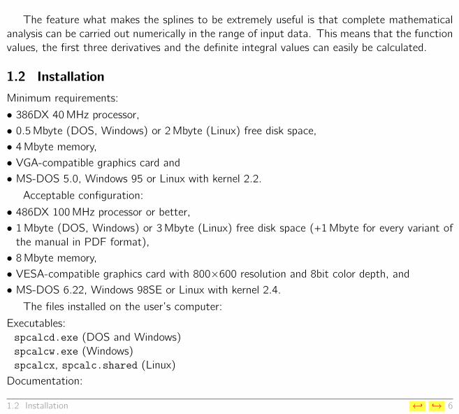
The feature what makes the splines to be extremely useful is that complete mathematicalanalysis can be carried out numerically in the range of input data. This means that the functionvalues, the first three derivatives and the definite integral values can easily be calculated.

1.2 InstallationMinimum requirements:

• 386DX 40MHz processor,• 0.5Mbyte (DOS, Windows) or 2Mbyte (Linux) free disk space,• 4Mbyte memory,• VGA-compatible graphics card and• MS-DOS 5.0, Windows 95 or Linux with kernel 2.2.

Acceptable configuration:

• 486DX 100MHz processor or better,• 1Mbyte (DOS, Windows) or 3Mbyte (Linux) free disk space (+1Mbyte for every variant ofthe manual in PDF format),• 8Mbyte memory,• VESA-compatible graphics card with 800×600 resolution and 8bit color depth, and• MS-DOS 6.22, Windows 98SE or Linux with kernel 2.4.

The files installed on the user’s computer:

Executables:spcalcd.exe (DOS and Windows)spcalcw.exe (Windows)spcalcx, spcalc.shared (Linux)

Documentation:

1.2 Installation ←↩ ↪→ 6

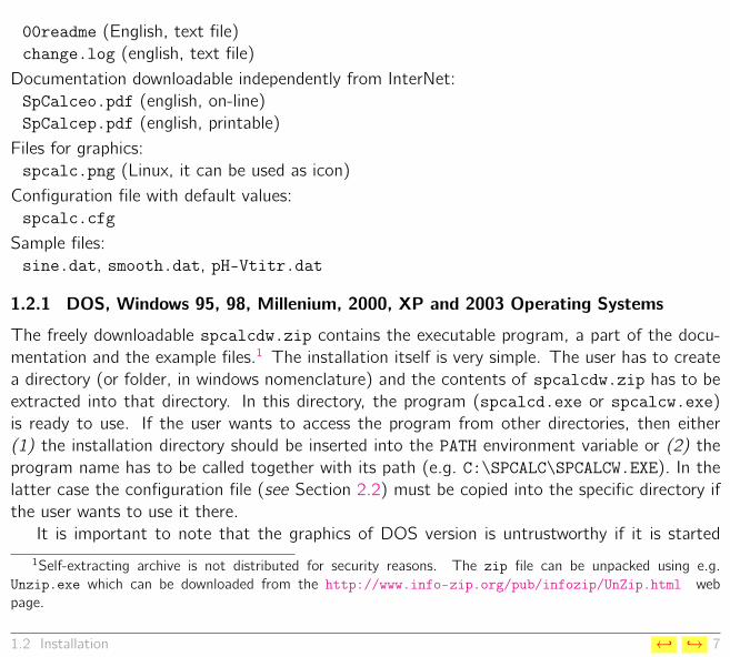
00readme (English, text file)change.log (english, text file)

Documentation downloadable independently from InterNet:SpCalceo.pdf (english, on-line)SpCalcep.pdf (english, printable)

Files for graphics:spcalc.png (Linux, it can be used as icon)

Configuration file with default values:spcalc.cfg

Sample files:sine.dat, smooth.dat, pH-Vtitr.dat

1.2.1 DOS, Windows 95, 98, Millenium, 2000, XP and 2003 Operating Systems

The freely downloadable spcalcdw.zip contains the executable program, a part of the docu-mentation and the example files.1 The installation itself is very simple. The user has to createa directory (or folder, in windows nomenclature) and the contents of spcalcdw.zip has to beextracted into that directory. In this directory, the program (spcalcd.exe or spcalcw.exe)is ready to use. If the user wants to access the program from other directories, then either(1) the installation directory should be inserted into the PATH environment variable or (2) theprogram name has to be called together with its path (e.g. C:\SPCALC\SPCALCW.EXE). In thelatter case the configuration file (see Section 2.2) must be copied into the specific directory ifthe user wants to use it there.

It is important to note that the graphics of DOS version is untrustworthy if it is started1Self-extracting archive is not distributed for security reasons. The zip file can be unpacked using e.g.

Unzip.exe which can be downloaded from the http://www.info-zip.org/pub/infozip/UnZip.html webpage.

1.2 Installation ←↩ ↪→ 7

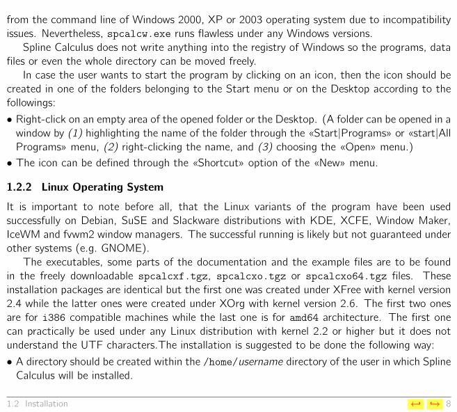
from the command line of Windows 2000, XP or 2003 operating system due to incompatibilityissues. Nevertheless, spcalcw.exe runs flawless under any Windows versions.

Spline Calculus does not write anything into the registry of Windows so the programs, datafiles or even the whole directory can be moved freely.

In case the user wants to start the program by clicking on an icon, then the icon should becreated in one of the folders belonging to the Start menu or on the Desktop according to thefollowings:

• Right-click on an empty area of the opened folder or the Desktop. (A folder can be opened in awindow by (1) highlighting the name of the folder through the «Start|Programs» or «start|AllPrograms» menu, (2) right-clicking the name, and (3) choosing the «Open» menu.)• The icon can be defined through the «Shortcut» option of the «New» menu.

1.2.2 Linux Operating System

It is important to note before all, that the Linux variants of the program have been usedsuccessfully on Debian, SuSE and Slackware distributions with KDE, XCFE, Window Maker,IceWM and fvwm2 window managers. The successful running is likely but not guaranteed underother systems (e.g. GNOME).

The executables, some parts of the documentation and the example files are to be foundin the freely downloadable spcalcxf.tgz, spcalcxo.tgz or spcalcxo64.tgz files. Theseinstallation packages are identical but the first one was created under XFree with kernel version2.4 while the latter ones were created under XOrg with kernel version 2.6. The first two onesare for i386 compatible machines while the last one is for amd64 architecture. The first onecan practically be used under any Linux distribution with kernel 2.2 or higher but it does notunderstand the UTF characters.The installation is suggested to be done the following way:

• A directory should be created within the /home/username directory of the user in which SplineCalculus will be installed.

1.2 Installation ←↩ ↪→ 8

• The file spcalcxf.tgz (or spcalcxo.tgz or spcalcxo64.tgz) has be copied in the previ-ously created directory and extracted with the

tar -xzf spcalcxf.tgz (or spcalcxo.tgz or spcalcxo64.tgz)command.• The file spcalcxf.tgz (or spcalcxo.tgz or spcalcxo64.tgz)can be deleted after extrac-tion.

Certainly there are other means of the installation. If more than one users want to use theprogram and they do not want to have multiple copies of it on the fixed drives then theadministrator (root) may copy the executables to the appropriate directories. The abovedescribed method, however, does not require the help of the system administrator, any user isable to carry out the installation alone.

Two identical executables can be found in each package. The statically linked executable(spcalcx) surely works with any Linux distribution (since it contains everything which is neces-sary during runtime) and this form can be installed and run without the help of the root user, butits size is huge. It may removed if the much smaller dynamically linked one (spcalcx.shared)works. The latter executable, however, depends on many libraries. Essentially, the DISLIN,GRX, tiff, png, jpeg, z and Motif related libraries should be installed to work the dynamicallylinked executable. The exact list of the required shared libraries are the followings:

Under XFree with kernel 2.4 for i386 architecture, the libdislin.so.9, libpng12.so.0,libjpeg.so.62, libtiff.so.4, libgrx20X.so.2, libX11.so.6, libm.so.6,libc.so.6, libpthread.so.0, libXm.so.3, libXt.so.6, libz.so.1, libdl.so.2,/lib/ld-linux.so.2, libXmu.so.6, libSM.so.6, libICE.so.6, libXext.so.6 andlibXp.so.6 libraries must be present.

Under XOrg with kernel 2.6 for i386 architecture the linux-gate.so.1, libdislin.so.9,libpng12.so.0, libjpeg.so.62, libtiff.so.4, libgrx20X.so.2, libX11.so.6,libm.so.6, libc.so.6, libpthread.so.0, libXm.so.4, libXt.so.6, libz.so.1,

1.2 Installation ←↩ ↪→ 9

libXau.so.6, libXdmcp.so.6, libdl.so.2, /lib/ld-linux.so.2, libXmu.so.6,libXext.so.6, libXp.so.6, libXft.so.2, libXrender.so.1, libfontconfig.so.1,libfreetype.so.6, libSM.so.6, libICE.so.6 and libexpat.so.1 libraries must bepresent.

Under XOrg with kernel 2.6 for amd64 architecture the libdislin.so.9, libpng12.so.0,libjpeg.so.62, libtiff.so.4, libgrx20X.so.2, libX11.so.6, libm.so.6,libc.so.6, libpthread.so.0, libXm.so.4, libXt.so.6, libz.so.1, libXau.so.6,libXdmcp.so.6, libdl.so.2, /lib64/ld-linux-x86-64.so.2, libXmu.so.6,libXext.so.6, libXp.so.6, libXft.so.2, libXrender.so.1, libfontconfig.so.1,libfreetype.so.6, libSM.so.6, libICE.so.6 and libexpat.so.1 libraries must bepresent.

After the installation, the programs are ready to use. If the directory of the Spline Cal-culus is listed in the PATH environment variable then the program can be started from an Xterminal window with the spcalcx or spcalcx.shared commands. Otherwise ./spcalcx or./spcalcx.shared commands should be used. The programs can also be started by clickingon an icon. The creation procedure of an icon depends very much on the window manager orgraphical desktop used. The file spcalc.png can be used as the image file of the icon.

There is a third option to use Spline Calculus under Linux. The Windows executable(spcalcw.exe) runs smoothly through WINE.

1.2 Installation ←↩ ↪→ 10

Chapter 2

Using Spline Calculus

The program uses simple text files both for input and output. Additionally, the graphicalrepresentation of the result can also be saved as PNG1 binary image files.

The program reads two files for input: (1) the data file includes the experimental data andoptionally their estimated uncertainties and (2) the configuration file. Four kinds of output filecan be written by the program: (1) the result file includes the coefficients of the interpolatingcubic polynomials and the curves of the graphics display, (2) the user output file containsthe data selected by the user through the graphics display, (3) the message file includes themessages of Spline Calculus during calculations and (4) the image files contain the user selectedgraphics displays.

The configurable options of the program can be set in the following order:

1. Options are set through the command line parameters have the higher precedence.2. Options are set in the configuration file have the next precedence.3. Under Windows and Linux, if the name of the data file is not set either through a command

line parameter or in the configuration file then a file open dialog asks the user to choose thedata file.

4. Options are not set use their default values.1PNG is the abbreviation of Portable Network Graphics. Homepage: http://www.libpng.org/pub/png/ .

←↩ ↪→ 11

2.1 Data FileThe structure of this file is simple as the sample files illustrates. There can be redundantrows at the beginning of the file including titles, descriptions, remark, etc. The rest of thefile contains the input data arranged in columns. At least two columns must exist, the valuesof the independent (x) and dependent (y) data. The column of the deviation values (seeSubsection 2.2.3 in detail) is optional. The sequence of the data must be the same in eachrow.

If a string in the x- or y -column does not represent a real number, the whole row is omitted.If a string in the deviation column cannot be a real number, the default value will be employedfor δ. The x-values must be in increasing sequence downward in the file. If it is not so, theprogram sorts the rows before fitting the spline. If two rows has the same x-value, the programis stopped.

2.2 Configuration FileThe name of the configuration file is supposed to be "spcalc.cfg" initially. The program looksfor this file in the actual directory at first. If it is not found then the name of the executable issupposed for the configuration file. For example, if the name of the program is spcalcw.exethen the spcalcw.cfg file is searched on the actual directory.2 If the actual directory does notcontain any configuration file then the file is searched in the directory where the program isplaced. If no configuration file is found, the default values are used.

In the configuration file, each line sets one option. The only exception is the first one: itmust include the "[SpCalc]" string. If a row includes a hash mark (#) then everything behindthis character (including the hash mark itself) is considered as remark. The file can include

2Another example for Linux: if the name of the executable is spcalcx.shared then the supposed name forthe configuration file is spcalcx.cfg.

2.2 Configuration File ←↩ ↪→ 12

empty lines and remark lines,3 too.An option can be set by the help of the "keyword=value" syntax. There can be space(s)

and/or tab key(s) before and after the "=" sign. Each option must occur after the row including"[SpCalc]" since everything is omitted before this row. The following subsections detail thekeywords4 that can be used

2.2.1 Keywords for the File Names

InputFileName default value: spcalc.dat

The value of this keyword is the name of the data file. The name can also include the fullpath with maximum 255 characters.

OutputFileName default value: spcalc.out

The value of this keyword is the name of the result file. The name can also include the fullpath with maximum 255 characters.

CalcDataFileName default value: spcalc.cal

The value of this keyword is the name of the user output file. The name can also include thefull path with maximum 255 characters.

LogFileName default value: spcalc.log

The value of this keyword is the name of the message file. The name can also include the fullpath with maximum 255 characters.

ImageBaseFileName default value: spcal

The value of this keyword is the first part of the names of the image files. For example, ifthis value is "plot" and an image is to be saved, the program searches for the plot000.png,plot001.png, etc. files until the file does not exist in the actual directory. This non-existentfilename is used for the image file to be saved next.

3In remark lines, the first character is a hash mark.4The keywords are case insensitive.

2.2 Configuration File ←↩ ↪→ 13

2.2.2 Keywords for the Data to be Used

ColumnX default value: 1

The value of this keyword is the number of the column of the independent x-values in thedata file.

ColumnY default value: 2

The value of this keyword is the number of the column of the dependent y -values in the datafile.

OmittedRows default value: 0

The value of this keyword is the number of the rows to be skipped in the beginning of thedata file.

ColumnError default value: 0

The value of this keyword is the number of the column of the relative deviation values (seeSubsection 2.2.3 in detail) in the data file. If the value is zero then default value is used for therelative deviations of the dependent y -values. It should be emphasized that if ColumnError isset (i.e., its value is larger then zero) then the data file must contain at least three columns.

2.2.3 Keywords for the Deviations

Initially, all deviations of y -values (δi) are set to (ymax−ymin)/106 (i.e., one millionth of the y -range). This value is called initial base error. After the initialization, the δi values are multipliedby the relative deviations. The latter values are taken from the column of the data file definedby the keyword "ColumnError". If no column defined for the relative deviations or the definedcolumn contains missing values5 then the default value (1.0) is used for the relative deviations.This default value can be changed by the keyword "ErrorValue". Beside the ColumnError,the following keywords influences the δi values:

5Such string is considered to be a missing value which is not able to represent a real number.

2.2 Configuration File ←↩ ↪→ 14

ErrorValue default value: –1.0

If this value is set to a positive real number then this number becomes the default relativedeviation value. If the value of this keyword is negative then the default relative deviation is1.0.

ErrorRatio default value: no

This keyword should equal to the "no" or should start with the "yes" string (case insensitively).In the latter case, a small positive integer number can follow the "yes" word. If the numberis not indicated it is supposed to be 1.In case of "yes", the deviation values are weighted according to the slope of the curve definedby the x- and y -values. The slope is approximated by linear interpolation. The integer numberdetermines how many neighboring points are used for the linear interpolation both from andfrom right. For example, if the number is 2 then the actual point itself, the two closest pointsfrom left and the two closest points from right are used, so the linear interpolation uses fivesuccessive points all together.

2.2.4 Keywords for Modifying the Outputs

ShowCalculus default value: yes

If this value is set to "yes" the points minimum, the points of maximum and the points ofinflection are indicated on the screen and they are written into the result file. Otherwise, thiskeyword should set to "no" and the result of the mathematical analysis are indicated neitheron the screen nor in the result file.

WriteCurve default value: yes

If this value is set to "yes" the points of the displayed calculated curve are also written intothe result file. These data have fine resolution and they can be used for quick estimation ofthe function values, the first three derivatives and definite integral values. Otherwise, thiskeyword should set to "no" and the result file will not contain the data of the displayedcalculated curve.

2.2 Configuration File ←↩ ↪→ 15

NumberDigits default value: 7

This value determines the precision, i.e. it gives the number of significant digits of the floatingpoint numbers in the result file.

DisplayDigits default value: 5

This value determines the precision, i.e., it gives the number of significant digits of the floatingpoint numbers on the screen.

2.2.5 Keywords for Choosing an Appropriate Graphics Driver

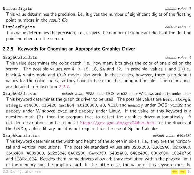
GraphColorBits default value: 4

This value determines the color depth, i.e., how many bits gives the color of one pixel on thescreen. The possible values are 4, 8, 15, 16, 24 and 32. In principle, values 1 and 2 (i.e.,black & white mode and CGA mode) also work. In these cases, however, there is no defaultvalues for the color codes, so they have to be set in the configuration file. The color codesare detailed in Subsection 2.2.7.

GraphGRXDriver default value: VESA under DOS, win32 under Windows and xwin under Linux

This keyword determines the graphics driver to be used. The possible values are herc, stdvga,stdega, et4000, cl5426, mach64, ati28800, s3, VESA and memory under DOS; win32 andmemory under Windows; xwin and memory under Linux. If the value of this keyword is aquestion mark (?) then the program tries to detect the graphics driver automatically. Adetailed description can be found at http://grx.gnu.de/grx246um.htm for the drivers ofthe GRX graphics library but it is not required for the use of Spline Calculus.

GraphResolution default value: 640x480

This keyword determines the width and height of the screen in pixels, i.e., they are the horizon-tal and vertical resolutions. The possible standard values are 320x200, 320x240, 320x400,360x480, 400x300, 512x384, 640x200, 640x350, 640x400, 640x480, 800x600, 1024x768and 1280x1024. Besides them, some drivers allow arbitrary resolution within the physical limitof the memory and the graphics card. In the latter case, the value of this keyword must be

2.2 Configuration File ←↩ ↪→ 16

two integer values (width and height) joined with an "x" without spaces.

These three keywords are not independent of each other, only certain triplets work well.The program is able to detect all correct triplets automatically. The program carries out thisdetection and writes the possible triplets into the message file6 if any of the following conditionsis fulfilled:

• The keyword GraphGRXDriver has an invalid value.• The value of keyword GraphResolution does not correspond to the above rules syntactically.• The given triplet does not correspond to a valid mode of the used graphics card.• The values of the keywords GraphGRXDriver and GraphResolution are question marks.

For example, the programmer’s computer gives the following list of the valid drivers andgraphics modes:

SplineCalculus v2.00a-20060727 has started ...

The required graphic mode cannot be initialized. Supported graphic modes forthe available drivers are (BPP: color depth in bits, Width and Height:horizontal and vertical sizes of the graph given in pixels):

BPP Width Height BPP Width Height BPP Width Height BPP Width Height*** Driver: stdvga ***

1 320x200 1 640x200 1 640x350 1 640x4804 320x200 4 640x200 4 640x350 4 640x4808 320x200 8 320x240 8 320x400 8 360x480

*** Driver: stdega ***1 320x200 1 640x200 1 640x350 4 320x2006In this case, the program is terminated after the detection, and it does not carry out any calculation, of course.

2.2 Configuration File ←↩ ↪→ 17

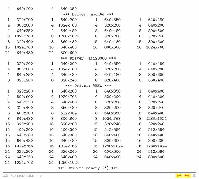
4 640x200 4 640x350*** Driver: mach64 ***

1 320x200 1 640x200 1 640x350 1 640x4804 800x600 4 1024x768 4 320x200 4 640x2004 640x350 4 640x480 8 640x480 8 800x6008 1024x768 8 1280x1024 8 320x200 8 320x2408 320x400 8 360x480 15 640x480 15 800x60015 1024x768 16 640x480 16 800x600 16 1024x76824 640x480 24 800x600

*** Driver: ati28800 ***1 320x200 1 640x200 1 640x350 1 640x4804 800x600 4 1024x768 4 320x200 4 640x2004 640x350 4 640x480 8 640x480 8 800x6008 320x200 8 320x240 8 320x400 8 360x480

*** Driver: VESA ***1 320x200 1 640x200 1 640x350 1 640x4804 800x600 4 1024x768 4 320x200 4 640x2004 640x350 4 640x480 8 320x200 8 320x2408 320x400 8 360x480 8 320x200 8 320x2408 400x300 8 512x384 8 640x350 8 640x4008 640x480 8 800x600 8 1024x768 8 1280x102415 320x200 16 320x200 15 320x240 16 320x24015 400x300 16 400x300 15 512x384 16 512x38415 640x350 16 640x350 15 640x400 16 640x40015 640x480 16 640x480 15 800x600 16 800x60015 1024x768 16 1024x768 15 1280x1024 16 1280x102424 320x200 24 320x240 24 400x300 24 512x38424 640x350 24 640x400 24 640x480 24 800x60024 1024x768 24 1280x1024

*** Driver: memory (!) ***

2.2 Configuration File ←↩ ↪→ 18

1 640x480 4 640x480 8 640x480 24 640x480Behind the driver name, (!) denotes that (besides the standard sizes) thedriver allows to choose arbitrary width and height within the physicallimitation of the graphics adapter and the RAM.

Please, choose valid graphic driver and mode (i.e. correct BPP, width andheight values) in the "SpCalc.cfg" configuration file!

SplineCalculus v2.00a-20060727 has stopped.

Nevertheless, note that the automatic detection is not fool-proof! Sometimes, a triplet isdetected to be valid but it does not work.

2.2.6 Keywords for the Appearance of the Graphics Screen

SizeSymbol default value: 4

The input data are plotted by solid circles on the screen. This value is the radius of the circlesgiven in pixels.

WidthLine default value: 3

The calculated curve is drawn by a solid line on the screen. This value is the width of the linegiven in pixels.

WidthCalculus default value: 1

The results of the mathematical analysis of the calculated curve are nominated on the screenif keyword ShowCalculus is set to yes. The places of the minimums and maximums areindicated by vertical dashed lines and vertical dotted lines indicate the infection points. Thevalue of this keyword is the width of these vertical lines given in pixels.

WidthXplace default value: 1

The focus line shows the actual x-value. The value of this keyword is the width of the focusline given in pixels.

2.2 Configuration File ←↩ ↪→ 19

2.2.7 Keywords for the Display Colors

The colors can be defined by integer numbers. The program uses either an indirect or a directmethod for color definition depending on the color depth.

• The indirect method is used in cases of 1-, 2-, 4- and 8-bit color depth. The colors are storedin a palette, and each color has its own serial number. A specific color can be referenced by itsserial number. The available colors can be displayed by the help of keyword GetColorCodes.In 4- and 8-bit modes, the most frequently used colors (also called VGA-colors) have thefollowing serial numbers:

black: 0 red: 4 dark gray: 8 light red: 12blue: 1 magenta: 5 light blue: 9 light magenta: 13

green: 2 brown: 6 light green: 10 yellow: 14cyan: 3 light gray: 7 light cyan: 11 white: 15

• In cases of 15-, 16-, 24- and 32-bit modes, the direct method is used. It means that theinteger number directly defines the color. An RGB-value7 is used to define a color. Thefollowing binary representations of the integer number and five examples illustrate how the7The RGB-method for the color definition is supposed to be known in this manual. It is described more deeply

at http://grx.gnu.de/grx246um.htm .

2.2 Configuration File ←↩ ↪→ 20

red, green and blue components of the color should be given:

15-bit mode 16-bit mode 24- and 32-bit modebbbbbbbb bbbbbbbb bbbbbbbb bbbbbbbb (bbbbbbbb) bbbbbbbb bbbbbbbb bbbbbbbb︸ ︷︷ ︸

red︸ ︷︷ ︸

green︸ ︷︷ ︸

blue︸ ︷︷ ︸

red︸ ︷︷ ︸

green︸ ︷︷ ︸

blue︸ ︷︷ ︸

red︸ ︷︷ ︸

green︸ ︷︷ ︸

blue

black:x0000000 00000000 00000000 00000000 (xxxxxxxx) 00000000 00000000 00000000

red:x1111100 00000000 11111000 00000000 (xxxxxxxx) 11111111 00000000 00000000

green:x0000011 11100000 00000111 11100000 (xxxxxxxx) 00000000 11111111 00000000

blue:x0000000 00011111 00000000 00011111 (xxxxxxxx) 00000000 00000000 11111111

white:x1111111 11111111 11111111 11111111 (xxxxxxxx) 11111111 11111111 11111111

In 15-bit mode, all the three components are defined by a 5-bit number (0. . .31). In 16-bit mode, the green component is defined by a 6-bit number (0. . .63) while the other twocomponents are still defined by a 5-bit number (0. . .31). In 24- and 32-bit modes, all tehthree components are defined by a byte (0. . .255).

The following keywords can be used to adjust the colors:

ColorBackGround default value: 4-8 bit mode:15; 15 bit mode:32767; 16 bit mode:65535; 24-32 bit

mode:16579836

This value determines the color of the background.ColorText default value: 4-8 bit mode:0; 15 bit mode:0; 16 bit mode:0; 24-32 bit mode: 0

2.2 Configuration File ←↩ ↪→ 21

The color determined by this keyword is used for the regular texts and for the frames on thegraphics screen.

ColorSymbol default value: 4-8 bit mode:4; 15 bit mode:21504; 16 bit mode:43008; 24-32 bit mode: 11010048

This color is used for the solid circles of the input data.ColorLine default value: 4-8 bit mode:1; 15 bit mode:21; 16 bit mode:21; 24-32 bit mode: 168

This color is used for the solid line of the calculated curve.ColorCalculus default value: 4-8 bit mode:8; 15 bit mode:10570; 16 bit mode:21130; 24-32 bit mode: 5526612

This color is used for the dashed and dotted vertical lines nominating the extrema and thepoints of inflection.

ColorXplace default value: 4-8 bit mode:5; 15 bit mode:21525; 16 bit mode:43029; 24-32 bit mode: 11010216

This color is used for the focus line nominating the actual x-value.ColorKeys default value: 4-8 bit mode:12; 15 bit mode:32074; 16 bit mode:64170; 24-32 bit mode: 16536656

This color is used for the shortcut keyns operating on the graphics screen.GetColorCodes default value: no

In 4- and 8-bit mode, if this keyword is set to "yes" then the colors of the actual palette aredisplayed and pressing any key terminates the program.

2.2.8 Other Keywords

JumpSize default value: 1

This value determines the unit of the movement in pixels if the focus line (i.e., the actualx-value) is changed.

SizingStep default value: 0.04

If the user changes the x- and/or y -ranges, this value determines the extent of this change.The value is interpreted as a relative ratio, i.e., 0.04 means that the range is increased (ordecreased) by 4%.

MaxIteration default value: 1000

2.2 Configuration File ←↩ ↪→ 22

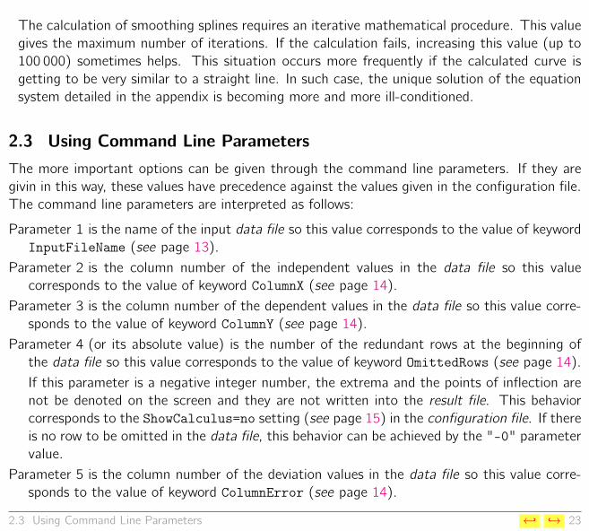
The calculation of smoothing splines requires an iterative mathematical procedure. This valuegives the maximum number of iterations. If the calculation fails, increasing this value (up to100 000) sometimes helps. This situation occurs more frequently if the calculated curve isgetting to be very similar to a straight line. In such case, the unique solution of the equationsystem detailed in the appendix is becoming more and more ill-conditioned.

2.3 Using Command Line ParametersThe more important options can be given through the command line parameters. If they aregivin in this way, these values have precedence against the values given in the configuration file.The command line parameters are interpreted as follows:

Parameter 1 is the name of the input data file so this value corresponds to the value of keywordInputFileName (see page 13).

Parameter 2 is the column number of the independent values in the data file so this valuecorresponds to the value of keyword ColumnX (see page 14).

Parameter 3 is the column number of the dependent values in the data file so this value corre-sponds to the value of keyword ColumnY (see page 14).

Parameter 4 (or its absolute value) is the number of the redundant rows at the beginning ofthe data file so this value corresponds to the value of keyword OmittedRows (see page 14).If this parameter is a negative integer number, the extrema and the points of inflection arenot be denoted on the screen and they are not written into the result file. This behaviorcorresponds to the ShowCalculus=no setting (see page 15) in the configuration file. If thereis no row to be omitted in the data file, this behavior can be achieved by the "-0" parametervalue.

Parameter 5 is the column number of the deviation values in the data file so this value corre-sponds to the value of keyword ColumnError (see page 14).

2.3 Using Command Line Parameters ←↩ ↪→ 23

Parameter 6 corresponds to the integer number given in keyword ErrorRatio. See page 15 forthe interpretation of this number.

2.4 Operating on the Graphics ScreenIf the calculation of the smoothing spline is ended, the program plots the results on the screen(see Figure 2.1 as an example). The displayed window consists of two parts. The upper, framedone shows the results graphically. The lower part include some actual numerical informationand it enumerates the shortcut keys for operating on the screen. The nominations on the graphare the followings:

• The input data are denoted by solid circles.• The calculated smoothing spline is drawn by a solid line. The points of this curve is calcu-lated at 200 or more x-values, depending on the actual slope. These calculated points areconnected.• The extrema are denoted by vertical dashed lines. The line is below the calculated curve ata minimum and it is above the curve at a maximum. If both the first and second derivativesare zero, the dashed line fills the whole displayed y -range.• The points of inflection are denoted by vertical dotted lines. The line below the calculatedcurve means that the values of the third derivative is negative while a line is drawn above thecalculated curve in case of positive third derivative.• If keyword ShowCalculus is set to "no", the extrema and the points of inflection will not bedenoted on the figure.• A vertical solid line denotes the focus line which is always drawn at the actual x-value.Immediately below the graph, some results are displayed: the function value, the first threederivative and the definite integral are written at the actual x-value. Pressing the left buttonof the mouse on the area of the figure changes the actual x-value and moves the focus line

2.4 Operating on the Graphics Screen ←↩ ↪→ 24

to the clicked x-position.

The lower part consists of two rows. The left part of the first one gives two values: (1)the actual value of the base error (see the first paragraph of Subsection 2.2.3) and the averagedeviation from the last calculation. The latter one is the average of the absolute values ofthe differences between the input and calculated y -values, i.e.,

∑ni=1

∣∣y calci − y input

i

∣∣ using thenominations given in the appendix.

The right part of the first row displays the actual position of the mouse in parentheses.The second row of the lower part gives the shortcut keys. They have unique color defined

by keyword ColorKeys. Their actions can be achieved either by pressing the appropriate key orby left-clicking the name of the key with the mouse. The meaning of the shortcut keys are thefollowing:

left , right , up and down denotes the arrows. They move the graph to the correspondingdirection without resizing. The extent of this movement can be set by keyword SizingStep(see page 22).

F1 and F2 decreases and increases the actual x-value, respectively. The focus line followsthe actual x-value. The extent of this change is one pixel by default but it can be modifiedby keyword Jumpsize (see page 22). A more flexible change of the actual x-value is possiblethrough the left button of the mouse.

F3 writes the actual x-value itself, its function value, the first three derivatives and the definiteintegral at the actual x-value into the user output file. Each pressing of this key adds onenew row to the file but restarting the program erases the existing user output file.

F4 saves the current graph into an image file using Portable Network Graphics format. Theimage includes the upper part of the screen, the base error and the average deviation valuesbut it does not contain the current mouse position and the list of the shortcut keys. Thename of the image file is automatically chosen by the program as it is described at keywordImageBaseFileName (see page 13).

2.4 Operating on the Graphics Screen ←↩ ↪→ 25

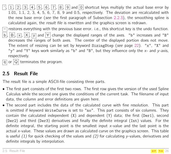
‘ , 1 , 2 , 3 , 4 , 5 , 6 , 7 , 8 , 9 and 0 shortcut keys multiply the actual base error by1.01, 1.1, 2, 3, 4, 5, 6, 7, 8, 9 and 0.5, respectively. The deviation are recalculated withthe new base error (see the first paragraph of Subsection 2.2.3), the smoothing spline iscalculated again, the result file is rewritten and the graphics screen is redrawn.

– restores everything with the previous base error. i.e., this shortcut key is the undo function.

b , B , x , X , y and Y change the displayed ranges of the axes. "b" increases and "B"decreases the ranges of both axes. The center of the displayed portion does not move.The extent of resizing can be set by keyword SizingStep (see page 22). "x", "X" and"y" and "Y" keys work similarly as "b" and "B", but they influence only the x- and y -axis,respectively.

q or Q terminates the program.

2.5 Result FileThe result file is a simple ASCII-file consisting three parts.

• The first part consists of the first two rows. The first row gives the version of the used SplineCalculus while the second one gives the conditions of the current task. The filename of inputdata, the column and error definitions are given here.• The second part includes the data of the calculated curve with fine resolution. This partis omitted if keyword WriteCurve is set to "no". This part consists of six columns. Theycontain the calculated independent (X) and dependent (Y) data; the first (Der1), second(Der2) and third (Der3) derivatives and finally the definite integral (Int) values. For thedefinite integral, the starting point is the smallest input x-value and the last point is theactual x-value. These values are drawn as calculated curve on the graphics screen. This tableis useful (1) for quick checking of the values and (2) for calculating y -values, derivatives anddefinite integrals by interpolation.

2.5 Result File ←↩ ↪→ 26

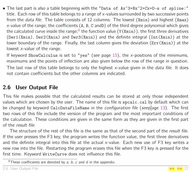
• The last part is also a table beginning with the "Data of Axˆ3+Bxˆ2+Cx+D-s of spline:"title. Each row of this table belongs to a range of x-values surrounded by two successive pointsfrom the data file. The table consists of 12 columns: The lowest (Xmin) and highest (Xmax)x-value of the range; the coefficients (A, B, C andD) of the third degree polynomial which givesthe calculated curve inside the range;8 the function value (Y(Xmin)), the first three derivatives(Der1(Xmin), Der2(Xmin) and Der3(Xmin)) and the definite integral (Int(Xmin)) at thelower boundary of the range. Finally, the last column gives the deviation (Err(Xmin)) at thelowest x-value of the range.If keyword ShowCalculus is set to "yes" (see page 15), the x-positions of the minimums,maximums and the points of inflection are also given below the row of the range in question.The last row of this table belongs to only the highest x-value given in the data file. It doesnot contain coefficients but the other columns are indicated.

2.6 User Output FileThis file makes possible that the calculated results can be stored at only those independentvalues which are chosen by the user. The name of this file is spcalc.cal by default which canbe changed by keyword CalcDataFileName in the configuration file (seep]age 13). The firsttwo rows of this file include the version of the program and the most important conditions ofthe calculation. These conditions are given in the same form as they are given in the first partof the result file.

The structure of the rest of this file is the same as that of the second part of the result file.If the user presses the F3 key, the program writes the function value, the first three derivativesand the definite integral into this file at the actual x-value. Each new use of F3 key writes anew row into the file. Restarting the program erases this file when the F3 key is pressed for thefirst time. Keyword WriteCurve does not influence this file.

8These coefficients are denoted by a, b, c and d in the appendix.

2.6 User Output File ←↩ ↪→ 27

2.7 Message FileThis file contains the runtime messages and error descriptions. The old version of this file isalways erased at the start of the program. In case of automatic graphics driver and graphicsmode detection (see Subsection 2.2.5) the message file includes the available drivers and theirmodes.

2.7 Message File ←↩ ↪→ 28

Figure 2.1: The graphics screen of the program.

2.7 Message File ←↩ ↪→ 29

AppendixMathematical Background

Given a set of (xi , yi) (i = 1 . . . n) data pairs where xj 6= xk (j = 1 . . . n, k = 1 . . . n), i.e.,duplicated independent values are not allowed. Supposing that xi values are sorted in increasingorder, the aim of any interpolating procedure is to estimate the dependent y -values at any x inthe [x1, xn] interval.

Using splines is one possibility for the interpolation. It can be proved mathematically thatthe natural cubic spline is the smoothest interpolating curve which means that this curve hasthe smallest ∫ xn

x1

(f ′′(x))2 dx

value for a specific data set.

Natural Cubic Spline

This expression means that a cubic polynomial (y=a·x3+b·x2+c ·x+d) is used to connect twosuccessive points. Figure 2 illustrates the natural cubic splines. Since the [x1, xn] interval aredivided into (n−1) ranges by the x2, . . . , xn−1 values, 4·(n−1) coefficients should be calculated(they are the ai , bi , ci and di (i = 1 . . . n−1) values). This can be done by applying the followingrestrictions and assumptions:

←↩ ↪→ 30

x1 x2 · · · xi xi+1 · · · xn−1 xn

y1

y2

...

yi , yi+1

...

yn−1, yn

natural cubic spline

smoothing spline

y =

a1·x3+b1·x2+c1·x +d1

y =

ai·x3+bi·x2+ci·x +di

y =

an−1·x3+bn−1·x2+cn−1·x +dn−1

Figure 2: Illustration for the splines and the used notations.

• The function values at the inner endpoints of the ranges can be calculated from any of theneighboring cubic polynomials:

yi = ai · x3i + bi · x2i + ci · xi + di (i = 1 . . . n − 1) and

yi = ai−1 · x3i + bi−1 · x2i + ci−1 · xi + di−1 (i = 2 . . . n) .(1)

It also means that the overall interpolating function is continuous. The left and right limits ofthe function values are the same, so there is no point of discontinuity in the [x1, xn] interval.

Appendix ←↩ ↪→ 31

• The left and right limits of the values of the first derivative should be the same at the innerendpoints of the used interval:

3ai · x2i + 2bi · xi + ci = 3ai+1 · x2i + 2bi+1 · xi + ci+1 (i = 2 . . . n−1) . (2)

As a consequence of this equation, there is no break point inside the [x1, xn] interval.• The left and right limits of the values of the second derivative should be the same at the innerendpoints of the used interval:

6ai · xi + 2bi = 6ai+1 · xi + 2bi+1 (i = 2 . . . n−1) . (3)

• Finally, two restrictions must be set to the second derivative at the endpoints of the overallinterval:

6a1 · x1 + 2b1 = 0 and 6an−1 · xn + 2bn−1 = 0 , (4)

i.e., there are points of inflection at both ends of the overall interval.

Equations (1–4) forms an exact linear equation system (the number of equations is the sameas the number of parameters to be determined), so the coefficients of the cubic polynomials canunambiguously be determined. With these coefficients, the function values, the first, secondand third derivatives and the definite integrals can be calculated.

Smoothing SplineSmoothing spline is a modified case of the natural cubic spline. The smoothing spline does notgo through the (xi , yi) (i = 1 . . . n) data points, it just appropriately nears to them around theirdeviations (δi) as it can be seen in Figure 2. It means mathematically that the

n−1∑i=1

(yi − ai · x3i − bi · x2i − ci · xi − di

δi

)2+

(yn − an−1 · x3n − bn−1 · x2n − cn−1 · xn − dn−1

δn

)2n

≤ 1Appendix ←↩ ↪→ 32

inequality must also be fulfilled together with Equations (2–4) and with the following equations:

ai−1 · x3i + bi−1 · x2i + ci−1 · xi + di−1 = ai · x3i + bi · x2i + ci · xi + di (i = 2 . . . n−1)

This equation system usually has unique solution for ai , bi , ci and di (i = 1 . . . n−1) at reasonablysmall δi values. However, if the δi values are large then infinite number of lines (the regressionline is also among them) can be the solution.

It should be emphasized that the δi values are constant input data together with the xi andyi ones. They are not minimized during the calculation of the coefficients since the splines arenot related to the non-linear parameter estimating procedures in any way.

Appendix ←↩ ↪→ 33