Use of correspondence analysis in clustering a mixed-scale ...

Economics Working Paper Series

Working Paper No. 1626

Use of correspondence analysis in clustering a mixed-scale data set with

missing data

Michael Greenacre

January 2019

Use of Correspondence Analysis in Clustering aMixed-Scale Data Set with Missing Data

Michael Greenacre

Abstract Correspondence analysis is a method of dimension reduction for cat-egorical data, providing many tools that can handle complex data sets. Obser-vations on different measurement scales can be coded to be analysed togetherand missing data can also be handled in the categorical framework. In thisstudy, the method’s ability to cope with these problematic issues is illustrated,showing how a valid continuous sample space for a cluster analysis can beconstructed from the complex data set from the IFCS 2017 Cluster Challenge.

1 Introduction

This short article details my approach to the clustering of 928 lower back painpatients using the dataset of self-reported baseline assessments from the IFCSCluster Challenge in 2017. Since the majority of the data are categorical, I havetaken the route of correspondence analysis and related methods (CARME) toarrive at a solution, in the process making use of multiple correspondence anal-ysis, subset correspondence analysis, fuzzy coding, and k-means clustering inreduced-dimensional space. In the course of the methodological description, Ipoint out the benefits and drawbacks of each step of the process. For the mostpart, the drawbacks can give rise to interesting problems as side-issues, whichare suitable for masters-level projects.

Michael GreenacreUniversitat Pompeu Fabra, Ramon Trias Fargas 25–27, Barcelona.� [email protected]

ISSNVol. , No. ,

2 Michael Greenacre

2 The data and data recoding

The data for each of the 928 patients consists of 112 variables, whose descrip-tions are further detailed in this special issue by ?. For the statistical treatment,the variables fall into the following categories (numbers of variables in eachcase):

Continuous 8Dichotomous 64

Multistate Nominal 9Ordinal 30

Trichotomous 1

To reduce all data to a categorical scale, the eight continuous variables werefuzzy coded (?) into four fuzzy categories plus a missing value category. Thisis a generalization of dummy variable, or “crisp”, coding. Instead of cuttingup the range of the continuous variable into intervals and coding a particularvalue strictly into one of the intervals, the value is coded in a fuzzy way intoadjacent intervals.

For example, a value might be coded into the five-category variable as[ 0 0.15 0.85 0 0 ] to show that it is 15% in fuzzy category 2 and 85%in fuzzy category 3. A missing value would be coded as [ 0 0 0 0 1 ]. Hence,for each continuous observation, this coding produces four values between 0and 1 (inclusive), summing to 1, precisely coding the continuous value in thefour categories, and a missing value in the fifth. The fuzzy values are deter-mined from a continuous value using a set of membership functions — for adetailed description, see ? or ?, chapter 3

The only variable that presented a problem with this coding was obeh0,which has 333 values of 0 (i.e. 333 respondents completely agree that treatmentis necessary to decrease their pain), so this variable was coded into a crispcategory for the zeros, and 3 fuzzy categories for the other positive values.The other 104 categorical variables generated small numbers of categories, thecounts of each of which are as follows:

Variables with 2 categories 64



Use of Correspondence Analysis in Clustering 3





These were all treated as nominal for the subsequent correspondence analysis(CA) approach, even though many of them (30) are ordinal. Notice that foreach variable that has missing values, a separate code (in this case a "9" wasused) for missing values and thus a separate category. Since our methodologywill be purely nominal, combined with the fuzzy categories, the missing valuecategories are just additional categories of the data set.

Benefits : All variables are reduced to the same measurement scale.The fuzzy coding especially is useful to categorize continuous vari-ables without losing information (the fuzzy-coded variables can be back-transformed to their original continuous values) and also allow nonlinearinter-relationships to be taken into account. The missing value problemis obviated by the simple addition of missing value categories where nec-essary for the corresponding variables.

Drawbacks : The ordinal information in the 30 ordinal variables is lost.For ordinal variables with many categories, e.g. those with 7 and 8 cate-gories, a fuzzy coding could have been contemplated. On the other hand,a completely different approach, based on Gower’s mixed-scale distancefunction could be used (?), implemented in the R package cluster, forexample.

3 Methods

3.1 Step 1 – Subset multiple correspondence analysis

Multiple correspondence analysis (MCA) is the analogue of principal compo-nent analysis (PCA) for multivariate categorical data, leading to optimal quan-tifications of the categories and a multivariate Euclidean space of the individ-uals. The number of categories is 430, consisting of dummy variables for thecategorical variables, fuzzy categories for the continuous variables and missing

4 Michael Greenacre

value categories where necessary. The inclusion of missing value categoriesinvariably leads to them dominating the solution, because of their strong asso-ciations in the responses. This would be fine if the idea were to study patternsof missing values, but in the present case respondent groups are required basedon substantive answers to the survey, not on the pattern of missing responses.

A variant of MCA called subset MCA, where certain chosen categories canbe suppressed, is designed for this situation, described by ??. In the subsetversion, missing value categories are not omitted in the original matrix butrather in the matrix of respondent profiles, which are the rows of the crisp andfuzzy values of the dummy variables divided by their respective totals. Thenthe usual chi-square normalization inherent in correspondence analysis andthe dimension reduction calculations are performed on the retained columns— see ?, chapter 21 for further examples. Hence, in this step, subset MCA isperformed, declaring the missing value categories out of the subset.

3.2 Step 2 – Choice of dimensionality

Whereas the number of categories in the recoded data is 430, the actual num-ber of dimensions of this analysis is 309, due to the many linear relationships,one for each categorical variable, and several missing categories being out ofthe subset. The rule for determining the number of “true” dimensions in a reg-ular MCA is applied here and we remove all dimensions below the eigenvaluethreshold of 1/Q where Q = number of variables, i.e. 1/112. 1 This rule sug-gests that the dimensionality is 73, so in the following the first 73 dimensionsare used, which situates all the respondents in a 73-dimensional continuousEuclidean space, which can be handled by standard methods.

3.3 Step 3 – Clustering using k-means

Nonhierarchical k-means clustering is performed in the 73-dimensional spaceobtained above. To determine the number of clusters, the clustering is per-formed for 2, 3, 4, ..., 15 clusters, each repeated with one of 50 random startingpoints, and up to 500 iterations maximum. The improvement in the between-

1 See ?, chapter 19 and the conjecture on the last page of this book that the true dimensionalityof a multivariate categorical data matrix is determined by this rule. This conjecture is based on theidea that the dimensionality of a categorical data set is the number of dimensions required to fit allpairwise cross-tabulations exactly in a joint correspondence analysis (JCA), which holds true forsimple correspondence analysis.


cluster sum-of-squares is used to decide on the number of clusters, similar tothe scree plot in PCA, making use of the elbow “rule-of-thumb”.

3.4 Step 4 – Cluster interpretation using correspondence analysis

The clusters are interpreted by cross-tabulating them with all the variables,and performing a correspondence analysis on this concatenated table. This ta-ble has the clusters as column categories and the rows as all the categories ofthe variables used to establish the clusters. ? call this a CA centroid discrimi-nant analysis, which is in fact a variation of canonical correspondence analysis(CCA) (?), where the constraining variable is the set of dummies (i.e. crispcategorical variables) for the clusters. (If fuzzy clustering is performed, thefuzzy coded memberships can be similarly used.) The variables that make thehighest contributions to separating the clusters are identified in an ordered listand provide an indication of the cluster characteristics.

Benefits : The coding and the MCA have brought the whole data set intoEuclidean space, and thus the remainder of the exercise is traightforward.The subset idea is put to good use here, and allows all respondents tobe used without the inevitable associations amongst the missing valuecategories, which interfere with the results.

Drawbacks : The conjecture about the true dimensionality of the dataset was used. But the conjecture has so far stood up to empirical jus-tification, and no convincing counterexample has been found. Also, thedata matrix was not of “pure” categorical data, with dummy variables allcrisply coded, but contained 8 fuzzy-coded variables — this is an aspectworth following up.

4 Results

Having extracted the first 73 dimensions of the recoded data set in the subsetMCA of the crisp- and fuzzy-coded variables, the k-means clustering gavethe following results (Fig. 1). From seven clusters onwards the improvementsare small and tailing off, so the six-cluster solution is preferred, with 42.5%

6 Michael Greenacre

Fig. 1 On the left, thebetween-cluster sum ofsquares (BSS) relative tototal sum of squares (TSS)for increasing number of clus-ters (starting from one clusterwhere BSS=0). On the right,the increment (improvement),starting from the benefit fromtwo to three clusters. Thesix-cluster solution is chosen.

3

discriminant analysis, in fact it is a variation of canonical correspondence analysis, CCA (ter

Braak, 1986) where the constraining variable is the set of dummies for the clusters. The

variables that make the highest contributions to separating the clusters are identified in an

ordered list and provide an indication of the cluster characteristics.

Benefits: The coding and the MCA has brought the whole data set into Euclidean space, and

thus the remainder of the exercise is pretty straightforward. The subset idea is put to good

use here, and allows all respondents to be used without the inevitable associations amongst

the missing value categories to interfere with the results.

Drawbacks: The conjecture about the true dimensionality of the data set1 was used. But the

conjecture has pretty much stood up to empirical justification so far, and no clear

counterexample has been found. Also, the data matrix was not of "pure" categorical data,

with dummy variables all crisply coded, but contained 8 fuzzy‐coded variables this aspect is interesting to follow up.

4 Results

Having extracted the first 73 dimensions of the recoded data set in the subset MCA (with the

variation that the continuous variables are fuzzy‐coded), the k‐means clustering gave the

following results (Figure 1).

Figure 1: On the left, the between‐cluster sum of squares (BSS) relative to total sum of squares (TSS) for increasing number of clusters (starting from 1 cluster, BSS=0). On the right, the increment (improvement), starting from the benefit from 2 to 3 clusters. From 7 onwards the improvements are small and tailing off, so the 6‐cluster solution is preferred.

1 The conjectured definition of the dimensionality is a generalization of the definition for simple correspondence analysis, namely it is the number of dimensions required to fit all pairwise cross‐tabulations exactly in a joint correspondence analysis (JCA), where JCA optimizes fit to the off‐diagonal tables of the Burt matrix, ignoring the diagonal matrices down the block diagonal. See Greenacre (2016a, last page of book).

2 4 6 8 10 12 14

0.0

0.1

0.2

0.3

0.4

0.5

Number of clustersB

SS

/TS

S2 4 6 8 10 12 14

0.02

0.04

0.06

0.08

Nr of clusters

imp

rov

em

en

t

of the total variance explained by between-cluster variance. The number ofrespondents in each cluster are as follows:

Cluster 1 Cluster 2 Cluster 3 Cluster 4 Cluster 5 Cluster 690 189 191 177 47 234

For interpretation of the clusters, the CA of the six clusters cross-tabulated withall 112 variables yields an analysis with five dimensions, and the followingeigenvalues (output from R package ca by ? reported here):

dim value % cum% scree plot1 0.093964 56.8 56.8 **************2 0.033384 20.2 76.9 *****3 0.022624 13.7 90.6 ***4 0.009153 5.5 96.1 *5 0.006378 3.9 100.0 *

-------- -----Total: 0.165503 100.0

Using the "elbow" rule of thumb (which is essentially what was used in Fig. 1,on the right, to decide on the number of clusters), it seems that the result isthree-dimensional, with 9.4% of the inertia that can be ascribed to randomfluctuations.

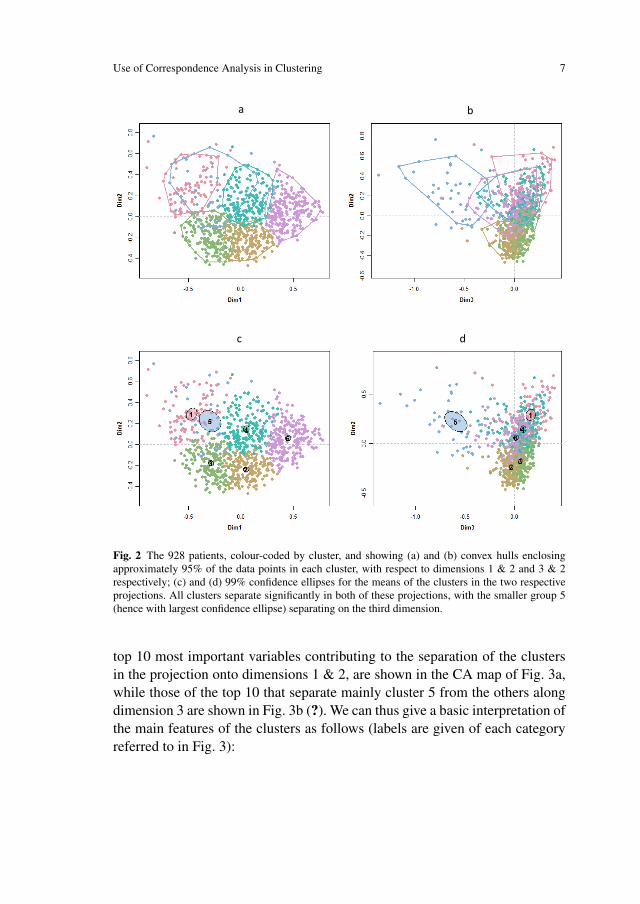
Fig. 2 shows the CA maps of the respondents, coloured according to theircorresponding clusters, in dimensions 1 and 2, and then rotated around thesecond axis to show dimensions 3 and 2. In Figs 2a and 2b the peeled convexhulls, enclosing approximately 95% of the points in each cluster are shown,with respect to the two planar projections. In Figs 2c and 2d, the 99% con-fidence ellipses for the means of each cluster are shown. As supplementarymaterial an animation is given in a GIF file (see ? for example, for a descrip-tion of the meaning of these ellipses and 3D ellipsoids).The categories of the


Figure 2: The 928 patients, colour‐coded by cluster, and showing (a) and (b) convex hulls enclosing approximately 95% of the data points in each cluster, with respect to dimensions 1 & 2 and 3 & 2 respectively; (c) and (d) 99% confidence ellipses for the means of the clusters in the two respective projections. All clusters separate significantly in both of these projections, with the smaller group 5 (hence with largest confidence ellipse) separating on the third dimension.

a b

c d

Fig. 2 The 928 patients, colour-coded by cluster, and showing (a) and (b) convex hulls enclosingapproximately 95% of the data points in each cluster, with respect to dimensions 1 & 2 and 3 & 2respectively; (c) and (d) 99% confidence ellipses for the means of the clusters in the two respectiveprojections. All clusters separate significantly in both of these projections, with the smaller group 5(hence with largest confidence ellipse) separating on the third dimension.

top 10 most important variables contributing to the separation of the clustersin the projection onto dimensions 1 & 2, are shown in the CA map of Fig. 3a,while those of the top 10 that separate mainly cluster 5 from the others alongdimension 3 are shown in Fig. 3b (?). We can thus give a basic interpretation ofthe main features of the clusters as follows (labels are given of each categoryreferred to in Fig. 3):

8 Michael Greenacre6

Figure 3: (a) The 10 most important contributors to the two dimensional CA solution that separates the clusters; (b) the 10 most important contributors to the separation of cluster 5 on the third axis.

a

b

Fig. 3 (a) The 10 most important contributors to the two dimensional CA solution that separates theclusters; (b) the 10 most important contributors to the separation of cluster 5 on the third axis.


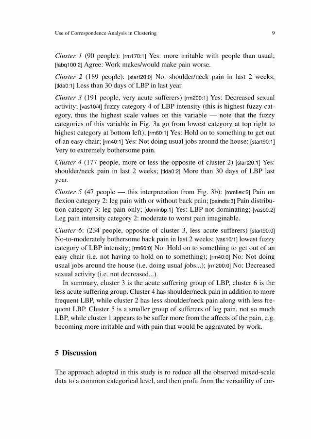
Cluster 1 (90 people): [rm170:1] Yes: more irritable with people than usual;[fabq100:2] Agree: Work makes/would make pain worse.

Cluster 2 (189 people): [start20:0] No: shoulder/neck pain in last 2 weeks;[tlda0:1] Less than 30 days of LBP in last year.

Cluster 3 (191 people, very acute sufferers) [rm200:1] Yes: Decreased sexualactivity; [vas10/4] fuzzy category 4 of LBP intensity (this is highest fuzzy cat-egory, thus the highest scale values on this variable — note that the fuzzycategories of this variable in Fig. 3a go from lowest category at top right tohighest category at bottom left); [rm60:1] Yes: Hold on to something to get outof an easy chair; [rm40:1] Yes: Not doing usual jobs around the house; [start90:1]

Very to extremely bothersome pain.

Cluster 4 (177 people, more or less the opposite of cluster 2) [start20:1] Yes:shoulder/neck pain in last 2 weeks; [tlda0:2] More than 30 days of LBP lastyear.

Cluster 5 (47 people — this interpretation from Fig. 3b): [romflex:2] Pain onflexion category 2: leg pain with or without back pain; [paindis:3] Pain distribu-tion category 3: leg pain only; [dominbp:1] Yes: LBP not dominating; [vasb0:2]

Leg pain intensity category 2: moderate to worst pain imaginable.

Cluster 6: (234 people, opposite of cluster 3, less acute sufferers) [start90:0]

No-to-moderately bothersome back pain in last 2 weeks; [vas10/1] lowest fuzzycategory of LBP intensity; [rm60:0] No: Hold on to something to get out of aneasy chair (i.e. not having to hold on to something); [rm40:0] No: Not doingusual jobs around the house (i.e. doing usual jobs...); [rm200:0] No: Decreasedsexual activity (i.e. not decreased...).

In summary, cluster 3 is the acute suffering group of LBP, cluster 6 is theless acute suffering group. Cluster 4 has shoulder/neck pain in addition to morefrequent LBP, while cluster 2 has less shoulder/neck pain along with less fre-quent LBP. Cluster 5 is a smaller group of sufferers of leg pain, not so muchLBP, while cluster 1 appears to be suffer more from the affects of the pain, e.g.becoming more irritable and with pain that would be aggravated by work.

5 Discussion

The approach adopted in this study is ro reduce all the observed mixed-scaledata to a common categorical level, and then profit from the versatility of cor-

10 Michael Greenacre

respondence analysis in quantifying multivariate categorical data and bringingthe data set into a valid continuous space. Once the samples are embeddedin this space, an algorithm such as k-means clustering can be implemented ina standard way. The clusters that have been revealed by this approach havea substantive interpretation in terms of the variables that are determinant indefining the clusters. Moreover, this interpretation is facilitated by using cor-respondence analysis again in the final stage, in order to map the revealedclusters and the categorical variables. Thus, correspondence analysis assists inboth analysing the data and analysing the results, which are themselves quitecomplex, composed of six clusters constructed from over 112 variables codedinto a total of 430 categories.

Supplementary material

A Flash animation (.swf format) shows the rotation of the individuals andcluster confidence ellipsoids in three-dimensional space.A video presentation of this article can be found at the CARMEnetworkYouTube channel (CARME = Correspondence Analysis and Related Methods),https://www.youtube.com/CARMEnetwork. The video includes someadditional results, comparing the clusters according to the demographical vari-ables sex and age, as well as according to the three longitudinal outcomesobserved during the one-year period after these survey data were collected:global perceived improvement, LBP intensity and Roland-Morris score.There are two small errata in the video. On a summary slide of the clusters,at time 8:50, cluster 1 at the top left is erroneously labelled cluster 2. Further-more, the interpretation of clusters 2 and 4 suffers from a data coding problemwhich was only recently discovered in the supplied data file. The descriptionof these clusters has been corrected in the present article.

https://www.youtube.com/CARMEnetwork


References

Asan Z, Greenacre M (2011) Biplots of fuzzy coded data. Fuzzy Sets andSystems 183:57–71

Gower J (1971) A general coefficient of similarity and some of its properties.Biometrics 27:857–871

Greenacre M (2013) Contribution biplots. Journal of Computational andGraphical Statistics 22:107–122

Greenacre M (2016a) Correspondence Analysis in Practice. Chapman &Hall/CRC

Greenacre M (2016b) Data reporting and visualization in ecology. Polar Biol-ogy 39:2189–2205

Greenacre M, Pardo R (2006a) Multiple correspondence analysis of subsets ofresponse categories. In: Greenacre M, Blasius J (eds) Multiple Correspon-dence Analysis and Related Methods, Chapman & Hall/CRC, Boca Raton,FL, pp 197–217

Greenacre M, Pardo R (2006b) Subset correspondence analysis: visualizationof selected response categories in a questionnaire survey. Sociological Meth-ods and Research 35:193–218

Greenacre M, Primicerio R (2013) Multivariate Analysis of Ecological Data.BBVA Foundation, Bilbao, Spain

Nenadic O, Greenacre M (2006) Correspondence analysis in R, with two- andthree-dimensional graphics: the ca package. Journal of Statistical Software20, URL http://www.jstatsoft.org/v20/i03

Ter Braak C (1986) Canonical correspondence analysis: a new eigenvectortechnique for multivariate direct gradient analysis. Ecology 67:1167–1179

Van Mechelen I, Vach W (2018) Cluster analyses of a target data set in theifcs cluster benchmark data repository: Introduction to the special issue.Archives of Data Science 10:1–16

http://www.jstatsoft.org/v20/i03

Use of correspondence analysis in clustering a mixed-scale ...

Documents

Transcript of Use of correspondence analysis in clustering a mixed-scale ...