
U.S.DEPARTMENT OF ENERGY - smart grid · PDF fileU.S.DEPARTMENT OF ENERGY ... usefulness of...
102
Submitted To: U.S.DEPARTMENT OF ENERGY BORREGO SPRINGS MICROGRID DEMONSTRATION PROJECT DOE Award No: DE-FC26-08NT02870 Final Technical Report Submitted By: San Diego Gas & Electric Date Submitted: September, 2014
-
Upload
trinhtuyen -
Category
Documents
-
view
214 -
download
0
Transcript of U.S.DEPARTMENT OF ENERGY - smart grid · PDF fileU.S.DEPARTMENT OF ENERGY ... usefulness of...

Submitted To:
U.S.DEPARTMENT OF ENERGY
BORREGO SPRINGS MICROGRID DEMONSTRATION PROJECT
DOE Award No: DE-FC26-08NT02870
Final Technical Report
Submitted By:
San Diego Gas & Electric
Date Submitted: September, 2014

Acknowledgement: “This material is based upon work supported by the Department of Energy
[National Nuclear Security Administration] under Award DE-FC26-08NT02870.
Disclaimer: “This report was prepared as an account of work sponsored by an agency of the
United States Government. Neither the United States Government nor any agency
thereof, nor any of their employees, makes any warranty, express or implied or
assumes any legal liability or responsibility for the accuracy, completeness, or
usefulness of any information, apparatus, product or process disclosed, or
represents commercial product, process, or service by trade name, trademark,
manufacturer, or otherwise does not necessarily constitute or imply its
endorsement, recommendation, or favoring by the United States Government or
any agency thereof. The views and opinions of authors expressed herein do not
necessarily state or reflect those of the United States government or any agency
thereof.”

Table of Contents
1 Executive Summary _______________________________________________________ 6
2 Introduction ____________________________________________________________ 11
3 Objectives ______________________________________________________________ 13
4 Approach ______________________________________________________________ 14
4.1 Phase 1 - Establishment of Baseline and Key Developments ________________________ 14
4.2 Phase 2 - Integration of Technologies and Operational Testing ______________________ 21
4.3 Phase 3 – Data Collection and Analysis _________________________________________ 51
5 Project Outcomes ________________________________________________________ 54
6 Deployment Scenarios ____________________________________________________ 91
7 Lessons Learned and Key Findings ___________________________________________ 96
Figures and Tables
Figure 1: Microgrid Circuit Historical Monthly Peak Demand _________________________ 17
Figure 2: Summary Hourly Load Profiles for the Month of July 2009 ___________________ 17
Figure 3: Aggregated Daily AC Output for the Microgrid Circuit PV Systems - July (Typical
Year) ______________________________________________________________________ 18
Figure 4: Microgrid Distributed Generators ________________________________________ 22
Figure 5: Baseline DG Heat Rate and Operational Cost _______________________________ 23
Figure 6: New Outage in Pending State ___________________________________________ 29
Figure 7: Real Device Outage Detected ___________________________________________ 30
Figure 8: FLISR Solution Failed Exception ________________________________________ 31
Figure 9: Advanced Energy Storage ______________________________________________ 31
Figure 10: High Level Visualizer Architecture _____________________________________ 36
Figure 11: PI Process Book HMI Screen Design – Manual Mode Screen _________________ 37
Figure 12: Microgrid Visualizer User Interface _____________________________________ 39
Figure 13: High Level PDLM Architecture ________________________________________ 41
Figure 14: PDLM System Utility Portal ___________________________________________ 42
Figure 15: Typical Customer HAN Device Configuration _____________________________ 42
Figure 16: Example 1- Customer Load Reduction During DR Events ___________________ 46
Figure 17: Example 1- Customer Load Reduction During Pricing Event _________________ 49
Figure 18: SDG&E CBA Model Overview ________________________________________ 51
Figure 19: 15% Peak Reduction Demonstration _____________________________________ 55
Figure 20: Zero Flow at the Breaker Demonstration (Virtual Island) ____________________ 57
Figure 21: VAr Control Demonstration – Generators 1 and 2 __________________________ 59
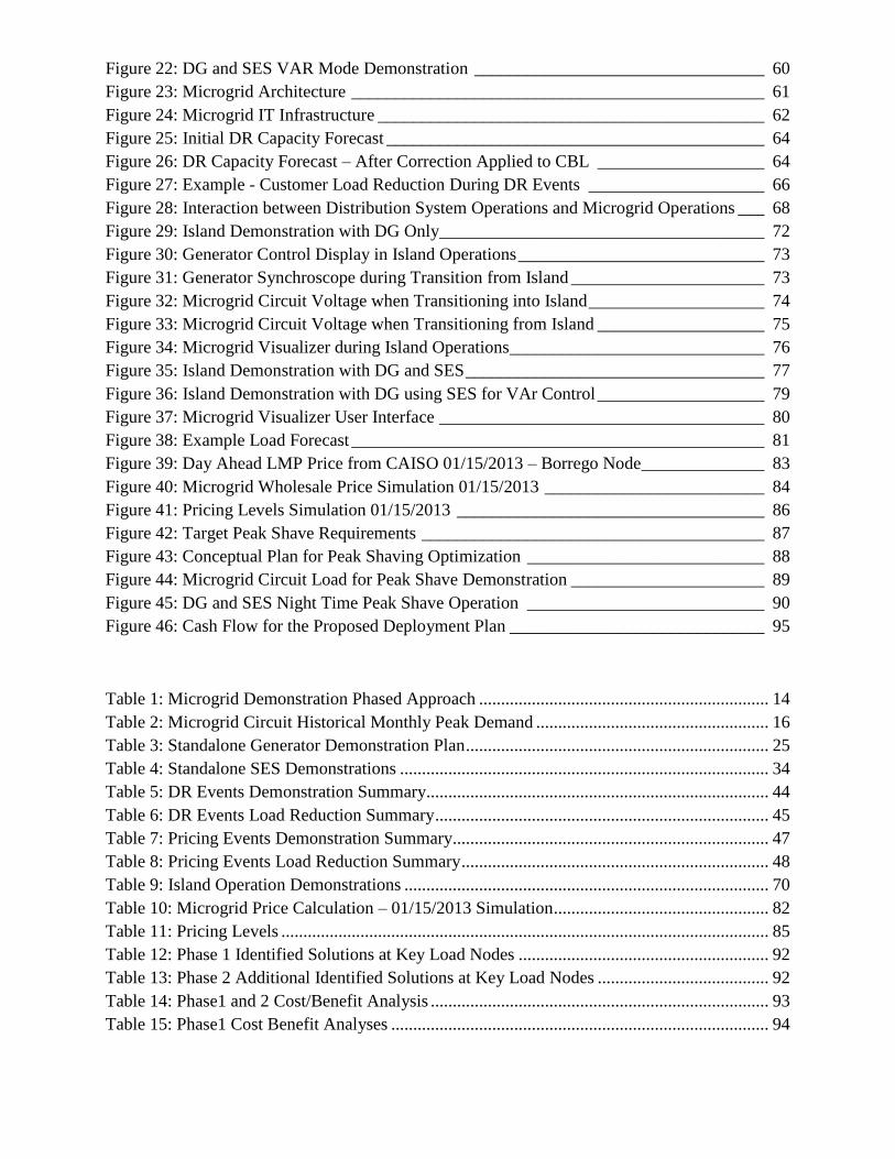
Figure 22: DG and SES VAR Mode Demonstration _________________________________ 60
Figure 23: Microgrid Architecture _______________________________________________ 61
Figure 24: Microgrid IT Infrastructure ____________________________________________ 62
Figure 25: Initial DR Capacity Forecast ___________________________________________ 64
Figure 26: DR Capacity Forecast – After Correction Applied to CBL ___________________ 64
Figure 27: Example - Customer Load Reduction During DR Events ____________________ 66
Figure 28: Interaction between Distribution System Operations and Microgrid Operations ___ 68
Figure 29: Island Demonstration with DG Only_____________________________________ 72
Figure 30: Generator Control Display in Island Operations ____________________________ 73
Figure 31: Generator Synchroscope during Transition from Island ______________________ 73
Figure 32: Microgrid Circuit Voltage when Transitioning into Island ____________________ 74
Figure 33: Microgrid Circuit Voltage when Transitioning from Island ___________________ 75
Figure 34: Microgrid Visualizer during Island Operations _____________________________ 76
Figure 35: Island Demonstration with DG and SES __________________________________ 77
Figure 36: Island Demonstration with DG using SES for VAr Control ___________________ 79
Figure 37: Microgrid Visualizer User Interface _____________________________________ 80
Figure 38: Example Load Forecast _______________________________________________ 81
Figure 39: Day Ahead LMP Price from CAISO 01/15/2013 – Borrego Node ______________ 83
Figure 40: Microgrid Wholesale Price Simulation 01/15/2013 _________________________ 84
Figure 41: Pricing Levels Simulation 01/15/2013 ___________________________________ 86
Figure 42: Target Peak Shave Requirements _______________________________________ 87
Figure 43: Conceptual Plan for Peak Shaving Optimization ___________________________ 88
Figure 44: Microgrid Circuit Load for Peak Shave Demonstration ______________________ 89
Figure 45: DG and SES Night Time Peak Shave Operation ___________________________ 90
Figure 46: Cash Flow for the Proposed Deployment Plan _____________________________ 95
Table 1: Microgrid Demonstration Phased Approach .................................................................. 14
Table 2: Microgrid Circuit Historical Monthly Peak Demand ..................................................... 16
Table 3: Standalone Generator Demonstration Plan ..................................................................... 25
Table 4: Standalone SES Demonstrations .................................................................................... 34
Table 5: DR Events Demonstration Summary.............................................................................. 44
Table 6: DR Events Load Reduction Summary ............................................................................ 45
Table 7: Pricing Events Demonstration Summary........................................................................ 47
Table 8: Pricing Events Load Reduction Summary ...................................................................... 48
Table 9: Island Operation Demonstrations ................................................................................... 70
Table 10: Microgrid Price Calculation – 01/15/2013 Simulation ................................................. 82
Table 11: Pricing Levels ............................................................................................................... 85
Table 12: Phase 1 Identified Solutions at Key Load Nodes ......................................................... 92
Table 13: Phase 2 Additional Identified Solutions at Key Load Nodes ....................................... 92
Table 14: Phase1 and 2 Cost/Benefit Analysis ............................................................................. 93
Table 15: Phase1 Cost Benefit Analyses ...................................................................................... 94

List of Acronyms and Abbreviations
AC Alternating Current
LMP Locational Marginal Pricing
AES Advanced Energy Storage
M&V Measurement and Verification
AMI Automated Metering Infrastructure
MDMS Meter Data Management System
C&I Commercial and Industrial
MMC Microgrid Master Controller
CAISO California Independent System Operator
MW Megawatt
CB Circuit Breaker
NOAA National Oceanic and Atmospheric Administration
CBA Cost Benefit Analysis
NOC Network Operations Center
CBL Customer Baseline Load
NPV Net Present Value
CEC California Energy Commission
O Other
CES Community Energy Storage
O&M Operations and Maintenance
CO Constant Output
OASIS Open Access Same-time Information System
DEM Distributed Energy Manager
OMS Outage Management System
DER Distributed Energy Resources
OpEx Operational Excellence
DG Distributed Generation
PCS Power Conversion System
DMS Distribution Management System
PCT Programmable Communicating Thermostat
DNP Distributed Network Protocol
PDLM Price Driven Load Management
DOE Department of Energy
PIER Public Interest Energy Research
DR Demand Response
PLC Programmable Logic Controller
EOC End of Circuit
PQ Power Quality
FAST Feeder Automation System Technology
PS Peak Shaving
FLISR Fault Location Isolation and Service Restoration
PV Photovoltaic
HAN Home Area Network
RDO Real Device Outage
HHV Higher Heating Value
RES Residential Energy Storage
HPV High Penetration Photovoltaic
RFP Request for Proposal
IHD In Home Display
RTP Real Time Pricing
ITC Investment Tax Credit
SCADA Supervisory Control and Data Acquisition
kBTU Kilo British Thermal Unit
SDG&E San Diego Gas and Electric
kVAr Kilo Volt Ampere Reactive
SES Substation Energy Storage
kW Kilowatt
SOC State of Charge
kWh Kilowatt-Hour
US United States
LCS Load Control Switch
VAr Volt Amp Reactive
LF Load Following
WP Weak Point
Acknowledgements
The Microgrid Demonstration Project was conducted with support of the following partners and
key vendors:
Partners
US Department of Energy
California Energy Commission
San Diego Gas and Electric
Vendors:
Horizon Energy Group
Saft with Parker Hannifin
Lockheed Martin
Hawthorne Power Systems

Final Technical Report
Page 6
1 Executive Summary
SDG&E has been developing and implementing the foundation for its Smart Grid platform for
three decades – beginning with its innovations in automation and control technologies in the
1980s and 1990s, through its most recent Smart Meter deployment and re-engineering of
operational processes enabled by new software applications in its OpEx 20/20 (Operational
Excellence with a 20/20 Vision) program. SDG&E’s Smart Grid deployment efforts have been
consistently acknowledged by industry observers. SDG&E’s commitment and progress has been
recognized by IDC Energy Insights and Intelligent Utility Magazine as the nation’s “Most
Intelligent Utility” for three consecutive years, winning this award each year since its inception.
SDG&E also received the “Top Ten Utility” award for excellence in Smart Grid development
from GreenTech Media.
This demonstration project brings circuit and customer realities to the picture. While a few
Microgrid trials have taken place in the US, they have typically been of a smaller scale and not
directly applicable to the real operating environment. This project differs from previous efforts
and has extended the knowledge base as follows:
The Microgrid supported actual customers in a real operating environment
The project is at significant scale (4MW)
The Microgrid design incorporates both reliability and economic oriented operations
Microgrid operations investigate the technical and economic interactions of multiple
resources
The project investigates the ability to use pricing signals to guide operations
The Project focused on the design, installation, and operation of a community scale “proof-of-
concept” Microgrid demonstration. The site of the Microgrid was an existing utility circuit that
had a peak load of 4.6 MW serving 615 customers in a remote area of the service territory. The
project focused on the installation, integration and operation of the following key technologies:
Distributed Energy Resources (Diesel Generators)
Advanced Energy Storage
Feeder Automation System Technologies
Price Driven Load Management
Integration with OMS/DMS and Microgrid Controls
The overall objectives for the Microgrid Demonstration Project were to:
1. Demonstrate the ability to achieve a 15% or greater reduction in feeder peak load
2. Demonstrate capability of reactive power management
3. Develop a strategy and demonstration of information integration focused on both security
and overall system architecture
4. Develop a strategy and demonstrate the integration of AMI into Microgrid operations

Final Technical Report
Page 7
5. Develop a strategy and demonstrate ‘self-healing’ networks through the integration of
Feeder Automation System Technologies (FAST) into Microgrid operations
6. Develop a strategy and demonstrate the integration of an Outage Management
System/Distribution Management System (OMS/DMS) into Microgrid operations
7. Demonstrate the capability to use automated distribution control to intentionally island
customers in response to system problems
8. Develop information/tools addressing the impact of multiple DER technologies
The project was unique in that the it was funded by the US Department of Energy (DOE), the
California Energy Commission (CEC), San Diego Gas and Electric (SDG&E), and the project
partners. There were two DOE funded activities that included the overall Microgrid Project and
then the inclusion of Community Energy Storage (CES) systems integrated into the Microgrid.
The CEC portion of the project addressed the customer-side of the meter resources related to the
Price Driven Load Management that consisted of the software cost, software installation, home
area network equipment cost, and installation in customer homes.
The project was conducted in three phases:
Phase 1: Baseline and Key Developments
Phase 2: Integration and Operational Testing
Phase 3: Data Collection and Analysis
The Phase 2 activities were carried out in an incremental fashion where a technology was
installed and operated to quantify its contribution to the Microgrid before the next technology
was added. Operations were conducted for each technology in a stand-alone basis and then in
combination with the other installed resources. Once all the resources were installed and the
stand-alone operations evaluated, demonstrations of Optimized operations were conducted. The
key elements of the Microgrid resources implemented for the project were:
Two 1,800 kW Diesel Generators
One 500 kW / 1,500 kWh lithium ion energy storage unit
A Fault Location, Isolation and Service Restoration system
An automated demand response system with pricing based event capabilities
A Microgrid Visualizer to support control and monitoring of the Microgrid resources
Diesel Generator Demonstrations
The key findings from this demonstration that lay a foundation for feeder optimization are:
The generators were able to operate in both constant output and load following modes
The generators were capable of operation using both local controls and remote control
through the Microgrid Visualizer
The generators were capable of operation individually and in conjunction with each other
The generators were capable of limiting the load at the Microgrid Circuit Breaker when
operated in the load following mode

Final Technical Report
Page 8
At certain times, the generators were capable of carrying the entire Microgrid Circuit load
(demonstrated by the zero flow at the breaker demonstrations)
The utility was able to develop and successfully execute a procedure between the
Microgrid Operator and Distribution System Operator to engage the operation of the
generators on the circuit on a routine basis
In planned operations, the generators could be started, warmed up, synchronized to the
grid, and operated at the desired set point in approximately 10 minutes
The generators operated very close to the manufacturer’s performance curve
Fault Location, Isolation and Service Restoration (FLISR) System Demonstrations
The FLISR demonstrations were conducted as simulations using the new outage management
system and distribution management system (OMS/DMS). The simulations validated the control
algorithms and the ability of the system to present the correct switching plans to the distribution
operators. The simulation validated that the use of FLISR can result in the distribution operators
being able to address faults and restore the maximum number of customer within a period of five
minutes. This means that many outages can be managed so that a minimum number of customers
experience a momentary outage instead of a longer sustained outage.
Energy Storage System Demonstrations
The key findings from this demonstration that lay a foundation for feeder optimization are:
The energy storage system was able to operate in both constant output and load following
modes
The energy storage system was capable of operation using both local controls and remote
control through the Microgrid Visualizer
The energy storage system was capable of limiting the load at the Microgrid Circuit
Breaker when operated in the load following mode
The utility was able to develop and successfully execute a procedure between the
Microgrid Operator and Distribution System Operator to engage the operation of the
energy storage system on the circuit on a routine basis
The energy storage system efficiency and capacity were near the manufacturer’s
performance specifications. The demonstrated performance was a round trip efficiency
of 87.1% and a total storage capacity was 1,718 kWh.
VAr demonstrations showed that the energy storage system is able to control the reactive
power at the circuit breaker in a manner similar to a variable capacitor
The energy storage system is capable of four quadrant operation

Final Technical Report
Page 9
Price-Driven Load Management (PDLM) Demonstrations
The Price-Driven Load Management system was used for managing customer load on the
Microgrid. The PDLM system was interfaced with SDG&E’s newly deployed advanced
metering infrastructure system and included Home Area Network (HAN) systems, and the
PDLM controller. Customer-side technologies that integrate into the PDLM system are:
Programmable Communicating Thermostats
Load Control Switches
Plug Load Controllers
In-Home Displays
Customer Web Portal
The PDLM controller is the system of record to forecast Demand Response (DR) capacity and
schedule DR events to meet the load reduction objectives within the Microgrid.
A major objective of the demonstration project was to discover how the PDLM resources could
be managed in the Microgrid environment and if PDLM could be managed like the other DER
resources. Ideally, PDLM could be managed in the Microgrid the way that generators or storage
systems are managed.
The PDLM system is limited and constrained by the capacity to deliver load reduction depends
on weather, time of day, and customer behavior. Agreements with customers limited the
frequency and duration of PDLM events during the demonstration. Customers also had the
option to opt-out of events. One of the methods employed for the demonstration to help manage
Microgrid resources was to have the PDLM system forecast the demand reduction capacity on an
hourly day-ahead basis. The forecasts that were developed were not as accurate as needed and
the approach for improving the forecast required many iterations of events which were limited.
Taken together, PDLM is very different from the other DER resources in the Microgrid. While it
can be dispatched as part of the overall Microgrid Optimized plan, benefiting from PDLM
requires a wider variety of operational considerations and is far less reliable and predictable than
other resources in its current design.
Microgrid Island Demonstrations
One of the highlights of the Demonstration project was the ability to effectively island the entire
Microgrid supporting more than 600 customers. The islanding demonstrations transitioned into
and out of the island mode without affecting the quality of service to the customers (seamless
transitions without an outage or flicker). The island demonstrations evaluated the island
operations with the DG units only, the DG units operating with the SES in both charge and
discharge modes, and the DG units operating with the SES unit providing a majority of the
reactive power requirements. All demonstrations were successful and fulfilled the stated
operational objectives.
Additionally, the Microgrid was operated in island operation twice during the demonstration
period to provide service to customers who would have otherwise had an extend loss of service.

Final Technical Report
Page 10
One event occurred for a planned upgrade to the substation to accommodate the connection of a
26 MW PV system. The other event was during an unplanned outage that was caused by bad
weather. In both instances the Microgrid substation configuration was changed to successfully
island over 1000 customers.
Cost Benefit and Future Deployments
The lessons learned and the quantified benefits from the Microgrid demonstration were used to
identify other potential cost effective Microgrid applications in the SDG&E service territory.
Applications were identified where there is a high potential to improve existing distribution
operations (i.e. highest benefit potential) and classified as follows:
Large commercial and industrial customers
Communities with challenges due to a high penetration of solar PV
Weak points in the distribution network
End of circuit
Other
The key findings from the cost benefit analysis are that potential deployment of cost-effective
Microgrids and DER are not as broad and deep as expected. A total of 28 cost-effective
applications were identified for further consideration in the service territory:
10 MW Microgrid: quantity = 2
1 MW Microgrid: quantity = 10
300 kW DER solutions: quantity = 18
Please Note: The Borrego Springs Microgrid Demonstration Project was done in conjunction
with work funded by the California Energy Commission (CEC). For additional information and
findings, please refer to the PIER Final Project Report entitled Borrego Springs Microgrid
Demonstration Project - CEC-500-08-025.

Final Technical Report
Page 11
2 Introduction
The foundation of existing electric utility systems is based on delivering power from central
station generation units to a diverse group of end users. Market, technological, and regulatory
forces have created a nexus of opportunity to leverage distributed resources in the delivery of
highly reliable and cost effective electricity through a Smart Grid alternative service delivery
model (Microgrid). At the same time, customers are also investigating and investing in energy
assets and distribution systems for their facilities ranging from backup power systems to on-site
generation to renewable energy resources. While some progress has been made on the
development of interconnected loads and distributed energy resources there has been scant
attention to the development of an integrated energy system that can operate in parallel with the
grid or in an intentional island model. Hence, there a critical need to understand how Microgrids
consisting of interconnected loads and distributed energy resources can be operationally
optimized and developed in a cost effective manner. Concurrently, there is an increasing need to
assess the role, impact, and contributions of sustainable communities in integrated Microgrid
designs and their potential to contribute to demand response objectives and programs.
San Diego Gas and Electric (SDG&E) embarked on The Borrego Springs Microgrid
Demonstration Project to design and implement an innovative Microgrid that integrates the
electrical distribution network, distributed energy resources and resources on the customer-side
of the meter. The design focused on the ability to optimize assets, manage costs, and increase
reliability. Enabling technologies to be integrated in the Microgrid included automated demand
response, distributed generation, advanced energy storage, and outage management technologies.
This demonstration project also lays the framework for assessing cost versus benefits and the
impact and viability of Microgrids on energy costs and price volatility.
The project brings circuit and customer realities to the picture. While a few Microgrid trials have
taken place in the US, they have been small scale and not directly applicable to the real operating
environment. This project differs from previous efforts and has extended the knowledge base as
follows:
The Microgrid supported actual customers in a real utility operating environment
The project is at significant scale (4 MW)
The Microgrid design incorporates both reliability and economic oriented operations
Microgrid operations investigate the technical and economic interactions of multiple
resources
The project investigates the ability to use pricing signals to guide operations
The project was designed to operate at a real world scale with more than 600 actual customers,
and was affected by operations such as outage, transient, and event conditions. The project
provided knowledge about the design, operational, and economic considerations of an integrated
Microgrid system. The successful and optimized integration of distributed energy technologies
not only rests with their functionality and ability to address outages and event conditions, but
also the economics of Microgrids.

Final Technical Report
Page 12
The design and implementation of the Microgrid also meant the involvement of a large cross
section of departments and personnel at SDG&E. This included personnel from Asset
Management, Transmission and Distribution System Operations, Customer Programs,
Regulatory, Research and Development, Emerging Technologies, and Information Technology
and Security. This demonstration provided in depth experience to SDG&E personnel and
stakeholders alike, on the scale of resources that are required to implement Microgrids that affect
real customers and electric operations.
This project consisted of several team members and was funded by a United States Department
of Energy (DOE) Renewable and Distributed Systems Integration grant, a California Energy
Commission’s PIER grant and cost share by SDG&E and other project team members provided
the remaining funds for the demonstration. The CEC PIER portion of the project focused on the
integration of resources on the customer-side of the meter and evaluated their contribution to
Microgrid operations.
Section 3 of this report presents the overall objectives that were achieved for the Microgrid
Demonstration. Section 4 presents the phased approach that was developed to integrate the
various technologies and strategies. Section 5 provides a summary of the key findings based on
the project objectives. Section 6 presents the Microgrid deployment scenario within the SDG&E
service territory. Lessons Learned and Key Findings are presented in Section 7.

Final Technical Report
Page 13
3 Objectives
The Project consisted of a full scale “proof-of-concept” demonstration of a Microgrid on an
existing utility circuit that had a peak load of 4.6 MW serving 615 customers in a remote area of
the service territory. The project focused on the installation, integration and operation of the
following key technologies:
Distributed Energy Resources (Diesel Generators)
Advanced Energy Storage
Feeder Automation System Technologies
Price Driven Load Management
Integration with OMS/DMS
Microgrid Controller
The overall objectives for the Microgrid Demonstration Project were to:
1. Demonstrate the ability to achieve a 15% or greater reduction in feeder peak load through
the integration of multiple, integrated DER – distributed generation (DG), electric energy
storage, and price driven load management on a San Diego Gas and Electric Company
feeder
2. Demonstrate capability of Volt-Amps-Reactive (VAr) electric power management -
coordinating the DER with existing VAr management/compensation tools
3. Develop a strategy and demonstration of information integration focused on both security
and overall system architecture
4. Develop a strategy and demonstrate the integration of AMI into Microgrid operations
5. Develop a strategy and demonstrate ‘self-healing’ networks through the integration of
Feeder Automation System Technologies (FAST) into Microgrid operations
6. Develop a strategy and demonstrate the integration of an Outage Management
System/Distribution Management System (OMS/DMS) into Microgrid operations
7. Demonstrate the capability to use automated distribution control to intentionally island
customers in response to system problems
8. Develop information/tools addressing the impact of multiple DER technologies
including:
o Control algorithms for autonomous DER operations/automation that address multiple
DER interactions and stability issues
o Penetration limits of DER on the substation/feeder
o Coordination and interoperability of multiple DER technologies with multiple
applications/customers.

Final Technical Report
Page 14
4 Approach
The project plan was organized into three phases:
Phase 1: Baseline and Key Developments
Phase 2: Integration and Operational Testing
Phase 3: Data Collection and Analysis
Table 1 presents the phased approach that was developed to integrate the various technologies
and strategies and provides an outline of the tasks associated with each Phase of the project.
Table 1: Microgrid Demonstration Phased Approach
Phase Task
Phase 1 -Establishment of
Baseline and
Key Developments
Task 1B --Site Selection
Task 2.1 -- Pilot Network Analysis and Baselining
Task 2.2 -- Key Developments
Phase 2 – Integration of
Technologies and
Operational Testing
Task 3.1 -- Integration of Existing Distributed Energy Resources and
VAr Compensation
Task 3.2 -- Stage 1 Distributed Systems Integration (DSI) Testing
Task 3.3 -- Integration of Feeder Automation System Technology
Task 3.4 -- Stage 2 Distributed Systems Integration Testing
Task 3.5 -- Integration of Advanced Energy Storage
Task 3.6 -- Stage 3 Distributed Systems Integration Testing
Task 3.7 -- Integration of Outage Management System/Distribution
Management System (OMS/DMS) for Microgrid Operations
Task 3.8 -- Stage 4 Distributed Systems Integration Testing
Task 3.9 -- Integration of Price-Driven Load Management
Task 3.10 -- Stage 5 Distributed Systems Integration Testing
Task 3.11 -- Feeder Optimization Scenario Testing
Phase 3 – Data Collection and
Analysis
Task 5.1 -- Cost / Benefit Analysis for Large-Scale Deployment
Task 5.2 -- Implementation Plan for Large-Scale Deployment
4.1 Phase 1 - Establishment of Baseline and Key Developments
Phase 1 of the project involved establishing a baseline for a selected circuit within the service
territory. A substation was selected after performing a detailed site selection process. A network
analysis was performed on the selected circuit to collect historical data to establish the baseline
operational performance characteristics of the associated substation and selected circuit in terms
of key metrics such as load profiles and reliability metrics. This data served as the basis for
developing specific strategies of equipment sizing, interface requirements, operating scenarios,
and created a foundation to measure the anticipated impacts of the various Microgrid Resources.
Key developments for the Project included a comprehensive set of Use Cases that were used to

Final Technical Report
Page 15
identify departments within the utility that would need to be involved in the Project, the
anticipated sequence of operations, technology functional requirements, communication
requirements, and cyber security considerations. This process was key to the project as this
foundation was used as a source for the development of Request For Proposals for the Microgrid
Resources including the, generator control upgrade, advanced energy storage, the Price Driven
Load Management System, and the Microgrid Controller.
Task 1B - Site Selection
The process of site selection was based on criteria that addresses substation, circuit and customer
attributes. The site selection team evaluated 18 substations using an evaluation matrix that
addressed the following factors with an emphasis on meeting project goals and improving
reliability:
Permitting requirements
Level of AMI penetration
Level of customer-owned renewable resources
Environmental requirements
Communications environment
Existing customer-owned non-renewable generation resources
Anticipated community acceptance of the Microgrid project
Potential customer participation in Energy Efficiency and DR programs
Potential distribution system impacts on peak load and reliability
Transmission system impacts on peak load, reliability, and congestion pricing
A circuit served by the Borrego Substation was selected as the Microgrid Circuit due to the
following characteristics:
Relatively high penetration of customer-owned PV
Potential for improvement in reliability
Availability of land adjacent to the substation
Reasonable peak load in the circuit (4.6 MW)
Remote location
Few customers near the substation
Mostly residential customers on circuit
Some challenges that the Borrego substation presented include:
No AMI infrastructure (at the time of selection)
Substation located in a 100 year flood plain
Need to work with the community to gain acceptance
Remote area
Potential communication issues
No natural gas infrastructure

Final Technical Report
Page 16
Population fluctuates with the seasons (higher in the winter and lower in the summer)
Desert climate (summer high temperatures greater than 110 oF)
The Borrego substation is located at the end of a single radial 69 kV transmission line. At the
substation, the voltage is stepped down to 12 kV and serves three radial distribution circuits.
Task 2.1 - Pilot Network Analysis and Baselining
A performance baseline was established by identifying and collecting key Microgrid Circuit
metrics. This baseline provided the basis for comparison with the data collected during the
demonstrations. The existing system infrastructure on the Microgrid Circuit included the
following devices:
SCADA enabled switches
Voltage Regulators
Capacitors
Microwave Communication System
Historical data on the Microgrid Circuit was analyzed to develop daily load profiles for each year
during the period between 2007 and 2009. Table 2 and Figure 1 present a summary of the
monthly peak demand for the Microgrid Circuit. The data shows a trend with higher peak
demand in the summer with an average peak of 4.3 MW. The highest peak of 4.6 MW occurred
in August 2009. The lack of significant yearly variability is due to the significant population
swings.
Table 2: Microgrid Circuit Historical Monthly Peak Demand
Month 2007 2008 2009 Average
Jan 4.12 3.38 4.21 3.90
Feb 3.58 3.29 3.50 3.46
Mar 3.75 3.48 3.70 3.64
Apr 3.7 3.62 3.54 3.62
May 4.03 3.76 3.89 3.89
Jun 4.11 3.98 4.08 4.06
Jul 4.32 4.22 4.48 4.34
Aug 4.12 4.1 4.63 4.28
Sep 3.84 3.86 4.48 4.06
Oct 3.05 3.69 3.94 3.56
Nov 2.63 3.59 3.23 3.15
Dec 3.45 3.45 2.66 3.19
Max 4.32 4.22 4.63 4.34
Final Technical Report
Page 17
Figure 1: Microgrid Circuit Historical Monthly Peak Demand
Hourly data was analyzed to gain a better understanding of the load characteristics on the
Microgrid Circuit. Figure 2 presents the hour summer day profiles for July 2009 with each line
representing a day of the month. This data shows that the circuit has a unique load profile in that
the day-time load is low and the circuit peak load occurs at night. The high night time load is
because of the use of water pumps by the local water district and irrigation pumps by agriculture
customers on the circuit. These customers are on a time-of-use tariff where the demand charges
and energy rates are lower during the night.
Figure 2: Summary Hourly Load Profiles for the Month of July 2009
There are a total of 26 customer-owned PV systems on Microgrid Circuit with a total installed
inverter capacity of 597 kW. The system sizes range from 225 kW down to 2 kW. There are
2.0
2.5
3.0
3.5
4.0
4.5
5.0
Jan Feb Mar Apr May Jun Jul Aug Sep Oct Nov Dec
De
ma
nd
(M
W)
Month
Circuit A Historical Peak Demand
2007 2008 2009 Average
0.0
0.5
1.0
1.5
2.0
2.5
3.0
3.5
4.0
4.5
5.0
0:1
5
1:1
5
2:1
5
3:1
5
4:1
5
5:1
5
6:1
5
7:1
5
8:1
5
9:1
5
10:1
5
11:1
5
12:1
5
13:1
5
14:1
5
15:1
5
16:1
5
17:1
5
18:1
5
19:1
5
20:1
5
21:1
5
22:1
5
23:1
5
Dem
an
d (
MW
)
Time
Circuit A- July 2009

Final Technical Report
Page 18
two 225 kW customer-owned systems on the circuit. Detailed analysis was performed to estimate
the annual electric production for the PV systems on the Microgrid Circuit.
Figure 3 presents a graph of the daily AC output of the aggregated PV systems on the Microgrid
Circuit for a typical summer month of July. Daily PV load profiles are presented in different
colors for each day of the month.
Figure 3: Aggregated Daily AC Output for the Microgrid Circuit PV Systems - July (Typical Year)
Operation of the Microgrid Resources needs to be able to address the intermittency of this PV
generation.
Task 2.2 – Key Developments
Use cases were developed with a group of stakeholders that included subject matter experts from
numerous SDG&E departments, vendors, and project partners. These use cases captured various
scenarios for operation and control of the distributed energy resources within the Microgrid. In
all, ten Use Cases were identified and many had more than one scenario that was analyzed and
documented. A summary of the Use Cases and scenarios are as follows:
Use Case 1: Utility Manages Utility-Owned Distributed Generation
Scenario 1: Utility uses communications infrastructure to communicate with utility-
owned distributed generation to start/stop generator in constant output mode.
Use Case 2: Real-time VAR Support
Scenario 1: Capacitor reads Circuit VAr data real time and automatically turns on or off
based upon prearranged setting. Change in status reported to DMS through SCADA.
Scenario 2: Capacitor reads line voltage and relays it to DMS through SCADA.
Scenario 3: Distribution operator places capacitor in Manual mode and manually turns
capacitor on or off and Microgrid Master Controller (MMC) re-optimizes.
Use Case 3: FAST
Scenario 1: Microgrid in island operation, a fault occurs inside Microgrid.
0.00
0.05
0.10
0.15
0.20
0.25
0.30
0.35
0.40
0.45
0:1
5
1:1
5
2:1
5
3:1
5
4:1
5
5:1
5
6:1
5
7:1
5
8:1
5
9:1
5
10:1
5
11:1
5
12:1
5
13:1
5
14:1
5
15:1
5
16:1
5
17:1
5
18:1
5
19:1
5
20:1
5
21:1
5
22:1
5
23:1
5
Dem
an
d (
MW
)
Time
Microgrid Circuit - July (Typical Year)

Final Technical Report
Page 19
Scenario 2: Microgrid in island operation on DG only, a fault occurs inside Microgrid.
Scenario 3: Microgrid in island operation on AES with DG available, a fault occurs
inside Microgrid.
Scenario 4: Capacitor automatically comes online or offline as a result of FAST
operation.
Use Case 4: Independent Energy Storage Operations
Scenario 1: Energy storage executes charge/discharge sequence independent of DMS and
MMC control as part of ongoing Peak Shaving Operations (similar to Capacitor Bank
operations)
Scenario 2: Energy storage executes charge/discharge sequence in response to over
voltage or under voltage on circuit (load-following mode)
Use Case 5: Directed Energy Storage Operations
Scenario 1: Energy storage executes basic charge/discharge sequence due to command
from DMS/MMC
Scenario 2: Energy Storage executes change in VAr flow during charge/discharge
operations due to request from DMS/MMC. SCADA capacitor detects change in VAr
status and reacts accordingly
Scenario 3: Utility uses energy storage for energy arbitrage (financial)
Use Case 6: MMC monitors grid system status and exerts control to maintain system
stability and prevent overloads
Scenario 1: MMC detects line outage, arms appropriate response, and executes
Scenario 2: Microgrid executes a planned transition to island operation
Scenario 3: Microgrid reconnects to the main grid
Scenario 4: MMC controls individual Microgrid resources
Use Case 7: MMC monitors grid system status and passes information along to DMS
Scenario 1: MMC incorporates all system information into a status evaluation
Use Case 8: MMC curtails customer load for grid management due to forecast
Scenario 1: Forecast load expected to be subject to curtailment and pass to DMS
Scenario 2: Execute curtailment in response to pre-scheduled pricing event on system
Scenario 3: Customer opts out of curtailment for pre-scheduled event
Scenario 4: Load at the customer site is already below threshold
Scenario 5: Forecast DR event incorporating 3rd party aggregators with localized control
and measurement capabilities
Use Case 9: MMC curtails customer load for grid management due to unforeseen events
Scenario 1: Execute emergency curtailment in response to load on system

Final Technical Report
Page 20
Scenario 2: Customer opts out of curtailment for Grid Management (same as scenario 1)
Scenario 3: Customer already operating at DR commitment level (same as scenario 1)
Use Case 10: Planners Perform Analyses Using Multiple Data Sources
Scenario 1: Planners perform studies with data from a designated subset of meters
Microgrid Design - The Microgrid conceptual design was created from the use case
requirements that include the objective of managing peak load on the Microgrid Circuit to
improve reliability and circuit operation. Design discussions were conducted to develop an
operational methodology for design and integration of the Microgrid Resources in two major
modes:
Normal mode (grid-connected) - In this mode of operation, the Microgrid Resources support the
electric service provided by the grid. These resources are managed to achieve the following
operational objectives:
Peak Demand Reduction
Reliability
Economics
Environmental Factors
Island Operation - In this mode of operation, the Microgrid is isolated from the grid and the
Microgrid Resources are managed to ensure a balance between generation and load. Two
approaches to the Microgrid island mode of operation were evaluated:
Planned Island: The planned Island would occur during a planned outage of the circuit or
for transmission line maintenance or upgrades.
Unplanned Island: The unplanned Island would occur after a fault that results in an
extended outage. To operate in the unplanned island, a sequence of operation was
developed to sectionalize the circuit for load management, cold start of the generator
units, forecast of system load, and restoration of the customers within the Microgrid.
In both approaches to Island Operation, the Microgrid generation resources need to have the
capability to synchronize back to the grid in a managed transition once the service to the
Microgrid Circuit is restored.
Control Methodology - Both a centralized control methodology and a distributed control
methodology were considered. A distributed level of control has been successfully applied to
managing operations of the main grid. This same method was used as a starting point for
evaluating the best control methodology for the Microgrid.
Centralized Control - All control actions for the Microgrid would be centralized under the
Microgrid Controller as a component of the Distribution Management System (DMS). A
centralized control methodology simplifies Microgrid operations and its integration with other
distribution systems and processes. However, this was deemed impractical for a number of
reasons:

Final Technical Report
Page 21
Centralized control is not feasible due to the rapid response needed to address expected
transients in real time
Centralized control is the control method of choice only for non-critical applications that
can be applied over many seconds to minutes
Centralized control is vulnerable to single points of failure in communication or even loss
of Microgrid Controller functionality
Communications require very high speed, low latency, and extremely high reliability to
support the real time response to transients required by Microgrid resources
Distributed Control- It is a combination of centralized control and decentralized control. In this
model, the Microgrid Controller is responsible for dispatching Microgrid Resources and high
level data collection and analysis. This model is similar to the approach used for the utility
distribution operations with some exceptions:
In parallel operation, the main grid maintains system frequency within limits. The main
grid responds to Microgrid transients without action from the Microgrid control systems.
Power quality (PQ) and voltage are exceptions. Local controls at the Microgrid resources
adjust voltage regulators and inverters to achieve PQ and voltage set points. Centralized
control from the Microgrid Controller adjusts set points of the Microgrid resources over a
longer timeframe to optimize the performance.
In island mode, the inertial response provided by the main grid is not available. The
Microgrid is more sensitive to upsets and transients. Decentralized local controls at the
Microgrid resources are useful in responding to changes in frequency and voltage. This
action is analogous to the action provided by governor and voltage regulators at power
plants connected to the main grid. The primary objective is reliability, stability and PQ
within limits. Secondary objectives are efficiency, economics, and environmental
metrics.
The Microgrid Controller provides centralized control in parallel and island modes of Microgrid
operation. It operates over a longer time horizon and dispatches Microgrid Resources by
adjusting operating set points to achieve operating and optimization objectives. The Microgrid
Resources have their own local controls for distributed control including system operation and
protection. These specific systems provide for individual control to turn the equipment on and
off, set the mode of operation, accept changes to operating set points, and trigger operational
events.
4.2 Phase 2 - Integration of Technologies and Operational Testing
Task 3.1 – Integration of Existing Distributed Energy Resources and VAr Compensation
Two Caterpillar XQ-2000 Power Modules with CAT 3516TA Diesel Engine Generators were
used as the Distributed Generation (DG) component of the Microgrid as shown in Figure 4. Each
generator has a nominal generation capacity of 1,800 kW.

Final Technical Report
Page 22
Figure 4: Microgrid Distributed Generators
These units can be controlled locally at the substation or using a secure remote interface. The DG
units can operate in the following modes of operation:
Base Load (Constant Output) – This operational mode of the generator(s) is applicable
when the generator(s) are running in parallel with the main grid. The generator(s) in base-
load operates at set points to produce real power (kW) at a given power factor setting.
Import Control (Peak Shaving) – This operational mode of the generator(s) is applicable
when the generator(s) are running in parallel with the main grid. In this mode, the
generators maintain power flow (kW) through the Microgrid Circuit breaker at or below
the specified Import Control set point.
Island Operating Mode – In this operational mode, the generator(s) are loaded to meet the
demand (kW) on the Microgrid Circuit. The generator controller manages the frequency
and reactive power of the circuit.
DG Operational Constraints - The individual DG unit operating hours are restricted to 8 hours
per day and 200 hours per year by permits from the San Diego Air Pollution Control District
(SDAPCD).
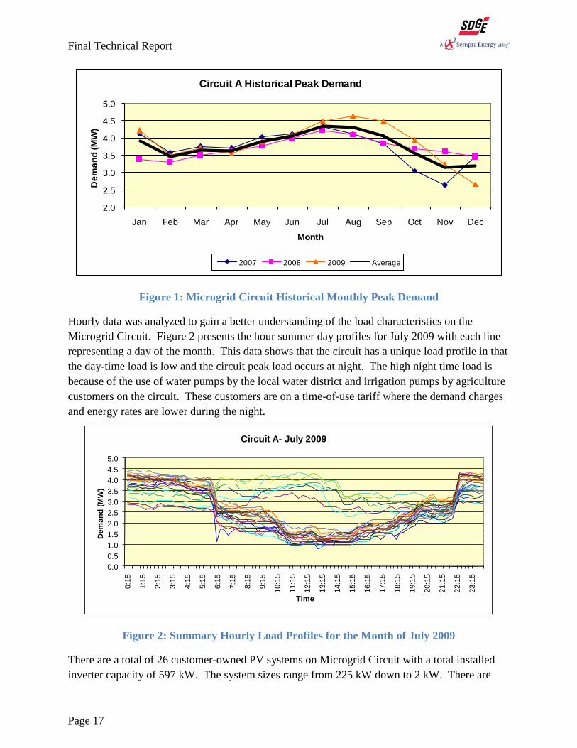
DG Heat Rate & Economic Cost Calculation - Heat Rate (kBTU/kWh) is the primary metric
for assessing the economics of generator operation on the basis of operational efficiency.
Performance data (heat rate and operational cost) from the generator manufacturer is presented in
Figure 5. It is based on a cost of $4.00/gallon for Ultra-Low-Sulfur Diesel and a diesel Higher
Heating Value (HHV) of 128,000 BTU/gallon.
Final Technical Report
Page 23
Figure 5: Baseline DG Heat Rate and Operational Cost
SCADA Integration and Protection System – The utility SCADA system was utilized to
provide coordinated operation of existing switches and breakers within and at the boundary of
the Microgrid Circuit. To maintain continuity with existing operations, the generator breaker
protection was integrated into the existing SCADA system via fiber-optic communications
between the generator breaker protection relays and the protection relay on the Microgrid Circuit
main breaker. The following SCADA commands were used to manage the switching actions to
transition the Microgrid between its various operating states.
Parallel Command - Enables a synchronized-check across the generator breaker, allowing
it to close when the generator output has matched frequency, voltage, and phase angle
with the Microgrid Circuit and connected substation.
Normal Command (Break Parallel) - This command forces the DG units to disconnect
(“break-parallel”) from the substation leaving the Microgrid Circuit supplied by only the
transmission network.
Island Command - Enables the generators to pick up the entire load of the Microgrid
Circuit. The generators operate to drive power flow to zero across the substation breaker.
When this is accomplished, the Microgrid Circuit main breaker is opened and the
Microgrid is separated from the substation and operating as an Island.
Black-Start Command - This command (in the event of complete loss of power to the
substation) enables a substation dead-bus check by the protection relay on the Microgrid
main breaker and opens the Microgrid main breaker. Further it facilitates the closing of
the generators into the dead bus, energizing the Microgrid Circuit in an Island operating
state.
$0.200
$0.250
$0.300
$0.350
$0.400
$0.450
$0.500
8.0
9.0
10.0
11.0
12.0
13.0
14.0
15.0
16.0
10 20 25 30 40 50 60 70 75 80 90 100
% of Rated Capacity
Op
era
tio
nal
Co
st: $
/kW
h
Hea
t R
ate
: kB
TU/k
Wh
CAT 2516B Heat Rate & Operational Costs
Heat Rate Operational Cost

Final Technical Report
Page 24
The DG controller’s operational mode selection, set points, and operational status are accessible
from a remote Microgrid Visualizer via secure communications. On the network communication
path, a dedicated Microgrid gateway was provided to the interface point for the generator
controllers. Network communications between the generator controllers and the gateway use
Modbus-IP protocol. Network communications between the Microgrid gateway and back-office
systems occurs via Distributed Network Protocol (DNP3).
Task 3.2 – Stage 1 Distributed Systems Integration (DSI) Testing
This task demonstrated the testing of the DG units on the Microgrid Circuit. The objective of
these demonstrations was to quantify the contributions of the DER and VAr compensation
components to the Microgrid. A component of the task was to compare the results from DG
operation to the baseline to determine relative improvements consistent with the objectives of the
Project. In addition, data collected from the demonstrations was used to validate the operational
efficiency of the units under varying load conditions and to compare actual efficiency to the
manufacturer’s published performance curves.
Four types of standalone generator demonstrations were conducted:
Constant Output - The constant output mode operation represents the most basic
operation of the generators and was used to get the operators acquainted with the steps
required to operate the equipment as well as learn how the generators respond to the
given commands. These demonstrations established the interface and coordination with
the Distribution Operators who provided the permissions and required switching
operations for the generators to synchronize with the Microgrid Circuit.
Peak Shave - The Peak Shave Mode represents one of the key modes of operation for the
generators in the Microgrid as it is the mode that will be required to meet the 15% peak
load reduction goal for the project. In the Peak Shave Mode, the generators monitor the
load at the Microgrid Circuit Breaker and supply the electricity required by the Microgrid
Circuit load that is in excess of the Microgrid Circuit Breaker Load Set point. The
primary objective of the Peak Shave Mode tests was to demonstrate the ability of the
generator’s controls to conduct the peak shaving operations and to observe the
characteristics of the control algorithms for this mode of operation.
Zero at the Breaker - The Zero Flow at the Breaker Demonstrations is a special case of
the Peak Shaving Mode Demonstrations. In this case, the generators are operated in Peak
Shave mode with a set point of zero kW. This mode is required when the Microgrid is
transitioning from grid connected to Island Mode. To seamlessly transition to an island,
the load at the breaker needs to be near to zero as the generators become the voltage and
frequency source for the circuit. The Zero Flow at the Breaker Demonstrations also
validate the ability for the two generators to operate in parallel while load following.
VAr Control - The primary objective of the VAr Mode demonstration was to demonstrate
the ability to have the generator provide VAr support to the circuit by adjusting the power
factor settings.

Final Technical Report
Page 25
Table 3 summarizes the standalone generator demonstrations that were conducted for this task.
The Table presents the mode, which combination of generators are involved, the date and time of
the operations, and the control interface used to conduct the operations.
Table 3: Standalone Generator Demonstration Plan
Task 3.3 – Integration of Feeder Automation System Technology
Integration of Feeder Automation System Technology (FAST) for the Microgrid project was
accomplished by the implementation of Fault Location, Isolation and Service Restoration
(FLISR) functionality as part of the installed Outage Management System and Distribution
Management System. The implementation and demonstration of the OMS/DMS FLISR system
included leveraging the existing OMS/DMS integration with the distribution network SCADA
system. The Microgrid Circuit was one of the initial circuits used to test and validate the
operation of the system.
There is a significant investment in infrastructure, tools, and training that support a Distribution
System Operator’s rapid response to unplanned events. The recent implementation of a new
Outage Management and Distribution Management System by the Utility are the foundation for
improved systems environment.
Among the DMS functions are the capabilities of using SCADA telemetry and status values to
recognize a fault location (“FL”) in the distribution network, apply power flow capabilities to
determine suggested switching alternatives and recommend a plan to isolate (“I”) the fault and
execute the steps necessary for service restoration (“SR”); FLISR.
Mode of
Operation
Demonstration
DescriptionControl Settings
Demonstration
Date
Start
Time
End
Time
Gen1 Gen2 Local Remote
X DG Constant Mode Demo A 1000/1250/1500 kW 06/12/12 9:05 10:20 X
X DG Constant Mode Demo A 1000/1250/1500 kW 06/12/12 10:15 11:30 X
X DG Constant Mode Demo B 750/1000/1250/1500 kW 02/25/13 9:05 10:00 X
X DG Constant Mode Demo B 750/1000/1250/1500 kW 03/04/13 10:20 11:15 X
X DG Constant Mode Demo C 1800 kW 03/12/13 10:25 11:55 X
X DG Constant Mode Demo C 1800 kW 03/12/13 9:50 10:45 X
X DG Constant Mode Demo C 1800 kW 03/14/12 9:30 13:00 X
X DG Constant Mode Demo C 1800 kW 03/15/12 8:15 12:00 X
X DG Constant Mode Demo C 1800 kW 03/14/12 13:10 17:50 X
X DG Constant Mode Demo C 1800 kW 03/28/12 9:20 10:15 X
X X DG Constant Mode Demo D 500/750/500 kW 01/08/13 11:20 12:40 X
X DG Constant Mode Demo D 1000 kW 01/08/13 9:30 10:15 X
X DG LF Peak Shave Iteration Demo A 300 kW 06/14/12 9:00 10:40 X
X DG LF Peak Shave Iteration Demo A 300 kW 06/14/12 10:37 12:17 X
X DG LF Peak Shave Iteration Demo B 500 kW 11/15/12 9:40 11:30 X
X DG LF Peak Shave Iteration Demo B 650 kW 11/15/12 13:20 14:20 X
X DG LF Peak Shave Iteration Demo B 500 kW 11/15/12 14:20 15:20 X
X DG LF Peak Shave Iteration Demo C 1000 kW 03/11/13 10:05 11:30 X
X DG LF Peak Shave Iteration Demo C Peak Shave of 15% 02/19/13 21:55 0:45 X
X XDG LF Virtual Island with Zero Flow at
Breaker Demo A0 kW (Import) 06/18/12 9:26 10:51 X
X XDG LF Virtual Island with Zero Flow at
Breaker Demo A0 kW (Import) 11/16/12 10:20 12:20 X
X DG VAr Control Demo Setpoint-A 50/100 kVAr 01/08/13 11:20 12:45 XVAr Control
Microgrid
Resource
Constant Output
Peak Shave
Zero at Breaker
Control Interface

Final Technical Report
Page 26
A metric used to measure outages is Momentary Average Interruption Frequency Index
(MAIFI); momentary outages are defined as customers affected less than or equal to five
minutes. A circuit with SCADA devices that a DSO may use to isolate and restore service to the
non-faulted area resulting in a momentary interruption of service for these customers is where
FLISR plays a role. DSO’s look at the available SCADA data and maps to determine the faulted
area in order to isolate and restore the non-faulted area. Their actions at times may take longer
than five minutes as they are processing the available data. FLISR tool is looking at the same
SCADA data and map for that outage providing a switch plan that can be auto executed reducing
an outage for the non-faulted area to a momentary.
It can be a complex task to determine the optimal switch plan balancing all the objectives. The
operator must determine what configurations are available, analyze the customer impact of each
configuration, consider the circuit capacity available to carry additional loads, and balance the
power requirements to device limitations to deliver power for partial restoration. In these
situations, there are multiple variables, engineering and human, that can challenge the best
operators.
The introduction of Microgrid resources further complicates an already complex activity.
Microgrid resources introduce new devices having operational profiles and constraints. Among
these added considerations are dynamic factors such as fuel levels in generators and state of
charge of energy storage systems as well as environmental considerations such as optimal
operating conditions and capacity.
The FLISR system provides a valuable tool to support DSOs in responding to and managing
these unplanned outages with a range of alternatives for partial and full restoration. A properly
implemented FLISR solution within a Microgrid has the potential to increase the reliability of
service of customers within the Microgrid. The potential improvement in reliability will likely
be associated with an overall reduction in outage duration but not the number of outages
experienced. However, with FLISR, some outages that would typically be classified as
“sustained” outages could be reclassified as “momentary” outages for the customers who can be
restored within five minutes.
The functionality of the FLISR system resides in the Utility’s integrated OMS/DMS. The FLISR
system responds to protection trips of SCADA monitored and controlled switches (i.e., circuit
breakers (CB) and downstream reclosers). FLISR automatically identifies the faulted section
using the telemetered Protection Trip and Fault Indication flags. When FLISR is operating in
Auto Mode, it automatically schedules and carries out the isolation and restoration actions to
restore the non-faulted areas that are de-energized by isolating the fault. In Manual Mode, FLISR
presents the isolation and restoration plans as suggested switching plans that Distribution
Operators may execute.
The Microgrid Circuit presented in Figure 12 is the initial demonstration case for the FLISR
system for the entire utility distribution network. This diagram provides an overview of the
FLISR design for the Microgrid Circuit.

Final Technical Report
Page 27
Figure 12: Microgrid Circuit FLISR Implementation
The Microgrid Circuit is divided into three sections: A1, A2 and A3 as identified in Figure 12.
The circuit is powered through segment-A1’s Microgrid Main Breaker at the substation.
Alternatively, the circuit may be back-fed through tie-switches to adjacent circuits through
segments A2 or A3. Segment A2 is connected to segment A3 via a SCADA automated switch
and is available for FLISR operation. Segment A3’s tie switch is not SCADA enabled (manual
switch) and is not relevant to FLISR operations.
Once a fault area is determined, the FLISR system can isolate that area and restore customers in
the non-faulted areas. If the fault is in section A2, then that section can be isolated by opening
the device labeled “A-3R”. Once isolated, customers in section A1 and A3 can have power
restored. If the fault is in section A3 it is possible to isolate that section by opening switches “A-
42 AE” and “A-3R”. At that point, the customers in section A1 can be restored from the circuit
substation. Customers in A3 can be restored by providing power from the circuit adjacent to A2.
Similarly, if the fault is identified in A1 then that section can be isolated from A2 and A3 by
opening “A-42 AE”. Once isolated, sections A2 and A3 can be powered from the circuit adjacent
to A2.
Sub
A-3R
A-T-B
HSS-11
Trayer
Switch
CAP-106CF
CAP-393CW
A-T1-B
A-42 AE
REG-108G HSS-10 GOLS-2
Microgrid Circuit
G
A
G
A
R G
H
L
H
H
N
Adjacent
Circuit
Adjacent
Circuit
Microgrid Yard
A2
A3
A1

Final Technical Report
Page 28
FLISR has additional factors to consider in the case of restoring power from the adjacent circuit.
Because the restoration process will add load to the adjacent circuit, FLISR must use information
and algorithms available from the DMS system to estimate the load of the restored section,
determine if circuit capacity is available and if the planned switching scenario would cause any
power flow violations such as conductor overload or voltages out of tolerance. This evaluation
must be based on the immediate load on the adjacent circuit and the load to be added from
sections A2 and A3. Additionally, the forecasted load could result in violation as the load
changes over time. FLISR must consider all these factors before proceeding with a recommended
switch plan.
There are three possible outcomes when restoring power from the adjacent circuit:
The first is that the circuit cannot support any additional load and FLISR solution is
presented with overload. In this case FLISR will not execute an automated solution.
The second possible condition is that only the load on section A2, the immediately
adjacent section, can be supported. In this case, section A3 would be isolated from the
restoration and only customers in A2 would be restored.
The final and best outcome is that the adjacent circuit can support the full load from
customers in sections A2 and A3. In this case, all the customers in these segments would
have power restored by the FLISR solution.
Task 3.4 – Stage 2 Distributed Systems Integration Testing
Since the Microgrid serves actual SDG&E customers, testing of FLISR had to be conducted in a
simulation environment. The simulation includes specific scenarios for each of the different
sections of the circuit. The objective was to demonstrate the ability of FLISR to identify correct
switch plans that achieve the desired results without violating power flow rules. When the fault is
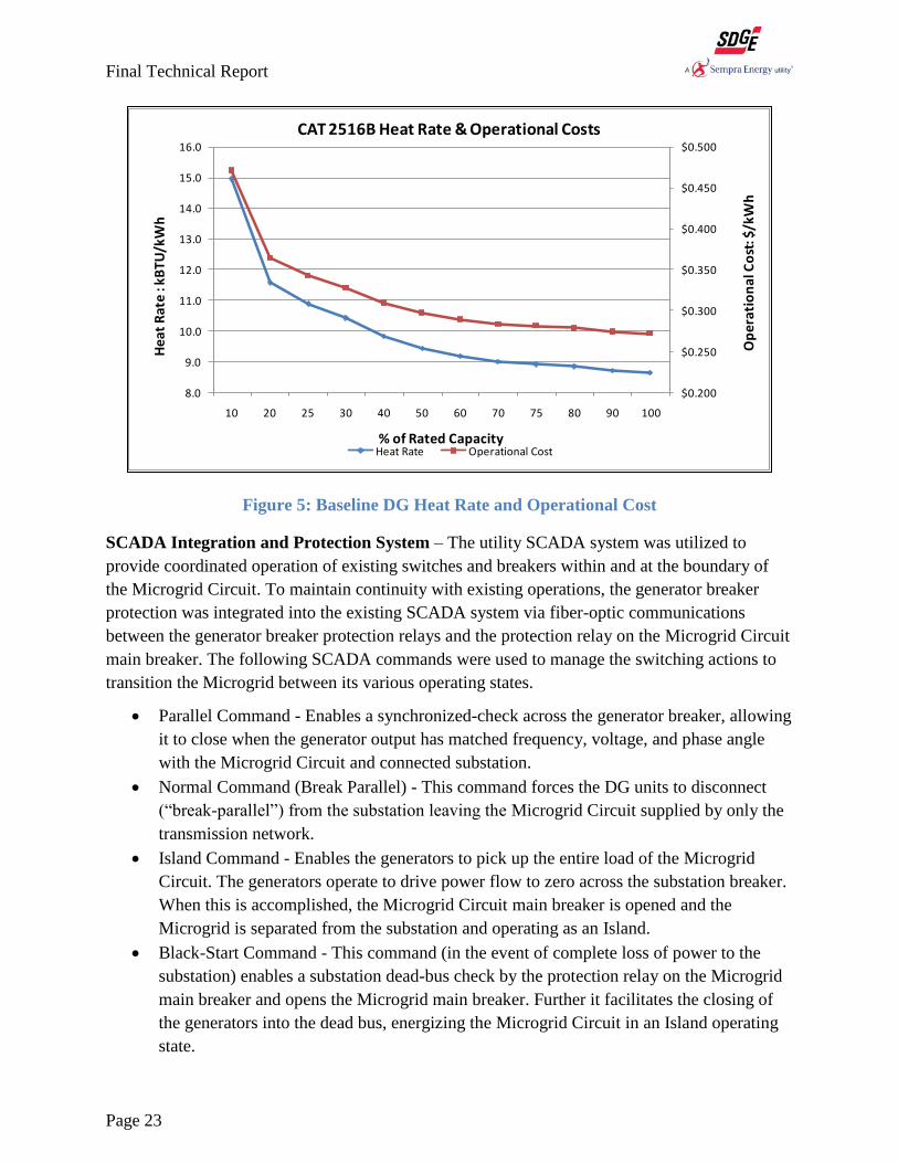
initially detected by the OMS/DMS system the device shows in “Pending State” as shown in
Figure 6.
Final Technical Report
Page 29
Figure 6: New Outage in Pending State
Once the OMS/DMS system confirms the outage through the SCADA interface, the status of the
device displayed in the viewer changes from “Pending” to “RDO” or “Real Device Outage” as
shown in the Viewer window in the foreground of Figure 7. At this point, the SCADA switch at
the Microgrid Grid Circuit Breaker is open in response to a fault in the Microgrid Circuit.
Final Technical Report
Page 30
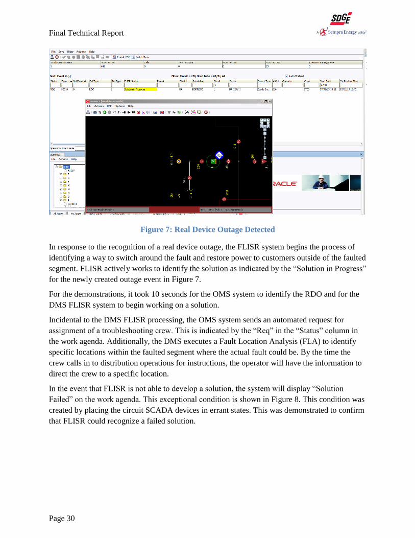
Figure 7: Real Device Outage Detected
In response to the recognition of a real device outage, the FLISR system begins the process of
identifying a way to switch around the fault and restore power to customers outside of the faulted
segment. FLISR actively works to identify the solution as indicated by the “Solution in Progress”
for the newly created outage event in Figure 7.
For the demonstrations, it took 10 seconds for the OMS system to identify the RDO and for the
DMS FLISR system to begin working on a solution.
Incidental to the DMS FLISR processing, the OMS system sends an automated request for
assignment of a troubleshooting crew. This is indicated by the “Req” in the “Status” column in
the work agenda. Additionally, the DMS executes a Fault Location Analysis (FLA) to identify
specific locations within the faulted segment where the actual fault could be. By the time the
crew calls in to distribution operations for instructions, the operator will have the information to
direct the crew to a specific location.
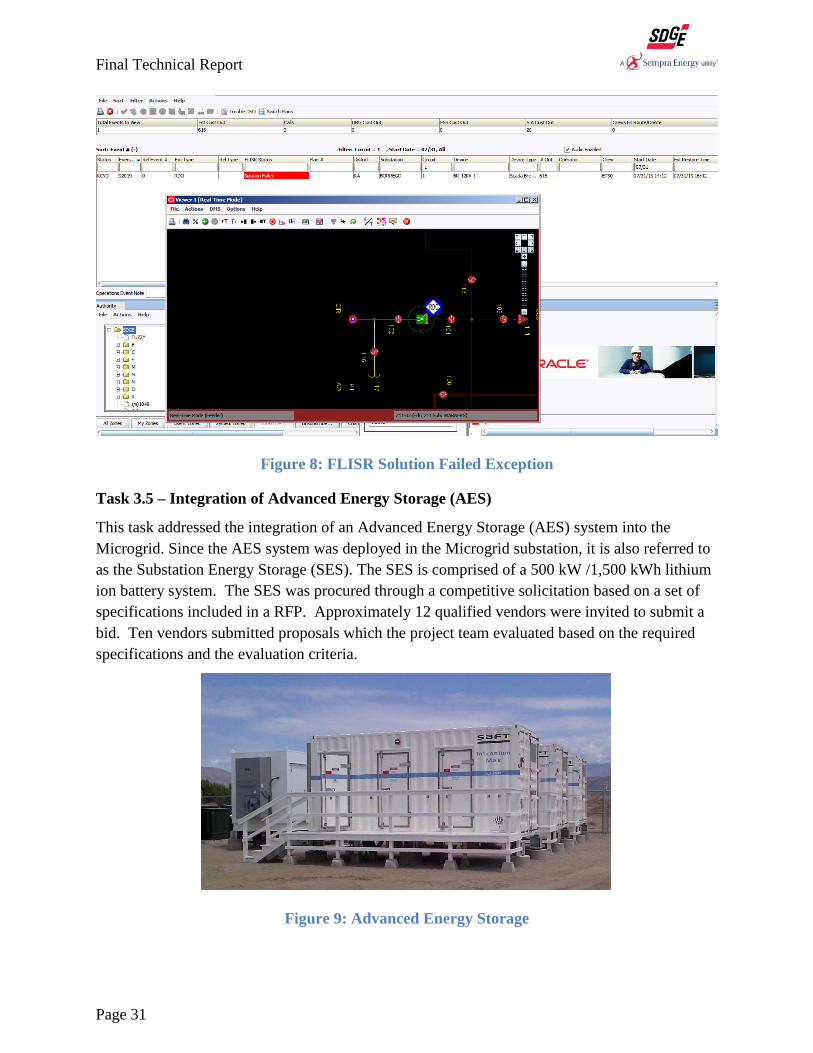
In the event that FLISR is not able to develop a solution, the system will display “Solution
Failed” on the work agenda. This exceptional condition is shown in Figure 8. This condition was
created by placing the circuit SCADA devices in errant states. This was demonstrated to confirm
that FLISR could recognize a failed solution.
Final Technical Report
Page 31
Figure 8: FLISR Solution Failed Exception
Task 3.5 – Integration of Advanced Energy Storage (AES)
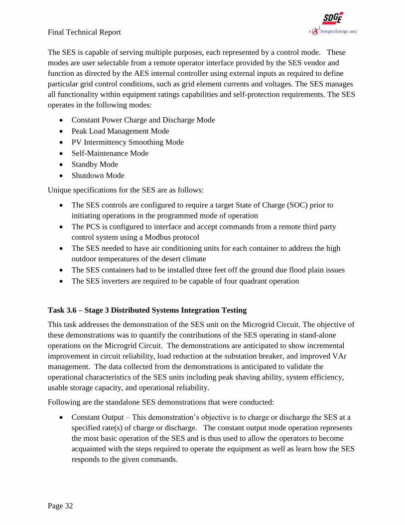
This task addressed the integration of an Advanced Energy Storage (AES) system into the
Microgrid. Since the AES system was deployed in the Microgrid substation, it is also referred to
as the Substation Energy Storage (SES). The SES is comprised of a 500 kW /1,500 kWh lithium
ion battery system. The SES was procured through a competitive solicitation based on a set of
specifications included in a RFP. Approximately 12 qualified vendors were invited to submit a
bid. Ten vendors submitted proposals which the project team evaluated based on the required
specifications and the evaluation criteria.
Figure 9: Advanced Energy Storage
Final Technical Report
Page 32
The SES is capable of serving multiple purposes, each represented by a control mode. These
modes are user selectable from a remote operator interface provided by the SES vendor and
function as directed by the AES internal controller using external inputs as required to define
particular grid control conditions, such as grid element currents and voltages. The SES manages
all functionality within equipment ratings capabilities and self-protection requirements. The SES
operates in the following modes:
Constant Power Charge and Discharge Mode
Peak Load Management Mode
PV Intermittency Smoothing Mode
Self-Maintenance Mode
Standby Mode
Shutdown Mode
Unique specifications for the SES are as follows:
The SES controls are configured to require a target State of Charge (SOC) prior to
initiating operations in the programmed mode of operation
The PCS is configured to interface and accept commands from a remote third party
control system using a Modbus protocol
The SES needed to have air conditioning units for each container to address the high
outdoor temperatures of the desert climate
The SES containers had to be installed three feet off the ground due flood plain issues
The SES inverters are required to be capable of four quadrant operation
Task 3.6 – Stage 3 Distributed Systems Integration Testing
This task addresses the demonstration of the SES unit on the Microgrid Circuit. The objective of
these demonstrations was to quantify the contributions of the SES operating in stand-alone
operations on the Microgrid Circuit. The demonstrations are anticipated to show incremental
improvement in circuit reliability, load reduction at the substation breaker, and improved VAr
management. The data collected from the demonstrations is anticipated to validate the
operational characteristics of the SES units including peak shaving ability, system efficiency,
usable storage capacity, and operational reliability.
Following are the standalone SES demonstrations that were conducted:
Constant Output – This demonstration’s objective is to charge or discharge the SES at a
specified rate(s) of charge or discharge. The constant output mode operation represents
the most basic operation of the SES and is thus used to allow the operators to become
acquainted with the steps required to operate the equipment as well as learn how the SES
responds to the given commands.

Final Technical Report
Page 33
Peak Shave – In this mode of operation, the SES supports an overall project goal to meet
a 15% or greater peak load reduction. SES is not designed to meet this goal by itself but
to contribute to meeting it in conjunction with other Microgrid Resources. In the Peak
Shave Mode, the SES monitors and follows the load at the Microgrid Circuit Breaker and
supplies an appropriate amount of electricity to meet a load that exceeds the input set
point.
VAr Control - The primary objective of the VAr Mode demonstration was to evaluate the
ability of the SES to provide VAr support to the Microgrid Circuit. In this mode of
operation the SES operates in constant output (kW), while varying it’s VAr output to
affect the reactive power at the Microgrid Circuit Breaker.
Arbitrage – The objective of the Arbitrage Mode demonstrations was to test the ability to
dispatch the SES charge and discharge operations in response to the CAISO nodal cost of
electricity. For these demonstrations the SES units were charged during lower CAISO
wholesale prices and discharged during higher CAISO wholesale prices
Four Quadrant Operation - The objective of this demonstration was to observe the
performance of the SES unit in the four quadrants of the power circle by operating the
SES at multiple real power (kW) and reactive power (kVAr) settings. During this set of
operations, the SES unit was set to various real power and reactive power settings
consistent with the manufacturer’s kVA (apparent power) rating of the unit.
Efficiency Demonstration - These demonstration’s evaluated the efficiency and total
storage capacity of the SES system. Efficiency is evaluated based on the AC-AC round
trip operation that is based on energy discharged from the system versus the electricity
that goes into the battery to during the charging process.
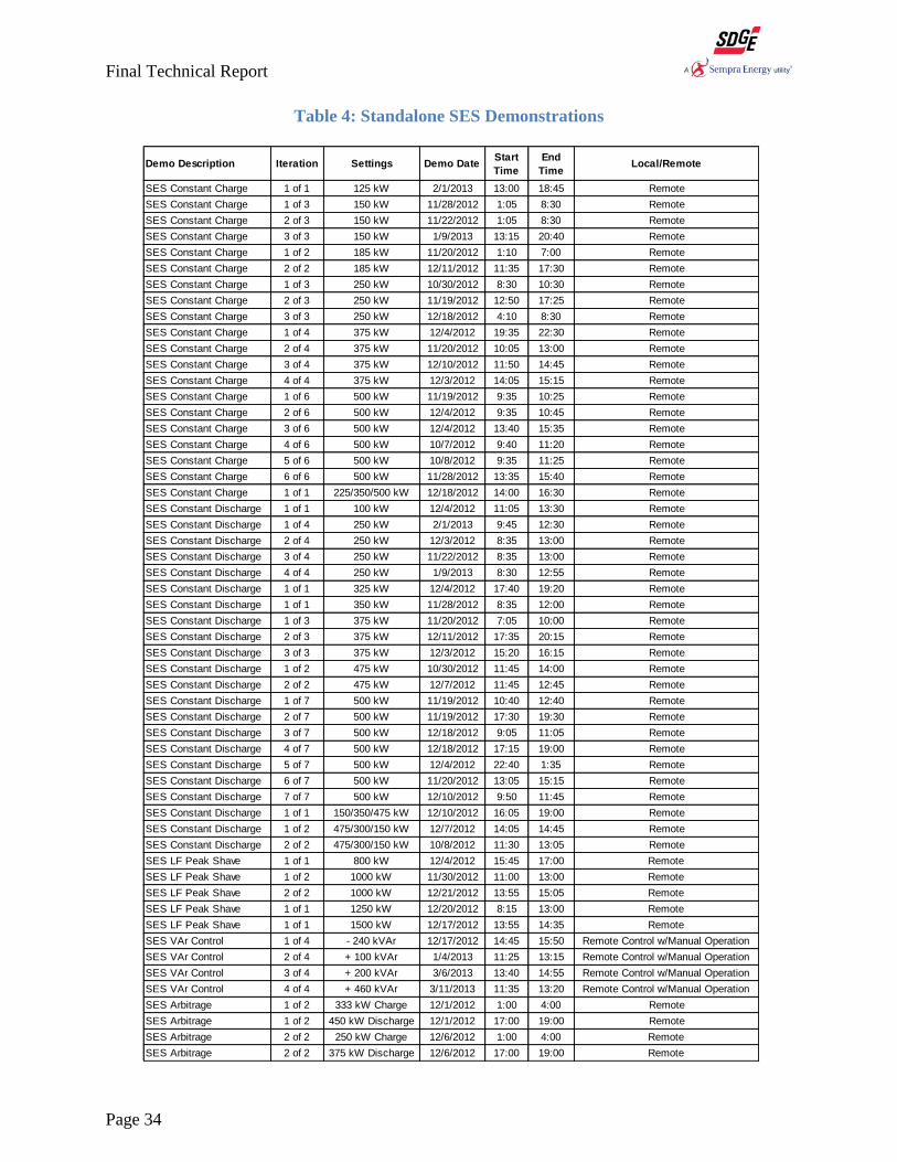
Table 4 presents a comprehensive summary of all the AES stand-alone demonstrations
conducted. The data identifies the description of the demonstration, the set points of the SES
unit, the date, the start time, end time, and control method (local controls or remotely controlled).
Remotely controlled operations were conducted through the Microgrid Visualizer. The table also
shows that demonstrations were conducted several times and the specific iteration is identified.
A total of 55 SES standalone demonstrations were conducted between October 2012 and March
2013.
Final Technical Report
Page 34
Table 4: Standalone SES Demonstrations
Demo Description Iteration Settings Demo DateStart
Time
End
TimeLocal/Remote
SES Constant Charge 1 of 1 125 kW 2/1/2013 13:00 18:45 Remote
SES Constant Charge 1 of 3 150 kW 11/28/2012 1:05 8:30 Remote
SES Constant Charge 2 of 3 150 kW 11/22/2012 1:05 8:30 Remote
SES Constant Charge 3 of 3 150 kW 1/9/2013 13:15 20:40 Remote
SES Constant Charge 1 of 2 185 kW 11/20/2012 1:10 7:00 Remote
SES Constant Charge 2 of 2 185 kW 12/11/2012 11:35 17:30 Remote
SES Constant Charge 1 of 3 250 kW 10/30/2012 8:30 10:30 Remote
SES Constant Charge 2 of 3 250 kW 11/19/2012 12:50 17:25 Remote
SES Constant Charge 3 of 3 250 kW 12/18/2012 4:10 8:30 Remote
SES Constant Charge 1 of 4 375 kW 12/4/2012 19:35 22:30 Remote
SES Constant Charge 2 of 4 375 kW 11/20/2012 10:05 13:00 Remote
SES Constant Charge 3 of 4 375 kW 12/10/2012 11:50 14:45 Remote
SES Constant Charge 4 of 4 375 kW 12/3/2012 14:05 15:15 Remote
SES Constant Charge 1 of 6 500 kW 11/19/2012 9:35 10:25 Remote
SES Constant Charge 2 of 6 500 kW 12/4/2012 9:35 10:45 Remote
SES Constant Charge 3 of 6 500 kW 12/4/2012 13:40 15:35 Remote
SES Constant Charge 4 of 6 500 kW 10/7/2012 9:40 11:20 Remote
SES Constant Charge 5 of 6 500 kW 10/8/2012 9:35 11:25 Remote
SES Constant Charge 6 of 6 500 kW 11/28/2012 13:35 15:40 Remote
SES Constant Charge 1 of 1 225/350/500 kW 12/18/2012 14:00 16:30 Remote
SES Constant Discharge 1 of 1 100 kW 12/4/2012 11:05 13:30 Remote
SES Constant Discharge 1 of 4 250 kW 2/1/2013 9:45 12:30 Remote
SES Constant Discharge 2 of 4 250 kW 12/3/2012 8:35 13:00 Remote
SES Constant Discharge 3 of 4 250 kW 11/22/2012 8:35 13:00 Remote
SES Constant Discharge 4 of 4 250 kW 1/9/2013 8:30 12:55 Remote
SES Constant Discharge 1 of 1 325 kW 12/4/2012 17:40 19:20 Remote
SES Constant Discharge 1 of 1 350 kW 11/28/2012 8:35 12:00 Remote
SES Constant Discharge 1 of 3 375 kW 11/20/2012 7:05 10:00 Remote
SES Constant Discharge 2 of 3 375 kW 12/11/2012 17:35 20:15 Remote
SES Constant Discharge 3 of 3 375 kW 12/3/2012 15:20 16:15 Remote
SES Constant Discharge 1 of 2 475 kW 10/30/2012 11:45 14:00 Remote
SES Constant Discharge 2 of 2 475 kW 12/7/2012 11:45 12:45 Remote
SES Constant Discharge 1 of 7 500 kW 11/19/2012 10:40 12:40 Remote
SES Constant Discharge 2 of 7 500 kW 11/19/2012 17:30 19:30 Remote
SES Constant Discharge 3 of 7 500 kW 12/18/2012 9:05 11:05 Remote
SES Constant Discharge 4 of 7 500 kW 12/18/2012 17:15 19:00 Remote
SES Constant Discharge 5 of 7 500 kW 12/4/2012 22:40 1:35 Remote
SES Constant Discharge 6 of 7 500 kW 11/20/2012 13:05 15:15 Remote
SES Constant Discharge 7 of 7 500 kW 12/10/2012 9:50 11:45 Remote
SES Constant Discharge 1 of 1 150/350/475 kW 12/10/2012 16:05 19:00 Remote
SES Constant Discharge 1 of 2 475/300/150 kW 12/7/2012 14:05 14:45 Remote
SES Constant Discharge 2 of 2 475/300/150 kW 10/8/2012 11:30 13:05 Remote
SES LF Peak Shave 1 of 1 800 kW 12/4/2012 15:45 17:00 Remote
SES LF Peak Shave 1 of 2 1000 kW 11/30/2012 11:00 13:00 Remote
SES LF Peak Shave 2 of 2 1000 kW 12/21/2012 13:55 15:05 Remote
SES LF Peak Shave 1 of 1 1250 kW 12/20/2012 8:15 13:00 Remote
SES LF Peak Shave 1 of 1 1500 kW 12/17/2012 13:55 14:35 Remote
SES VAr Control 1 of 4 - 240 kVAr 12/17/2012 14:45 15:50 Remote Control w/Manual Operation
SES VAr Control 2 of 4 + 100 kVAr 1/4/2013 11:25 13:15 Remote Control w/Manual Operation
SES VAr Control 3 of 4 + 200 kVAr 3/6/2013 13:40 14:55 Remote Control w/Manual Operation
SES VAr Control 4 of 4 + 460 kVAr 3/11/2013 11:35 13:20 Remote Control w/Manual Operation
SES Arbitrage 1 of 2 333 kW Charge 12/1/2012 1:00 4:00 Remote
SES Arbitrage 1 of 2 450 kW Discharge 12/1/2012 17:00 19:00 Remote
SES Arbitrage 2 of 2 250 kW Charge 12/6/2012 1:00 4:00 Remote
SES Arbitrage 2 of 2 375 kW Discharge 12/6/2012 17:00 19:00 Remote

Final Technical Report
Page 35
Task 3.7 – Integration of Outage Management System/Distribution Management System
for Microgrid Operations
The Microgrid Operator is the point of contact to oversee and manage the control and monitoring
functions for the Microgrid. To support the operation, the Microgrid Operator needs to tools to
support the scheduling and operations of the Microgrid Resources. The major activities of the
Microgrid operator include:
Develop a daily load forecast
Collect the appropriate day ahead CAISO Wholesale Price and input into the Microgrid
pricing model
Schedule Microgrid Resources to optimize Microgrid operations
Create DR Event Trigger within the PDLM System as needed
Schedule DR Resources within the PDLM System
The tools and system integrations that are required to facilitate these activities are a consolidated
control interface, a load forecast model, and a resource pricing model.
Consolidated Control Interface
During the Microgrid design stage, it was envisioned that an external vendor would be added to
the Project Team to develop the Microgrid Controller. The team worked with a third party
vendor to develop system functional requirements and an integration plan for a Microgrid
Controller until it became clear that the planned approach was not able to be executed in the
required time frame. The Project Team decided to use in-house tools to develop a system
(Microgrid Visualizer) that could support the Microgrid operations required to execute the
Project Demonstration Plans. This tool was used as the integration point that provides the
interface between the Microgrid resources and various SDG&E systems of the DMS, SCADA
and Microgrid Operational Database.
The Microgrid Visualizer is a custom developed solution deployed on an OSI PI Asset
Framework. Figure 10 presents a high level architecture for the Visualizer identifying
infrastructure required at the Microgrid Site, a utility data center and the Microgrid Operator’s
office. The system communicates with the Microgrid Resources via a pair of gateways; one
located in the data center and the other located in the Microgrid Yard with all resources within
the Utility’s secure network.

Final Technical Report
Page 36
Figure 10: High Level Visualizer Architecture
The Microgrid Visualizer was created using PI Process Book to act as the user interface. The
Microgrid Operator can access the Visualizer from the Control Van located within the Microgrid
Yard or remotely from SDG&E’s offices in San Diego. The Visualizer user interface is presented
in Figure 11 with key monitoring and control components for the critical SCADA switches,
circuit load, each of the DG units, SES system, and system alarms.
Borrego Gateway MPK Gateway Desktop/Visualizer
PI Server
GEN #1
PI Server
Borrego DataCenter Office
GEN #2
SES
DEM (CES)
Profile Scheduler (Excel)
Data Warehouse (PI System Explorer)

Final Technical Report
Page 37
Figure 11: PI Process Book HMI Screen Design – Manual Mode Screen
The Visualizer provides the Microgrid Operator the option of operating the equipment in a
manual mode or in a scheduled mode. The system is configured to continuously collect system
data and store it in a PI database. Data can be easily extracted for analysis and reporting using a
PI add-in for Excel.
Load Forecast Model
Several regression models were tested as the forecast model. Variations models showed that the
air temperature is the most significant driver of the load during the daytime but not at night. The
dew point and relative humidity did not add significantly to the accuracy of any of the tested
models. The unique shape of the Microgrid Circuit load profile is attributed to high night-time
loads from pumping operation by the water district and agricultural customers on the circuit.
This phenomenon led to the inclusion of a “Pump Schedule Flag” in the model to account for the
load shift resulting from time-of-use pricing incentives and highly elastic temporal energy
demands. The best fit model was based on the following variables:
Time of Day (Military format with no colon)
Air Temperature (oF)
Pump Schedule Flag ( 1’s and 0’s, set to 1 from 11:00 PM to 5:00 AM)

Final Technical Report
Page 38
Average of three previous weekday’s load at the same time day (MW)
Average of three previous weekday’s temperatures at the same time (oF)
Forecast Load (MW) =
(Time x .000028) + (Pump Flag x .6719) + (Temp Forecast x .0339) +
(3day Avg. Temp x -.0317) + (3day Avg. Load x .6029) + .460
Pricing Model
The Pricing Module was used to calculate the wholesale price of electricity ($/MWh) for
electricity delivered to customers within the Microgrid. The wholesale price is dependent on the
operation of Microgrid Resources along with the transmission grid. If the Microgrid resources
are non-operational, the wholesale price is equal to the Locational Marginal Price (LMP) at the
Borrego node. This LMP nodal price is obtained through an interface with CAISO’s Nodal LMP
system (referred to as OASIS). If the Microgrid resources are operational, the wholesale price is
calculated by calculating an average weighted price of energy obtained from the grid at the LMP
nodal price and the price of energy produced by the operating Microgrid Resources.
The wholesale price consists of the following components:
DG# 1 Price – Price associated with the operation of Distributed Generator # 1
DG# 2 Price – Price associated with the operation of Distributed Generator # 2
Grid Price - The Grid Price is equal to the CAISO DAM LMP price for the Borrego Node
SES Price – Price associated with the charge/discharge operation of the Substation
Energy Storage unit
CAISO wholesale prices were downloaded from the CAISO OASIS website on a daily basis.
The data was available in a comma separated values file and was transferred to the Microgrid
Visualizer. An internal script running on the Microgrid Visualizer picked up the CAISO price
and transferred the values to the Pricing Module once every 24-hours.
The base formula to calculate the Total Weighted Average Price (𝑀𝑖𝑐𝑟𝑜𝑔𝑟𝑖𝑑 𝑃𝑟𝑖𝑐𝑒$/𝑀𝑊ℎ) is:
(𝑀𝑊𝐷𝐺1 ∗ $
𝑀𝑊𝐻𝐷𝐺1) + (𝑀𝑊𝐷𝐺2 ∗
$
𝑀𝑊𝐻𝐷𝐺2) + (𝑀𝑊𝑆𝐸𝑆 ∗
$
𝑀𝑊𝐻𝑆𝐸𝑆) + (𝑀𝑊𝐺𝑅𝐼𝐷 ∗
$
𝑀𝑊𝐻𝐺𝑅𝐼𝐷)
𝑀𝑊𝐷𝐺1 + 𝑀𝑊𝐷𝐺2 + 𝑀𝑊𝑆𝐸𝑆 + 𝑀𝑊𝐺𝑅𝐼𝐷
An exception to this calculation occurs when the SES is in the charging mode. The Total
Weighted Average Price (𝑀𝑖𝑐𝑟𝑜𝑔𝑟𝑖𝑑 𝑃𝑟𝑖𝑐𝑒$/𝑀𝑊ℎ) during the charging interval is calculated by
excluding the SES Aggregate Price component. The value of electricity in the SES unit is
accounted for by using the LMP price at the time of the charging and the quantity of electricity
added to the SES while charging. Prior to discharging the SES unit, the average cost of
electricity for all the energy stored in the unit is calculated. This is used as the basis of the price
of energy from the SES unit during the entire discharge cycle

Final Technical Report
Page 39
Task 3.8 – Stage 4 Distributed Systems Integration Testing
The Microgrid Visualizer developed as part of this project was utilized as a core tool for remote
operation of the Microgrid Resources during a majority of the demonstrations. The Visualizer
was an important integration point to various utility systems like the OMS/DMS, SCADA
system and the PDLM system. This tool was effectively used by Microgrid Operators to monitor
and schedule the resources for operation in various modes to support Microgrid operations. The
Visualizer required several external inputs to be loaded into the system manually. The
Visualizer met the needs of the project to support planned demonstrations but is not sufficient to
act as a standalone Microgrid Controller.
Figure 12 presents the Visualizer user interface when a scheduled operation is being executed.
This interface provides the Microgrid Operator with the status and operating parameters of each
of the Microgrid Resources as well as the scheduled operation. This provides feedback to the
Operator whether or not the Microgrid is operating as anticipated.
Figure 12: Microgrid Visualizer User Interface
The Load Forecast integrates with the Microgrid Visualizer to provide detail insight into the
expected load over a 24-hour period and provides the ability to schedule resources on day-ahead
schedule. The load forecast model was not as accurate or precise as hoped but was an effective
tool to provide an estimate of timing and magnitude of peaks and well as validating the ability
for Microgrid Resources to meet the anticipated Microgrid Circuit load during planned
demonstration operations.

Final Technical Report
Page 40
The Pricing Module was used effectively to translate the cost of operating Microgrid Resources
as a wholesale price that could be passed on to the PDLM system to trigger pricing events. The
Pricing Model was also used to try to operate a combination of Microgrid Resources in a cost-
effective manner. This included influencing the timing and rates to charge and discharge the
SES unit as well as selecting operating set points for the DG units.
Task 3.9 – Integration of Price-Driven Load Management
This task addresses the development and integration of a Price-Driven Load Management
(PDLM) system for managing customer load on the Microgrid. The PDLM system dispatches the
customer-side of the meter resources. The PDLM system interfaces with SDG&E’s existing AMI
system, project supplied Home Area Network (HAN) systems, and the Residential Energy
Storage systems through the PDLM controller. Customer-side technologies that integrate into
the PDLM system are:
Programmable Communicating Thermostat (PCT)
Load Control Switch (LCS)
Plug Load Controller (PLC)
In-Home Display (IHD)
Residential Energy Storage
Customer Web Portal
The PDLM controller is the system of record to forecast Demand Response (DR) capacity and
schedule DR events to meet the load reduction objectives within the Microgrid. Figure 13 on the
following page describes the PDLM architecture deployed in the Microgrid demonstration
project.

Final Technical Report
Page 41
Figure 13: High Level PDLM Architecture
PDLM Controller - The PDLM controller functionality includes:
Demand Response through Direct Load Control and Dynamic Pricing signals.
Forecast Demand Response on a rolling 48-hour basis
Monitor and execute Demand Response events
Post-event measurement & verification (M&V)
Analyze historical Demand Response data
The PDLM system enables operators to:
Create and manage various types of Demand Response programs (i.e. Direct Load
Control programs, Dynamic Pricing Program, etc.)
Facilitate customer enrolment and notification of DR events, through its interface with
the HAN System
Initiate DR signals to be sent to the HAN devices through the HAN NOC
Capture post event information for billing and inventive purposes
Monitor and control the Residential Energy Storage system.
Figure 14 on the following page provides a snapshot of the utility portal that enables operators to
perform the required Demand Response functions.
Residential Energy
Storage Unit
HAN
Devices
Customer
Meter Data
Connect
(NOC)
HAN System
IHD
LCS
Gateway
ZigBee with Smart
Energy Profile
Web Services or API callEDIX
HTTPs
PDLM
DB Server
Broadband
MDMS
Microgrid
Controller
CAISO
Price Feed
NOAA
Weather
Feed
CIS/
GIS
Operator
SDG&E NOC
Customer
Internet
Gateway
Smart
Meter
.
Amazon Cloud
PLCResidential Energy Storage NOC
(Cloud Based)
Customer Premises – Borrego Springs
PCT
PDLM
Controller

Final Technical Report
Page 42
Figure 14: PDLM System Utility Portal
HAN System - The HAN Network Operations Center (NOC) manages HAN devices installed in
customer premises. The devices are configured to control loads based on event-based activities
demand response and price-based activities. The HAN system consists of a gateway that
communicates with the in home devices (through wireless control signals) such as the in-home
display, programmable communicating thermostats, load control switches, and plug load
controllers. The end devices are configured to control loads based on event-based activities (i.e.
demand response events) or price-based activities. Figure 15 shows a typical system
configuration with the HAN devices installed in customer homes.
Figure 15: Typical Customer HAN Device Configuration
IHD
PCTLCS
PLC
Gateway
Smart Meter
Internet Router

Final Technical Report
Page 43
Task 3.10 – Stage 5 Distributed Systems Integration Testing
This task documents the PDLM demonstrations performed as part of the Microgrid
demonstration. These operations were planned as Standalone PDLM demonstrations that were
carried out to support the overall objectives in support of Microgrid operations. The PDLM
demonstrations were conducted in two phases.
Phase 1 – Standard DR Demonstrations- The first phase of PDLM demonstration involved
standard demand reduction programs. In standard DR events, the customer was enrolled in one
or more demand reduction programs that would be planned a day in advance. During this phase,
customers had the choice to participate or to opt out of any specific event. The following types of
direct load control programs were developed (within the PDLM Controller) to meet the
objectives of demonstrating Traditional Demand Response.
PCT Program - The PDLM system sends a command to the program enrollee’s PCT to
modify the temperature set point. It supports multiple levels of temperature offset, as per
customer preference.
PLC Program - The PDLM system sends a command to the PLC which is connected to
consumer devices like fans, lamps, televisions and other in-home devices. The PLC
disconnects power to the consumer device during an event providing the anticipated
reduction in load.
Table 5 presents information on the post event analysis provided by the PDLM controller for the
Standard DR tests conducted between December 2012 and February 2013. The PDLM
Controller’s Analysis module provides the post-event analysis. It utilizes the configured DR
Programs to execute DR events based on program constraints and restrictions. The DR Capacity
Forecast is a learning algorithm that converges on the measured results each time a DR event is
executed and accounts in the post event analysis. The results of the DR event are fed back into
the DR Capacity Forecast.

Final Technical Report
Page 44
Table 5: DR Events Demonstration Summary
Date Start
Time
End
Time
Du
rati
on
Ty
pe
of
DR
Pro
gra
m
Pre
dic
ted
Lo
ad
Red
uct
ion
(k
W)
Act
ua
l L
oa
d
Red
uct
ion
(k
W)
Sch
edu
led
Pa
rtic
ipa
nts
Sch
edu
led
Dev
ices
Dev
ices
Op
ted
Ou
t
Per
cen
t D
evic
e
Pa
rtic
ipa
tio
n
Per
cen
t D
evic
e
Op
t O
ut
12/13/12 14:00 15:00 1:00 PLC 418.50 (3.39) 50 91 8 91.2% 8.8%
12/14/12 14:00 15:00 1:00 PLC 38.50 (3.48) 50 91 8 91.2% 8.8%
12/18/12 14:00 15:00 1:00 PLC 38.40 (1.59) 50 91 8 91.2% 8.8%
12/20/12 15:00 16:00 1:00 PLC 42.60 (6.64) 35 45 7 84.4% 15.6%
1/8/13 14:00 15:00 1:00 4 ⁰F Offset 12.70 7.67 47 58 0 100.0% 0.0%
1/8/13 14:00 15:00 1:00 PLC 37.90 9.82 50 91 7 92.3% 7.7%
1/8/13 15:00 16:00 1:00 4 ⁰F Offset 19.10 12.70 47 58 0 100.0% 0.0%
1/8/13 15:00 16:00 1:00 PLC 42.20 13.24 50 91 7 92.3% 7.7%
1/17/13 14:00 15:00 1:00 PLC 4.10 1.02 50 91 6 93.4% 6.6%
1/17/13 15:00 16:00 1:00 PLC 19.10 3.68 50 91 6 93.4% 6.6%
1/22/13 14:00 15:00 1:00 PLC,
4 ⁰F Offset
20.80 11.77 51 149 6 96.0% 4.0%
1/22/13 15:00 16:00 1:00 PLC,
4 ⁰F Offset
35.90 7.83 51 149 6 96.0% 4.0%
1/24/13 15:00 16:00 1:00 PLC,
4 ⁰F Offset
31.80 1.11 51 149 6 96.0% 4.0%
1/29/13 14:00 15:00 1:00 PLC 4.10 1.77 36 45 5 88.9% 11.1%
1/29/13 14:00 15:00 1:00 PLC 1.50 8.91 36 46 4 91.3% 8.7%
1/29/13 15:00 16:00 1:00 PLC 19.20 0.67 36 45 5 88.9% 11.1%
1/29/13 15:00 16:00 1:00 PLC 11.00 5.90 36 46 4 91.3% 8.7%
1/29/13 16:00 17:00 1:00 PLC 0.00 4.47 36 45 5 88.9% 11.1%
1/31/13 14:00 15:00 1:00 4 ⁰F Offset 16.80 9.35 47 58 0 100.0% 0.0%
1/31/13 14:00 15:00 1:00 PLC 1.50 8.09 36 46 0 100.0% 0.0%
1/31/13 14:00 15:00 1:00 PLC 4.10 5.11 36 45 5 88.9% 11.1%
1/31/13 15:00 16:00 1:00 4 ⁰F Offset 12.60 12.06 47 58 0 100.0% 0.0%
1/31/13 15:00 16:00 1:00 PLC 11.00 8.43 36 46 0 100.0% 0.0%
1/31/13 15:00 16:00 1:00 PLC 19.20 7.05 36 45 5 88.9% 11.1%
2/5/13 15:00 16:00 1:00 PLC 36.10 4.46 51 149 5 96.6% 3.4%
2/13/13 14:00 15:00 1:00 PLC 4.10 8.92 50 91 4 95.6% 4.4%
2/13/13 15:00 16:00 1:00 PLC 19.30 12.30 50 91 4 95.6% 4.4%
2/14/13 14:00 15:00 1:00 PLC 4.10 0.79 50 91 0 100.0% 0.0%
2/14/13 14:00 15:00 1:00 4 ⁰F Offset 16.90 (2.08) 47 58 0 100.0% 0.0%
2/14/13 15:00 16:00 1:00 PLC 19.30 9.85 50 91 0 100.0% 0.0%
2/14/13 15:00 16:00 1:00 4 ⁰F Offset 12.70 6.87 47 58 0 100.0% 0.0%
2/14/13 16:00 17:00 1:00 PLC 0.00 5.23 50 91 0 100.0% 0.0%
2/14/13 16:00 17:00 1:00 4 ⁰F Offset 0.00 4.46 47 58 0 100.0% 0.0%
2/19/13 14:00 15:00 1:00 PLC 4.10 11.98 50 91 5 94.5% 5.5%
2/19/13 15:00 16:00 1:00 PLC 19.40 8.05 50 91 5 94.5% 5.5%
2/21/13 14:00 15:00 1:00 PLC 4.10 6.40 50 91 5 94.5% 5.5%
2/21/13 15:00 16:00 1:00 PLC 19.40 (4.47) 50 91 5 94.5% 5.5%
2/21/13 16:00 17:00 1:00 PLC 0.00 (3.82) 50 91 5 94.5% 5.5%
2/26/13 14:00 15:00 1:00 PLC 4.10 2.46 50 91 4 95.6% 4.4%
2/26/13 14:00 15:00 1:00 4 ⁰F Offset 4.20 (6.31) 47 58 0 100.0% 0.0%
2/26/13 15:00 16:00 1:00 PLC 19.50 (0.81) 50 91 4 95.6% 4.4%
2/26/13 15:00 16:00 1:00 4 ⁰F Offset 0.00 (3.24) 47 58 0 100.0% 0.0%

Final Technical Report
Page 45
Data from Table 5 was analyzed to understand the effect of Demand Response on customer load
reduction. Between December 2012 and February 2013, a total of 42 Demand Response events
were implemented. Each DR event was scheduled for 1 hour, while some days had multiple DR
events. Out of the 42 DR events, 32 DR events registered a net reduction in customer load, while
10 DR events registered a net increase in customer load. This analysis shows that 76% of the
time a net reduction in customer load was observed, while 24% of the time a net increase in
customer load was observed. During the 32 DR events in which a load reduction was observed,
the average total load reduction was 7.0 kW. During the 10 DR events in which a load increase
was observed, the average total load increase was 3.6 kW. The average total change in load
across all 42 DR events was a total load reduction of 4.4 kW. A summary of the event analysis
for the DR events conducted between December 2012 and February 2012 is presented in Table 6.
Table 6: DR Events Load Reduction Summary
Number of DR Event Days 16 Days
Number of DR event hours 42 Hours
DR events with Load Reduction 76%
DR events with Load Increase 24%
Average Load Reduction
(when load reduced during DR events) 7.0 kW / event
Average Load Increase
(when load increase during DR events) 3.6 kW / event
Average Load Reduction During all DR
events 4.4 kW
During the initial DR events the predicted load reduction was observed to be higher than the
actual available DR on the Microgrid Circuit. A correction factor was applied to the DR Forecast
algorithm that provided more accuracy to the forecast. Since many of the events have a measured
net increase in load, secondary analysis was conducted to identify specific instances of customers
who reduced their load during the events. Data was collected and analyzed from the HAN NOC.
This data is not typically available to the end user and was requested by the project team. The
process of acquiring the data was not straight forward as the HAN vendor does not typically
store this data. The Vendor had to develop a special case to capture and archive this data for the
team to analyze. As a result of the problems for the vendor to obtain the data and unique nature
of the request, the HAN data was not available for all of the events that were executed.
Since the post event data represents the load impact of the aggregated customer base, further
analysis was performed to understand the effect of DR events on individual customer load
reduction. Hourly customer interval data was obtained from the AMI system for customers that
participated in the DR demonstrations. The data was analyzed to see the trend of customer load
on the days of the event and an average of the customer load over 3-days or 7-days prior to the

Final Technical Report
Page 46
event. This analysis identified several instances of actual load reduction in customer homes
during the DR demonstrations. In absence of the DR events, the customer load would have
remained higher. Figure 16 presents AMI data for a sample customer who participated in the DR
events and had significant load reduction of during the DR events. The chart below presents two
load curves for comparison:
Event Day Load Curve (red line), and
Average Load for Days Prior to Event (black line)
As presented in Figure 16, a two hour DR event was executed between 14:00 and 16:00. The
load of the customer was significantly higher than the average load at the beginning of the event
and was reduced to a level lower than the average during the second hour of the event (to less
than 1.0 kW). The data shows that the customer had an overall load reduction of 4.6 kW during
the event.
Figure 16: Example 1- Customer Load Reduction During DR Events
Phase 2 – Simulating Pricing Demonstrations - The second phase of the PDLM demonstration
was based on triggering demand reduction based on pricing signals that were communicated to
the HAN systems. In these programs, the customer does not have a simple opt out option but
can alter the impact of the event by changing their pricing threshold through the customer portal.
This allows a customer with two Programmable Communicating Thermostats (PCTs), for
example, to have one accept the temperature offset at one price point while the other PCT
participates at a higher price point. The PDLM system transmits simulated wholesale prices
which are translated into retail pricing after taking into consideration the CAISO nodal pricing in
Borrego Springs and the cost of operating Microgrid resources. The customers have the ability to
configure individual in-home devices to respond to a retail price. Thus, the equipment operation
0.0
1.0
2.0
3.0
4.0
5.0
6.0
7.0
8.0
9.0
1:0
0
2:0
0
3:0
0
4:0
0
5:0
0
6:0
0
7:0
0
8:0
0
9:0
0
10
:00
11
:00
12
:00
13
:00
14
:00
15
:00
16
:00
17
:00
18
:00
19
:00
20
:00
21
:00
22
:00
23
:00
0:0
0
De
ma
nd
(kW
)
Time of Day
AMI Data
Event Day Average Load for Days Prior to Event
DR EventDR Event
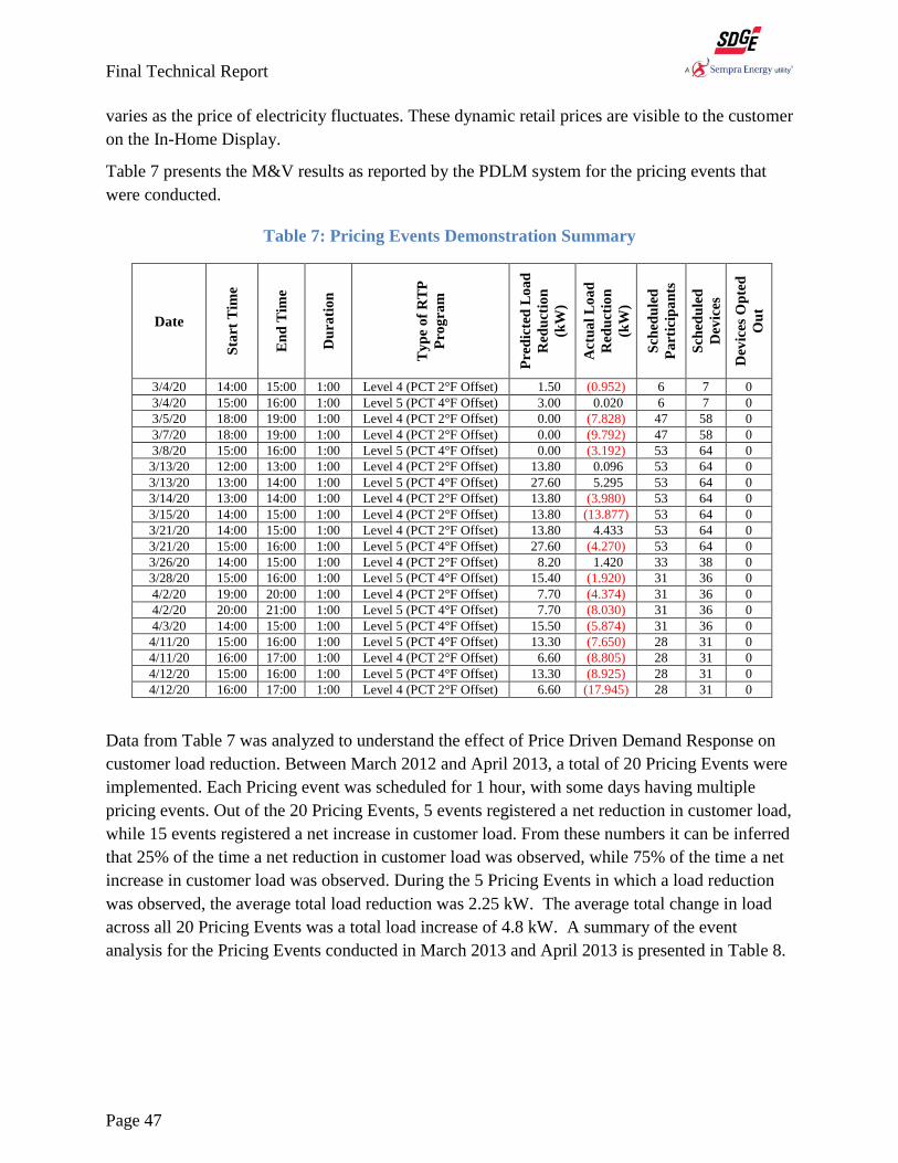
Final Technical Report
Page 47
varies as the price of electricity fluctuates. These dynamic retail prices are visible to the customer
on the In-Home Display.
Table 7 presents the M&V results as reported by the PDLM system for the pricing events that
were conducted.
Table 7: Pricing Events Demonstration Summary
Date
Sta
rt T
ime
En
d T
ime
Du
rati
on
Ty
pe
of
RT
P
Pro
gra
m
Pre
dic
ted
Lo
ad
Red
uct
ion
(kW
)
Act
ua
l L
oa
d
Red
uct
ion
(kW
)
Sch
edu
led
Pa
rtic
ipa
nts
Sch
edu
led
Dev
ices
Dev
ices
Op
ted
Ou
t
3/4/20 14:00 15:00 1:00 Level 4 (PCT 2°F Offset) 1.50 (0.952) 6 7 0
3/4/20 15:00 16:00 1:00 Level 5 (PCT 4°F Offset) 3.00 0.020 6 7 0
3/5/20 18:00 19:00 1:00 Level 4 (PCT 2°F Offset) 0.00 (7.828) 47 58 0
3/7/20 18:00 19:00 1:00 Level 4 (PCT 2°F Offset) 0.00 (9.792) 47 58 0
3/8/20 15:00 16:00 1:00 Level 5 (PCT 4°F Offset) 0.00 (3.192) 53 64 0
3/13/20 12:00 13:00 1:00 Level 4 (PCT 2°F Offset) 13.80 0.096 53 64 0
3/13/20 13:00 14:00 1:00 Level 5 (PCT 4°F Offset) 27.60 5.295 53 64 0
3/14/20 13:00 14:00 1:00 Level 4 (PCT 2°F Offset) 13.80 (3.980) 53 64 0
3/15/20 14:00 15:00 1:00 Level 4 (PCT 2°F Offset) 13.80 (13.877) 53 64 0
3/21/20 14:00 15:00 1:00 Level 4 (PCT 2°F Offset) 13.80 4.433 53 64 0
3/21/20 15:00 16:00 1:00 Level 5 (PCT 4°F Offset) 27.60 (4.270) 53 64 0
3/26/20 14:00 15:00 1:00 Level 4 (PCT 2°F Offset) 8.20 1.420 33 38 0
3/28/20 15:00 16:00 1:00 Level 5 (PCT 4°F Offset) 15.40 (1.920) 31 36 0
4/2/20 19:00 20:00 1:00 Level 4 (PCT 2°F Offset) 7.70 (4.374) 31 36 0
4/2/20 20:00 21:00 1:00 Level 5 (PCT 4°F Offset) 7.70 (8.030) 31 36 0
4/3/20 14:00 15:00 1:00 Level 5 (PCT 4°F Offset) 15.50 (5.874) 31 36 0
4/11/20 15:00 16:00 1:00 Level 5 (PCT 4°F Offset) 13.30 (7.650) 28 31 0
4/11/20 16:00 17:00 1:00 Level 4 (PCT 2°F Offset) 6.60 (8.805) 28 31 0
4/12/20 15:00 16:00 1:00 Level 5 (PCT 4°F Offset) 13.30 (8.925) 28 31 0
4/12/20 16:00 17:00 1:00 Level 4 (PCT 2°F Offset) 6.60 (17.945) 28 31 0
Data from Table 7 was analyzed to understand the effect of Price Driven Demand Response on
customer load reduction. Between March 2012 and April 2013, a total of 20 Pricing Events were
implemented. Each Pricing event was scheduled for 1 hour, with some days having multiple
pricing events. Out of the 20 Pricing Events, 5 events registered a net reduction in customer load,
while 15 events registered a net increase in customer load. From these numbers it can be inferred
that 25% of the time a net reduction in customer load was observed, while 75% of the time a net
increase in customer load was observed. During the 5 Pricing Events in which a load reduction
was observed, the average total load reduction was 2.25 kW. The average total change in load
across all 20 Pricing Events was a total load increase of 4.8 kW. A summary of the event
analysis for the Pricing Events conducted in March 2013 and April 2013 is presented in Table 8.

Final Technical Report
Page 48
Table 8: Pricing Events Load Reduction Summary
Number of RTP event days 14 Days
Number of RTP event hours 20 Hours
RTP events with Load Reduction 25%
RTP events with Load Increase 75%
Average Load Reduction
(when load reduced during RTP
events)
2.25 kW / event
Average Load Increase
(when load increase during RTP
events)
7.16 kW / event
Average Load Increase During all
RTP events 4.8 kW
Since many of the events have a measured net increase in load, secondary analysis was
conducted to identify specific instances of customers who reduced their load during the events.
Data was collected and analyzed from the HAN NOC. This data is not typically available to the
end user and was requested by the project team. The process of acquiring the data was not
straight forward as the HAN vendor does not typically store this data. The Vendor had to
develop a special case to capture the data as requested by the project team. Due to the unique
nature of the request, the HAN data was not available for all of the events that were executed.
The analysis included understanding the effect of Pricing Events on actual customer load
reduction. Hourly customer interval data (kW) was downloaded from the Meter Data
Management System for customers that participated in the Pricing demonstrations. The data was
analyzed to see the trend of customer load on the days of the event and an average of the
customer load over 3-days or 7-days prior to the event.
This analysis helps present instances of actual load reduction in customer homes during the
Pricing Event demonstrations. Figures 16-19 present the load profiles for certain customers who
participated in the Pricing events, and had significant load reduction of during these events. The
charts below present two load curves for comparison:
Event Day Load Curve (red line)
Average Load for Days Prior to Event (black line)
Figure 17 presents an example of a customer load during two consecutive Pricing Events [Level
4 (PCT 2 ºF Offset) and Level 5 (PCT 4 ºF Offset)] that were executed between 14:00 and 16:00.
The data shows a reduction in load during the first hour and then a further decline during the
second hour when the PCT set point was adjusted an additional 2oF. This customer
demonstrated a load reduction of 2.4 kW during the event.

Final Technical Report
Page 49
Figure 17: Example 1- Customer Load Reduction During Pricing Event
A major objective of the demonstration project was to discover how the PDLM resources could
be managed in the Microgrid environment and if PDLM could be managed like the other DER
resources. Ideally, PDLM could be managed in the Microgrid the way that generators or storage
systems are managed.
The PDLM is limited and constrained by the capacity of PDLM to deliver load reduction
depends on weather, time of day, and customer behavior. With PDLM, operations must address
the needs of customers as well and devices and systems. Agreements with customers limit the
frequency and duration of PDLM events. Customers have the option to opt-out of events. The
dependability of PDLM resources can vary with customer fatigue and other uncontrollable
customer behavior.
Finally, the methodology for forecasting demand reduction is largely based on trial and error
with incremental refinement of estimates based on experience. This means that early forecasts
are unlikely to be reliable. It takes considerable refinement over multiple events to develop
reliable estimates. All the issues that impact the PDLM forecasts would be improved by
removing the customers’ freedom of choice. However, for these demonstrations, that was not an
option.
Taken together, PDLM is very different from the other DER resources being managed by the
Microgrid Controller. While it can be dispatched as part of the overall Microgrid Optimized plan,
benefiting from PDLM requires a wider variety of operational considerations and is far less
reliable and predictable than other resources.
0.0
0.5
1.0
1.5
2.0
2.5
3.0
3.5
4.0
4.5
1:0
0
2:0
0
3:0
0
4:0
0
5:0
0
6:0
0
7:0
0
8:0
0
9:0
0
10
:00
11
:00
12
:00
13
:00
14
:00
15
:00
16
:00
17
:00
18
:00
19
:00
20
:00
21
:00
22
:00
23
:00
0:0
0
De
ma
nd
(kW
)
Time of Day
AMI Data
Event Day Average Load for Days Prior to Event
RTP Event RTP Event

Final Technical Report
Page 50
Task 3.11 – Feeder Optimization Testing
Task 3.11 builds on Distributed Systems Testing undertaken in Tasks 3.2, 3.4 and 3.6 to integrate
various Microgrid resources and operate them to achieve optimization operation of the Microgrid
Circuit and the Microgrid Resources. The objective of this task is to operate the Microgrid
utilizing the combination of resources in a manner that achieves a 15% or greater peak load
reduction, increases reliability and operates in a cost-effective manner. This will be achieved
through the use of the load forecast tool, CAISO pricing signals, the Microgrid Visualizer and
the sequence of operation of the Microgrid Resources. The key optimization activities address
the following operating scenarios:
Distributed Energy Resource and Substation Energy Storage sequence of operation
Peak Shave operation (Reducing night time peak load)
VAr Operation with DG and SES
Microgrid Island Operation
These demonstrations validated the objective of achieving 15% peak load reduction on the
Microgrid Circuit by simultaneous operation of the Microgrid resources. The sequence of
operations required to operate the Microgrid resources under these scenarios provides valuable
operational information that can be used for future Microgrid operations. The Microgrid
resources can be planned for combined operation based on the load forecast, and are able to react
to changes in load on the circuit by operating at modified set points. The findings from the
various demonstrations can be summarized below:
The constant output demonstrations show that while the resources were able to operate in
individual constant output modes, they were also able to operate simultaneously. The
operation DG and SES was able to meet a higher percentage of the load on the circuit,
thereby reducing the power imported from the grid. The demonstrations identified that
the SES could operate in both charge and discharge modes and rates of energy transfer
without adversely affecting the DG operation.
The peak shave demonstrations show that the Microgrid resources (DG and SES) could
be effectively used to reduce the peak load on the circuit. An important objective of the
overall Microgrid project was demonstrated effectively, when the DG and SES were able
to reduce the peak load on the Microgrid Circuit (which occurs at night time) by more
than 15%.
During peak shave mode the resources can be programmed to operate in multiple modes,
i.e. load following or constant output, to reduce the peak load on the circuit. The
demonstrations resulted in the identification specific sequences of operation required to
maintain stability when both DG and SES are operating.
The zero flow at the breaker demonstrations show that the Microgrid resources can be
effectively used for planned island operation of the Microgrid Circuit. The Microgrid
resources (DG and SES) were able to keep the grid power to near zero, and could
transition seamlessly from parallel operation to carrying the entire load on the circuit.

Final Technical Report
Page 51
The VAr demonstrations showed that the combined resources of DG and SES are able to
be controlled to desired levels with a combination of the two resources
The Island Demonstrations demonstrated the capability of the Microgrid to island itself
from the grid, carry the load on the circuit, maintain power quality that is acceptable
within the utility operational range, and seamlessly transition from island operation back
to grid parallel operation.
Finally, these demonstrations show that the Microgrid can be optimized to operate under
various desired scenarios.
4.3 Phase 3 – Data Collection and Analysis
Task 5.1 – Cost/Benefit Analysis for Large-Scale Deployment
The Microgrid team conducted a cost benefit analysis to determine:
Applicable locations in the service territory where Microgrid solutions would generate
maximum benefits
What issues, if resolved, would generate the benefits
What technologies grouped into an analyzed and identified solution would provide the
most benefit for cost (capital and O&M)
Which subset of locations should the solutions be applied to keep the investment
reasonable and benefits maximized
Figure 18 summarizes how the model was constructed to link benefits to solutions to the
territorial fit.
Figure 18: SDG&E CBA Model Overview
In the CBA, costs are based on findings from the Borrego Springs Microgrid Project made in the
baseline phase of the project. In the CBA, benefits are treated as differences between the project
BenefitCharacteris cSolu ons
ViableSolu on
Fit
TerritoryFit
Assump ons&RankingCriteria
Beneficiaries
BenefitCategories
KeySuccess
Factors
BenefitCalcula ons
BenefitSharing
ViableSolu ons• Technologypor olio
defini on
CapitalCostsO&MCostsIncen ve/TaxCredits(ifused)
StrategicPriori es
NodalLoadDistr.Factor
Nodal/CircuitConsumerMix
Down-selec on

Final Technical Report
Page 52
baseline and benefits enabled via the technologies and solutions implemented and tested during
the integration and testing of various technologies. Benefits are accrued to three beneficiaries:
Consumer – benefits that directly accrue to consumers served by the identified solutions
(costs) implemented for their benefit
System – benefits that directly accrue to the utility’s electric network served by the
identified solutions (costs) implemented to benefit the electric network’s reliability,
economics, and/or sustainability
Society – benefits that broadly accrue to many consumers and society served by the
identified solutions (costs) implemented to benefit society with improved reliability,
better economics and improved sustainability
The CBA used the following references as the main support for the methodology:
SDG&E Smart Grid Deployment Plan (filed with the California Public Utility
Commission June 2011)
Electric Power Research Institute Methodological Approach for Estimating the Benefits
and Costs of Smart Grid Demonstration Projects (rev 1, 2012)
San Diego Smart Grid Study (2006)
West Virginia Smart Grid Implementation Plan (2009)
Task 5.2 – Implementation Plan for Large Scale Deployment
A deployment plan was developed for the optimized Microgrid solutions that were consistent
with the CBA of Task 5.1 report. The approach used was to extrapolate a large-scale deployment
of selected advanced distribution control (Microgrid) / DER strategies that meet the requirements
of the CBA of Task 5.1.
The Task 5.1 report presents five identified solutions structured to enable maximum benefits at
specific load nodes on the SDG&E distribution network. The identified solutions are:
A. Large Microgrid (10 MW)
B. Medium Microgrid (4 MW)
C. Small Microgrid (1 MW)
D. Distributed Energy Resource (DER) solution (0.3 MW)
E. Residential solution (0.004 MW)
The benefits are derived from addressing issues specific to commercial and industrial (C&I)
consumer needs, communities challenged by high penetration of solar PV (HPV), weak points
(WP) in the network, end of circuit (EOC) challenges, and other (O) special needs (e.g. sports
venues, data centers, and hospitals). The benefits from addressing these challenges accrue to
certain beneficiaries:

Final Technical Report
Page 53
Consumer (direct benefit to single consumers)
System (direct improvement in operations, system efficiency, and capital efficiency)
Societal (broadly applied benefits to many consumers)
The CBA resulted in 28 identified solutions in two phases. The 28 identified solutions include:
10 MW Microgrid: Quantity = 2
1 MW Microgrid: Quantity = 8
DER Solutions (300kW): Quantity = 18
The proposed deployment plan covers eight years in two Phases:
Phase 1: years 0 through 2; 10 identified solutions, all DER solutions
Phase 2: years 3 through 7; 18 identified solutions; 2 large Microgrids, 8 small
Microgrids, and 8 DER solutions

Final Technical Report
Page 54
5 Project Outcomes
The Borrego Springs Microgrid demonstration involved operation of the Microgrid Resources
under various scenarios. These demonstrations were planned to test the fundamental operation of
the resources in standalone mode, as well as to operate the resources simultaneously to achieve
specific project objectives. The key observations of all the demonstrations conducted are
presented in individual task reports outlined in the Approach Section. This section presents key
findings and observations that illustrate the ability of the Microgrid to meet specific objectives
outlined in Section 3 (Objectives).
Objective 1: Demonstrate the ability to achieve 15% or greater reduction in feeder peak
load
Results: The Borrego Springs Microgrid was designed to meet the operational objective of
achieving 15% or greater reduction in feeder peak load. Through multiple demonstrations the
Microgrid was able to meet this objective. This section highlights two scenarios where the
Microgrid resources operated at settings that reduced the load on the circuit by 15%.
Figure 19 on the following page presents the demonstration of the 15% peak load reduction
during the night-time peak of the circuit. The demonstration plan was to shave the night-time
peak load by reducing the load at the Microgrid Circuit Breaker by the 15% requirement of 695
kW. The load forecast predicted that the load would increase significantly at 11:00 PM due to
the operation of the water district’s water pumps and the commercial customer irrigation pumps.
The generators were started, warmed up, and synchronized to the circuit starting at 10:30 PM.
As the load increased at around 10:55 PM, the generator peak shave set point limit was set to
1,600 kW. The demonstration ended at 1:00 AM due to the noise and environmental permit
requirements.
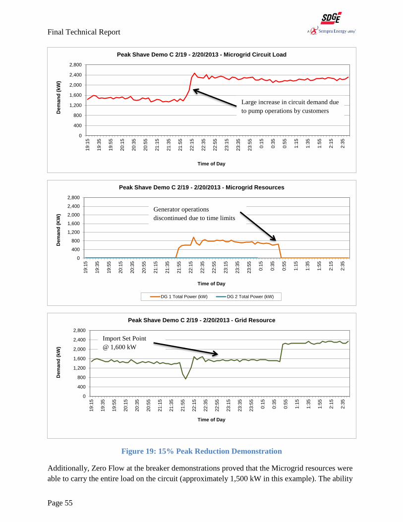
Final Technical Report
Page 55
Figure 19: 15% Peak Reduction Demonstration
Additionally, Zero Flow at the breaker demonstrations proved that the Microgrid resources were
able to carry the entire load on the circuit (approximately 1,500 kW in this example). The ability
0
400
800
1,200
1,600
2,000
2,400
2,800
19
:15
19
:35
19
:55
20
:15
20
:35
20
:55
21
:15
21
:35
21
:55
22
:15
22
:35
22
:55
23
:15
23
:35
23
:55
0:1
5
0:3
5
0:5
5
1:1
5
1:3
5
1:5
5
2:1
5
2:3
5
Dem
an
d (
kW
)
Time of Day
Peak Shave Demo C 2/19 - 2/20/2013 - Microgrid Circuit Load
0
400
800
1,200
1,600
2,000
2,400
2,800
19
:15
19
:35
19
:55
20
:15
20
:35
20
:55
21
:15
21
:35
21
:55
22
:15
22
:35
22
:55
23
:15
23
:35
23
:55
0:1
5
0:3
5
0:5
5
1:1
5
1:3
5
1:5
5
2:1
5
2:3
5
Dem
an
d (
KW
)
Time of Day
Peak Shave Demo C 2/19 - 2/20/2013 - Microgrid Resources
DG 1 Total Power (kW) DG 2 Total Power (kW)
0
400
800
1,200
1,600
2,000
2,400
2,800
19
:15
19
:35
19
:55
20
:15
20
:35
20
:55
21
:15
21
:35
21
:55
22
:15
22
:35
22
:55
23
:15
23
:35
23
:55
0:1
5
0:3
5
0:5
5
1:1
5
1:3
5
1:5
5
2:1
5
2:3
5
Dem
an
d (
kW
)
Time of Day
Peak Shave Demo C 2/19 - 2/20/2013 - Grid Resource
Large increase in circuit demand due
to pump operations by customers
Import Set Point
@ 1,600 kW
Generator operations
discontinued due to time limits

Final Technical Report
Page 56
to meet the 1,500 kW load on circuit using Microgrid resources represents a 100% reduction in
the actual load. Figure 20 on the following page shows the operation of one DG unit and the SES
carrying the entire load of the Microgrid Circuit. Prior to the demonstration, the circuit load was
a little more than 1,500 kW. The SES unit was operating in constant output at a rate of 250 kW.
The DG was operating in load following mode to a set point of 0 kW at Microgrid Circuit
Breaker. The combined operation of the DG and SES was able to carry the load on the circuit,
thereby managing the power at the Microgrid Circuit breaker to near zero.
The middle graph shows that the range of load fluctuation at the Microgrid Circuit Breaker was
-86 kW to + 43 kW. It is not clear if this fluctuation is due to the generator controls or the
accuracy of the transducer being used as the control point. The transducer is bi-directional with
a range of +/-8,000 kW. The variance of 129 kW represents an accuracy of 0.8%. This
demonstration showed the ability to control the load to near zero at the breaker in a manner that
the Microgrid should be able to transition to island mode while keeping the DG units operating
in a stable manner.

Final Technical Report
Page 57
Note: LF=Load Following; CO=Constant Output
Figure 20: Zero Flow at the Breaker Demonstration (Virtual Island)
0
20
40
60
80
100
9:2
0
9:4
0
10
:00
10
:20
10
:40
11
:00
11
:20
11
:40
12
:00
12
:20
12
:40
13
:00
Sta
te o
f C
harg
e (
%)
Time of Day
DG-LF & SES-CO Virtual Island Demonstration: 01/24/2013 - SES State of Charge
-300
0
300
600
900
1200
1500
1800
9:2
0
9:4
0
10
:00
10
:20
10
:40
11
:00
11
:20
11
:40
12
:00
12
:20
12
:40
13
:00
Dem
an
d (
kW
)
Time of Day
DG-LF & SES-CO Virtual Island Demonstration: 01/24/2013- Microgrid Resources
SES Output (kW) DG 1 Total Power (kW) DG 2 Total Power (kW)
-300
0
300
600
900
1200
1500
1800
9:2
0
9:4
0
10
:00
10
:20
10
:40
11
:00
11
:20
11
:40
12
:00
12
:20
12
:40
13
:00
Dem
an
d (
kW
)
Time of Day
DG-LF & SES-CO Virtual Island Demonstration: 01/24/2013- Grid Resource

Final Technical Report
Page 58
Objective 2: Demonstrate capability of Reactive power management
Results: Utilities use capacitors to compensate for reactive power caused by inductive loads.
Inductive loads involve equipment such as motors whose operation causes reactive power to
flow through the circuit. Capacitors provide reactive power compensation resulting in flatter
voltage profile along the circuit, and less energy wasted from electrical losses in the circuit. The
Borrego Springs Microgrid was designed with optimal reactive power management controls,
provided by the operation of Microgrid resources (DG and SES). Multiple demonstrations were
conducted using individual resources and a combination of resources to monitor the reactive
power on the circuit, and operate the resources to manage the reactive power flow at the
Microgrid Circuit Breaker. This section highlights two scenarios where the Microgrid resources
were operated to manage the reactive power flow on the circuit.
Figure 21 on the following page provides a summary of the demonstration which was conducted
on January 8, 2013. The Figure shows that during the first half of the operations the power
factor was adjusted to appropriate set points that lowered the reactive power on the Circuit.
Generator #2 was brought on line and operated in parallel with Generator #1 in order to have
enough VAr capacity to cancel the kVArs at the Microgrid Circuit Breaker.

Final Technical Report
Page 59
Figure 21: VAr Control Demonstration – Generators 1 and 2
Figure 22 on the following page provides a summary of the demonstration conducted on
November 26, 2012. The demonstration includes the operation of DG #1and DG #2 separately
and the SES unit operating during the entire demonstration. The DG units operated at a constant
output of 1,000 kW and power factor of .98 which contributed 180 kVAr. The kVAr setting on
the SES unit was set at various negative outputs (0, -200, and -400) for 15 minutes at each level
and then set at positive outputs (200, 400, and 0) during the operation of each generator. The
resultant reactive power as measured by the SCADA system was observed to move when the
changes in the Microgrid resource were adjusted in 200 kVAr increments. Thus, the
demonstrations showed that the reactive power as measured at the Microgrid Circuit Breaker by
the SCADA device could be controlled to specific levels with the DG units in combination with
the SES unit.
-50
0
50
100
150
200
10
:30
10
:50
11
:10
11
:30
11
:50
12
:10
12
:30
12
:50
13
:10
13
:30
kV
Ar
Time of Day
VAr Control Demo Setpoint A 01/08/2013 - Microgrid Circuit KVAr
0
50
100
150
200
10
:30
10
:50
11
:10
11
:30
11
:50
12
:10
12
:30
12
:50
13
:10
13
:30
kV
Ar
Time of Day
VAr Control Demo Setpoint A 01/08/2013- Microgrid Resources
DG 1 Reactive Power (KVAr) DG 2 Reactive Power (KVAr)
Circuit VArs
Near Zero
Adjust
Generator
Power Factor
Adjust
Generator
Power Factor
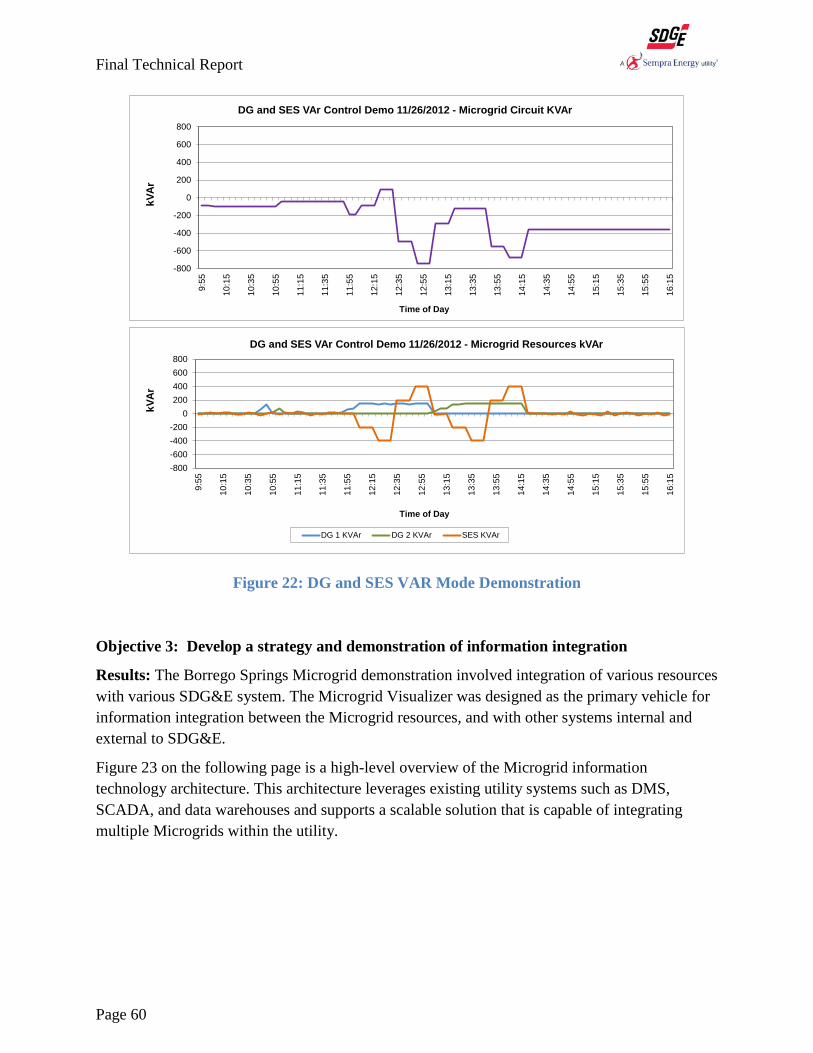
Final Technical Report
Page 60
Figure 22: DG and SES VAR Mode Demonstration
Objective 3: Develop a strategy and demonstration of information integration
Results: The Borrego Springs Microgrid demonstration involved integration of various resources
with various SDG&E system. The Microgrid Visualizer was designed as the primary vehicle for
information integration between the Microgrid resources, and with other systems internal and
external to SDG&E.
Figure 23 on the following page is a high-level overview of the Microgrid information
technology architecture. This architecture leverages existing utility systems such as DMS,
SCADA, and data warehouses and supports a scalable solution that is capable of integrating
multiple Microgrids within the utility.
-800
-600
-400
-200
0
200
400
600
800
9:5
5
10
:15
10
:35
10
:55
11
:15
11
:35
11
:55
12
:15
12
:35
12
:55
13
:15
13
:35
13
:55
14
:15
14
:35
14
:55
15
:15
15
:35
15
:55
16
:15
kV
Ar
Time of Day
DG and SES VAr Control Demo 11/26/2012 - Microgrid Circuit KVAr
-800
-600
-400
-200
0
200
400
600
800
9:5
5
10
:15
10
:35
10
:55
11
:15
11
:35
11
:55
12
:15
12
:35
12
:55
13
:15
13
:35
13
:55
14
:15
14
:35
14
:55
15
:15
15
:35
15
:55
16
:15
kV
Ar
Time of Day
DG and SES VAr Control Demo 11/26/2012 - Microgrid Resources kVAr
DG 1 KVAr DG 2 KVAr SES KVAr
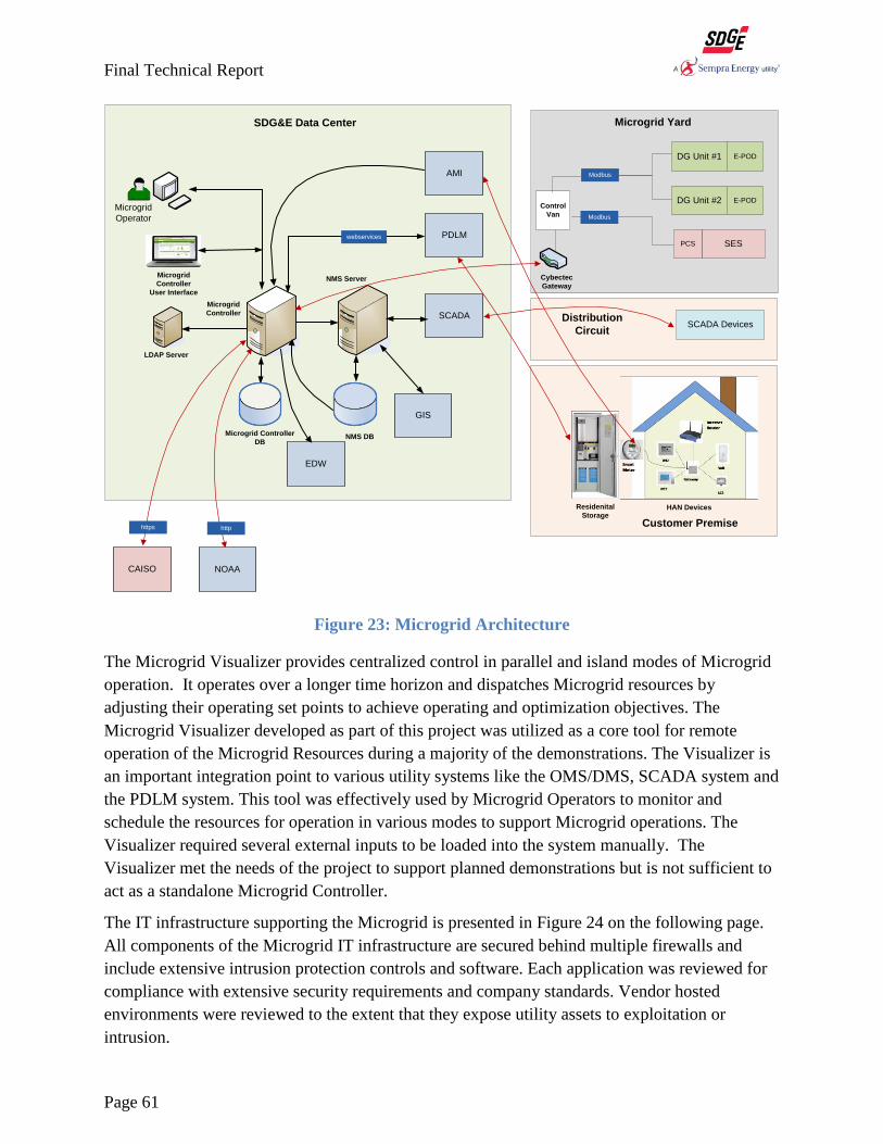
Final Technical Report
Page 61
Figure 23: Microgrid Architecture
The Microgrid Visualizer provides centralized control in parallel and island modes of Microgrid
operation. It operates over a longer time horizon and dispatches Microgrid resources by
adjusting their operating set points to achieve operating and optimization objectives. The
Microgrid Visualizer developed as part of this project was utilized as a core tool for remote
operation of the Microgrid Resources during a majority of the demonstrations. The Visualizer is
an important integration point to various utility systems like the OMS/DMS, SCADA system and
the PDLM system. This tool was effectively used by Microgrid Operators to monitor and
schedule the resources for operation in various modes to support Microgrid operations. The
Visualizer required several external inputs to be loaded into the system manually. The
Visualizer met the needs of the project to support planned demonstrations but is not sufficient to
act as a standalone Microgrid Controller.
The IT infrastructure supporting the Microgrid is presented in Figure 24 on the following page.
All components of the Microgrid IT infrastructure are secured behind multiple firewalls and
include extensive intrusion protection controls and software. Each application was reviewed for
compliance with extensive security requirements and company standards. Vendor hosted
environments were reviewed to the extent that they expose utility assets to exploitation or
intrusion.
SCADA
Microgrid
Operator
SDG&E Data Center
Microgrid Controller
DB
Microgrid
Controller
Microgrid
Controller
User Interface
NMS Server
NMS DB
PDLM
AMI
LDAP Server
GIS
CAISO
Control
Van
DG Unit #1 E-POD
DG Unit #2 E-POD
Modbus
SCADA Devices
SESPCS
Cybectec
Gateway
Microgrid Yard
Distribution
Circuit
https
webservices
EDW
Modbus
HAN DevicesResidenital
Storage
NOAA
httpCustomer Premise
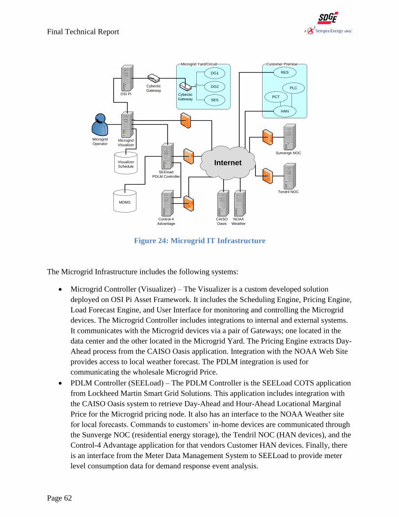
Final Technical Report
Page 62
Figure 24: Microgrid IT Infrastructure
The Microgrid Infrastructure includes the following systems:
Microgrid Controller (Visualizer) – The Visualizer is a custom developed solution
deployed on OSI Pi Asset Framework. It includes the Scheduling Engine, Pricing Engine,
Load Forecast Engine, and User Interface for monitoring and controlling the Microgrid
devices. The Microgrid Controller includes integrations to internal and external systems.
It communicates with the Microgrid devices via a pair of Gateways; one located in the
data center and the other located in the Microgrid Yard. The Pricing Engine extracts Day-
Ahead process from the CAISO Oasis application. Integration with the NOAA Web Site
provides access to local weather forecast. The PDLM integration is used for
communicating the wholesale Microgrid Price.
PDLM Controller (SEELoad) – The PDLM Controller is the SEELoad COTS application
from Lockheed Martin Smart Grid Solutions. This application includes integration with
the CAISO Oasis system to retrieve Day-Ahead and Hour-Ahead Locational Marginal
Price for the Microgrid pricing node. It also has an interface to the NOAA Weather site
for local forecasts. Commands to customers’ in-home devices are communicated through
the Sunverge NOC (residential energy storage), the Tendril NOC (HAN devices), and the
Control-4 Advantage application for that vendors Customer HAN devices. Finally, there
is an interface from the Meter Data Management System to SEELoad to provide meter
level consumption data for demand response event analysis.
Visualizer
Schedule
Microgrid
Visualizer
Microgrid Yard/Circuit
DG1
DG2
SES
OSI Pi
SEEload
PDLM Controller
Customer Premise
RES
PLC
PCT
HAN
Tendril NOC
Control-4
Advantage
CAISO
Oasis
NOAA
Weather
Internet
Sunverge NOC
Microgrid
Operator
Cybectic
Gateway
Cybectic
Gateway
MDMS

Final Technical Report
Page 63
Network Operation Center (Tendril) – The PDLM Controller communicates all device
commands to the HAN vendors NOC. The HAN vendors are responsible for the
infrastructure, management and communication to the individual customer’s HAN
controller and devices. The NOC also provides customer device status information back
to the PDLM controller.
Network Operations Center (Sunverge) – The PDLM controller communicates
commands for the residential energy storage through the vendor’s (Sunverge) network
operation center. As with the Tendril NOC, the Sunverge NOC manages all
communication to the installed customer RES. Sunverge also provides PDLM with
device status.
Objective 4: Develop a strategy and demonstrate the integration of Advanced Meter
Infrastructure (AMI) into Microgrid operations
Results: The Borrego Springs Microgrid integrated with the Advanced Metering Infrastructure
to provide interval meter data from the Smart Meter for Demand Response forecasting. The
meter data was also used for Measurement and Verification of event data after Demand
Response events were executed. This information helped analyze the actual load reduction
versus predicted load reduction. This section describes the demand response forecast and post
event analysis processes that utilized the meter data from the AMI system.
Demand Response Forecast - The primary objective of these demonstrations was to gather
sufficient data to develop Demand Response forecasts with the required confidence levels within
the PDLM Controller. The PDLM Controller develops a DR capacity forecast on a rolling 48-
hour basis. The forecast is a learning algorithm that improves and converges over time. The
baseline data initially utilized by the PDLM Controller vendor to develop the load forecast was
based on typical Customer Baseline Load (CBL). The CBL data was developed by analyzing
historical meter interval data, extracted from the AMI system. The forecast algorithm utilized the
CBL to forecast DR Capacity on the Microgrid Circuit. The initial DR forecast did not converge
for the expected Demand Response on the Microgrid Circuit. The PDLM Controller allowed for
applying a correction factor that would reduce the CBL ratio, thereby reducing the DR Capacity
Forecast. This resulted in the initial DR Capacity forecast that did not represent the true nature of
DR on the Microgrid Circuit. The Microgrid team applied correction factors that provided a
reasonable DR Capacity Forecast for the Microgrid Circuit. Figure 25 on the following page
presents the initial DR Capacity forecast.

Final Technical Report
Page 64
Figure 25: Initial DR Capacity Forecast
Figure 26 presents the DR Capacity Forecast provided by the PDLM Controller after application
of correction factors to CBL.
Figure 26: DR Capacity Forecast – After Correction Applied to CBL
Post Event Analysis- Once a Demand Response event was completed successfully, the PDLM
system conducts a post event Measurement and Verification analysis and results. This provides a

Final Technical Report
Page 65
feedback loop to refine the DR capacity estimates for future events. It also allows the operator to
develop a confidence level for specific programs so that more accurate DR capacity estimates are
possible.
The M&V process uses meter data from the AMI system to assess the actual load reduction from
the DR event. This is necessary because not all HAN devices are aware of the load they carry. In
some cases, the devices can record the actual load. For example, the plug load controller where
the current flows through the device is able to capture the load data. This is reported to the
device vendor NOC through the HAN Gateway. In the case of the PCT, however, the load
measurable at the thermostat is not the same as the load of the compressor. Therefore, these
devices cannot report any actual load. Most of the load reduction in a typical DR event comes
from PCTs. The load of a central air conditioning system is significantly greater than that of a
plug load controller for a lamp. Therefore, the actual load reduction can only be measured
indirectly. One can only infer that the reduction was a result of the DR event.
The PDLM system calculates the actual load reduction by comparing the forecasted load to the
actual load. Any difference is attributed to the devices participating in the DR event. The
difference is considered the “actual load reduction.” The actual load reduction is then compared
to the forecasted load reduction. Any difference in these values is used to adjust the expected
load reduction for each device in future DR capacity estimates. The operator has the choice to
accept and apply or reject the adjustments for future DR capacity estimates
The PDLM’s Analysis Module displays a table of completed events with the following summary
data for each event:
Event Date
Event Start Time
Event End Time
Duration
Predicted load reduction
Actual load reduction
Percent Participation
Percent Opt Out
The predicted load reduction is forecast based specific programs. Each program has an
“Estimated DR Capacity” based on:
Starting assumptions for the device type (Customer Baseline Load)
Historical actual results from DR events and analysis
Temperature forecast (in the case of PCT)
The actual load reduction uses hourly interval Meter Data from which the PDLM records the
consumption for the entire customer premises which is the difference between the CBL and the
Actual Load on the customer premises. Customers were provided with incentives to participate

Final Technical Report
Page 66
in all DR and RTP demonstrations. However they had the option to opt out of events, if
necessary. Percent Participation captures the percentage of customers that participated in the
demonstration, while Percent Opt Out captures the percentage of customers that opted out of the
demonstration.
Since the post event data represents the load impact of the aggregated customer base, further
analysis was performed to understand the effect of DR events on individual customer load
reduction. Hourly customer interval data was obtained from the AMI system for customers that
participated in the DR demonstrations. The data was analyzed to see the trend of customer load
on the days of the event and an average of the customer load over 3-days or 7-days prior to the
event. This analysis identified several instances of actual load reduction in customer homes
during the DR demonstrations. In absence of the DR events, the customer load would have
remained higher. Figure 27 presents the load profile for certain customers who participated in the
DR events who had significant load reduction of during the DR events. The charts below present
two load curves for comparison:
Event Day Load Curve ( red line)
Average Load for Days Prior to Event (black line)
Figure 27 presents the results of a three hour DR event that was executed between 14:00
and 17:00. The customer had a slight reduction in load during the first and second hours
of the event and then a more substantial reduction in the third hour of the event. Overall,
the customer load was higher than their average load when the event began and was
lower than their average load at the end of the event. The load reduction from the
beginning of the event to the end of the event was 6.6 kW
Figure 27: Example - Customer Load Reduction During DR Events
0.0
2.0
4.0
6.0
8.0
10.0
12.0
1:0
0
2:0
0
3:0
0
4:0
0
5:0
0
6:0
0
7:0
0
8:0
0
9:0
0
10
:00
11
:00
12
:00
13
:00
14
:00
15
:00
16
:00
17
:00
18
:00
19
:00
20
:00
21
:00
22
:00
23
:00
0:0
0
De
ma
nd
(kW
)
Time of Day
AMI Data
Event Day Average Load for Days Prior to Event
DR EventDR Event
DR Event

Final Technical Report
Page 67
Objective 5: Develop a strategy and demonstrate ‘self-healing’ networks
Results: The FLISR was first modeled for the Microgrid Circuit and was tested in a
development platform and then moved into production. For a detailed assessment of the
improvement in response to unplanned outage, the switch plans were analyzed for all outages on
the Microgrid Circuit. The outages were analyzed to identify those that were representative of
events that could be impacted by FLISR. This eliminated outages that could not be switched
using available SCADA devices. Nine representative outages were identified and analyzed, to
assess the expected benefit on the results of simulation compared to actual historic outage
operations results.
1. Momentary Outage of Less than 1 Minute Caused by Weather
2. Sustain Outage Caused by Motor Vehicle Collision
3. Sustained Outage Caused by Damaged Pole
4. Sustained Outage Caused by Tree Overhead Wire Down
5. Sustained Outage Caused by Equipment Failure and Overhead Wire Down
6. Sustained Outage Caused by Overhead Wire Down
7. Sustained Outage Caused by Overhead Equipment Failure
8. Sustained Outage Resolved by Auto-Sectionalizer
9. Sustained Outage Caused by Earthquake
Based on demonstrations and performance metrics observed in the Microgrid Circuit, FLISR has
the opportunity to improve Customer experience and circuit reliability through:
Reduced customer duration minutes
Reduced number of customers included in sustained outages
Improve distribution operators efficiency
The FLISR system impact on historic outages described above includes:
Three events that would not have changed
One momentary event that would have been completed two minutes faster
Four sustained events that would have had a subset of customers converted from a
sustained to a momentary outage and reduced duration significantly
One sustained outage that would have been converted to a 2 minute momentary outage
provided that earthquake policy could accommodate FLISR operation
Improving the efficiency of distributions operators is one of the significant contributions of
FLISR. It is difficult to quantify these efficiency benefits. Operators are responsible for multiple
tasks. They schedule time throughout the day to manage the distribution network for planned
work by the construction crews. Distribution operations must be staffed to support ongoing
planned activity. They must also have the capacity to respond to unplanned events such as
outages.
FLISR improved efficiency in several ways. The essence of the improvement is that the
distribution operators are presented with a simpler contained outage. Rather than dealing with the

Final Technical Report
Page 68
entire circuit, the operators only deal with the isolated faulted segment of the circuit. Also, the
operator does not have to deal with the switch planning and execution for isolation and
restoration. This allows the operator to focus efforts on the high value efforts to direct and
support the assigned troubleshooting and repair crews.
Benefits of reducing and simplifying the process extends to unrelated tasks assigned to the
distribution operators. Interruptions to ongoing planning and workflows are fewer and shorter.
This allows the operators to return to planned activities more quickly. Their productivity when
returning to these tasks is higher when the interruptions are shorter and simpler.
Objective 6: Develop a strategy and demonstrate the integration of an OMS/DMS into
Microgrid operations
Results: The Microgrid Visualizer developed as part of this project was utilized as a core tool
for remote operation of the Microgrid Resources during a majority of the demonstrations. The
Visualizer is an important integration point to various utility systems like the OMS/DMS,
SCADA system and the PDLM system. This tool was effectively used by Microgrid Operators to
monitor and schedule the resources for operation in various modes to support Microgrid
operations. The Visualizer required several external inputs to be input into the system manually.
The Visualizer met the needs of the project to support planned demonstrations but is not
sufficient to act as a standalone Microgrid Controller.
Figure 28 presents a high level view of the various systems integrated together to integrate with
the Microgrid Visualizer.
Figure 28: Interaction between Distribution System Operations and Microgrid Operations
OMS/DMS
FLISR
SCADA
Microgrid
Visualizer
Microgrid
Circuit
Resources
PDLM
NOAA
CAISO
Load Forecast
CAISO Price
DR Event Trigger
Schedule Resources
Schedule DR Resources
Wholesale Price
Weather
Distribution
System
Operator
Microgrid
Operator
Substation

Final Technical Report
Page 69
The Distribution System Operator (DSO) oversees the operational functions of the entire
distribution network through a newly implemented OMS/DMS system that is also is interfaced to
SCADA system. The OMS/DMS system supports distribution system operations and also
includes tools for Volt/VAr management, validation of switching plans as well as FLISR
activities.
The Microgrid Visualizer was developed as the system of record to monitor and schedule
operations of the Distributed Energy Resources within the Microgrid. The Microgrid Visualizer
was created based on an iterative process that began by developing business and technical
functional requirements for a Microgrid controller. As part of the Microgrid demonstration, the
PDLM system was developed to manage customer-owned resources for DR. The Microgrid
Visualizer interfaces with the PDLM system, and provides triggers to the PDLM system which
can schedule and dispatch DR resources as needed.
The Microgrid Operator is the point of contact to oversee and manage the control and monitoring
functions for the Microgrid. The Microgrid Operator manages the Visualizer and the PDLM
system. The Microgrid Operator is also responsible for translating the data from CAISO
(Wholesale Price to retail price conversion) and NOAA (weather data) to actions that affect
Microgrid system operations. The major activities of the Microgrid operator include:
Develop a daily load forecast and input into Microgrid Visualizer
Collect the appropriate day ahead CAISO Wholesale Price and input into the Microgrid
pricing model
Schedule Microgrid Resources to optimize Microgrid operations
Create DR Event Trigger within the PDLM System as needed
Schedule DR Resources within the PDLM System
Objective 7: Demonstrate the capability to use automated distribution control to
intentionally island customers in response to system problems.
Results: The Borrego Springs Microgrid was designed to operate the Microgrid in island mode.
Multiple demonstrations were performed that proved the Microgrid can seamlessly transition
into island operation and seamlessly transition back to parallel mode of operation. This section
provides information on the demonstrations that were conducted island the Microgrid with real
customers.
The key objectives of the island demonstrations are as follows:
Operate the Microgrid Resources to a condition of zero power flow at the breaker and
open the Microgrid Circuit Breaker while maintaining stability of the Microgrid Circuit
Validate the isochronous operation of the DG units
Validate stable operation of the islanded Microgrid Circuit while operating the DG and
SES units together

Final Technical Report
Page 70
Quantify the level of reactive power support that the SES can provide to the DG units
while in island operations
Validate the seamless transition of the Microgrid from island mode back to the grid
Overall there were seven Island demonstrations that were conducted as presented in Table 9. For
the first two Island demonstrations, three separate sub-demonstrations were conducted that
included:
Island with Distributed Generators Only
Island with Distributed Generators and Substation Energy Storage together
Island with Distributed Generators and Substation Energy Storage for VAr Control
Table 9: Island Operation Demonstrations
Island with Distributed Generators Only - Island Operation with DG only was conducted as
the first Island demonstration because the generators had been modified with controls to
specifically operate in an isochronous mode of operation. Also, the demonstrations were
conducted at a time when the load on the Microgrid Circuit could be carried by the two 1.8 MW
generator units. The specific objectives of this demonstration included:
Demonstrate Generator operation in Isochronous mode for
o Load Control
o Voltage Control
o VAr Control
o Frequency Control
Demonstrate Stability of Operation of the Microgrid Circuit while in Island
Demonstrate Seamless Transitions of the Microgrid Circuit for the following:
o Generator synchronization to the grid
o Separation of Microgrid from the grid
o Return of Microgrid back to the grid
The Sequence of Operation to operate Microgrid Circuit in Island mode with DG only included:
Switch off the line capacitor on the Microgrid Circuit
Synchronize generators to match grid voltage and frequency
Mode of
OperationDemo Description Control Settings Demo Date
Start
Time
End
Time
Control
Interface
Gen1 Gen 2 SES
X X Island Demonstration w/DG Only Gen 1 and Gen 2 2/13/2013 9:20 10:35 Local
X X X Island Demonstration w/DG and SES Gen 1, Gen 2 and SES (Real Power) 2/13/2013 10:45 11:40 Local
X X X Island Demonstration w/DG and SES VArGen 1, Gen 2 and SES (Real Power and
Reactive Power)2/13/2013 11:50 12:40 Local
X X Island Demonstration w/DG Only Gen 1 and Gen 2 2/27/2013 9:00 10:15 Local
X X X Island Demonstration w/DG and SES Gen 1, Gen 2 and SES (Real Power) 2/27/2013 9:00 10:10 Local
X X X Island Demonstration w/DG and SES VArGen 1, Gen 2 and SES (Real Power and
Reactive Power)2/27/2013 10:15 11:45 Local
X X X Remote Island DemonstrationGen 1, Gen 2 and SES (Real Power and
Reactive Power)3/13/2013 10:00 14:20 Remote
Microgrid Resources
Island
Test

Final Technical Report
Page 71
Set the generators in load following mode with set point of zero (zero power flow across
the Microgrid Circuit Breaker)
Once the power flow across the Microgrid Circuit Breaker is zero, request island
permissive bit.
Microgrid Circuit Breaker opens
Observe the generator controls to automatically transition to the isochronous mode
Operate in Island Mode for approximately one hour
Once the Island operation is successfully operational for one hour, synchronize back to
Grid (upstream of Microgrid Circuit Breaker)
Microgrid Circuit Breaker closes
Leave Generators running in parallel for next demonstration
The above sequence of operations was a result of close cooperation between the Microgrid
Operator and the Distribution System Operators.
The Island Operations using only the generators was demonstrated successfully by locally
controlling the generators using the Microgrid Visualizer. The first two times that the island
mode was demonstrated, the Microgrid Operator controlled the equipment from the Control Van
in the Microgrid Yard. The operations were coordinated with a line crew to manually turn off
the fixed line capacitor at the beginning of the demonstration and to be available for other
support if needed.
Figure 29 on the following page presents a summary of the island demonstration on February 13,
2013. For this demonstration, DG #1 was initially synchronized with the Microgrid Circuit with
a load of approximately 1,600 kW. Then DG #2 was synchronized with the Microgrid Circuit
and the load was shared equally by both generators. The two units operated in load following
with a set point of 0 kW at the Microgrid Circuit Breaker from 9:27 AM to 9:40 AM when the
Distribution Operator sent a permissive bit to island the Microgrid Circuit. The Microgrid
operated as an island for 90 minutes. The Distribution System Operator set the permission in the
relay for the generators to synchronize back to the grid. The synchronization took approximately
45 seconds, (the controls are configured for 2-minute time-out). Once the Microgrid Circuit
Breaker was closed, the two generators operated again in load following with a set point of 0 kW
and remained in this mode until 10:37 AM.

Final Technical Report
Page 72
Figure 29: Island Demonstration with DG Only
Figure 30 shows the DG #1 controls while operating in an island demonstration. The unit is
operating at 970 kW, 479 volts, a power factor of 0.98 lagging, and a frequency of 60.02 Hz.
0
400
800
1,200
1,600
2,000
9:0
0
9:0
4
9:0
8
9:1
2
9:1
6
9:2
0
9:2
4
9:2
8
9:3
2
9:3
6
9:4
0
9:4
4
9:4
8
9:5
2
9:5
6
10
:00
10
:04
10
:08
10
:12
10
:16
10
:20
10
:24
10
:28
10
:32
10
:36
10
:40
10
:44
10
:48
10
:52
10
:56
De
ma
nd
(kW
)
Time of Day
Microgrid Circuit Load 02/13/2013 - Island Test w/DG only
0
400
800
1,200
1,600
2,000
9:0
0
9:0
4
9:0
8
9:1
2
9:1
6
9:2
0
9:2
4
9:2
8
9:3
2
9:3
6
9:4
0
9:4
4
9:4
8
9:5
2
9:5
6
10
:00
10
:04
10
:08
10
:12
10
:16
10
:20
10
:24
10
:28
10
:32
10
:36
10
:40
10
:44
10
:48
10
:52
10
:56
Dem
an
d (
KW
)
Time of Day
Microgrid Resources 02/13/2013 - Island Test w/DG only
DG 1 Total Power (kW) DG 2 Total Power (kW)
0
400
800
1,200
1,600
2,000
9:0
0
9:0
4
9:0
8
9:1
2
9:1
6
9:2
0
9:2
4
9:2
8
9:3
2
9:3
6
9:4
0
9:4
4
9:4
8
9:5
2
9:5
6
10
:00
10
:04
10
:08
10
:12
10
:16
10
:20
10
:24
10
:28
10
:32
10
:36
10
:40
10
:44
10
:48
10
:52
10
:56
Dem
an
d (
kW
)
Time of Day
Grid Resource 02/13/2013 - Island Test w/DG only
Island Operation

Final Technical Report
Page 73
Figure 30: Generator Control Display in Island Operations
Figure 31 presents the generator synchroscope during the transition from island to grid
connected. The synchronization process took less than 45 seconds to complete. The breaker
closes when the synchronization indicator is stable at the 12 o’clock position on the circle.
Figure 31: Generator Synchroscope during Transition from Island
Additional monitoring was conducted during the island demonstrations to evaluate the voltage on
the 12 kV Microgrid Circuit during the various transition points. Figure 32 on the following
page shows the voltages on the three circuit phases as the DG units synchronize to the grid and
when the Microgrid Circuit Breaker opens. The data shows that there is a perturbation of
voltages at each transition with the largest occurring when the circuit breaker opens. The
Microgrid Circuit
Breaker in Open
Position
Synchronization
Indicator

Final Technical Report
Page 74
fluctuation of voltage when the circuit breaker opens is about 70 volts with represents a 0.6%
voltage fluctuation.
Figure 32: Microgrid Circuit Voltage when Transitioning into Island
Figure 33 on the following page shows the voltages on the three phases of the circuit when the
Microgrid Circuit Breaker closes. The data shows that there is a perturbation of voltages at the
transition. Both figures show that the voltages are slightly higher when the generators are
operating in the island. At all times, the voltages are within the standards of delivery to the
customers.
DG #1 Synchronizes to Grid
DG #2 Synchronizes to Grid
Circuit Breaker Opens

Final Technical Report
Page 75
Figure 33: Microgrid Circuit Voltage when Transitioning from Island
Island with Distributed Generation and SES - With the successful Island Demonstration of
the Microgrid Circuit with DG only, the next objective was to demonstrate Island Operation with
simultaneous operation of the DG and SES units. Additional objectives of this demonstration
include:
Demonstrate Stability of Operation of the Microgrid Circuit while in Island
Demonstrate ability to vary SES discharge rates in Island mode
Demonstrate ability to transition the SES to charge mode in Island operation
Demonstrate ability to vary charge rates in Island mode
Demonstrate Seamless Transitions of the Microgrid Circuit for the following:
o Generator synchronization to the grid
o Separation of microgrid from the grid
o Return of Microgrid back to the grid
Methodology – The Sequence of Operation to operate Microgrid Circuit in Island mode with
DG and SES included:
Parallel SES with the Microgrid Circuit in discharge mode
Parallel DG units with the Microgrid Circuit in load follow with set point of zero (zero
power flow across the Microgrid Circuit Breaker)
Once the power flow across the Microgrid Circuit Breaker is zero, request island
permissive bit.
Microgrid Circuit Breaker opens
Operate in Island Mode with DG and SES for approximately one hour
Grid Connected Operation
Circuit Breaker Closes
Island Operation

Final Technical Report
Page 76
SES Operation while in Island Mode:
o Discharge SES at 100 kW for 15 minutes
o Ramp SES down to 0 kW in 10 kW steps over a one minute period
o Operate SES at 0 kW for 15 minutes
o Ramp SES down to -100 kW (charge mode) in 10 kW steps over a one minute
period
o Charge SES at 100 kW for 15 minutes
o Ramp SES up to 100 kW in 10 kW steps over a two minute period
o Discharge SES at 100 kW for 15 minutes
Once the Island operation is successfully operational for one hour, synchronize back to
Grid (upstream of Microgrid Circuit Breaker)
Microgrid Circuit Breaker closes
Leave Generators running in parallel for next demonstration
The Island Operations with DG and SES only was demonstrated successfully by controlling the
generator and SES locally using the Microgrid Visualizer from the Control Van in the Microgrid
yard. The control approach demonstrated that the DG and SES can be operated simultaneously
to meet a forecasted load. The DG was operated in load following and while the SES was
programmed to operate within specified set points. Figure 35 on the following page shows that
the generators and SES were able to share and meet the load over the range of operation.
The SES was operated in both charge and discharge modes of operation and the set points were
also altered during the demonstration. The point of adjusting the SES set points was to cause
small rapid changes in the load seen by the DG units and observe if the stability of the island
mode operation was affected by these changes. Figure 34 presents a screen shot of the Microgrid
Visualizer during island operation with both DG units and the SES operating.
Figure 34: Microgrid Visualizer during Island Operations
Microgrid Operating in Island Mode:• Microgrid Circuit Breaker Open• Island Operation Permission Granted• Microgrid Resources:
• SES: 100 kW• Gen#1: 677 kW / 99 kVAr• Gen #2: 656 kW / 277 kVAr
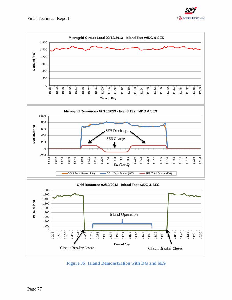
Final Technical Report
Page 77
Figure 35: Island Demonstration with DG and SES
0
300
600
900
1,200
1,500
1,800
10
:28
10
:32
10
:36
10
:40
10
:44
10
:48
10
:52
10
:56
11
:00
11
:04
11
:08
11
:12
11
:16
11
:20
11
:24
11
:28
11
:32
11
:36
11
:40
11
:44
11
:48
11
:52
11
:56
12
:00
Dem
an
d (
kW
)
Time of Day
Microgrid Circuit Load 02/13/2013 - Island Test w/DG & SES
-200
0
200
400
600
800
1,000
10
:28
10
:32
10
:36
10
:40
10
:44
10
:48
10
:52
10
:56
11
:00
11
:04
11
:08
11
:12
11
:16
11
:20
11
:24
11
:28
11
:32
11
:36
11
:40
11
:44
11
:48
11
:52
11
:56
12
:00
Dem
an
d (
KW
)
Time of Day
Microgrid Resources 02/13/2013 - Island Test w/DG & SES
DG 1 Total Power (kW) DG 2 Total Power (kW) SES Total Output (kW)
0
200
400
600
800
1,000
1,200
1,400
1,600
1,800
10
:28
10
:32
10
:36
10
:40
10
:44
10
:48
10
:52
10
:56
11
:00
11
:04
11
:08
11
:12
11
:16
11
:20
11
:24
11
:28
11
:32
11
:36
11
:40
11
:44
11
:48
11
:52
11
:56
12
:00
Dem
an
d (
kW
)
Time of Day
Grid Resource 02/13/2013 - Island Test w/DG & SES
SES Discharge
SES Charge
Circuit Breaker Opens Circuit Breaker Closes
Island Operation

Final Technical Report
Page 78
Island with Distributed Generation and SES (VAr Control) - The primary objective of this
particular islanding demonstration is to evaluate how the Microgrid resources can effectively
manage reactive power in island operation. This demonstration builds on the simultaneous
operation of DG and SES in Island mode to evaluate options for VAr control during Island
operation. In isochronous operation, the DG units supply the reactive power required by the
circuit loads which can be high when the large pumps are operating. The goal of this scenario is
to evaluate the ability to have the DG units provide a majority of the real power to the Microgrid
and to have the SES unit provide a majority of the reactive power. This method of operation is
expected to result in a lower cost of operation and provide the ability to potentially operate the
generators longer since they will be consuming less fuel by operating more efficiently.
Additional objectives of this demonstration include:
Demonstrate Stability of Operation of the Microgrid Circuit while in Island
Demonstrate ability to conduct SES operations (on/off) in Island mode
Demonstrate ability to control VArs in Island mode
The Sequence of Operation to operate Microgrid Circuit in Island mode with DG and SES
managing the VAr on the circuit included:
Parallel SES with the Microgrid Circuit in idle mode
Parallel DG units with the Microgrid Circuit in load follow with set point of zero (zero
power flow across the substation breaker)
Once the power flow across the substation breaker is zero, request island permissive bit
Microgrid Circuit Breaker opens
Operate in Island Mode with DG and SES for approximately 45 minutes
Set SES in Base Mode
Ramp SES to 100 kW
Place the SES in VAr control mode and adjust VAr output to minimize VArs on the
circuit
Once the Island operation is successfully operational for 45 minutes, operate the SES in
idle mode
Synchronize back to Grid with generator controls at the Microgrid Circuit Breaker
Microgrid Circuit Breaker closes
The Island Operation with DG and SES controlling VArs was demonstrated successfully by
locally controlling the generator and SES from the Control Van in the Microgrid yard using the
Microgrid Visualizer. The two DGs operated in isochronous mode and the SES operated in VAr
mode to provide the required VArs on the circuit. The SES was not able to carry the full VAr
load on the circuit; however, the use of SES for VAr control meant that the generators could be
operated at a higher power factor of 0.95, thereby carrying more load on the circuit. The SES
was initially operated in idle mode, then ramped up to discharge at 100 kW and was finally
placed back in idle mode. This demonstrated the capability to operate the SES in Island mode

Final Technical Report
Page 79
without affecting the stability of the Microgrid Circuit. Finally, the Microgrid Circuit seamlessly
transitioned from Island operation to grid parallel operation within 45 seconds.
Figure 36 shows that the generators are operating by themselves at a power factor approximately
0.90. At 12:00 PM the SES reactive power output was set to 100 kVAr, which allowed the
generators to operate at a power factor of approximately 0.92. At 12:10 PM the SES reactive
power output was increased to 275 kVAr, which improved the generator power factor to 0.95.
This demonstrated that the SES could manage VAr to the point where the generators could
operate at improved power factors. The duration of the demonstration was from 11:40 AM to
12:45 AM. The Microgrid Circuit load ranged between 1,650 kW and 1,400 kW during the
demonstration.
Figure 36: Island Demonstration with DG using SES for VAr Control
Objective 8: Develop information/tools addressing the impact of multiple DER
technologies.
Results: The Microgrid was designed to operate multiple DER technologies that integrated with
the Microgrid Visualizer. Various information tools and processes were developed that assisted
in Microgrid operations.
Microgrid Visualizer –The Microgrid Visualizer interfaces with the various resources on the
Microgrid Circuit, as well as various systems at SDG&E. Each individual resource in the
Microgrid Circuit is equipped with its internal control system. Various systems at SDG&E like
SCADA, OMS/DMS, and PDLM system have their own user interfaces that provide into the
control functions that are available to the operator. With so many user interfaces to monitor, it
would have been difficult for the Microgrid Operator to get an overall picture of the information
flow across these systems.
The Microgrid Visualizer provides a consolidated user interface for the Microgrid Operator to
dispatch resources and monitor equipment operation. When a desired set of operations are
-50
0
50
100
150
200
250
300
800
850
900
950
1,000
11
:30
11
:34
11
:38
11
:42
11
:46
11
:50
11
:54
11
:58
12
:02
12
:06
12
:10
12
:14
12
:18
12
:22
12
:26
12
:30
12
:34
12
:38
12
:42
12
:46
12
:50
kV
Ar
Po
we
r F
ac
tor
X 1
00
0
Time of Day
Microgrid Resources kVAr 02/13/2013- Island Test w/DG & SES VAr
DG Power Factor SES KVAr
DG Warm up –
Not Grid
Connected
DG Only
SES Increases VAr Output
and DG PF increases
DG Operating
at .95 PF

Final Technical Report
Page 80
needed for the Microgrid, the Microgrid Operator selects, loads, and activates the appropriate
schedule or profile. Figure 37 presents the Microgrid Visualizer user interface when a scheduled
operation is being executed. This interface provides the Microgrid Operator with the status and
operating parameters of each of the Microgrid Resources as well as the scheduled operation.
This provides feedback to the Operator whether or not the Microgrid is operating as anticipated.
Figure 37: Microgrid Visualizer User Interface
Load Forecast - A load forecast model was developed using August 2012 data to help support
Microgrid operations and demonstration planning. The load forecast is based on a multivariable
linear regression using the following variables:
Time of day (military format with no colon)
Outside ambient dry bulb air temperature forecast (oF)
Pump schedule flag ( 1’s and 0’s, set to 1 from 11:00 PM to 5:00 AM)
Average of three previous weekday’s load at the same time day (MW)
Average of three previous weekday’s ambient dry bulb Air temperatures at the same time
(oF)
Figure 38 presents a sample load forecast versus actual load that was observed for 2/6/2013.

Final Technical Report
Page 81
Figure 38: Example Load Forecast
Microgrid Pricing - The Pricing Module is used to calculate the wholesale price of electricity
($/MWh) for electricity delivered to customers within the Microgrid. The wholesale price is
dependent on the operation of Microgrid Resources in along with the transmission grid. If the
Microgrid resources are non-operational, the wholesale price is equal to the Locational Marginal
Price at the Borrego node. This LMP nodal price is obtained through an interface with CAISO’s
Nodal LMP system (referred to OASIS). If the Microgrid resources are operational, the
wholesale price is calculated by calculating an average weighted price of energy obtained from
the grid at the LMP nodal price and the price of energy produced by the operating Microgrid
Resources.
The wholesale price consists of the following components:
DG #1 Price – Price associated with the operation of Distributed Generator #1
DG #2 Price – Price associated with the operation of Distributed Generator #2
Grid Price - The Grid Price is equal to the CAISO DAM LMP price for the Borrego Node
SES Price – Price associated with the charge/discharge operation of the Substation
Energy Storage unit
CAISO wholesale prices were downloaded from the CAISO OASIS website on a daily basis.
The data was available in a comma separated values file and was transferred to the Microgrid
Visualizer. An internal script running on the Microgrid Visualizer picked up the CAISO price
and transferred the values to the Pricing Module once every 24-hours.
The base formula to calculate the Total Weighted Average Price (𝑀𝑖𝑐𝑟𝑜𝑔𝑟𝑖𝑑 𝑃𝑟𝑖𝑐𝑒$/𝑀𝑊ℎ) is:
(𝑀𝑊𝐷𝐺1 ∗ $
𝑀𝑊𝐻𝐷𝐺1) + (𝑀𝑊𝐷𝐺2 ∗
$
𝑀𝑊𝐻𝐷𝐺2) + (𝑀𝑊𝑆𝐸𝑆 ∗
$
𝑀𝑊𝐻𝑆𝐸𝑆) + (𝑀𝑊𝐺𝑅𝐼𝐷 ∗
$
𝑀𝑊𝐻𝐺𝑅𝐼𝐷)
𝑀𝑊𝐷𝐺1 + 𝑀𝑊𝐷𝐺2 + 𝑀𝑊𝑆𝐸𝑆 + 𝑀𝑊𝐺𝑅𝐼𝐷
An exception to this calculation occurs when the SES is in the charging mode. The Total
Weighted Average Price (𝑀𝑖𝑐𝑟𝑜𝑔𝑟𝑖𝑑 𝑃𝑟𝑖𝑐𝑒$/𝑀𝑊ℎ) during the charging interval is calculated by

Final Technical Report
Page 82
excluding the SES Aggregate Price component. The value of electricity in the SES unit is
accounted for by using the LMP price at the time of the charging and the quantity of electricity
added to the SES while charging. Prior to discharging the SES unit, the average cost of
electricity for all the energy stored in the unit is calculated. This is used as the basis of the price
of energy from the SES unit during the entire discharge cycle.
Table 10 presents the total weighted average price calculation for a simulation of Microgrid
resources running on January 15, 2013. DG# 1 and DG# 2 were operating for two hours between
11:00 AM to 1:00 PM, while the SES was discharging between 10:00 AM to 12:00 noon. The
CAISO wholesale price for that particular day is shown in the third column. The Table shows
that at time periods when the DG unit or the SES is not operating, the Microgrid price is equal to
the CAISO Price. During time periods when the DG units and SES were operated the Microgrid
price is calculated and the associated Microgrid Price is calculated.
Table 10: Microgrid Price Calculation – 01/15/2013 Simulation
An example wholesale price as posted on the CAISO website for 01/15/2013 is presented in
Figure 39 on the following page.
CAISO Price Microgrid Price
Date Time
LMP
($/M
Wh)
Fuel
Flo
w
(Gal
lons
/Min
)
Gal
lons
/Hou
r
kW
Hou
rly
Cos
t
$/M
Wh
Fuel
Flo
w
(Gal
lons
/Min
)
Gal
lons
/Hou
r
kW
Hou
rly
Cos
t
$/M
Wh
kW (
ES C
harg
e
Rat
e)
Incr
emen
tal
Dol
lars
$ B
alan
ce
SOC
Ava
ilabl
e
Cap
acit
y M
Wh
$ B
alan
ce
$/M
Wh
kW
Hou
rly
Cos
t
$/M
Wh
Tota
l
Wei
ghte
d
Pric
e
$/M
Wh
1
1/14/2013 0:00 37.63$ 0.10 6.0 0.0 0.00 0.2 12.00 0.0 0.00 -25 0.94$ 50.94$ 94% 1.410 36.13 3719 37.63$ 37.63$
1/14/2013 1:00 35.80$ 0.10 6.0 0.0 0.00 0.2 12.00 0.0 0.00 -7.8 0.28$ 51.22$ 94% 1.410 36.33 3546 35.80$ 35.80$
1/14/2013 2:00 36.23$ 0.10 6.0 0.0 0.00 0.2 12.00 0.0 0.00 -14.5 0.53$ 51.75$ 94% 1.410 36.70 3460 36.23$ 36.23$
1/14/2013 3:00 35.73$ 0.10 6.0 0.0 0.00 0.2 12.00 0.0 0.00 -3.7 0.13$ 51.88$ 94% 1.410 36.79 3460 35.73$ 35.73$
1/14/2013 4:00 36.93$ 0.10 6.0 0.0 0.00 0.2 12.00 0.0 0.00 -14.7 0.54$ 52.42$ 93% 1.395 37.58 3546 36.93$ 36.93$
1/14/2013 5:00 44.46$ 0.10 6.0 0.0 0.00 0.2 12.00 0.0 0.00 -7.8 0.35$ 52.77$ 94% 1.410 37.42 3287 44.46$ 44.46$
1/14/2013 6:00 69.73$ 0.10 6.0 0.0 0.00 0.2 12.00 0.0 0.00 -10.0 0.70$ 53.46$ 94% 1.410 37.92 3027 69.73$ 69.73$
1/14/2013 7:00 74.37$ 0.10 6.0 0.0 0.00 0.2 12.00 0.0 0.00 -7.3 0.55$ 54.01$ 94% 1.410 38.31 3373 74.37$ 74.37$
1/14/2013 8:00 76.82$ 0.10 6.0 0.0 0.00 0.2 12.00 0.0 0.00 -21.0 1.61$ 55.62$ 94% 1.410 39.45 3027 76.82$ 76.82$
1/14/2013 9:00 74.59$ 0.10 6.0 0.0 0.00 0.2 12.00 0.0 0.00 -15.2 1.13$ 56.75$ 94% 1.410 40.25 2681 74.59$ 74.59$
1/14/2013 10:00 72.62$ 0.10 6.0 0.0 0.00 0.2 12.00 0.0 0.00 104.3 (4.20)$ 52.56$ 94% 1.410 40.25 2076 72.62$ 71.07$
1/14/2013 11:00 38.87$ 1.00 60.0 823.0 293.80 1.1 66.00 847.0 314.03 293.8 (11.83)$ 40.73$ 83% 1.245 40.25 173 38.87$ 246.31$
1/14/2013 12:00 36.09$ 1.00 60.0 787.0 307.24 1.0 60.00 798.0 303.01 -13.0 0.47$ 41.20$ 65% 0.975 42.25 0 36.09$ 305.11$
1/14/2013 13:00 35.56$ 0.10 6.0 0.0 0.00 1.8 108.00 0.0 0.00 -75.0 2.67$ 43.86$ 73% 1.095 40.06 1643 35.56$ 35.56$
1/14/2013 14:00 35.90$ 0.10 6.0 0.0 0.00 1.8 108.00 0.0 0.00 -150.0 5.38$ 49.25$ 76% 1.140 43.20 1557 35.90$ 35.90$
1/14/2013 15:00 38.52$ 0.10 6.0 0.0 0.00 1.8 108.00 0.0 0.00 -50.0 1.93$ 51.17$ 73% 1.095 46.73 1297 38.52$ 38.52$
1/14/2013 16:00 40.97$ 0.10 6.0 0.0 0.00 1.8 108.00 0.0 0.00 -99.0 4.06$ 55.23$ 73% 1.095 50.44 1297 40.97$ 40.97$
1/14/2013 17:00 53.90$ 0.10 6.0 0.0 0.00 1.8 108.00 0.0 0.00 -75.0 4.04$ 59.27$ 77% 1.155 51.32 1730 53.90$ 53.90$
1/14/2013 18:00 59.83$ 0.10 6.0 0.0 0.00 1.8 108.00 0.0 0.00 -75.0 4.49$ 63.76$ 80% 1.200 53.13 2076 59.83$ 59.83$
1/14/2013 19:00 53.22$ 0.10 6.0 0.0 0.00 1.8 108.00 0.0 0.00 -75.0 3.99$ 67.75$ 83% 1.245 54.42 2335 53.22$ 53.22$
1/14/2013 20:00 51.13$ 0.10 6.0 0.0 0.00 1.8 108.00 0.0 0.00 -75.0 3.83$ 71.59$ 87% 1.305 54.86 2681 51.13$ 51.13$
1/14/2013 21:00 47.78$ 0.10 6.0 0.0 0.00 1.8 108.00 0.0 0.00 -74.0 3.54$ 75.12$ 90% 1.350 55.65 2854 47.78$ 47.78$
1/14/2013 22:00 44.36$ 0.10 6.0 0.0 0.00 1.8 108.00 0.0 0.00 -41.7 1.85$ 76.97$ 92% 1.380 55.78 2768 44.36$ 44.36$
1/14/2013 23:00 39.92$ 0.10 6.0 0.0 0.00 1.8 108.00 0.0 0.00 -17.3 0.69$ 77.66$ 62% 0.930 83.51 3806 39.92$ 39.92$
DG 1 DG 2 SES Grid

Final Technical Report
Page 83
Figure 39: Day Ahead LMP Price from CAISO 01/15/2013 – Borrego Node
An example of the calculation is presented below for the system operations between 11:00 AM
and 12:00 noon where DG #1 was running at 823 kW and DG #2 was running at 847 kW. The
calculation used for DG1 and DG2 prices is as follows:
𝐷𝐺 1 𝑃𝑟𝑖𝑐𝑒$/𝑀𝑊ℎ = (𝐷𝐺 1𝐹𝑢𝑒𝑙 𝐹𝑙𝑜𝑤𝐺𝑎𝑙𝑙𝑜𝑛𝑠
𝐻𝑜𝑢𝑟
× 𝐹𝑢𝑒𝑙 𝐶𝑜𝑠𝑡 $
𝐺𝑎𝑙𝑙𝑜𝑛
) ÷ (𝑀𝑊𝐷𝐺1)
𝐷𝐺 2 𝑃𝑟𝑖𝑐𝑒$/𝑀𝑊ℎ = (𝐷𝐺 2 𝐹𝑢𝑒𝑙 𝐹𝑙𝑜𝑤𝐺𝑎𝑙𝑙𝑜𝑛𝑠
𝐻𝑜𝑢𝑟
× 𝐹𝑢𝑒𝑙 𝐶𝑜𝑠𝑡 $
𝐺𝑎𝑙𝑙𝑜𝑛
) ÷ (𝑀𝑊𝐷𝐺2)
Using the formula, the DG #1 Price is $293.80/MWh and the DG# 2 Price is $314.03/MWh.
The SES unit was discharging at a rate of 293.8 kW at a calculated value of $40.25/MWh. An
intermediate value for the energy stored in the battery, $Balance to manage the calculation of the
ongoing value of electricity in the SES unit. The state of charge is used to estimate the total
quantity of energy (kWh) available in the battery. During a charge cycle, the incremental value
is added to the $Balance. The value of the energy associated with removing energy from the SES
is calculated by diving the $Balance with the capacity of the battery just prior to the discharge
cycle.
The components of the Total Weighted Average price associated with the operation of the
Microgrid resources between during the hour of 11:00 AM is:
DG1 (823 kW x 293.80 $/MWh) = $241.79/Hour
DG2 (847 kW x 314.03 $/MWh) = $265.98/Hour
SES (293.8 kW x 40.25 $/MWh) = $11.82/Hour
Grid (173 kW x 38.87 $/MWh) = $6.72/Hour
Total Energy (kW) = 2,136.8
0
10
20
30
40
50
60
70
80
90
0:0
0
1:0
0
2:0
0
3:0
0
4:0
0
5:0
0
6:0
0
7:0
0
8:0
0
9:0
0
10
:00
11
:00
12
:00
13
:00
14
:00
15
:00
16
:00
17
:00
18
:00
19
:00
20
:00
21
:00
22
:00
23
:00
$/M
Wh
Time
Day Ahead LMP from CAISO 01/15/2013 - Borrego Node
CAISO LMP Price

Final Technical Report
Page 84
The Total Weighted Average Price = 246.31 $/MWh
The Microgrid Price (Total Weighted Average Price) is presented graphically in Figure 40.
Figure 40: Microgrid Wholesale Price Simulation 01/15/2013
As seen in Figure 40, the Microgrid Wholesale price is different than the CAISO Wholesale
price between 10:00 AM and 1:00 PM when the Microgrid Resources (DG #1, DG #2 and SES)
were in operation.
This Total Weighted Average price was sent to the Price Driven Load Management system
which translates the wholesale price to the retail price for present to the customers and their
HAN systems. After a detailed quantitative analysis of historical CAISO wholesale prices, five
pricing levels were developed to translate the Microgrid wholesale price to the customer retail
price. The pricing model was developed to target a maximum of eight hours per week of prices
that would trigger the HAN devices to alter operation of their connected equipment. The
modeled distribution of pricing levels is 4 hours at Level 3, 2 hours at Level 4, and 2 hours at
Level 5. Table 11 on the following page presents pricing level methodology used to translate the
wholesale price to retail price.
0
50
100
150
200
250
300
350
0:0
0
1:0
0
2:0
0
3:0
0
4:0
0
5:0
0
6:0
0
7:0
0
8:0
0
9:0
0
10
:00
11
:00
12
:00
13
:00
14
:00
15
:00
16
:00
17
:00
18
:00
19
:00
20
:00
21
:00
22
:00
23
:00
$/M
Wh
Time
Microgrid Wholesale Price 01/15/2013
Microgrid Wholesale Price

Final Technical Report
Page 85
Table 11: Pricing Levels
Pricing
Level
Wholesale Price Range
($/MWh)
Retail Price
($/KWh)
Hours of
Occurrence
per Week
Frequency of
Occurrence
Level 1 $00.00 to 29.00 $0.10 26 15.2%
Level 2 $29.01 to 59.49 $0.25 134 80.0%
Level 3 $59.50 to 66.99 $0.37 4 2.4%
Level 4 $67.00 to 74.99 $0.45 2 1.2%
Level 5 >$75.00 $0.60 2 1.2%
The translation methodology is based on the consolidation of thresholds where a pricing signal is
a limit that if exceeded will trigger the Pricing Level. For example, a wholesale price of
$70.00/MWh will trigger Levels 1 through 4.
These pricing levels are designed such that the HAN devices will respond to price fluctuations
based on the thresholds set by the customer through the PDLM Customer Portal. Default settings
were programmed into the HAN devices at the time of installation. These programs were
developed to respond at Level 3 and above with the device settings as follows:
Level 3: Plug Load Controllers (PLC) activated
Level 4: Programmable Communicating Thermostats (PCT) operate with a 2 oF offset in
cooling mode and PLCs are activated
Level 5: PCT operates with a 4 oF offset in cooling mode and PLCs are activated
Figure 41 on the following page presents an example of the how the hourly prices based on the
Microgrid wholesale price was used to trigger the defined event Levels in the PDLM system.
Note that the pricing model was implemented as a simulation for the purposes of this
demonstration and that the customer bills were not affected by prices being passed to the devices.
In this example, Level 5 events would be executed at 8:00 AM, 11:00 AM and 12:00 noon that
would adjust the PCT temperature by 4 oF and switch off devices on the PLC. Level 4 events
would be executed between 6:00 to 12:00 hours that adjusted the PCT temperature by 2 oF and
switch off devices on the PLC. In addition, Level 3 events would be executed between 6:00 AM
to 12:00 noon and at 6:00 PM, when the devices on the PLCs would be switched off.

Final Technical Report
Page 86
Figure 41: Pricing Levels Simulation 01/15/2013
Peak Shaving Optimization -This demonstration addressed one of the main objectives of the
demonstration project of circuit peak load reduction of 15% or more. The ability to achieve this
reduction has many challenges due to the timing and duration of the peak load. The issues
addressed in order to achieve the circuit peak load reduction are as follows:
Night Time Peak on Circuit: The peak load occurs on the circuit between 11:00 PM and
6:00 AM due to the operation of pumps operated by the water district and several
agricultural customers on the circuit. These customers are on a time of use tariff that has
significantly lower demand and energy charges during this weekday time period.
Peak Shave Requirements: Figure 42 on the following page presents the target for the
peak shave operation with an import limit of 2,200 kW at the Microgrid Circuit Breaker.
This represents a peak load reduction of 550 kW and requires a total of 2,255 kWh over a
period of 6 hours and 40 minutes.
0
1
2
3
4
5
0:0
0
1:0
0
2:0
0
3:0
0
4:0
0
5:0
0
6:0
0
7:0
0
8:0
0
9:0
0
10
:00
11
:00
12
:00
13
:00
14
:00
15
:00
16
:00
17
:00
18
:00
19
:00
20
:00
21
:00
22
:00
23
:00
Pricing Levels for 01/15/2013
Level 1 Level 2 Level 3 Level 4 Level 5
Pri
cin
g Le
vels
Time

Final Technical Report
Page 87
Figure 42: Target Peak Shave Requirements
DG Operating Permits: The operating permits for the DG units stipulate limitations on
the hours of operation permitted for each unit based on a maximum of 8 hours per day, a
maximum of 40 hours per week, and a maximum of 200 hours per year. In addition, the
generators can only be operated between the hours of 7:00 AM and 7:00 PM with a
provision of operation between the hours of 7:00 PM and 1:00 AM twice a month.
SES Capacity: The SES unit has a maximum operating charge and discharge rate of 500
kW and has a nominal energy storage capacity of 1,500 kWh.
DG Minimum Operating Capacity: The DG units must operate at a minimum of 500 kW.
Based on the objectives and the stated constraints the only way to achieve the peak shave goals is
to operate the DG units and the SES in a sequence where the SES will operate in load following
in both discharge and charge modes and the DG unit is operated to its maximum potential until
1:00 AM. Figure 43 on the following page presents the conceptual plan for sequence of
operation. The sequence consists of three major steps phases as follows:
Step 1 (SES stand alone in load following): Prior to the peak shaving operation, the SES
is at a mid-level state of charge. When the load initially reaches the target import
threshold limit, the SES operates in load following mode until the capacity required by
the SES unit approaches 500 kW. At the same time, the DG unit is started and warmed up
in preparation for synchronization to the circuit.
Step 2 (DG constant output and SES Charging in Load Following mode): As the load
that is in excess of the import set point exceeds 500 kW, the DG unit is synchronized
with the circuit and loaded to its constant output set point. The DG output is set so that it
is greater than the required load forcing the SES unit to switch to charge mode while
maintaining the import control limit. This step is maintained until the DG cut off time of
1:00 AM while the SES unit charged to a high state of charge.
Step 3 (SES stand alone in load following): After 1:00 AM, the SES continues to load
follow. If the load drops below the import set point, the SES unit will then switch back to

Final Technical Report
Page 88
charging and stop when directed by the Microgrid Operator or it reaches the maximum
SOC threshold. If the load remains above the import set point, the SES unit will then
continue discharging and stop when directed by the Microgrid Operator or it reaches the
minimum SOC threshold.
Figure 43: Conceptual Plan for Peak Shaving Optimization
Figure 44 on the following page presents the three graphs for the peak shave demonstration
conducted on the night of January 24, 2013. The load forecast was used for calculating the
operating set points of the DG and SES that would support night time peak shave of the
combined resources. The actual load on the circuit was closely monitored to ensure that the
resources were able to support the peak shave demonstration. Figure 44 shows the load forecast
that was used as the basis for the plan and the actual load that was encountered during the
demonstration.

Final Technical Report
Page 89
Figure 44: Microgrid Circuit Load for Peak Shave Demonstration
The plan was to initiate the peak shaving to a limit of 2,500 kW at approximately 11:00 PM. As
the Microgrid Operator was monitoring the load, it started to increase rapidly at approximately
10:15 PM. The decision was made to initiate the peak shave operations at that time and the SES
unit was placed in load following. Since the load on the circuit was less than 2,500 kW, the SES
unit went into charge mode to increase the load to the 2,500 kW set point. Figure 44 shows that
the actual load of the Microgrid Circuit did not reach 2,500 kW and peaked at only 2,200 kW.
Since the ability to operate the DG units at night time was extremely limited, it was decided to
continue the demonstration as planned but at a lower import threshold of 1,600 kW. At that
point, DG #2 was set to operate in load following and the SES was set to charging at 250 kW.
The Microgrid operated in this mode for approximately an hour and half. The DG units could
only be operated until 1:00 AM due the regulatory restrictions. Hence, the generator was ramped
down to zero at 12:45 AM so that engine could complete its entire shut down process prior to
1:00 AM. At that time, the SES was charged to a 60% state of charge and was placed in peak
shave mode with a 2,000 kW set point until approximately 2:00 AM. This sequence is presented
in Figure 45 on the following page.
1/24/2013 1/25/2013
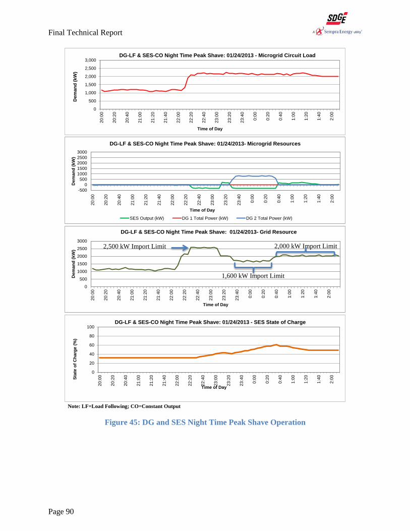
Final Technical Report
Page 90
Note: LF=Load Following; CO=Constant Output
Figure 45: DG and SES Night Time Peak Shave Operation
0
500
1,000
1,500
2,000
2,500
3,000
20
:00
20
:20
20
:40
21
:00
21
:20
21
:40
22
:00
22
:20
22
:40
23
:00
23
:20
23
:40
0:0
0
0:2
0
0:4
0
1:0
0
1:2
0
1:4
0
2:0
0
Dem
an
d (
kW
)
Time of Day
DG-LF & SES-CO Night Time Peak Shave: 01/24/2013 - Microgrid Circuit Load
0
20
40
60
80
100
20
:00
20
:20
20
:40
21
:00
21
:20
21
:40
22
:00
22
:20
22
:40
23
:00
23
:20
23
:40
0:0
0
0:2
0
0:4
0
1:0
0
1:2
0
1:4
0
2:0
0
Sta
te o
f C
harg
e (
%)
Time of Day
DG-LF & SES-CO Night Time Peak Shave: 01/24/2013 - SES State of Charge
-500
0
500
1000
1500
2000
2500
3000
20
:00
20
:20
20
:40
21
:00
21
:20
21
:40
22
:00
22
:20
22
:40
23
:00
23
:20
23
:40
0:0
0
0:2
0
0:4
0
1:0
0
1:2
0
1:4
0
2:0
0
Dem
an
d (
kW
)
Time of Day
DG-LF & SES-CO Night Time Peak Shave: 01/24/2013- Microgrid Resources
SES Output (kW) DG 1 Total Power (kW) DG 2 Total Power (kW)
0
500
1000
1500
2000
2500
3000
20
:00
20
:20
20
:40
21
:00
21
:20
21
:40
22
:00
22
:20
22
:40
23
:00
23
:20
23
:40
0:0
0
0:2
0
0:4
0
1:0
0
1:2
0
1:4
0
2:0
0
Dem
an
d (
kW
)
Time of Day
DG-LF & SES-CO Night Time Peak Shave: 01/24/2013- Grid Resource
1,600 kW Import Limit
2,500 kW Import Limit 2,000 kW Import Limit

Final Technical Report
Page 91
6 Deployment Scenarios
A deployment plan was developed for the optimized Microgrid solutions that were consistent
with the cost/benefit analysis of Task 5.1 report. The approach used was to extrapolate a large-
scale deployment of selected advanced distribution control (Microgrid) / DER strategies that
meet the requirements of the CBA of Task 5.1.
As stated in the Task 5.1 report, there are five identified solutions structured to enable maximum
benefits at specific load nodes on the SDG&E distribution network. The identified solutions are:
F. Large Microgrid (10 MW)
G. Medium Microgrid (4 MW)
H. Small Microgrid (1 MW)
I. Distributed Energy Resource (DER) solution (0.3 MW)
J. Residential solution (0.004 MW)
The benefits are derived from addressing issues specific to commercial and industrial (C&I)
consumer needs, communities challenged by high penetration of solar PV (HPV), weak points
(WP) in the network, end of circuit (EOC) challenges, and other (O) special needs (e.g. sports
venues, data centers, and hospitals). The benefits from addressing these challenges accrue to
certain beneficiaries:
Consumer (direct benefit to single consumers)
System (direct improvement in operations, system efficiency, and capital efficiency)
Societal (broadly applied benefits to many consumers)
This CBA resulted in 28 identified solutions in two phases as presented in Table 12 and Table 13
respectively. The 28 identified solutions include:
10 MW Microgrid: Quantity = 2
1 MW Microgrid: Quantity = 8
DER Solutions (300 kW): Quantity = 18
The deployment plan covers eight years in two Phases:
Phase 1: years 0 through 2; 10 identified solutions, all DER solutions
Phase 2: years 3 through 7; 18 identified solutions; 2 large Microgrids, 8 small
Microgrids, and 8 DER solutions

Final Technical Report
Page 92
Table 12: Phase 1 Identified Solutions at Key Load Nodes
Table 13: Phase 2 Additional Identified Solutions at Key Load Nodes
Zip CodeEstimated
Demand (MW)
Nodal
Strategic
Priority Score
Benefit Characteristic
SolutionViable Solution Fit MW
91932 11.36 5.70 Weak Point DER ( D ) 0.3
91933 11.36 5.70 Weak Point DER ( D ) 0.3
91942 13.20 4.55 Weak Point DER ( D ) 0.3
91942 13.18 4.55 Weak Point DER ( D ) 0.3
92071 11.18 3.80 Weak Point DER ( D ) 0.3
92121 14.00 4.55 End of Circuit DER ( D ) 0.3
92122 11.78 6.45 Weak Point DER ( D ) 0.3
92122 11.78 4.55 Weak Point DER ( D ) 0.3
92130 14.50 4.55 Weak Point DER ( D ) 0.3
92086 2.51 5.70 End of Circuit DER ( D ) 0.3
Zip CodeEstimated
Demand (MW)
Nodal
Strategic
Priority Score
Benefit Characteristic
SolutionViable Solution Fit MW
92019 13.20 1.90 Weak Point DER ( D ) 0.3
92026 12.59 1.90 Weak Point DER ( D ) 0.3
92027 12.97 3.80 High Penetration PV Small Microgrid ( C ) 1.0
92029 11.34 3.80 High Penetration PV Small Microgrid ( C ) 1.0
92040 15.88 1.90 High Penetration PV Small Microgrid ( C ) 1.0
92064 13.38 5.40 High Penetration PV Small Microgrid ( C ) 1.0
92069 15.69 1.90 Weak Point DER ( D ) 0.3
92111 13.65 1.90 Weak Point DER ( D ) 0.3
92121 14.00 4.55 Commercial & Industrial Large Microgrid ( A ) 10.0
92121 14.00 1.90 Weak Point DER ( D ) 0.3
92123 27.10 5.30 Commercial & Industrial Large Microgrid ( A ) 10.0
92126 13.34 1.90 Weak Point DER ( D ) 0.3
92126 13.34 1.90 High Penetration PV Small Microgrid ( C ) 1.0
92128 11.96 1.90 Weak Point DER ( D ) 0.3
92128 11.25 5.55 High Penetration PV Small Microgrid ( C ) 1.0
92130 14.50 4.55 High Penetration PV Small Microgrid ( C ) 1.0
92131 13.35 3.80 High Penetration PV Small Microgrid ( C ) 1.0
92131 13.35 1.80 Weak Point DER ( D ) 0.3

Final Technical Report
Page 93
CBA for SDG&E deployment - The cost/benefit analysis result for the entire 150 load nodes is
presented above in Section 5. In contrast, the Phase 1 and Phase 2 CBA results are presented
here.
Table 14: Phase1 and 2 Cost/Benefit Analysis
Benefits Annual Benefits 20-Year Present
Value
Consumer Benefits $4,824,972.75
System Benefits 14,557,285
Societal Benefits 372,702.34
$19,754,960 $152,570,785
Capital Cost Capital Cost
C&I $32,978,087
HPV 14,656,357
WP 5,957,654
EOC 744,707
Other -0-
$54,336,804
Utility Equity Portion of Capital
Expense 50.0%
Utility Equity Spend $27,168,402 $19,337,194
First Year O&M Cost First Year O&M
Cost
C&I $7,996,000
HPV 2,012,569
WP 5,440,000
EOC 680,000
Other $-
$16,128,569 $124,563,568
First Year Federal ITC First Year
Federal ITC
C&I $3,241,832
HPV 2,012,569
WP 1,527,518
EOC 190,940
Other $-
$6,972,859 $4,962,954
NPV Benefit w/o Federal ITC
$8,670,022
NPV Benefit w/ Federal ITC
$13,632,976
Number of Solutions
28
Capital Cost
$54,336,804
Thus, Phase 1 and 2 (together) represent a total net present value (NPV) benefit of nearly $9
million after all capital costs and O&M costs are covered.
The 28 identified Solutions can be found in 22 load nodes. Several load nodes required more
than one identified Solution to deliver the maximum benefits. Table 14 presents these findings.
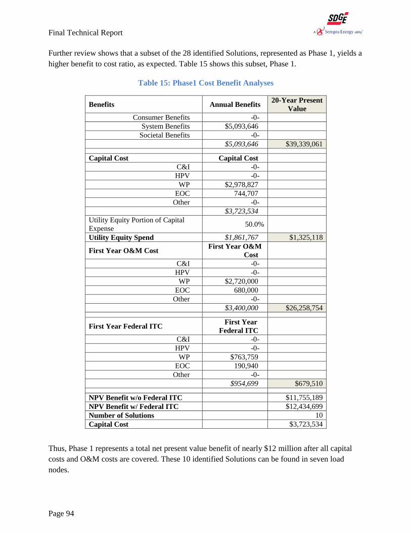
Final Technical Report
Page 94
Further review shows that a subset of the 28 identified Solutions, represented as Phase 1, yields a
higher benefit to cost ratio, as expected. Table 15 shows this subset, Phase 1.
Table 15: Phase1 Cost Benefit Analyses
Benefits Annual Benefits 20-Year Present
Value
Consumer Benefits -0-
System Benefits $5,093,646
Societal Benefits -0-
$5,093,646 $39,339,061
Capital Cost Capital Cost
C&I -0-
HPV -0-
WP $2,978,827
EOC 744,707
Other -0-
$3,723,534
Utility Equity Portion of Capital
Expense 50.0%
Utility Equity Spend $1,861,767 $1,325,118
First Year O&M Cost First Year O&M
Cost
C&I -0-
HPV -0-
WP $2,720,000
EOC 680,000
Other -0-
$3,400,000 $26,258,754
First Year Federal ITC
First Year
Federal ITC
C&I -0-
HPV -0-
WP $763,759
EOC 190,940
Other -0-
$954,699 $679,510
NPV Benefit w/o Federal ITC
$11,755,189
NPV Benefit w/ Federal ITC
$12,434,699
Number of Solutions
10
Capital Cost
$3,723,534
Thus, Phase 1 represents a total net present value benefit of nearly $12 million after all capital
costs and O&M costs are covered. These 10 identified Solutions can be found in seven load
nodes.

Final Technical Report
Page 95
Lessons from the Results
As expected, the smaller, higher priority set of solutions represented in Phase 1 yielded a
higher total net present value benefit, based on a smaller cost for these 10 solutions. It is
interesting to note that this highest value set consists of two EOC and eight WP
characteristics solved with DER solutions.
In the subsequent 18 solutions that represent the balance of Phase 2, there is a wide
variety of solutions employed. The variety of solutions gives SDG&E the opportunity to
compare performance in solving the characteristic issues being addressed. This set also
represents the next highest benefit cost ratios of the high priority load nodes.
Since the Phase 1 NPV Benefits were $12 million and the Phase 2 NPV Benefits were $9
million, one could say that the additional 18 solutions reduced the NPV Benefits by $3
million. This trend would suggest that seeking more than 28 solutions at the 22 load
nodes in the SDG&E territory would not likely generate sufficient benefits to justify the
capital and O&M costs.
The largest cost factors in the cost/benefit analysis that affected the benefit to cost ratio
the most were found in the O&M costs: natural gas fuel costs and finance payments.
These two costs create the largest sensitivity to the benefit cost ratio, and hence, the
cost/benefit analysis.
Financials – Technology Implementation - With the staged deployment as outlined in Section
4, the Phase 1 and 2 financial trend is shown in Figure 46. The proposed deployment plan
becomes cash positive in the sixth year. The graph clearly shows the major effect of the
operations and maintenance (O&M) costs, where fuel costs and loan payment constitute 80% to
83% of the O&M expense. Thus, driving the cost of fuel and loan payments down will improve
the business case.
Figure 46: Cash Flow for the Proposed Deployment Plan
$(10,000,000)
$(5,000,000)
$-
$5,000,000
$10,000,000
$15,000,000
$20,000,000
$25,000,000
$30,000,000
0 1 2 3 4 5 6 7 8 9 1011121314151617181920
Year
AnnualBenefits,Costs,andCashflow
AnnualBenefits AnnualEquitySpend
AnnualO&MExpense CashFloww/oITC

Final Technical Report
Page 96
7 Lessons Learned and Key Findings
Lessons Learned
The Microgrid demonstration proved to be a challenging project due to the complexity of
integrating new systems to the distribution network that could impact customers, reliance on
other projects for integration, the use of newly emerging technologies and systems, and
environmental requirements.
The team first identified the complexities during the use case development phase of the project.
The key stakeholders identified specific constraints with the existing systems and utility
processes which drove some key elements of the system architecture for the demonstration. The
use case process also demonstrated that Microgrids impact nearly all the departments within the
utility. It became clear that the approach that would be implemented for the demonstration
would be a first step toward the ability to integrate Microgrids but a more comprehensive
enterprise strategy would need to be developed if Microgrids were to be employed as a common
resource in the service territory.
The Microgrid project leveraged two existing diesel generators for the project. The team initially
assumed that this resource would be the most straight forward resource for integration and
operation. Two major issues had to be addressed for the generators 1) the existing controls were
inadequate for the project, and 2) the environmental requirements were more onerous than
expected. The control system had to be upgraded to support the planned modes of operation and
remote control of the units. In addition, the control interface had to include a method for the
Distribution Operators to have a level of control over the units in terms of paralleling to the grid
in a safe manner and disconnecting the generator in the case a fault on the circuit. To address the
emission requirements, the units were retrofit with a state-of-the-art emissions system that met
the Tier 4 emissions level required for the maximum annual hours of operation. Even while
meeting the most stringent standard for emissions, the generators had significant restrictions on
annual (200 hours/year), monthly, weekly and daily hours of operation, as well as time of day
restrictions. An additional constraint was associated with the noise coming from the generators.
To mitigate the noise issues, baffles were installed on the generators air intake, ventilation
louvers and exhaust systems, a “sound” wall was constructed on one side of the Microgrid Yard
that was facing the closest customer (~ 1,000 feet away), and advance customer notice of
operation was required.
For this project, the storage component proved to be quite challenging. Part of the challenge was
that the Microgrid storage unit was one of the first energy storage units purchased by the utility.
The Project team had to develop a specification and an RFP for the procurement. During the
procurement process, it was learned that the storage systems available at the time were basically
custom units and that few vendors could provide a turnkey solution without teaming with another
company. Vendors were either able to provide the storage or the power electronics but not both.
The procurement process for the Microgrid project took much longer than expected. The RFP
released at the early stages of the project resulted in the selection of a flow battery technology.

Final Technical Report
Page 97
A contract was never signed as the vendor had some difficulties in scaling their solution while
maintaining their efficiency. SDG&E worked with the vendor with support from EPRI to try to
resolve the performance issues but ultimately the procurement was canceled. A second RFP was
issued and this time a lithium ion technology was selected. The implementation schedule for the
selected storage unit was approximately a year. Due to the desert climate of the Microgrid
project, the vendor had to add air conditioning to the storage containers and the PCS to maintain
the appropriate operating temperatures in the storage system enclosures. This unexpectedly
proved to be an issue with the reliability of the units. Failures of the air conditioning units
caused the batteries and the PCS to shut down. The controls protected the system so the
equipment was not damaged when to the high temperature events occurred. The cooling issue
was addressed and eventually resolved during the course of the demonstration.
The implementation of FLISR relied on installing a new distribution management system being
deployed by the utility. The ability to program and simulate the FLISR operations on the
Microgrid Circuit was delayed until the end of the demonstration due to the schedule and
requirements of the larger Advanced Distribution Management System project. However, the
Microgrid Circuit was the circuit used to develop the test cases and validate FLISR operations
for the new distribution management system.
The PDLM system integration and deployment was expected to be challenging at the beginning
of the project and this proved to be the case as the project was executed. The use case results
from the beginning of the project were used to develop an RFP for the system. A vendor that
had formed a team to provide a turnkey solution was selected. The vendor had a base software
solution for demand response that was modified to meet the pricing functional requirements for
the Microgrid project. At first, this appeared to be a benefit to meeting the project schedule;
however the schedule was a challenge for the project. It should be noted that the PDLM portion
of the demonstration was co-funded by the California Energy Commission contract that had a
shorter period of performance than the DOE funded portion of the demonstration. The
implementation of the PDLM software required a security validation process before it could be
approved to be operated along with the “production” systems operated by the utility. This
process had a major impact on the schedule.
Another challenge to the PDLM implementation was the recruitment of customers. Many
customer outreach and recruitment events were held in the community to entice residential
customers to have the HAN systems installed in their homes and participate in non-tariff based
demand response events over the course of a one year period. The target for the number of
participants was 125; however a total of 65 were enrolled and participated. By the time the
system was installed and accepted for operation, the demonstration project schedule was near the
end and many of the demand response events had to be conducted during a non-summer time
period which significantly reduced the real demand response impact of weather based loads (i.e.
air conditioning).
A significant effort was placed on the development of a Microgrid Controller for the
demonstration project. The challenge for the Microgrid Controller was that there was not an

Final Technical Report
Page 98
existing product in the market that could easily be acquired and modified to meet the needs of
the project. A decision was made to work with the vendor selected for the new Distribution
Management System to leverage this work to provide a Microgrid Controller. While this
initially appeared to be a benefit to the project it became clear that the timeline for product
development and controller objectives by the vendor did not align well with the demonstration
project. Furthermore, the security testing requirements to place the controller into the utility’s
“production” environment pushed the delivery schedule out further. It was finally decided to
develop a project-specific application to provide a consolidated view of the Microgrid Resources
referred to as the Microgrid Visualizer. The Microgrid Visualizer facilitated the planned
Microgrid demonstrations by providing a method to easily operate the systems from a single
screen, schedule equipment, monitor operations, and collect data. The Microgrid Visualizer was
successfully used to support the demonstrations, including islanding operations, but is not a
standalone and fully-automated control system.
Finally, another issue that had to be addressed for the demonstration project was the load profile
of the Microgrid Circuit. The load profile is very unconventional where the peak load occurs at
night when the water district and agricultural customers operate pumps for an extended period of
time. From a technical perspective this is not an issue for a Microgrid to appropriately meet its
peak load, economic, and reliability objectives. However, the environmental and other
constraints identified above related to the allowed generator time of use, prevented the generators
from fully addressing the peak load management objectives of the project. In order to address
these constraints, demonstrations were designed and conducted to address the peak load
management through a sequence of operation using a combination of the DG units and the
storage system. For example, because the generators could not operate after 1:00 AM, any
demonstrations that occurred after that time had to rely on the storage system only.
Key Findings
The aspects of the project considered to be unique and to potentially advance the knowledgebase
of Microgrids were:
Development of an architecture and operational processes for utility-based
Microgrids
The Microgrid demonstration provided key lessons about the architecture that was
suitable for this Microgrid demonstration. However, the demonstration did not produce
an architecture that is easily scalable for deployment for the entire service territory. A
scaled up deployment in the service territory will require a comprehensive enterprise
strategy and additional automation capabilities through the distribution management
system, distributed Microgrid Controllers, or a distributed energy resource management
system.

Final Technical Report
Page 99
Identification and validation of key functions of energy storage systems within a
Microgrid
Functionality of the energy storage system within the Microgrid took place in many
forms. The key modes of operation: constant charge and discharge, peak shaving, and
reactive power were leveraged to accommodate many functions based on various
triggering events. These included circuit load management, optimization of generator
loading, demand response support, arbitrage, and VAr control in both grid connected and
island mode operations. In addition, experience was gained with respect to the need for
energy storage management where future operational requirements are identified and
approaches are developed so that the storage is at the desired state of charge in time to
execute the desired future mode of operation. Due to the current high capital cost of
storage systems, the storage system must contribute to several system benefits in order to
be cost effective. The demonstration also showed that the arbitrage operations do not
derive a high economic value for the Microgrid but should be taken into account as a
secondary consideration when planning storage system operations. The demonstration
also showed that having four quadrant operation capabilities (injecting or consuming
VArs while charging or discharging) was beneficial to the flexibility of operation to
support Microgrid activities.
Develop and implement a pricing-based strategy to affect the operation of resources
within a Microgrid
The team successfully developed a pricing model that was used by multiple Microgrid
resources to influence and affect operations, particularly reducing demand to provide
demand management resources to support the microgrid circuit load. The idea to
implement pricing was to have a market-based trigger that is used to influence Microgrid
operations. In the microgrid demonstration, pricing signals influenced demand response
with the objective of reducing the customer load. Demonstrations were conducted where
a wholesale price was calculated based on a weighted average of Microgrid resource
contributions to the planned energy supply of the Microgrid for each hour of the day.
These prices where then converted to a “simulated” retail price that was presented to
customer’s in home display units and HAN devices. The HAN devices responded as
programmed during these pricing event demonstrations. As discussed in the storage
system findings, the cost of energy was taken into account when charging the storage
system. This allowed for the cost of energy being provided to the Microgrid when the
storage unit was discharging to be accurately accounted. Thus, during times of high
whole costs, a storage unit that had been charged during the off-peak low cost time
periods could be used to reduce the cost of energy delivered to the Microgrid during peak
time periods. The demonstration showed that this pricing-based strategy could
effectively be used as a control signal for Microgrid Operations.

Final Technical Report
Page 100
Determine if there are approaches to utilizing demand response resources in a
manner similar to generation in terms of dispatchability, reliability, and localization
The team envisioned that the use of home area networks combined with a central demand
response control system could be used in a Microgrid to manage the demand response
resource in a manner similar to the generators or the storage system. In order to
accomplish this, demand response needs to be controllable, predictable, and repeatable.
This proved to be challenging for the demonstration due to the resource load forecast
model used, the post event estimating approached employed, the small loads being
managed (mainly plug load controllers), and the small population of customers in the
program. The project did successfully implement a demand response model that could
execute demand response events for a targeted area of the service territory down to a
section of a specific circuit. The demand response was not a major factor in Microgrid
resource planning during the Microgrid Optimization Phase of the project due to its low
capacity impact. Demand response has been identified as an area of further work that has
the potential to be improved for both Microgrid applications and overall demand response
activities.
Demonstrate the ability to routinely operate multiple Microgrid Resources through
a consolidated monitoring and control interface
Routinely operating utility-owned generation and energy storage systems on the
distribution network is a new concept for utility distribution system operators. In
addition, these devices do not currently have a communication standard such as DNP3
that allows for a more straight forward integration to a typical SCADA system. The units
integrated to the Microgrid offered a Modbus protocol for communications and control.
In addition, these types of resources have unique operating characteristics and control
sequences can be vendor-specific. In order to effectively operate these systems, a
Microgrid Visualizer was developed and implemented that provided a consolidated
interface to the equipment controls and monitoring. The Visualizer allowed for control of
the Microgrid resource both from within the Microgrid yard (control van) and remotely
from SDG&E offices in San Diego. This system also provided the function of data
collection and archiving for project reporting and analysis.
Demonstrate seamless planned island operations on a circuit without affecting
customers
One of the highlights of the Demonstration project was the ability to effectively island the
entire Microgrid supporting more than 600 customers. The islanding demonstrations
transitioned into and out of the island mode without affecting the quality of service to the
customers (seamless transitions without an outage or flicker). The island demonstrations
evaluated the island operations with the DG units only, the DG units operating with the
SES in both charge and discharge modes, and the DG units operating with the SES unit

Final Technical Report
Page 101
providing a majority of the reactive power requirements. All demonstrations were
successful and demonstrated the stated operational objectives.
Additionally, the Microgrid was operated in island operation twice during the contract
period to provide service to customers who would have otherwise had an extend loss of
service.
o The first event took place on June 6, 2012 for a planned outage for the Borrego
Springs community so that a new commercial 26 MW solar project could be
safely interconnected to SDG&E’s system. The outage began at 10:00 PM and
lasted for approximately 5 ½ hours supplying energy to a total of 2,128
customers. This was a pre-planned operation in which the Microgrid was
temporarily re-configured to service all three of the circuits at the substation.
o The second event took place on September 6, 2013 when severe weather of high
winds, heavy rain and a lighting storm caused an unplanned outage of service to
the entire substation. This manual black start operation primarily used the
generators which were operated continuously on September 6 from 16:48 PM to
3:10 PM on September 7. As sections of the circuits were cleared or repaired,
additional customers were energized as presented in the following table:
Date Time Customers with Service
9/6/2013 2:20 PM 0 – Start of outage
9/6/2013 6:50 PM 162 – Powered by Microgrid
9/6/2013 7:50 PM 529 – Powered by Microgrid
9/7/2013 7:25 AM 754 – Powered by Microgrid
9/7/2013 8:33 AM 1,056 – Powered by Microgrid
9/7/2013 2:00 PM All – All repairs complete and grid service resumes
Utilize the outcomes of the demonstration to identify future cost-effective
deployments of Microgrids in the service territory - The lessons learned and the
quantified benefits from the Microgrid demonstration were used to identify other
potential cost effective Microgrid applications in the SDG&E service territory.
Applications were identified where there is a high potential to improve existing
distribution operations and classified with their associated characteristics as follows:
Commercial and Industrial Consumers (C&I)
o Behind the meter
o High reliability requirement
o Third-party finance of projects
o Community-level
o Increasing use of PV
o Potential low cost of capital

Final Technical Report
Page 102
Communities with Challenges with high Penetration of Solar PV (HPV)
o Isolate one or more stability issues
o Adapt community or network to stability issues
Weak Points in the Distribution Network
o Topology
o Unexpected growth
o Nodal issues
End of Circuit (EOC)
o Voltage support
o Conservation voltage reduction
o Avoid re-conductor on load growth
Other (O)
o Sites with special needs (sports venues, data centers, hospitals, etc.)
The key findings from the cost benefit analysis are that potential deployment of cost-effective
Microgrids and DER are not as broad and deep as expected. A total of 28 cost-effective
applications were identified:
10 MW Microgrid: quantity = 2
1 MW Microgrid: quantity = 10
300 kW DER solutions: quantity = 18
For utility-based Microgrids, it is important to structure a selection process that is based on the
following:
Benefit Characteristic Solutions need to be tied to the needs of the territory’s electric
system
Strategic Priorities need to be identified and ranked
Identified Solutions need to be designed to deliver the benefits identified in the Benefit
Characteristic Solutions
Characterize the territory, or network topology, to link electric loads with locations and a
consumer population of likely participants
The analysis needs to be based on a life cycle cost model that must include capital costs,
utility integration costs, and equipment O&M expenses
It is important to develop a cost benefit selection structure that enables a criteria based selection
using the best site solution-benefit pairings to ensure the maximum economic returns.
[End of Report]