THE CREDIT-DEFAULT SWAP MARKET:

Is Credit Protection Priced Correctly?

Francis A. Longstaff

Sanjay Mithal

Eric Neis

Initial version: December 2002.Current version: August 2003.

Francis Longstaff is with the Anderson School at UCLA and the National Bureau ofEconomic Research. Sanjay Mithal is a Director in the North American structuringgroup at Deutsche Bank in New York. The views in this paper are his own, anddo not represent those of Deutsche Bank. Eric Neis is a Ph.D. student at theAnderson School at UCLA. Corresponding author: Francis Longstaff, email address:francis.longstaff@anderson.ucla.edu. We are grateful for valuable comments andassistance from Dennis Adler, Darrell Duffie, Joseph Langsam, Jun Liu, Jun Pan,Eduardo Schwartz, Jure Skarabot, Soetojo Tanudjaja, and Ryoichi Yamabe. Allerrors are our responsibility.

USC FBE FINANCE SEMINARpresented by Francis LongstaffFRIDAY, October 24, 200310:30 am - 12:00 pm; Room: JKP-204

ABSTRACT

We examine the pricing of credit protection in the rapidly growing credit-default swap market using an extensive data set provided by Citigroup.We fit a reduced-form model to corporate bond yields and solve for thecredit-default swap premia they imply. We compare these implied credit-default swap premia to actual market premia. Implied premia tend tobe much higher than market premia. The differences are related tomeasures of Treasury specialness, corporate bond illiquidity, and couponrates of the underlying bonds, suggesting the presence of important tax-related and liquidity components in corporate spreads. Both the credit-derivatives and equity markets tend to lead the corporate bond market.

1. INTRODUCTION

Credit derivatives are rapidly becoming one of the most successful financial innova-tions of the past decade. The British Bankers’ Association estimates that from atotal notional amount of $180 billion in 1997, the credit-derivatives market grew morethan tenfold to $2.0 trillion by the end of 2002. Furthermore, the British Bankers’Association forecasts that the total notional amount of credit derivatives will reach$4.8 trillion by the end of 2004. In a November 19, 2002 speech before the Councilon Foreign Relations, Federal Reserve Chairman Alan Greenspan praised the credit-derivatives market for its role in allowing banks and other financial institutions tohedge credit risk.

The nearly-explosive growth of this market, however, has also been accompaniedby controversy. In particular, concerns have been raised recently about whether creditprotection is priced fairly in the credit-derivatives market. For example, some claimthat hedge funds have artificially driven up the price of credit protection in an effort toinduce the ratings agencies to downgrade specific firms. From theWall Street Journalon December 5, 2002,

“Among those sounding the alarm that savvy players are whipsawing themarket to their advantage is William Gross, managing director of PacificInvestment Management Co., or Pimco, the largest bond investor in the U.S.. . . critics such as Mr. Gross [argue that] hedge funds often use both thebond market and the credit-derivatives market to push companies that arebarely investment grade into speculative grade territory.”

On the other hand, reports that a number of credit-protection sellers have experiencedlosses and are scaling back or exiting the market suggest that some credit protectionmay have been sold too cheaply. From the Economist on January 18, 2003,

“Frank Ronan, global head of credit at Swiss Re, a reinsurer, says that his in-dustry absorbed a ‘massive amount of risk in a relatively short period of time’and, unfortunately, did it ‘right at the end of a bull market.’ So far, SwissRe, SCOR, a French reinsurer, and America’s Chubb Corporation have an-nounced losses on credit-derivative products. Having been bitten once, insur-ers are getting shy of selling credit protection. . . . Swiss Re, said this weekthat the company is winding down its credit-derivatives book. Dealers say thatsome big sellers of protection–Ambac Financial Group, Financial SecurityAssurance, MBIA, General RE and Zurich Financial Services Group–havereduced their activities.”

1

Motivated by these issues, this paper conducts an in-depth empirical examinationof the pricing of credit protection within the credit-default swap market. Credit-default swaps are the most common type of credit derivative. In a credit-defaultswap, the party buying protection pays the seller a fixed premium each period untileither default occurs or the swap contract matures. In return, if the underlying firmdefaults on its debt, the protection seller is obligated to buy back from the buyer thedefaulted bond at its par value. Thus, a credit-default swap is similar to an insurancecontract compensating the buyer for losses arising from a default. A key aspect of ourstudy is the use of an extensive data set on credit-default swap premia and corporatebond prices provided to us by the Global Credit Derivatives desk at Citigroup. Thisproprietary data set includes weekly market quotations for a broad cross section offirms that are actively traded in the credit-derivatives market. Using this data, wecan directly examine whether the pricing of credit protection in the credit-derivativesmarket is consistent with the pricing of corporate bonds.

In conducting this analysis, we first develop a closed-form model for credit-defaultswap premia using a variant of the familiar Duffie and Singleton (1999) framework.In this reduced-form model, the default intensity follows a square-root process. Foreach firm, we estimate the parameters of the model and the implied intensity processby fitting to a cross section of corporate bond prices with maturities straddling thefive-year horizon of the credit-default swaps in the sample. Substituting these valuesinto the model gives the default swap premia implied by the corporate bond market.These model values are then compared directly to the actual values observed in thecredit-default swap market. To illustrate our approach, we apply it to a detailed casestudy of Enron. The approach is then extended to all of the firms in the sample.

A number of important results emerge from the analysis. We find that for almostall firms in the sample, the cost of credit protection in the credit-default swap market issignificantly less than the cost implied by the firm’s bonds. There are several possibleinterpretations of this finding. Foremost among these is the possibility that corporatespreads may include credit, tax-related, and liquidity components. In pricing creditderivatives, however, only the credit component of the corporate spread is relevant.Thus, the difference between the model and market values for the credit-default swappremium may represent the tax and liquidity components of corporate spreads. Toexplore this, we regress the pricing differences on measures of Treasury bond richnessor specialness, measures of individual corporate bond illiquidity, and the coupon ratesof the corporate bonds. The results strongly support the view that corporate spreadsare affected by the differential State tax treatment of corporate bonds, the generalliquidity or specialness of Treasury bonds, and the illiquidity of individual corporatebonds. We conduct a number of robustness checks for the results and show that theyare not explained by modeling error, the frequent use by market participants of theswap curve as the discounting curve, swap counterparty default risk, or the costs ofshorting corporate bonds.

2

To explore further how credit protection is priced in the credit-derivatives market,we use a vector-autoregression framework to examine the lead-lag relations betweencredit-default swap premia, corporate bond spreads, and equity returns. The resultsstrongly support the hypothesis that the credit-default swap market leads the corpo-rate bond market by at least a week. Surprisingly, the credit-default swap market alsoappears to lead the equity market for a sizable fraction of the firms in the sample.These results have many potential implications for the role of the credit-derivativesmarket in price discovery and information aggregation.

The literature on credit derivatives is growing rapidly. Important theoretical workin the area includes Jarrow and Turnbull (1995, 2000), Longstaff and Schwartz (1995a,b), Das (1995), Duffie (1998, 1999), Lando (1998), Duffie and Singleton (1999), Hulland White (2000, 2001), Jarrow and Yildirim (2001), Das, Sundaram, and Sundaresan(2003), and many others. There are also several recent empirical studies of the pricingof credit-default swaps including Cossin, Hricko, Aunon-Nerin, and Huang (2002),Houweling and Vorst (2002), and Zhang (2003). This paper differs fundamentally fromthe first two of these studies in that our approach is based on a fully-parameterizedreduced-form model. Furthermore, our focus is on how well the market prices creditprotection rather than on comparing alternative models. Our paper also differs fromZhang in that we use corporate bond data to calculate the implied price of creditprotection and then compare it to the market price of credit protection.

The remainder of this paper is organized as follows. Section 2 provides a briefintroduction to credit-default swaps and the credit-derivatives market. Section 3presents the credit-default swap model. Section 4 presents a case study of Enron.Section 5 examines whether credit-default swaps and corporate bonds are priced con-sistently with each other. Section 6 examines the time-series and cross-sectional struc-ture of the pricing differences. Section 7 considers a number of alternative explanationsfor the results. Section 8 examines the lead-lag relations among the swap, bond, andequity markets. Section 9 summarizes the results and presents concluding remarks.

2. CREDIT-DEFAULT SWAPS

Credit derivatives are contingent claims with payoffs that are linked to the credit-worthiness of a given firm or sovereign entity. The purpose of these instruments is toallow market participants to trade the risk associated with certain debt-related events.Credit derivatives widely used in practice include total-return swaps, spread options,and credit-default swaps.1 In this paper, we focus exclusively on the latter since theyare the predominant type of credit derivative trading in the market.2

1Credit-default swaps on a portfolio of bonds, sometimes called portfolio credit-defaultswaps, also exist. For example, see Fitch IBCA, Duff and Phelps (2001).

2The British Bankers’ Association (2002) reports that single-name credit-default swaps

3

The simplest example of a single-name credit-default swap contract can be il-lustrated as follows. The first party to the contract, the protection buyer, wishes toinsure against the possibility of default on a bond issued by a particular company. Thecompany that has issued the bond is called the reference entity. The bond itself isdesignated the reference obligation. The second party to the contract, the protectionseller, is willing to bear the risk associated with default by the reference entity. Inthe event of a default by the reference entity, the protection seller agrees to buy thereference issue at its face value from the protection buyer. In return, the protectionseller receives a periodic fee from the protection buyer. This fee, typically quoted inbasis points per $100 notional amount of the reference obligation, is called the defaultswap premium. Once there has been a default and the contract settled (exchange ofthe bond and the face value) the protection buyer discontinues the periodic payment.If a default does not occur over the life of the contract, then the contract expires atits maturity date.

As a specific example, suppose that on January 23, 2002, a protection buyer wishesto buy five years of protection against the default of the Worldcom 7.75 percent bondmaturing April 1, 2007. The buyer owns 10,000 of these bonds, each having a faceamount of $1,000. Thus, the notional value of the buyer’s position is $10,000,000. Thebuyer contracts to buy full protection for the face amount of the debt via a single-namecredit-default swap with a 169 basis point premium. Thus, the buyer pays a premiumof A/360× 169, or approximately 42.25 basis points per quarter for protection, whereA denotes the actual number of days during a quarter. This translates into a quar-terly payment of A/360 × $10, 000, 000 × .0169 = A/360 × $169, 000. If there is adefault, then the buyer delivers the 10,000 Worldcom bonds to the protection sellerand receives a payment of $10,000,000. If the credit event occurs between default swappremium payments, then at final settlement, the protection buyer must also pay tothe protection seller that part of the quarterly default swap premium that has accruedsince the most recent default swap premium payment.3 Credit events that typicallytrigger a credit-default swap include bankruptcy, failure to pay, default, acceleration,a repudiation or moratorium, or a restructuring.

In the most general credit-default swap contract, the parties may agree that anyof a set of bonds or loans may be delivered in the case of a physical settlement (asopposed to cash settlement, to be discussed below). In this case, the reference issueserves as a benchmark against which other possible deliverable bonds or loans mightbe considered eligible. In any case, the deliverable obligations are usually specifiedin the contract. It is also possible, however, that a reference obligation may not bespecified. In this case, any senior unsecured obligation of the reference entity may

are the most popular type of credit derivative, representing nearly 50 percent of thecredit-derivatives market.3Worldcom filed for bankruptcy on July 21, 2002.

4

be delivered. Cash settlement, rather than physical settlement, may be specified inthe contract. The cash settlement amount would either be the difference betweenthe notional and market value of the reference issue (which could be ascertained bypolling bond dealers), or a predetermined fraction of the notional amount. Note thatbecause the protection buyer generally has a choice of the bond or loan to deliver inthe event of default, a credit-default swap could include a delivery option similar tothat in Treasury note and bond futures contracts.4

Since credit-default swaps are OTC contracts, the maturity is negotiable, andmaturities from a few months to ten years or more are possible, although five years isthe most common or liquid tenor in the market. In this paper, we focus on corporatesand financials where the greatest liquidity is in contracts with a five-year maturity.The notional amount of credit-default swaps ranges from a few million to more than abillion dollars, with the average being in the range of $25 to $50 million (J.P. Morgan(2000)). A wide range of institutions participate in the credit-derivatives market.Banks, security houses, and hedge funds dominate the protection-buyers market, withbanks representing about 50 percent of the demand. On the protection-sellers side,banks and insurance companies dominate (British Bankers’ Association (2002)).

3. THE CREDIT-DEFAULT SWAP MODEL

In this section, we develop a simple closed-form model for valuing credit-default swapswithin the well-known reduced-form framework of Duffie (1998), Lando (1998), Duffieand Singleton (1999), and others. In particular, we model the default intensity as asquare-root process and provide explicit solutions for credit-default swap premia andcorporate bond prices.

Following standard notation, let rt denote the riskless rate and λt the intensityof the Poisson process governing default. Both rt and λt are stochastic, although weassume that they follow independent processes. As we show later, this assumptiongreatly simplifies the model, but has little effect on any of the empirical results. As inLando (1998), we make the assumption that a bondholder recovers a fraction 1−w ofthe par value of the bond in the event of default.

Given the independence assumption, we do not actually need to specify the risk-neutral dynamics of the riskless rate to solve for credit-default swap premia and cor-porate bond prices. We require only that these dynamics be such that the value of ariskless zero-coupon bond D(T ) with maturity T be given by the usual expression,

D(T ) = E exp −T

0

rt dt . (1)

4For an in-depth discussion of this feature, see Mithal (2002).

5

To specify the risk-neutral dynamics of the intensity process λt, we assume that

dλ = (α− βλ) dt + σ√λ dZ, (2)

where α, β, and σ are positive constants, and Zt is a standard Brownian motion.These dynamics allow for both mean reversion and conditional heteroskedasticity incorporate spreads and guarantee that the intensity process is always nonnegative.Given these dynamics, standard results can be used to show that the probability thatdefault has not occurred by time T is

exp −T

0

λt dt , (3)

and that the density function for the time until default is

λt exp −t

0

λs ds dt. (4)

Following Duffie (1998), Lando (1998), Duffie and Singleton (1999) and others, itis now straightforward to represent the values of corporate bonds and the premium andprotection legs of a credit-default swap as simple expectations under the risk-neutralmeasure. Let c denote the coupon rate for a corporate bond, which for notationalsimplicity is assumed to pay coupons continuously. It is easily shown that the priceof this corporate bond CB(c, w, T ) can be expressed as

CB(c, w, T ) = E cT

0

exp −t

0

rs + λs ds dt

+ E exp −T

0

rt + λt dt

+ E (1− w)T

0

λt exp −t

0

rs + λs ds dt . (5)

The first term in this expression is the present value of the coupons promised by thebond, the second term is the present value of the promised principal payment, andthe third term is the present value of recovery payments in the event of a default.

Let s denote the premium paid by the buyer of default protection. Assumingthat the premium is paid continuously, the present value of the premium leg of acredit-default swap P (s, T ) can be expressed as

6

P (s, T ) = E sT

0

exp −t

0

rs + λs ds dt . (6)

Similarly, the value of the protection leg of a credit-default swap PR(w, T ) can beexpressed as

PR(w, T ) = E wT

0

λt exp −t

0

rs + λs ds dt . (7)

Setting the values of the two legs of the credit-default swap equal to each other andsolving for the premium gives

s =E w

T

0λt exp − t

0rs + λs ds dt

ET

0exp − t

0rs + λs ds dt

. (8)

If λt is not stochastic, the premium is simply λw. Even when λt is stochastic, however,the premium can be interpreted as a present-value-weighted-average of λtw. In general,because of the negative correlation between λt and exp(− t

0λs ds), the premium

should be less than the expected average value of λt times w.

Given the square-root dynamics for the intensity process λt, standard results suchas those in Duffie, Pan, and Singleton (2000) make it straightforward to derive closed-form solutions for the expectations in Eqs. (5), (6), and (7). Appendix A shows thatthe value of a corporate bond is given by

CB(c, w, T ) = cT

0

D(t) A(t) exp( B(t) λ ) dt +

D(T ) A(T ) exp( B(T ) λ ) +

(1− w)T

0

D(t) ( C(t) + H(t) λ ) exp( B(t) λ ) dt, (9)

where λ denotes the current (or time-zero) value of the intensity process, and where

7

A(t) = expα(β + φ)

σ2t

1− κ1− κeφt

2ασ2

,

B(t) =β − φσ2

+2φ

σ2(1− κeφt) ,

C(t) =α

φeφt − 1 exp

α(β + φ)

σ2t

1− κ1− κeφt

2ασ2+1

,

H(t) = expα(β + φ) + φσ2

σ2t

1− κ1− κeφt

2ασ2+2

,

φ = 2σ2 + β2,

κ = (β + φ)/(β − φ).

Similarly, Appendix A shows that the credit-default swap premium is given by

s =w

T

0D(t) ( C(t) + H(t) λ ) exp( B(t) λ ) dt

T

0D(t) A(t) exp( B(t) λ ) dt

. (10)

To provide some intuition about the credit-default swap premium, we note that in aninsightful paper, Duffie (1999) shows that the premium equals the fixed spread overthe riskless rate that a corporate floating rate note would need to pay to be able tosell at par. Thus, if both a firm and the Treasury issued floating rate notes tied to theriskless rate r, the fixed spread between the rates paid by the floating rate notes wouldequal s. It is important to observe, however, that this result does not extend to theyield spreads between corporate and Treasury fixed rate bonds. Duffie and Liu (2001)show that the spreads on fixed rate bonds can differ from spreads on floating ratesecurities. To a first order approximation, however, it is often useful to think of thecredit-default swap premium as being roughly equal to the yield spread of the referenceissue corporate bond over the yield of a Treasury bond with the same maturity dateand coupon rate. We will refer to the yield spread between corporate and Treasury

8

bonds with the same coupon rates and maturity dates as the constant-coupon spreadthroughout this paper.

With these closed-form solutions, our empirical approach will be to fit the modelto the prices of corporate bonds using Eq. (9), and then solve for the premiumimplied by the model using Eq. (10). The model-implied values of the premia arethen compared with actual market credit-default swap premia.

4. THE ENRON CASE STUDY

Before applying this approach to the entire sample, it is helpful to first illustrate howthe approach is implemented via a case study of Enron during the year leading upto its eventual default and Chapter 11 bankruptcy filing on December 2, 2001. Twoprimary types of Enron data are used in this case study: credit-default swap premiaand corporate bond yields.

The credit-default swap data used in this case study consist of bid and ask quota-tions for five-year credit-default swaps on Enron during the period from December 5,2000 to October 22, 2001. Quotations are available only on days when there is somelevel of liquidity in the market as evidenced either through trades or by active marketmaking by a dealer. For Enron, we have 31 observations during the sample period,corresponding to roughly a weekly frequency. As the point estimate of the credit-default swap premium, we use the midpoint of the bid and ask quotations. The dataare provided to us by the Global Credit Derivatives desk at Citigroup. We note, how-ever, that the data set includes quotations from a variety of credit-derivatives dealers.Thus, quotations should be representative of the entire credit-derivatives market.

Since the credit-default swaps in the sample have a five-year horizon, it wouldbe ideal if there was always a matching five-year bond available at each observationdate from which the probability of default could be determined. In reality, there areno Enron bonds that exactly match the five-year maturity of the credit-default swapsfor any of the observation dates in the sample. Even if there were, the possibilityof noise or measurement error in the bond price data would introduce volatility intothe estimate of the default probability. To address these two problems, we adopt thefollowing straightforward, and hopefully, more robust approach. Rather than focusingon a specific Enron bond, we use data from a set of bonds with maturities that bracketthe five-year horizon of the credit-default swap. The process used to identify thesebonds is described in Appendix B. This process resulted in a set of eight Enron bondswith maturities ranging from June 2003 to October 2007.5 These eight bonds are allfixed-rate senior unsecured dollar-denominated debt obligations of Enron and do not

5The maturity dates of the credit-default swaps associated with the first and last datesin the sample are December 5, 2005 and October 22, 2006. Thus, this set of bondshas maturities that bracket the maturity dates of the credit-default swap quotes in

9

have any embedded options. To mitigate the effects of illiquidity, only bonds that areregistered with the SEC are included in the set. The coupon rates for these bondsrange from 6.625 to 9.875 percent. We refer to this set of bonds as the bracketing set.The bond yield data are also obtained from a proprietary corporate bond databaseprovided by Citigroup. Given the well-documented measurement problems associatedwith corporate bond data, we conducted a number of robustness checks using data forthe bonds collected from the Bloomberg system to verify that our data are reliable.

Turning now to the estimation of parameters, we first need to identify the risklessdiscount function D(T ) for each observation date. This is done by collecting data forthe constant maturity six-month, one-year, two-year, three-year, five-year, seven-year,and ten-year Treasury rates from the Federal Reserve. We then use a standard cubicspline algorithm to interpolate these par rates at semiannual intervals. These par ratesare then bootstrapped to provide a discount curve at semiannual intervals. To obtainthe value of the discount function at other maturities, we use a straightforward linearinterpolation of the corresponding forward rates.

To estimate the parameters for the intensity process λt, we do the following. First,we pick trial values for the parameters α, β, and σ. For each of the 31 observationdates, we have yields for a subset (ranging from three to eight, and averaging four)of the Enron bonds in the bracketing set described above. Given the parameters, wesolve for the value of λt that results in the best root-mean-square fit of the model tothe bond yields for that date.6 We repeat this process for all 31 observation dates andcompute the root-mean-squared error over all of the 31 observation dates. We thenpick another trial value of the parameters, and repeat the entire process. Convergenceoccurs by searching over parameter values until the global minimum value of theoverall root-mean-squared error is obtained. Throughout this procedure, we hold therecovery percentage w constant at 50 percent.7 However, the estimation results arevirtually identical when other values of w are used.

This estimation approach has several key advantages. Foremost among these isthat by fitting to a cross section of bonds with maturities that bracket that of thecredit-default swap, we minimize the effect of any measurement error in individualbond prices on the results. In essence, by using a cross section of bonds, we attemptto “average out” the effects of idiosyncratic pricing errors in individual bonds.

This process results in estimates for the three parameters α, β, and σ of the risk-

the sample.6In doing this, we fit the market bond data to a discrete version of Eq. (9) that matchesthe actual semiannual timing of coupon payments (rather than assuming that couponsare paid continuously).

7A 50 percent recovery rate is consistent with the median value for senior unsecuredbonds reported in Duffie and Singleton (1999).

10

neutral dynamics as well as for the value of λt for each of the 31 observation dates inthe sample. The estimated dynamics of the intensity process are

dλ = (0.0054 − 0.0534 λ) dt + 0.0422√λ dZ. (11)

The overall root-mean-squared error from the fitting procedure is 7.1 basis points,which is small given the large variation in Enron spreads during the sample period.8

Fig. 1 plots the implied values of the intensity parameter λt for each of the 31observation dates. As shown, the implied probability of a default rises slowly fromabout 2.1 percent at the beginning of 2001 to about 3.0 percent near the end of August2001. Around the second week of October 2001, however, the implied probability of adefault increases rapidly and quickly exceeds a level of 5.0 percent. Table 1 providesa chronology of some of the events leading up to Enron’s bankruptcy. The chronologyshows that that the first indications of major financial problems at Enron surfaced inthe press around October 16, 2001. Enron’s debt was downgraded by Standard andPoor’s to B- on November 28, 2001, and to CC on November 30, 2001. Enron filedfor bankruptcy and defaulted on its debt on December 2, 2001. Note that the lastobservation in our sample is dated October 22, 2001.

Substituting the estimated parameters and values of λt into Eq. (10) now givesthe model-implied credit-default swap premia. Fig. 2 plots these implied premia alongwith the actual market premia. Near the beginning of 2001, the model and marketvalues are quite close to each other. During the middle of the year, however, theimplied premium is roughly 50 basis points higher than the market premium. Thispattern is reversed in September 2001 when the implied premium lags behind themarket premium. On average, the two premia are quite close. In particular, theaverage value of the implied premium is 186.1 basis points while the average valueof the actual premium is 173.6 basis points. The difference in means is 12.5 basispoints which is on the order of bid-ask spreads observed in the credit-default swapmarkets. The t-statistic for the difference in means is 1.79 which is not significant atthe five percent level (although it is significant at the ten percent level). These resultssuggest that the price of credit protection implied from Enron corporate bonds isslightly higher than observed in the credit-default swap market, but that the differencebetween the two markets is relatively small.

5. THE PRICING OF CREDIT PROTECTION

Having illustrated our approach with Enron, we now extend the analysis to a large

8We also estimate the parameters using a specification in which we fit to the pricesof the bonds, rather than the yields of the bonds. The results are nearly identical tothose reported.

11

sample of firms using an extensive data set provided by Citigroup. This data setincludes credit-default swap premia for five-year contracts and corresponding corporatebond prices for 68 firms actively traded in the credit-derivatives market during theMarch 2001 to October 2002 period. Details of how the data set is constructed aredescribed in Appendix B.

Summary statistics for the credit-default swap premia are presented in Table 2.For the most part, the data consist of weekly observations. As with Enron, however,there are often weeks when there may not be a liquid quote for a particular firm. Thus,not all firms have the same number of observations. The firms are listed by broadindustry classification including financials, technology, energy, defense, hotels, retail,transportation, and basic industries. Standard and Poor’s credit ratings for the firms’bonds are also listed in Table 2. When the credit rating of the firm changes duringthe sample period, more than one credit rating is listed (in chronological order).

Table 2 shows that there is wide variation in credit-default swap premia, bothover time and across firms. Furthermore, a quick glance at the table shows that premiaare closely related to the credit rating of the firm as would be expected. For example,premia for the Gap range from 60 basis points to 1100 basis points during the sampleperiod. During this period, however, the credit rating of the Gap declined from A toBB. The minimum premium in the sample of 15 basis points is for AAA-rated GECapital. The maximum premium in the sample of 1300 basis points is for BB-ratedCapital One. The standard deviations of the premia are clearly positively related tothe average level of the premia. This feature is consistent with the properties of thesquare-root process used in modeling the dynamics of the intensity process.

To estimate the dynamics of the intensity process for each firm, we follow thesame process as for Enron in collecting data for bonds with maturities bracketing thefive-year horizon of the credit-default swaps as well as meeting the other liquidity andindicative criteria described in Appendix B. The set of bonds included in the samplefor each firm is again referred to as the bracketing set. Summary statistics from theestimation procedure are reported in Table 3. As shown, the number of bonds inthe bracketing set varies by firm. The minimum number of bonds used is two andthe maximum number of bonds is 18. Since not all bonds have price data for everydate for which we have credit-default swap data, the average number of bonds usedto estimate the parameters on a particular date can be less than the total number ofbonds in the bracketing set.

Table 3 reports the values of the three parameters α, β, and σ for each firm. Asshown, these parameter values vary significantly across firms. Recall that these pa-rameters are for the risk-neutral dynamics of the intensity process. Thus, the momentsof the default process implied by these values may not necessarily match the empiricalmoments of credit spreads observed. Table 3 also lists the root-mean-squared errorfrom the fitting process for each firm. These values are surprisingly small given thevery real possibility of measurement error in the corporate bond prices being used to

12

fit the model. For example, 56 of the 68 firms have root-mean-squared errors of lessthan 20 basis points. The average root-mean-squared error is 15.9 basis points. Thesefitting errors compare very well with those reported by Duffee (1999). These smallerrors are also evidence that the model is relatively successful in capturing both thelevel and variation in bond prices. Furthermore, these results show that the residualerrors in bond prices that remain after our data screening process are modest in size.Finally, Table 3 lists the time series average of the implied value of the intensity pro-cess λt for each firm. These average values range from a low of 0.0028 for Dupont toa high of 0.3229 for Capital One.

Using these estimated parameter values, we solve for the credit-default swap pre-mia from the closed-form expression in Eq. (10). Summary statistics for the differencebetween the model implied and market credit-default swap premia are reported in Ta-ble 4. These summary statistics include the average differences with their associatedt-statistics, the minimum and maximum values of the difference, and the serial corre-lation of the differences.

Perhaps the most striking result in Table 4 is that the average difference or pricingerror is positive for each for the 68 firms in the sample. Thus, the premia implied byfitting the model to the market prices of corporate bonds are all greater on average thanthe actual credit-default swap premia observed in the market. As shown, virtually allof these average differences are highly statistically significant based on their t-statistics.

Although the average differences are all positive, there is significant cross-sectionalvariation in the average differences. For example, the average differences range fromlow values of 12.5 and 17.2 basis points for Enron and the Gap, to high values of101.4 and 106.0 basis points for Marriott and Nordstrom respectively. Fig. 3 providesa histogram showing the distribution of average differences across the firms in thesample. The cross-sectional mean and standard deviation of the average differencesare 60.8 and 21.2 basis points respectively.

These results strongly suggest that the cost of credit protection in the credit-default swap market is significantly less than the cost implied from the corporatebond prices. The fact that there is so much time-series and cross-sectional variationin the differences between implied and market premia, however, raises the possibilityof additional factors affecting the cost of credit protection.

6. THE PRICING DIFFERENCES

There are several potential candidates for these additional factors affecting the spreadbetween corporate and Treasury yields. One important feature that could drive awedge between the yields on corporate and Treasury bonds is that interest on Trea-sury bonds is exempt from State and local income taxes, while interest on corporatebonds is not. In a recent paper, Elton, Gruber, Agrawal, and Mann (2001) argue that

13

the difference in taxation between corporates and Treasuries might explain a signifi-cant portion of the yield spread. Since credit-default swaps are purely contractual innature, the premium should reflect only the actual risk of default on the underlyingbonds. Thus, if the spread between corporates and Treasuries includes a tax-relatedcomponent in addition to the default-related component, then this portion of thespread should not be incorporated into the credit-default swap premium. Of course,the size of any tax-related component in corporate spreads will depend on the marginalState and local tax rate of the marginal investor in the corporate bond market. Therecent trend toward greater participation in the corporate bond markets by pension,retirement, 401k, and other tax exempt investors, however, raises the possibility thatthe marginal State and local tax rate could be very small or even zero. Note that anytax-related component in yield spreads would be linked to bond-specific features suchas the coupon rate of the corporate bond.

To test for tax effects, we regress the pricing differences on the average couponrate for the bonds in the bracketing set. The intuition for using this variable is thatan investor with a marginal tax rate of τ would need to receive a pre-tax coupon ofc/(1− τ) in order to have an after-tax coupon of c. Thus, the markup in the couponto compensate for the additional State and local taxes incurred by corporate bondsshould be roughly proportional to the coupon rate on the bonds. By including theaverage coupon rate in the regression, we allow for the possibility that the spreadincludes a tax-related component.

Another possible candidate is the difference in the liquidity of corporate andTreasury bonds. If corporate bonds are less liquid than Treasury bonds and pricedaccordingly, then corporate bond spreads could also include a liquidity component.Again, this implies that the yield spread on a corporate bond could be an upwardbiased measure of the actual risk of default for the firm. Thus, the liquidity of thecorporate bonds (or lack thereof relative to the Treasury bonds used to estimate theD(T ) function) should not affect the cost of credit protection in the credit-default swapmarket.9 This means that if corporate bond yields include a liquidity component, thencredit-default swap premia should be less than the premia implied from corporate bondprices, which is consistent with the results reported in Table 4.

There are two ways in which a liquidity component in corporate yield spreadscould arise. If Treasury bonds trade at a premium because of their unique role in fi-nancial markets as highly-liquid havens during turbulent periods (for example, duringflights to quality or liquidity), then corporate spreads will contain a common Treasuryliquidity component. On the other hand, if an individual corporate bond trades at adiscount relative to other similar corporate bonds because of its illiquidity, then the

9Empirical studies documenting the presence of liquidity-related premia in Treasurybond prices include Amihud and Mendelson (1991), Kamara (1994), and Longstaff(2003).

14

spread on this bond will include an idiosyncratic liquidity component. Although bothhave the effect of increasing corporate yield spreads, it is important to observe thatthe two sources of the liquidity component have different empirical implications. Inparticular, if this component of the spread is due to Treasury liquidity or specialness,then this component should affect all corporate spreads equally. In this case, changesin Treasury liquidity could explain time variation in corporate spreads, and there-fore, in the difference between implied and market credit spreads. Clearly, however,this common liquidity component could not account for the cross-sectional differencesacross firms. In contrast, if the liquidity component is due to the idiosyncratic illiq-uidity of individual bonds, it may then explain variation in average pricing differencesacross firms. Because of these distinctions in the empirical implications, we includeproxies for both types of liquidity in the analysis.

To test whether the differences between implied and market credit-default swappremia reflect the relative illiquidity of individual bonds in the bracketing set, weregress the differences on a number of liquidity proxies for these bonds. In doingthis, it is important to acknowledge that liquidity is a concept which is sometimesdifficult even to define, much less to quantify. Accordingly, our approach focuses onproxies that reflect different interpretations of bond-specific liquidity and are based onavailable data. Unfortunately, measures of trading activity or volume are not availableto us.

The first proxy is the average bid-ask spread (in basis points) of the corporatebonds in the bracketing set. The bid-ask spread for each bond is calculated by takingthe time-series average of the daily bid-ask spread reported by Bloomberg. Theseaverage bid-ask spreads range from about 4 basis points to more than 15 basis points.10

Although bond yield quotations may be observed in the market, there is no guar-antee that the bonds actually trade at those yields. As is well known, corporate bondquotes may be based on matrix pricing in which quotes are calculated as a fixed spreadto some liquid benchmark such as a Treasury bond, rather than representing a marketprice. Because of this, it is useful to define a proxy that captures the degree to whichcorporate yield spreads are being updated in the market. In particular, if a bond istraded actively in the market, we might expect to see the spread between its yield andTreasury yields to be updated and change frequently. In contrast, illiquid bonds mighttend to have yield spreads that display much less variation over time. To capture this,we use the standard deviation of changes in the average constant-coupon spread forthe bonds in the bracketing set for each firm as a second proxy for the liquidity of thebonds in the sample. The constant-coupon spread for a corporate bond is computed

10Bid-ask spreads are calculated for bonds with Bloomberg “generic” prices, signifyinga concensus among market participants regarding the value of the bond. So called “fairvalue” prices, where a bond is priced by Bloomberg using matrix-pricing techniques,are not used in the calculation of the overall bid-ask spread.

15

by solving for the yield of a hypothetical Treasury bond (implied from the discountfunction D(T )) with an identical maturity and coupon rate and then subtracting itfrom the corporate bond’s yield.

The third proxy attempts to measure the general availability of tradable bondissues in the market for each firm. In particular, we use the number of bonds in thebracketing set for each firm as the proxy. As described earlier, the bonds in the brack-eting set are the bonds in the maturity range that meet several selection criteria suchas being noncallable, registered, and having a threshold notional amount outstanding.Thus, these criteria could also be viewed as liquidity attributes. Including this vari-able in the regression also allows us to test whether there is a delivery option effect inthe pricing of credit protection. This delivery option arises since the protection buyerhas the right to choose which bond to deliver to the protection seller in exchange forpar in the event of a default. The more bond issues the firm has outstanding andavailable to be delivered, the more this option could presumably be worth. The morethe delivery option is worth, the higher the credit-default swap premium the protec-tion buyer would likely be willing to pay. Although our proxy falls short of being acomplete measure of the number of deliverable issues, it is likely to be correlated withthe actual number.

Next, to examine whether variation in pricing differences is driven by changes inthe specialness or richness of Treasury bonds, we include several measures of Treasuryliquidity in the regression. The first of these measures is the difference in the yieldof the current on-the-run five-year Treasury bond and the average yield on genericoff-the-run Treasury bonds. As the on-the-run yield, we use the constant maturityfive-year Treasury rate calculated by the Federal Reserve from benchmark on-the-runissues. The off-the-run yield is the five-year generic Treasury rate reported in theBloomberg and which is based on the yields of nonbenchmark Treasury bonds. Thespread between on-the-run and off-the-run bonds reflects the specialness or liquidityof Treasury bonds (see Duffie (1996)). This spread is also related to the financingadvantage of on-the-run Treasury bonds in the special repo market (see Jordan andJordan (1997), Buraschi and Menini (2002), and Krishnamurthy (2002)).

As a second proxy for Treasury richness, we use the Refcorp-Treasury spreadmeasure used in the recent paper by Longstaff (2003). In this paper, Longstaff docu-ments that the spread between Refcorp and Treasury zero-coupon bonds is a measureof the “flight-to-liquidity” premium in Treasury bonds. This follows since the debtobligations of the government-sponsored agency Refcorp are direct obligations of theU.S. Treasury by law (unlike the debt obligations of most other agencies). Thus, Ref-corp bonds literally have the same credit risk as Treasury bonds, and the difference inyields between Refcorp and Treasury bonds is attributable to the liquidity premiumin Treasury bonds. Longstaff shows that this liquidity premium is related to a numberof “flight” indicators such as the consumer confidence index, flows into money marketand stock mutual funds, and foreign holdings of Treasury bonds.

16

Table 5 reports the results from the regression of the pricing differences on theaverage coupon, and bond-specific and Treasury liquidity measures. All t-statisticsreported are based on Newey-West estimates of the covariance matrix where extendedlags are used because of the pooled time-series and panel nature of the data.11

As shown, the average coupon rate for the bracketing set is very significantlyrelated to the pricing differences, with a t-statistic of 6.92. The 9.88 percent marginalState tax rate implied by the coefficient for the coupon rate is realistic in terms of thetop income tax rates faced by taxpayers in states such as New York and California.12

Turning to the measures of corporate-bond illiquidity, Table 5 also shows thatthe average bid-ask spread of the corporate bonds is significantly positively related tothe average differences. Thus, as the liquidity of the corporate bonds decreases, thedifference between the implied and actual premia increases. This is fully consistentwith the hypothesis that less-liquid bonds tend to have a larger liquidity componentembedded within their yield spreads, and that this component is not included inmarket credit-default swap premia. The table also indicates that the volatility of yieldspread changes is highly statistically significant and negatively related to the averagedifference. Again, this is consistent with the liquidity hypothesis since this implies thatthe pricing difference is smaller for the firms where corporate bond spreads are beingmore actively updated, and presumably, more actively traded. Finally, the numberof bonds that meet the liquidity, maturity, and other criteria for inclusion in thebracketing set is significantly negatively related to the pricing differences. This is alsoconsistent with the liquidity hypothesis since this implies that the pricing differencetends to be closer to zero for firms that have a greater number of outstanding bondissues traded in the market. The negative sign of the coefficient is also consistent withthe hypothesis that there is a delivery option built into the pricing of credit protection.

The results also suggest that there is an important common Treasury-liquiditycomponent to corporate yield spreads. The on-the-run/off-the-run variable is positiveand significant, indicating that the pricing errors tend to be larger when there is awide spread between the yields of liquid and less-liquid Treasury bonds. Similarly, theflight-to-liquidity spread (the difference between Treasury-guaranteed Agency bonds

11We estimated a number of alternative specifications of the regression including spec-ifications in which we use averages of the pricing errors as the dependent variable. Theapproach of averaging the pricing differences across firms and then regressing on thetime-series variables (some variables such as the average coupon vary across firms butnot over time) gives very similar results to those reported. Similarly, regressing thetime-series average of the pricing errors for the individual firms on the purely cross-sectional variables gives the same inferences as those reported. Despite the panelnature of the data, the correlation of residuals across firms is relatively small.12The top personal income tax rate in California is 9.3 percent. The top personalincome tax rate for an individual living in New York City is 10.4 percent.

17

and Treasury bonds) is positively related to the pricing errors and is statisticallysignificant.

Although the R2 for the regression is 9.8 percent, we note that this is relativelyhigh given that we are using pooled cross-sectional and time-series data for individualfirms.13 Taken together, these results provide solid support for the existence of a signif-icant tax-related component and both bond-specific-illiquidity and Treasury-liquiditycomponents in corporate bond spreads.

7. ALTERNATIVE EXPLANATIONS

These empirical results provide evidence that the pervasive differences between impliedand market credit-default swap premia may be due to the liquidity component ofcorporate bond yield spreads. It is important, however, to consider whether theremight be alternative explanations for these results. In this section, we examine anumber of possibilities.

7.1 Modeling Error.

One possibility that immediately suggests itself is that of modeling error; that somekey feature of the data is being missed by the model used to estimate the impliedcredit-default swap premium from corporate bond prices. To address this issue andprovide an independent robustness check for the results, we do the following. Ratherthan using the model to estimate the probabilities of default, we use the constant-coupon spreads as a model-free proxy for the cost of credit protection. In particular,we calculate the constant-coupon spread for each of the bonds in the bracketing set fora specific firm. We then average the constant-coupon spread across all of the bonds inthis set and use this average as the model-free estimate of the price of credit protection.As discussed earlier, this approximation is motivated by Duffie (1999) who shows thatthe spread required for a corporate floating-rate note to sell at par must be equal tothe premium on a credit-default swap. Although Duffie and Liu (2001) show thatthe spread on a floating-rate note need not equal the spread of coupon-bearing fixed-rate debt, the two should be close enough that the constant-coupon spread providesa reasonable approximation to the premium.

Using the averaged constant-coupon spreads as an approximation to the impliedpremium, the columns denoted constant coupon in Table 6 reports summary statisticsfor the differences between these implied values and the market premia. These mean

13The R2 is substantially higher when averaged priced differences are used as thedependent variable. For example, the R2 from the pure time-series regression of thepricing differences averaged over all firms on the time-series variables is 25.7 percent.Similarly, the R2 from the purely cross-sectional regression of the pricing differencesaverage over time on firm-specific variables is 33.6 percent.

18

differences are generally quite close to those implied by the parameterized model. Inparticular, the mean spreads are again almost uniformly positive and display much thesame pattern of cross-sectional variation. In fact, the cross-sectional average over allfirms is 66.2 basis points, which is 5.4 basis points more than the cross-sectional averagebased on the parameterized model. These robustness results demonstrate clearly thatthe large average differences between implied and market premia are not an artifact ofour modeling or estimation approach. Furthermore, they also indicate that the resultsare not driven by our assumption that the riskless rate and the intensity process areindependent.14

7.2 The Swap Curve.

Many practitioner articles on credit-default swaps relate the cost of credit protectionto the spread between corporate yields and swap rates. Typically, the credit-defaultswap premium is related to the spread on a specific type of contract known as an assetswap, and the difference between the premium and the asset swap spread is referredto as the basis.15

This practitioner perspective is consistent with theory provided that the marketviews the swap curve as riskless. In other words, if the swap spread (the spread betweenswap and Treasury rates) is entirely an artifact of the large premium that marketparticipants are willing to pay for Treasury bonds because of their high liquidity. Ifthe swap curve were to be used in calculating the implied cost of credit protection,the resulting implied cost would be lower by the swap spread and might match marketcredit-default swap premia more closely. Note, of course, that this would reduce allof the implied premia by about the same amount. Thus, this approach is unlikely toaccount for the cross-sectional variation in the differences between implied and marketpremia.

To examine whether the pricing of credit-default swaps can be reconciled with

14This follows since the constant-coupon spread is independent of assumptions aboutthe correlation between spreads and interest rates. We also tried including the cor-relation between the five-year Treasury rate and the constant-coupon spread as anadditional explanatory variable in the regression reported in Table 5. The regressioncoefficient for the correlation was not significant.

15Some practitioners use an “asset swap arbitrage” example to argue that the premiumshould equal the spread of a corporate over the swap curve. Besides not actually beingan arbitrage, this example has several conceptual problems. Foremost among theseis that it violates the Modigliani-Miller Theorem that the value of an asset shouldbe independent of how it is financed. Also, the argument implies negative premia forhigh-credit-quality firms with yields below swap rates. Finally, the argument does notconsider that a portfolio consisting of a corporate bond and credit protection shouldfinance close to government or agency repo rates.

19

corporate bond prices when the swap curve is used as the riskless curve, we repeatthe analysis of the previous section using swap rates rather than Treasury rates todetermine the discount function D(T ). The average values of the differences and theirassociated t-statistics are reported in Table 6 in the columns under the heading swapcurve. As shown, the hypothesis that the mean is zero can be rejected for 48 ofthe 68 firms in the sample. In fact, for many of these firms, the absolute value ofthe t-statistic is in excess of ten. Thus, the use of the swap curve in estimating thediscount function D(T ) cannot account for the large cross-sectional differences acrossfirms. Interestingly, however, the average across all 68 firms of the differences betweenimplied and market premia is only 3.9 basis points.

7.3 Counterparty Credit Risk.

Another possible explanation for why market credit-default swap premia are lowerthan those implied from corporate bonds is that the firm selling credit protectionmight enter financial distress itself and be unable to meet its contractual obligations.If there is a risk that the protection seller may not perform, the value of the promisedprotection is obviously not worth as much to the buyer, and the premium the buyerwould be willing to pay would be correspondingly less. Thus, counterparty credit riskcould potentially explain the uniformly positive sign of the average differences.

There are several ways of investigating this potential explanation. To keep thingsas simple as possible, we will assume that with probability p, the protection seller isunable to meet his contractual obligations. Furthermore, assume that the default bythe protection seller is independent of default on the underlying reference obligation.In this simple case, the value of the protection leg of the swap is now worth only (1−p)times the value given in Eq. (7). In turn, this implies that the protection buyer wouldonly be willing to pay (1 − p)s, where s is the value given in Eq. (8). From this,it is immediate that the value of (1 − p) is given directly as the ratio of the marketpremium to the implied premium.

The last column in Table 6 reports the value of p implied from this ratio for eachof the firms in the sample. As can be seen, the implied probabilities of counterpartydefault are almost all implausibly large. In particular, the implied probabilities ofcounterparty default range from a low of 3.6 percent for the Gap to a high of 67.4percent for Wal-Mart. The average implied probability of counterparty default is 37.3percent across all of the firms. Although the credit-default swaps in the sample all havea horizon of five years, probabilities of default of 37.3 percent on average are clearly atleast an order of magnitude larger than what we might reasonably expect for the largefinancials active in selling credit protection. Furthermore, if counterparty credit riskwere driving the average differences, we would expect that the implied probabilitiesof counterparty default risk would be uniform across firms. This follows since the setof counterparties selling protection is likely to be very similar across all of the firmsin the sample. Clearly, the average differences cannot be explained by counterpartycredit risk in this way.

20

An alternative way of thinking about this issue is to focus on the probabilityof a counterparty default conditional on a default on the reference obligation. Itis easily shown that this conditional probability is the same p as described above.Again, from this perspective, the probabilities of counterparty default required toexplain the average differences are implausibly high. For example, if there were a 37.3percent probability of counterparty default conditional on the default of any underlyingreference obligation, the unconditional probability of counterparty default would beunrealistically high given the large number of firms. Thus, counterparty default riskcannot explain the average differences.16

7.4 The Cost of Shorting Corporate Bonds.

Another factor that could affect the pricing of credit protection is that protectionsellers who hedge their risk by shorting the underlying corporate bonds incur shortingcosts. In equilibrium, these costs may be passed along to protection buyers and bereflected in credit-default swap premia. It is important to observe, however, that theeffect of this would be to increase the credit-default swap premium (see Duffie (1999)).

The model in this paper does not take into account shorting costs. To do so wouldrequire adding a positive adjustment to the implied credit-default swap premia usedto calculate the average differences in Table 4. Thus, accounting for shorting costswould only make the differences between the implied and market credit-default swappremia larger than they already are. This effect actually goes in the wrong directionto explain the uniformly positive average differences reported in Table 4.

To explore this issue, we contacted several security dealers about the costs ofshorting corporate bonds. For liquid corporate bonds, the cost of shorting is only onthe order of five basis points. Thus, the cost of shorting is relatively small and clearlyunlikely to have much potential effect on the credit-default swap premium for mostfirms. We note, however, that in rare cases (typically related to firms in financialdistress) corporate bonds can trade special by as much as 50 to 75 basis points. Forthese firms, the effect on the credit-default swap premium could be larger.

8. LEAD-LAG RELATIONS

So far, we have focused on the contemporaneous relation between credit-default swappremia and corporate bond prices. Recently, however, market participants have begunto address the intertemporal relation between the two markets. For example, somehave argued that information about a firm’s credit situation may arrive first in the

16It is worth noting that a protection seller’s risk position is not exactly the same asthat of a bondholder. In the event of a default, the protection seller loses the differencebetween par and the post-default value of the bond. In contrast, a bondholder losesthe difference between the pre-default and post-default values of the bond.

21

credit-derivatives market and then later in the corporate bond or stock markets. Fromthe December 5, 2002 Wall Street Journal,

“Then, because the young market has something of a reputation as an earlywarning signal for spotting corporate debt problems, the higher insuranceprices can cause other investors to worry–and thus push a company’s bondand share prices even lower.”

Motivated by these considerations, we use a vector-autoregression framework in thissection to examine the lead-lag relations between the credit-derivatives, corporatebond, and equity markets.

Let ∆St, ∆Ct, and Rt denote the change in the credit-default swap premium, thechange in the constant-coupon spread, and the return on the firm’s stock respectively,where the changes and return are measured from week t to t + 1. In exploring theselead-lag relations, we use the following simple vector-autoregression specification,

∆St = a1 +k

j=1

b1j ∆St−j +k

j=1

c1j ∆Ct−j +k

j=1

d1j Rt−j + 1, (12)

∆Ct = a2 +k

j=1

b2j ∆St−j +k

j=1

c2j ∆Ct−j +k

j=1

d2j Rt−j + 2, (13)

Rt = a3 +k

j=1

b3j ∆St−j +k

j=1

c3j ∆Ct−j +k

j=1

d3j Rt−j + 3, (14)

where the lag length k is either one or two. This specification allows us to directlyexamine the extent to which price movements in one market are able to forecast move-ments in another market. By including the lagged values of the dependent variablein each regression, we mitigate the risk of finding a spurious relation as an artifact ofstale or infrequently updated prices in the data.

When only one lag is used (k = 1), the ability of the variables to forecast canbe tested using the t-statistic. When two lags are used (k = 2), we examine whetherthe individual markets have predictive power by applying the Wald test to the sets ofparameter restrictions bi1 = bi2 = 0, ci1 = ci2 = 0, and di1 = di2 = 0 for each of thethree equations. Thus, for each firm in the sample, we test whether the two laggedvalues of ∆S have joint explanatory power in forecasting changes in the credit-defaultswap premium, changes in the constant-coupon spread, and the return on the stock.Similarly, for the lagged values of ∆C and R. Table 7 reports the number of firmsfor which lagged values of each variable have significant explanatory power at the fivepercent level. Also reported are the number of firms for which the overall forecastingregression is significant based on a standard F test.

22

Table 7 shows that of the three variables, changes in the constant-coupon bondspread are by far the most forecastable. When one lag is used, the corporate bondspread is predictable for 30 out of 67 firms. This number goes up to 37 when twolags are used. In contrast, the corresponding numbers for the credit-default swappremium are 14 and 12, respectively, while for the stock return, the numbers are 8and 7, respectively.

Interestingly, the premium is frequently able to forecast the corporate bondspread. In contrast, the reverse relation is much less common. Specifically, the pre-mium forecasts the corporate bond spread for either 23 or 21 of the firms, dependingon lag length, while the corporate bond spread forecasts the premium for either 13 or12 of the firms.

Surprisingly, the premium is also able to forecast the stock return for either 12 or10 of the firms. On the other hand, the stock return is able to forecast the premiumfor either 17 or 12 of the firms. When two lags are used, the forecasting abilityof the premium and the stock return for the corporate bond spread is similar, withboth being significant for 21 of the firms. Overall, these results suggest that thereis significant but distinct information in the credit-default swap and stock marketswhich can be used to forecast changes in the corporate bond markets. Thus, theseresults are generally supportive of the view that information tends to flow first intothe credit-derivatives and equity markets, and then into the corporate bond market.There are many exceptions to this rule of thumb, however, and the results should beinterpreted carefully.

9. CONCLUSION

This paper examines whether credit protection is priced consistently in the corporatebond and credit-derivatives market. We find clear evidence that the implied costof credit protection is significantly higher in the corporate bond market for virtuallyevery firm in an extensive sample of matched credit-default swap premia and corporatebond yields. The difference in the cost of credit protection, however, displays widecross-sectional variation with mean differences ranging from about 12 basis points tomore than 100 basis points.

A potential explanation for the higher cost of credit protection implied by cor-porate bonds may be that there are significant tax-related and liquidity componentsbuilt into the spreads of these corporate bonds. In contrast, credit-default swap premiashould only depend on the actual default risk of the underlying firm. This explanationis supported by empirical evidence that the differences in the price of credit protectionin the two markets are directly linked to the coupon rates of bonds and to a numberof measures of individual bond liquidity and Treasury richness. An important impli-cation of this is that these differences may provide direct measures of the size of the

23

tax-related and liquidity components in corporate bond yields.

We also find evidence that both changes in credit-default swap premia and stockreturns often lead changes in corporate bond yields. This confirms the widely-heldview that new information tends to appear in the credit-derivatives and equity marketsbefore it arrives in the corporate bond market. In future research, it would be usefulto examine in greater depth the effect of the introduction of credit-derivatives marketson the information aggregation and price discovery functions in both the corporatebond and equity markets.

24

APPENDIX A

From the independence assumption,

E exp −T

0

rt + λt dt = D(T ) E exp −T

0

λt dt . (A1)

Let F (λ, T ) denote the expectation on the right hand side of (A1). As in Cox, Ingersoll,and Ross (1985), F (λ, T ) satisfies the partial differential equation,

σ2

2λFλλ + (α− βλ)Fλ − λF − FT = 0, (A2)

subject to the boundary condition F (λ, 0) = 1. Represent F (λ, T ) as A(T ) exp(B(T )λ).Differentiating this expression and substituting into the partial differential equationshows that this will be a solution provided that A(T ) and B(T ) satisfy the Riccatiequations,

B =σ2

2B2 − βB − 1, (A3)

A = αAB, (A4)

subject to A(0) = 1 and B(0) = 0. These two ordinary equations are easily solved bydirect integration to give the expressions given in Eq. (9).

Again, from the independence assumption,

E λT exp −T

0

rt + λt dt = D(T ) E λT exp −T

0

λt dt . (A5)

Let G(λ, T ) denote the expectation on the right hand side of (A5). Duffie, Pan, andSingleton (2000) implies that G(λ, T ) satisfies the partial differential equation,

σ2

2λGλλ + (α− βλ)Gλ − λG−GT = 0, (A6)

subject to the boundary condition G(λ, 0) = λ. Now represent G(λ, T ) as (C(T ) +H(T )λ) exp(B(T )λ). Again, differentiating and substituting into the partial differentialequation shows that this is a solution provided that B(T ), C(T ) and H(T ) satisfy theRiccati equations,

25

B =σ2

2B2 − βB − 1, (A7)

H = H(α+ σ2)B −Hβ, (A8)

C = αBC + αH, (A9)

subject to B(0) = C(0) = 0, and H(0) = 1. The equation for B in (A7) is the sameas in (A3) and has the same solution. Eq. (A8) can now be solved for H(T ) by aintegration. Finally, with these expressions for B(T ) and H(T ), the function C(T ) canalso be solved by a direct integration. The resulting solutions are as given in Eq. (9)of the text.

Substituting these expressions for F (λ, T ) and G(λ, T ) into Eqs. (5) and (8) givesthe solutions for the value of the corporate bond shown in Eq. (9) and the credit-defaultswap premium shown in Eq. (10).

26

APPENDIX B

Credit-Default Swap Data.

The credit-default swap data for the study is taken from an extensive data set of premiafor five-year contracts provided by Citigroup which includes observations for the timeperiod from March 15, 2001 to October 9, 2002. (Enron is the sole exception in that itscredit-default swap data begins on December 5, 2000). Before September 26, 2001, thedata consist of Thursday quotations. After September 26, 2001, the data are recordedon Wednesday. There is one period during the sample period where only a few firmshad credit-default swap premia quotations recorded. This is the period from December5, 2001 to January 2, 2002.

Bond Yield Data.

In collecting bond yield data, the following criteria are applied.

• Only SEC-registered dollar-denominated issues are included.• Medium term notes are avoided where possible.

• Only fixed coupon issues are used.• Where possible, larger issues are chosen. Issues with total notional amount lessthan $10 million are excluded. The issue sizes range from a low of $18 million toa high of $6.5 billion, with a mean of $735 million and a median of $500 million.

• Bonds with callable or puttable features are excluded. The only exceptions arebonds with a make-whole provision. A make-whole provision stipulates that if theissuer calls the bond, the amount paid for the call is based on a yield computed asa specific spread over Treasuries. Thus, the call price moves inversely with interestrates, making refunding less likely (see Fabozzi (2001) pg. 11).

• At least two bonds need to be included in the bracketing set for a firm to beincluded in the sample.

The algorithm for identifying candidate bonds for inclusion in the bracketing set is asfollows. We first attempt to find a bond with a maturity shorter than five years as ofthe first observation date for each firm. In most cases, this involves finding a bond witha maturity date before March 15, 2006 which can then be used as the lower limit of thebracketing interval. Maturity dates of bonds used for the lower limit range from 2003 to2006. Similarly, we then attempt to find a bond with a maturity longer than five yearsas of the last observation date for each firm. This last observation date is typicallyOctober 9, 2002. The maturity of this bond is then used as the upper limit of thebracketing interval. Maturity dates for bonds used for the upper limit range from 2007to 2011. Once the bonds defining the lower and upper limits of the bracketing intervalare identified, bonds with intermediate maturity dates are identified to provide roughlyequally-spaced coverage of the entire bracketing interval. Note that to be included inthe bracketing set, the candidate bonds identified in this manner also need to satisfy

27

the criteria described above.

The yield data obtained from Citigroup have missing observations for some bonds onsome dates. The yield data are checked against yield data from Bloomberg and theagreement is generally reasonable. For dates where the yields diverge significantly, theobservation is deleted from the sample.

Some filtering of the bond yield data is necessary. Most of the filtering concerns yieldswhich change by large amounts on a given date compared to the yields of the otherbonds for the firm. In these cases, the yields for those bonds are removed from thesample for that date. In other cases, part or all of the time series of yields for aparticular bond is removed from the sample. Typically, this is because part or all of thetime series of yields for the bond exhibits large movements that are clearly inconsistentwith the movements of other bonds for that firm. Three firms deserve special mentionin this regard. Qwest Capital, Sprint, and Worldcom were in severe financial distressduring the latter part of our sample period. During this period, the yield data for thesecompanies exhibited what was clearly asynchronous updating. Week-to-week changesin various yields often differed by hundreds of basis points. Because of this, their yielddata during these time periods are not included in the sample. For Qwest Capital, 16weekly data points remain after the data selection process, covering the period fromSeptember 26, 2001 to January 30, 2002. For Sprint, 33 weekly data points remainafter the data selection process, covering the period from March 29, 2001 to February6, 2002. For Worldcom, 33 weekly data points remain after the data selection process,covering the period from March 15, 2001 to January 23, 2002. Worldcom filed forbankruptcy on July 21, 2002.

There are two mergers during the sample period. TRW was acquired by Northrup-Grumman. The completion date of the merger was December 12, 2002, which is afterthe end of the sample. Thus, only bonds with TRW as the issuer are used. Also,TRW stock returns are used in the lead-lag analysis. Conoco was acquired by Conoco-Phillips. The completion date for the merger was September 3, 2002, which is a fewweeks before the end of the data set. Bonds with Conoco as the issuer are usedthroughout the sample. Stock returns for Conoco are used in the lead-lag analysisuntil the firm ceased to exist on September 3, 2002, at which point returns for Conoco-Phillips are used.

28

REFERENCES

Amihud, Y., and Mendelson, H. 1991. Liquidity, Maturity, and the Yields on U. S.Treasury Securities. The Journal of Finance 46 (September): 1411-25.

Buraschi, A., and D. Menini, 2002, Liquidity Risk and Special Repos: How Well doForward Repo Spreads Price Future Specialness?, Journal of Financial Economics64, 243-284.

British Bankers’ Association, 2002, BBA Credit Derivatives Report 2001/2002.

Cossin, Didier, Tomas Hricko, Daniel Aunon-Nerin, and Zhijiang Huang, 2002, Explor-ing for the Determinants of Credit Risk in Credit Default Swap Transaction Data:Is Fixed-Income Markets’ Information Sufficient to Evaluate Credit Risk?, Workingpaper, HEC.

Cox, John C., Jonathan E. Ingersoll, and Stephen A. Ross, 1985, A Theory of the TermStructure of Interest Rates, Econometrica 53, 385-407.

Das, Sanjiv, 1995, Credit Risk Derivatives, Journal of Derivatives 2 (Spring), 7-21.

Das, Sanjiv, Rangarajan K. Sundaram, and Suresh M. Sundaresan, 2003, A SimpleModel for Pricing Derivative Securities with Equity, Interest-Rate, Default, andLiquidity Risk, Working paper, Santa Clara University.

Duffee, Gregory, 1999, Estimating the Price of Default Risk, Review of Financial Studies12, 197-226.

Duffie, Darrell, 1996, Special Repo Rates, Journal of Finance 51, 493-526.

Duffie, Darrell, 1998, Defaultable Term Structure Models with Fractional Recovery ofPar, Working paper, Stanford University.

Duffie, Darrell, 1999, Credit Swap Valuation, Financial Analysts Journal(January-February), 73-87.

Duffie, Darrell, and Jun Liu, 2001, Floating-Fixed Credit Spreads, Financial AnalystsJournal 57 (May-June), 76-87.

Duffie, Darrell, Jun Pan, and Kenneth J. Singleton, 2000, Transform Analysis and AssetPricing for Affine Jump Diffusions, Econometrica 68, 1343-1376.

Duffie, Darrell, and Kenneth J. Singleton, 1999, Modeling Term Structures of Default-able Bonds, Review of Financial Studies 12, 687-720.

Elton, Edwin J., Martin J. Gruber, Deepak Agrawal, and Christopher Mann, 2001,Explaining the Rate Spread on Corporate Bonds, The Journal of Finance 56, 247-

277.

Fabozzi, Frank J., 2001, Handbook of Fixed Income Securities, 6th Ed., McGraw-HillPublishers, New York.

Fitch IBCA, Duff and Phelps, 2001, Synthetic CDOs: A Growing Market for CreditDerivatives, February 6.

Houweling, Patrick, and Ton Vorst, 2002, An Empirical Comparison of Default SwapPricing Models, Working paper, Erasmus University.

Hull, John, and Alan White, 2000, Valuing Credit Default Swaps I: No CounterpartyDefault Risk, The Journal of Derivatives 8, No. 1, Fall, 29-40.

Hull, John, and Alan White, 2001, Valuing Credit Default Swaps II: Modeling DefaultCorrelations, The Journal of Derivatives 8, No. 3, Spring, 12-22.

J.P. Morgan, 2000, The J.P. Morgan Guide to Credit Derivatives.

Jarrow, Robert, and Stuart Turnbull, 1995, Pricing Derivatives on Financial SecuritiesSubject to Credit Risk, Journal of Finance 50, 53-85.

Jarrow, Robert, and Stuart Turnbull, 2000, The Intersection of Market and Credit Risk,Journal of Banking and Finance 24, 271-299.

Jarrow, Robert, and Yildiray Yildirim, 2001, A Simple Model for Valuing Default Swapswhen both Market and Credit Risk are Correlated, Working paper, Cornell Univer-sity.

Jordan, B., and S. Jordan, 1997, Special Repo Rates: An Empirical Analysis, Journalof Finance 52, 2051-2072.

Kamara, A. 1994. Liquidity, Taxes, and Short-Term Treasury Yields. Journal of Fi-nancial and Quantitative Analysis 29 (September): 403-17.

Krishnamurthy, A., 2002, The Bond/Old Bond Spread, Journal of Financial Economics66, 463-506.

Lando, David, 1998, On Cox Processes and Credit Risky Securities, Review of Deriva-tives Research 2, 99-120.

Longstaff, Francis A., and Eduardo S. Schwartz, 1995a, A Simple Approach to ValuingRisky Fixed and Floating Rate Debt, The Journal of Finance 50, 789-819.

Longstaff, Francis A., and Eduardo S. Schwartz, 1995b, Valuing Credit Derivatives, TheJournal of Fixed Income 5, 6-12.

Longstaff, Francis A., 2003, The Flight-to-Liquidity Premium in U.S. Treasury Bond

Prices, Journal of Business, forthcoming.

Mithal, Sanjay, 2002, Single-Name Credit Default Swaps–A Users Guide, Global CreditDerivatives Research, Salomon Smith Barney, Inc.

Zhang, Frank X., 2003, What did the Credit Market Expect of Argentina Default?Evidence from Default Swap Data, Working paper, Federal Reserve Board.

Table1

ChronologyofEnronEvents.

31Jul2001

EnronCFOFastowendsownershipandmanagementtieswithcertainlimitedpartnerships.

14Aug2001

EnronCEOSkillingresigns.

5Sep2001

Closingstockpriceof$32.36setsuppotentialdefaulton$915millionnoteissuedbyEnronlimitedpartnership.

16Oct2001

Enrontakes$1billionchargeandbooks$618million3rdquarterloss.Limitedpartnershipscontributetolosses.

17Oct2001

Enronconfirmsshrinkingequityby$1.2billionthroughsharerepurchaseintransactiontiedtoCFOFastowinvestmentvehicle.

19Oct2001

WallStreetJournalreportsthatCFOFastowmademillionsfrom

limitedpartnershipsonwhichEnronincurredlosses.

22Oct2001

EnronreportsbeingcontactedbySECregardinglimitedpartnerships.

24Oct2001

WallStreetJournalreportsthatEnronmayneedtoissuestocktocoverobligationsoflimitedpartnerships.

25Oct2001

Enrondrawsdown$3billioncreditline.

29Oct2001

Moody’sdowngradesEnronfrom

Baa1toBaa2.

31Oct2001

SECformallylaunchesinvestigationofEnron’slimitedpartnerships.

1Nov2001

StandardandPoor’sdowngradesEnronfrom

BBB+toBBB.

6Nov2001

WallStreetJournalreportsthatEnronseeking$2billionfrom

private-equityandpower-tradingfirms.

8Nov2001

WallStreetJournalreportsthatDynergyandEnronarediscussingamerger.Enronrestatesearnings.

9Nov2001

Moody’sdowngradesEnrontoBaa3.StandardandPoor’sdowngradesEnrontoBBB−.Dynergyannounces$8.85billionmerger.

19Nov2001

Enronannouncesearningswarning.$690millionnotebecomesdemandobligation.

28Nov2001

Moody’sdowngradesEnrontoB2.StandardandPoor’sdowngradesEnrontoB−.Dynergywalksawayfrom

Enronmerger.

30Nov2001

StandardandPoor’sdowngradesEnrontoCC.

2Dec2001

EnronfilesforChapter11bankruptcy,suesDynergy.

Table 2

Descriptive Statistics for Credit-Default Swap Premia. This table presents summary statistics forcredit-default swap premia for the indicated firms. The premia are expressed in basis points. N denotes thenumber of observations. The data consist of weekly observations. The averages reported at the bottom ofthe table are cross-sectional averages of the indicated statistics taken over all firms.

Std. SerialSector Firm Rating Mean Min. Max. Dev. Corr. N

Financial AON A 139.9 57 450 126.9 0.94 52Bank of America A 39.2 28 62 7.8 0.78 70Bear Stearns A 74.0 59 105 11.0 0.83 70Citigroup AA 40.9 23 90 17.2 0.95 70Countrywide Cr. A 88.2 61 190 23.4 0.75 52CIT Group A/BBB/A 222.9 67 450 106.7 0.78 52Capital One BB 379.7 193 1300 220.6 0.86 51GE Capital AAA 46.8 15 120 26.1 0.97 69Goldman Sachs A 60.1 35 100 14.8 0.90 70Household Fin. A 171.4 53 520 104.9 0.95 58JP Morgan Chase AA/A 54.8 28 125 22.9 0.92 70MBNA BBB 171.9 102 300 48.3 0.85 52Lehman Brothers A 75.4 56 110 13.1 0.87 70Merrill Lynch AA 66.7 35 125 24.6 0.96 70Morgan Stanley AA 55.5 34 100 16.6 0.93 70Bank One A 44.4 31 64 10.1 0.88 52

Technology Walt Disney A/BBB 80.4 25 190 43.0 0.95 70Sprint BBB 140.0 113 365 43.3 0.55 33Hewlett Packard AA/A 111.4 79 180 28.3 0.94 42IBM A 54.7 34 100 18.7 0.95 70Motorola A/BBB 288.9 190 570 88.7 0.92 70Qwest Capital BBB/BB/B 240.1 187 300 40.1 0.66 16SBC AA 81.7 35 248 47.4 0.88 52Sun Microsystems BBB 186.7 103 440 96.9 0.97 52AT&T A/BBB 270.5 77 703 187.8 0.96 69Viacom A 74.9 39 141 23.2 0.92 71Worldcom BBB/BB/B 162.0 115 228 26.8 0.87 33

Energy Amerada Hess BBB 81.1 65 115 12.6 0.90 52Conoco BBB/A 66.4 52 90 8.6 0.81 52Duke Capital A 160.2 50 525 140.0 0.92 52Con Edison A 48.1 30 65 8.6 0.82 52Enron BBB 173.6 110 420 68.9 0.92 31Occidental BBB 78.4 65 113 11.9 0.81 52

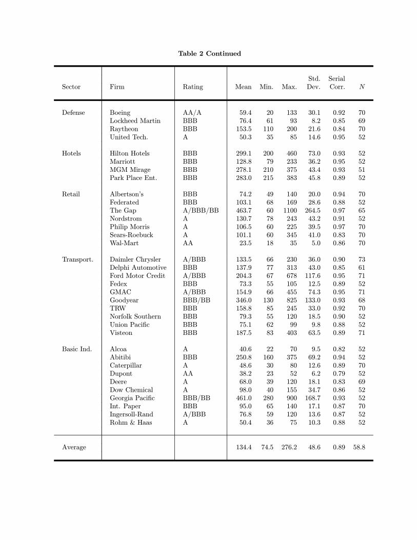
Table 2 Continued

Std. SerialSector Firm Rating Mean Min. Max. Dev. Corr. N

Defense Boeing AA/A 59.4 20 133 30.1 0.92 70Lockheed Martin BBB 76.4 61 93 8.2 0.85 69Raytheon BBB 153.5 110 200 21.6 0.84 70United Tech. A 50.3 35 85 14.6 0.95 52

Hotels Hilton Hotels BBB 299.1 200 460 73.0 0.93 52Marriott BBB 128.8 79 233 36.2 0.95 52MGM Mirage BBB 278.1 210 375 43.4 0.93 51Park Place Ent. BBB 283.0 215 383 45.8 0.89 52

Retail Albertson’s BBB 74.2 49 140 20.0 0.94 70Federated BBB 103.1 68 169 28.6 0.88 52The Gap A/BBB/BB 463.7 60 1100 264.5 0.97 65Nordstrom A 130.7 78 243 43.2 0.91 52Philip Morris A 106.5 60 225 39.5 0.97 70Sears-Roebuck A 101.1 60 345 41.0 0.83 70Wal-Mart AA 23.5 18 35 5.0 0.86 70

Transport. Daimler Chrysler A/BBB 133.5 66 230 36.0 0.90 73Delphi Automotive BBB 137.9 77 313 43.0 0.85 61Ford Motor Credit A/BBB 204.3 67 678 117.6 0.95 71Fedex BBB 73.3 55 105 12.5 0.89 52GMAC A/BBB 154.9 66 455 74.3 0.95 71Goodyear BBB/BB 346.0 130 825 133.0 0.93 68TRW BBB 158.8 85 245 33.0 0.92 70Norfolk Southern BBB 79.3 55 120 18.5 0.90 52Union Pacific BBB 75.1 62 99 9.8 0.88 52Visteon BBB 187.5 83 403 63.5 0.89 71

Basic Ind. Alcoa A 40.6 22 70 9.5 0.82 52Abitibi BBB 250.8 160 375 69.2 0.94 52Caterpillar A 48.6 30 80 12.6 0.89 70Dupont AA 38.2 23 52 6.2 0.79 52Deere A 68.0 39 120 18.1 0.83 69Dow Chemical A 98.0 40 155 34.7 0.86 52Georgia Pacific BBB/BB 461.0 280 900 168.7 0.93 52Int. Paper BBB 95.0 65 140 17.1 0.87 70Ingersoll-Rand A/BBB 76.8 59 120 13.6 0.87 52Rohm & Haas A 50.4 36 75 10.3 0.88 52

Average 134.4 74.5 276.2 48.6 0.89 58.8

Table 3

Estimation Results from Fitting the Credit Model to the Corporate Bonds. This table presentsparameter estimates and summary statistics from fitting the credit model to the bonds of the indicatedfirms. The mean λ reported is the time series average of the estimated intensity process. The number ofbonds represents the number of bonds used in estimating the parameters of the model. RMSE denotesthe root-mean-squared error across all bonds and observation dates used in the estimation. The averagesreported at the bottom of the table are cross-sectional averages of the indicated parameters and summarystatistics taken over all firms. The risk-neutral dynamic model for the intensity process is

dλ = (α − β λ) dt + σ√λ dZ.

NumberSector Firm α β σ Mean λ of Bonds RMSE

Financial AON 0.0030 0.0000 0.0105 0.0357 4 11.7Bank of America 0.0084 0.1292 0.0631 0.0069 6 12.0Bear Stearns 0.0189 0.4764 0.0423 0.0190 7 12.0Citigroup 0.0063 0.1242 0.0743 0.0112 6 9.5Countrywide Cr. 0.0127 0.1627 0.3305 0.0145 6 11.0CIT Group 0.0179 0.0000 0.7081 0.0557 4 23.5Capital One 0.1045 1.6596 1.3817 0.3229 5 54.7GE Capital 0.0086 0.2489 0.0984 0.0059 12 14.0Goldman Sachs 0.0145 0.2343 0.2168 0.0090 11 9.0Household Fin. 0.0130 0.2729 0.0099 0.0356 6 21.0JP Morgan Chase 0.0167 0.3710 0.1971 0.0081 15 17.0MBNA 0.0127 0.0000 0.0145 0.0200 5 19.6Lehman Brothers 0.0163 0.1387 0.4850 0.0118 7 10.0Merrill Lynch 0.0125 0.1877 0.3086 0.0098 18 13.7Morgan Stanley 0.0141 0.2938 0.0899 0.0084 9 12.1Bank One 0.0129 0.3291 0.0373 0.0068 8 13.2

Technology Walt Disney 0.0136 0.3091 0.2010 0.0156 7 17.5Sprint 0.0202 0.1981 0.3780 0.0223 9 15.8Hewlett Packard 0.0127 0.3475 0.1032 0.0303 4 10.7IBM 0.0128 0.5711 0.1073 0.0102 11 14.2Motorola 0.0164 0.2144 0.0801 0.0678 5 33.0Qwest Capital 0.0410 0.0000 1.3129 0.0632 7 18.0SBC 0.0132 0.3221 0.3604 0.0090 13 19.8Sun Microsystems 0.0054 0.0000 0.0193 0.0378 3 23.4AT&T 0.0052 0.0000 0.0003 0.0532 6 31.9Viacom 0.0150 0.0000 0.6358 0.0137 6 15.3Worldcom 0.0158 0.2353 0.0787 0.0333 11 15.1

Energy Amerada Hess 0.0028 0.0032 0.0340 0.0228 3 7.8Conoco 0.0045 0.0413 0.0455 0.0155 5 9.6Duke Capital 0.0261 0.0004 1.0999 0.0408 5 24.7Con Edison 0.0134 0.3139 0.0016 0.0097 4 11.1Enron 0.0054 0.0534 0.0422 0.0295 8 7.1Occidental 0.0187 0.6652 0.1170 0.0372 5 16.1

Table 3 Continued

NumberSector Firm α β σ Mean λ of Bonds RMSE

Defense Boeing 0.0110 0.3023 0.1005 0.0163 8 14.5Lockheed Martin 0.0165 0.5640 0.2226 0.0231 4 11.8Raytheon 0.0080 0.0721 0.2773 0.0320 10 13.8United Tech. 0.0141 0.2755 0.4709 0.0053 5 11.8

Hotels Hilton Hotels 0.0184 0.0109 0.3230 0.0511 4 15.5Marriott 0.0159 0.1382 0.3368 0.0351 4 19.6MGM Mirage 0.0176 0.0543 0.3491 0.0648 7 22.0Park Place Ent. 0.0000 0.0198 0.1456 0.0867 7 26.4

Retail Albertson’s 0.0194 0.5179 0.1491 0.0253 4 12.8Federated 0.0025 0.0004 0.0047 0.0283 4 21.3The Gap 0.0118 0.0003 0.1993 0.0821 7 42.8Nordstrom 0.0165 0.0871 0.0018 0.0172 3 11.2Philip Morris 0.0142 0.3096 0.0467 0.0191 7 12.7Sears-Roebuck 0.0139 0.2809 0.0021 0.0240 9 17.5Wal-Mart 0.0089 0.3511 0.0481 0.0033 9 10.4

Transport. Daimler Chrysler 0.0063 0.0584 0.0950 0.0301 6 9.8Delphi Automotive 0.0003 0.0018 0.0064 0.0427 3 18.7Ford Motor Credit 0.0122 0.2151 0.0230 0.0466 7 16.8Fedex 0.0133 0.0784 0.4815 0.0258 5 11.2GMAC 0.0042 0.0085 0.0206 0.0328 10 13.5Goodyear 0.0132 0.0277 0.5808 0.1320 4 14.7TRW 0.0013 0.0009 0.0460 0.0445 7 16.1Norfolk Southern 0.0194 0.5852 0.1171 0.0180 6 12.2Union Pacific 0.0000 0.0000 0.2072 0.0299 8 12.0Visteon 0.0032 0.0004 0.0130 0.0437 2 9.6

Basic Ind. Alcoa 0.0131 0.4064 0.2180 0.0107 3 10.6Abitibi 0.0015 0.0014 0.0082 0.0588 4 10.4Caterpillar 0.0129 0.0103 0.3603 0.0042 2 10.0Dupont 0.0119 0.5364 0.1901 0.0028 5 8.9Deere 0.0143 0.3307 0.2282 0.0177 7 9.0Dow Chemical 0.0126 0.1464 0.4127 0.0223 5 14.4Georgia Pacific 0.0139 0.4850 0.1588 0.1992 4 41.6Int. Paper 0.0152 0.2143 0.4262 0.0249 7 6.9Ingersoll-Rand 0.0085 0.0048 0.0212 0.0148 5 9.8Rohm&Haas 0.0058 0.0089 0.2682 0.0151 2 5.0

Average 0.0133 0.2060 0.0303 0.0356 6.4 15.9

Table 4

Summary Statistics for the Differences Between Model Implied and Market Credit-DefaultSwap Premia. This table reports summary statistics for the differences between the premia implied bythe fitted credit model and market premia for the indicated firms. Differences are expressed in basis points.Averages reported at the bottom of the table are cross-sectional averages of the indicated summary statisticstaken over all firms.

Average SerialSector Firm Difference t-Statistic Min. Max. Corr.

Financial AON 71.5 5.2 −254.7 171.8 0.83Bank of America 67.3 31.4 35.2 104.0 0.91Bear Stearns 81.0 64.0 55.2 107.0 0.65Citigroup 61.4 37.6 28.9 90.2 0.83Countrywide Cr. 54.4 18.8 −18.9 88.8 0.57CIT Group 19.6 2.3 −220.3 93.1 0.41Capital One 31.8 2.0 −567.0 153.3 0.37GE Capital 40.1 15.7 −3.4 98.7 0.90Goldman Sachs 79.6 49.7 45.6 111.1 0.85Household Fin. 31.1 5.9 −93.2 89.3 0.66JP Morgan Chase 76.6 48.6 40.4 102.1 0.74MBNA 73.6 15.2 −23.3 122.4 0.67Lehman Brothers 73.2 45.8 41.0 103.7 0.81Merrill Lynch 59.1 30.6 25.5 87.9 0.87Morgan Stanley 75.0 58.5 45.5 97.2 0.80Bank One 68.6 45.4 49.6 92.6 0.82

Technology Walt Disney 56.9 19.1 −27.8 88.5 0.86Sprint 65.8 9.4 −147.8 96.6 0.64Hewlett Packard 52.2 21.3 13.4 90.3 0.69IBM 34.5 11.0 −11.5 102.5 0.96Motorola 58.4 8.5 −82.1 184.5 0.70Qwest Capital 19.1 2.7 −28.2 56.0 0.43SBC 25.5 4.6 −125.5 92.7 0.81Sun Microsystems 62.5 5.9 −92.9 173.9 0.95AT&T 51.5 7.6 −117.0 183.0 0.74Viacom 68.1 36.9 30.2 94.5 0.80Worldcom 65.8 24.9 24.5 90.7 0.71

Energy Amerada Hess 63.4 39.6 40.8 93.1 0.81Conoco 52.6 21.7 31.8 109.3 0.89Duke Capital 32.6 3.0 −349.5 100.4 0.47Con Edison 78.2 27.9 36.5 111.1 0.89Enron 12.5 1.8 −136.3 63.1 0.58Occidental 73.2 34.8 43.4 111.9 0.77

Table 4 Continued

Average SerialSector Firm Difference t-Statistic Min. Max. Corr.

Defense Boeing 66.5 33.7 −6.4 97.2 0.58Lockheed Martin 52.6 54.2 31.3 71.2 0.67Raytheon 30.0 10.1 −16.1 88.7 0.83United Tech. 53.0 36.6 27.8 74.5 0.80

Hotels Hilton Hotels 60.2 9.4 −145.3 141.2 0.56Marriott 101.4 18.9 −11.9 159.4 0.92MGM Mirage 88.5 16.1 16.2 193.9 0.86Park Place Ent. 99.5 17.1 31.6 206.9 0.85

Retail Albertson’s 85.4 50.1 44.6 111.5 0.87Federated 66.0 21.5 0.3 97.6 0.77The Gap 17.2 1.4 −327.3 196.9 0.77Nordstrom 106.0 23.1 28.4 155.0 0.87Philip Morris 49.9 12.6 −44.1 102.4 0.94Sears-Roebuck 73.6 18.0 −137.3 117.5 0.74Wal-Mart 48.7 39.5 29.4 69.4 0.91

Transport. Daimler Chrysler 58.8 25.6 −1.4 98.8 0.77Delphi Automotive 75.7 18.2 −79.3 126.9 0.68Ford Motor Credit 44.5 8.9 −187.0 114.4 0.45Fedex 98.2 94.3 82.2 113.2 0.53GMAC 51.7 15.0 −89.3 87.8 0.64Goodyear 84.1 10.5 −140.9 323.7 0.54TRW 74.3 29.8 27.6 134.6 0.73Norfolk Southern 57.6 25.6 28.3 124.2 0.82Union Pacific 52.5 29.6 24.0 83.2 0.78Visteon 65.6 14.2 −99.3 139.4 0.69

Basic Ind. Alcoa 66.4 38.2 32.1 94.9 0.77Abitibi 56.4 10.2 −22.2 141.8 0.76Caterpillar 87.5 65.9 58.3 114.4 0.83Dupont 35.3 20.0 16.7 70.8 0.94Deere 73.5 52.5 28.2 91.9 0.68Dow Chemical 56.5 16.7 −32.3 93.3 0.65Georgia Pacific 26.7 2.0 −295.2 263.2 0.49Int. Paper 70.8 35.6 34.4 109.5 0.83Ingersoll-Rand 93.7 39.7 49.6 133.6 0.75Rohm&Haas 67.6 30.9 43.6 106.2 0.93

Average 60.8 25.0 −39.9 117.7 0.74

Table 5

Regression of Pricing Differences on Tax and Liquidity Proxies. This table reports the results fromregressing the pricing differences between the implied and market credit-default swap premia on the averagecoupon rate of the bonds, the average bid-ask spread of the bonds, the volatility of changes in the averageyield spreads of the bonds, and the number of bonds in the bracketing set, as well as on the on-the-run/off-the-run Treasury spread and the Agency-Treasury or flight-to-liquidity spread. The t-statistics are based onthe Newey-West estimate of the covariance matrix.

Difference = β0 + β1 Coupon

+ β2 Bid/Ask Spread

+ β3 Vol of Spread

+ β4 Number of Bonds

+ β5 On/Off the Run Spread

+ β6 Agency Spread +

Variable β Coefficient t-Statistic

Intercept −10.085 −1.04Coupon 9.878 6.92

Bid/Ask Spread 0.425 2.45Vol of Spread −0.742 −6.12

Number of Bonds −1.005 −3.35On/Off the Run Spread 0.996 2.08

Agency Spread 0.590 2.89

R2 0.098

N 3670

Table 6

Summary Statistics from Robustness Checks. The columns labeled constant coupon present summarystatistics for the differences between the constant-coupon spreads and the market premia for the indicatedfirms. The columns labeled swap curve present summary statistics for the differences between the impliedand market premia when the swap curve is used to generate the discount curve. The last column reportsthe implied probability of a counterparty default required to account for the average differences reported inTable 4. Averages reported at the bottom of the table are cross-sectional averages of the indicated summarystatistics taken over all firms.

Constant Coupon Swap CurveImplied

Sector Firm Ave. Diff. t-stat. Ave. Diff. t-stat. Prob.

Financial AON 72.2 5.2 11.9 0.9 33.8Bank of America 72.3 26.7 9.7 7.0 63.2Bear Stearns 89.0 56.9 22.9 16.7 52.3Citigroup 66.0 33.1 1.7 1.3 60.1Countrywide Cr. 53.7 16.9 1.2 0.4 38.1CIT Group 30.9 3.9 −33.6 −4.1 8.1Capital One 107.2 6.6 −27.3 −1.7 7.7GE Capital 46.8 16.0 −17.5 −9.5 46.2Goldman Sachs 93.5 47.2 18.1 13.2 57.0Household Fin. 40.6 8.3 −21.9 −4.7 15.4JP Morgan Chase 83.0 43.9 18.2 12.2 58.3MBNA 69.5 14.1 21.3 4.3 30.0Lehman Brothers 75.1 34.8 15.1 12.0 49.3Merrill Lynch 59.8 25.9 −1.1 −0.7 47.0Morgan Stanley 73.1 40.2 14.5 11.6 57.5Bank One 76.7 38.4 14.0 11.1 60.7

Technology Walt Disney 52.7 18.1 −8.0 −3.1 41.4Sprint 68.4 9.7 −3.2 −0.5 32.0Hewlett Packard 58.4 22.3 −3.1 −1.3 31.9IBM 37.6 12.3 −22.9 −10.5 38.6Motorola 57.6 9.0 9.4 1.3 16.8Qwest Capital 27.1 3.8 −40.7 −5.8 7.4SBC 23.9 4.4 −27.9 −5.6 23.8Sun Microsystems 70.0 6.6 12.2 1.2 25.1AT&T 50.1 7.5 −6.3 −1.0 16.0Viacom 69.7 42.4 6.7 4.6 47.6Worldcom 68.9 24.9 −7.8 −2.3 28.9

Energy Amerada Hess 68.0 37.4 13.2 9.0 43.9Conoco 54.8 19.9 2.8 1.4 44.2Duke Capital 56.2 5.3 −17.8 −1.7 16.9Con Edison 87.1 29.0 23.9 8.8 61.9Enron 15.7 2.3 −61.1 −9.6 6.7Occidental 86.3 34.0 23.5 13.3 48.3

Table 6 Continued

Constant-Coupon Swap Curve

ImpliedSector Firm Ave. Diff. t-stat. Ave. Diff. t-stat. Prob.

Defense Boeing 68.5 30.3 9.5 4.5 52.8Lockheed Martin 60.7 48.1 −2.1 −1.8 40.8Raytheon 35.8 11.4 −29.3 −14.7 16.3United Tech. 57.0 41.0 −2.1 −1.0 51.3

Hotels Hilton Hotels 73.2 11.7 10.0 1.5 16.8Marriott 105.1 18.7 41.4 8.2 44.1MGM Mirage 96.6 18.2 35.5 6.7 24.1Park Place Ent. 116.2 19.5 40.0 7.4 26.0

Retail Albertson’s 92.1 44.9 27.3 18.5 53.5Federated 80.0 28.8 23.6 7.1 39.0The Gap −3.3 −0.3 −40.9 −3.3 3.6Nordstrom 109.5 22.7 51.6 10.9 44.8Philip Morris 49.6 11.6 −7.8 −2.3 31.9Sears-Roebuck 76.3 18.6 15.1 4.0 42.1Wal-Mart 42.1 22.8 −17.6 −15.8 67.4

Transport. Daimler Chrysler 62.6 23.5 0.2 0.1 30.6Delphi Automotive 83.8 21.0 23.0 5.1 35.4Ford Motor Credit 55.5 11.8 −20.1 −3.3 17.9Fedex 103.5 70.4 43.1 40.4 57.3GMAC 55.8 15.4 −6.1 −2.1 25.0Goodyear 94.1 12.8 24.9 3.2 19.6TRW 85.3 33.7 16.7 7.9 31.9Norfolk Southern 67.8 28.0 4.1 1.6 42.1Union Pacific 63.5 37.8 −1.7 −1.2 41.2Visteon 86.8 18.2 11.3 2.4 25.9

Basic Ind. Alcoa 71.1 33.4 10.8 7.1 62.1Abitibi 69.8 12.6 9.1 1.9 18.4Caterpillar 67.1 30.9 21.5 14.1 64.3Dupont 31.5 13.2 −22.1 −10.8 48.0Deere 76.4 49.5 16.8 9.7 51.9Dow Chemical 60.7 16.8 5.1 1.5 36.6Georgia Pacific 34.9 3.1 −28.4 −2.2 5.5Int. Paper 80.6 33.3 15.4 10.7 42.7Ingersoll-Rand 58.4 22.3 25.9 12.6 54.9Rohm&Haas 69.3 26.3 20.7 17.4 57.3

Average 66.2 23.1 3.9 3.2 37.3

Table7

Summary

ofResultsfromtheEstimationoftheVectorAutoregressionModel.Thistablereportsthenumberoffirmsforwhichthe

indicatedvariableshavesignificantforecastingpower.Thetotalnumberoffirmsforwhichthemodelisestimatedis67.Whenthelaglengthkisone,

significanceisbasedonthet-statisticsofindividualcoefficients.Whenthelaglengthkistwo,significanceisbasedonaWaldtestforthesignificance

ofcoefficientsjointly.ThesignificanceoftheoverallregressionisbasedonastandardFtest.

∆St=a1+

k

j=1

b 1j∆St−j+

k

j=1

c 1j∆Ct−j+

k

j=1

d1jRt−j+

1,

∆Ct=a2+

k

j=1

b 2j∆St−j+

k

j=1

c 2j∆Ct−j+

k

j=1

d2jRt−j+

2,

Rt=a3+

k

j=1

b 3j∆St−j+

k

j=1

c 3j∆Ct−j+

k

j=1

d3jRt−j+

3,

LaggedExplanatoryVariable

Forecasting

LagLength

Equation

Premium

BondSpread

StockReturn

Overall

1Premium

1213

1714

BondSpread

235

1430

StockReturn

125

38

2Premium

1012

1212

BondSpread

214

2137

StockReturn

105

37

1/1/01 4/1/01 7/1/01 10/1/010.02

0.025

0.03

0.035

0.04

0.045

0.05

0.055

0.06

9/5/01

10/16/01

10/22/01

Impl

ied

Def

ault

Inte

nsity

Date

Fig. 1. Enron’s implied default intensity. This figure shows the defaultintensity implied from Enron corporate bond yields between December 5,2000 and October 22, 2001. The arrows indicate the dates of importantcorporate events enumerated in Table 1.

100

200

300

400

500

9/5/01

10/16/01

10/22/01

Bas

is P

oint

sMarket PremiumImplied Premium

1/1/01 4/1/01 7/1/01 10/1/01 1/1/020

50

1009/5/01

10/16/01

10/22/01

12/2/01

Sto

ck P

rice

Date

Fig. 2. Enron’s market credit-default swap premium, implied credit-defaultswap premium, and stock price. The top plot shows Enron’s market and im-plied credit-default swap premia between December 5, 2000 and October 22,2001. The bottom plot shows Enron’s stock price between December 5, 2000and December 7, 2001. The arrows on each plot indicate the dates of impor-tant corporate events enumerated in Table 1. Enron filed for bankruptcy onDecember 2, 2001.

10 20 30 40 50 60 70 80 90 100 1100

1

2

3

4

5

6

7

8

9

10

Average Difference (Basis Points)

Fre

quen

cy

Fig. 3. Distribution of the average difference between the implied and mar-ket credit-default swap premia. For each firm in the sample, the averagedifference is calculated as the time-series average of the difference betweenthe implied credit-default swap premium and the market credit-default swappremium. The plot shows the cross-sectional distribution of the averagedifference for the 68 firms in the sample. The cross-sectional mean of theaverage difference is 60.8 basis points. The standard deviation of the averagedifference is 21.2 basis points.