U.S. Inequality and Fiscal Progressivity -- An Intragenerational Accounting

Alan J. Auerbach

University of California, Berkeley

Laurence J. Kotlikoff Boston University and The Fiscal Analysis Center

Darryl Koehler

Economic Security Planning, Inc. and The Fiscal Analysis Center

April 13, 2016, Revised August 29, 2019

We thank the National Center for Policy Analysis, the Searle Family Trust, the Sloan Foundation, the Goodman Institute, the Robert D. Burch Center for Tax Policy and Public Finance at the University of California, Berkeley, and Boston University for research support. We also thank Emmanuel Saez, other participants in the October 2015 Boskin Fest at Stanford, participants in the June, 2019 Journées Louis-André Gérard-Varet in Aix-en-Provence, and four anonymous referees for very helpful comments.

Abstract

This study measures inequality and fiscal progressivity. It differs from prior such analyses by measuring inequality based on remaining lifetime spending rather than particular resources, like wealth and current income, that only partially determine lifetime spending, and by considering inequality and progressivity within generations. To estimate the distribution of remaining lifetime spending, we run the 2016 Federal Reserve Survey of Consumer Finances (after imputing missing data from other surveys) through The Fiscal Analyzer (TFA), a life-cycle consumption-smoothing program that incorporates remaining life-time resources, borrowing constraints and all major federal and state tax and transfer programs. We find that inequality in wealth and income dramatically overstate inequality in remaining lifetime spending. For example, the richest 1 percent of forty year olds, where resources are measured as the sum of human plus non-human wealth, have 34.1 percent of the cohort’s total non-human wealth, but account for only 14.5 percent of the cohort’s total remaining lifetime spending. The poorest quintile of forty year olds own just 0.6 percent of the cohort’s wealth, but account for 7.3 percent of its remaining lifetime spending. We also find that within-cohort inequality differs considerably from inequality across the entire population, regardless of age, and that, for particular age cohorts, current-year net tax rates substantially understate the degree of progressivity. Finally, as we illustrate by for the 2017 Tax Cuts and Jobs Act, the progressivity of tax reform may be significantly misstated using conventional current-year analysis. .

I. Introduction

Inequality is a topic of intense national and international interest thanks to the growing

dispersion of income and wealth around the world and particularly in the United States.

Piketty, Saez, and Zucman (2018) report that average real income of the top 10 percent of

income-ranked U.S. households grew by 113 percent between 1984 and 2014, while the real

income of the top 0.1 percent grew by 298 percent. By contrast, the average real income of

the lowest 50 percent grew by 21 percent. While the trend in wealth shares is more difficult

to estimate precisely because of the need to impute values of unobserved wealth

components, there is little doubt about the direction of wealth inequality. For example, from

1989 through 2013, the Congressional Budget Office (2016) estimates that wealth of families

in the top 10 percent of the wealth distribution rose by 54 percent, whereas median wealth

rose by only 4 percent. By 2013, the 50 percent poorest Americans, ranked on the basis of

their wealth, owned a mere 1 percent of total net wealth. 1 Indeed, the richest three

Americans – Jeff Bezos, Bill Gates, and Warren Buffett – collectively own more wealth than

the poorest 50 percent of Americans, who number 160 million!2

As documented by Kopczuk, Saez, and Song (2010), wage inequality, while less

pronounced than income or wealth inequality, is also significant and growing. Studies by

Goldin and Katz (2008) and Acemoglu and Autor (2011) show a steady and dramatic 75

1 Note that this ranks all households by wealth rather than remaining lifetime resources, the ranking method we use below. In our 2016 SCF data, the poorest 40 percent of households ages 20 to 79, ranked in terms of lifetime resources, account for almost 10 percent of total net wealth. 2 https://www.forbes.com/sites/noahkirsch/2017/11/09/the-3-richest-americans-hold-more-wealth-than-bottom-50-of-country-study-finds/#330015943cf8

2

percent increase in the college/high school wage premium over the last three decades, with

typical college graduates now earning twice the wage of high school graduates.3

These studies are important and interesting but, for understanding inequality they all

fall short. None measures inequality in remaining lifetime spending (RLS), which is arguably

the ultimate concern when assessing economic fairness.4 The shortcomings are two-fold.

First, a sufficiently progressive fiscal system can transform the most unequal distribution of

market resources into a more equal distribution of resources available for consumption.

Second, individual components of current resources, whether wealth or current income,

provide an inadequate measure of a household’s overall capacity to finance consumption.

Such components ignore both future labor income as well as future taxes and transfer

payments, the importance of which varies systematically by age.

This study uses a life-cycle, consumption-smoothing program, called The Fiscal

Analyzer (TFA), to infer remaining lifetime spending among respondents to the 2016 Federal

Reserve Survey of Consumer Finances. TFA does life-cycle consumption-smoothing across

all possible survivor paths taking into account survivor-path specific labor earnings,

borrowing constraints, federal and state taxes, and federal and state transfer payments. Our

goal is measuring remaining lifetime spending inequality controlling for preference

differences and responses to the fiscal system. Our assumption of uniform (across

households) Leontief consumption preferences with age-specific time-preference factors

(assumed identical in our base case calculations) as well as exogenous labor supply achieves

3 See, in particular, Figure 1 in Acemoglu and Autor (2011). 4 By RLS we mean the present value of a household’s remaining expected future lifetime expenditures, including imputed rent on owned homes and the household’s expected future bequests, where “expected” references averaging over the realized present value of annual spending along each potential household survival path. We describe this measure further below.

3

this objective. Assuming that preferences are identical across households controls for

preference differences; and the assumption of Leontief intertemporal consumption

preferences and exogenous labor supply ensures no substitution of consumption or leisure

today for consumption or leisure tomorrow in response to the fiscal system.

TFA smooths consumption over time, but also over survivor states by determining

annual life insurance amounts that decedents in year t, were they to die in that year, need to

leave survivors to ensure survivors can afford, to the dollar, the same future living standard

as they would enjoy absent the decedent’s death. Life insurance purchases are assumed to

be non-negative, i.e., households don’t buy annuities at the margin.

As described below, the TFA does its consumption smoothing over time and survivor

states in one integrated, iterative process, which simultaneously determines the household’s

paths of net taxes under each survivor path. Once it has generated its survivor path-specific

results, TFA determines each household’s actuarial expected (average across survivor paths)

present value of future spending, including bequests. The difference between expected

remaining lifetime spending and expected remaining lifetime resources is the household’s

expected remaining lifetime net tax payment. The ratio of remaining lifetime net tax

payments to remaining lifetime resources provides our measure of lifetime average net tax

rates. We measure fiscal progressivity within cohort by considering how these average

remaining lifetime net tax rates rise with remaining lifetime resources.5

5 Our calculation of average net tax rates is resource-weighted. That is, rather than simply forming the ratio T/R for each household within a cohort-specific resource percentile range and then applying SCF population weights, we instead apply resource weights. This places smaller weight on outlier households that have exceptionally large or small net tax rates, but who represent a relatively small share of the resource distribution.

4

A. The Remaining Lifetime Spending (RLS) Perspective

There are several reasons to take a lifetime- rather than a current-year (based on current-

year wealth or income) perspective in assessing inequality and fiscal progressivity, and to

do so separately for different age cohorts. First, the patterns of income, taxes, and transfer

payments differ significantly and systematically over the life cycle. A current-year

perspective may provide a distorted view of a household’s lifetime spending capacity as well

as the progressivity of the fiscal system. Second, annual variations in income, particularly

due to the realization of capital gains, mean that annual income may be a very imperfect

indicator of longer-run spending capacity. Finally, households at different ages, at different

stages of the life cycle, have incomes, taxes, and transfer payments that relate quite

differently to longer-run spending capacity. For example, a retiree who is a year from

collecting their Social Security benefits and starting his or her retirement account

withdrawals may have far higher income in future years.

Unfortunately, there are no longitudinal data that report RLS. There are data on

current-year consumption (see, e.g., Meyer and Sullivan, 2017). But, even with consumption

smoothing, current consumption may be an inadequate indicator of remaining lifetime

spending. Borrowing constraints, which our analysis suggests affect the majority of SCF

respondents, may depress current consumption relative to future consumption. Households

also leave bequests, which we treat as a form of consumption spending. Here, too, current

consumption can materially differ from future consumption.

Our methodology is based on a) estimated lifetime resources – the household’s

current net wealth and its current and projected future labor earnings; b) the taxes we

estimate it will pay and transfer payments it will receive along all survival paths; and c)

5

assumed uniform life-cycle consumption-smoothing behavior subject to borrowing

constraints. We use this method to assess both U.S. RLS inequality and fiscal progressivity.

Notwithstanding our assumed preference for full consumption smoothing, the longitudinal

age-consumption (age-living standard per equivalent adult) profiles of our SCF households

differ dramatically due to differences in their timing and frequency of borrowing constraints.

One might quickly object that consumption growth rates vary by household due, not

just, as mentioned, differences in intertemporal preferences, but also risk.6 We plan, in

future work, to explore the interplay between resource inequality, preferences, risk, and

government policy. But a first step in that process – the one taken here -- is examining

spending inequality and fiscal progressivity controlling for differences in intertemporal

preferences (and, for that matter, labor-leisure preferences).

To form our measures of RLS and fiscal progressivity, we run the 2016 Federal

Reserve Survey of Consumer Finances (SCF) sample through The Fiscal Analyzer (TFA).7

As described briefly below and in detail in our online appendix, TFA does iterative

dynamic program. Specifically, it iterates to convergence across three programs – a

consumption smoothing program, a life insurance program, and a net tax program. Each

program passes its results to the other two programs, which take those results as inputs.

6 Risks may also differ across households. This question, too is reserved for future research. Differences in intertemporal consumption preferences may reflect behavioral factors identified by Laibson (1997) and others. While we assume uniform retirement ages, our earnings projections are predicated on reported earnings, which reflect a combination of labor supply choice and wage rates. 7 This project initially relied on the 2013 SCF, switching to the 2016 SCF when it became available. The results from the 2013 SCF are remarkably similar to those reported here.

6

B. Household Remaining Lifetime Budget Constraints

Along any realized survival path, i, a household’s realized present value of remaining lifetime

spending, discretionary plus non-discretionary, is denoted Si. The household’s

intertemporal budget requires

(1) 𝑆𝑆𝑖𝑖 = 𝑅𝑅𝑖𝑖 − 𝑇𝑇𝑖𝑖,

where Ri and Ti reference, respectively, the realized present values of the household’s

remaining lifetime resources and remaining lifetime net taxes along survival path i. The

realized present value of remaining lifetime resources, Ri, is the sum of the household’s

current net wealth, W, and the realized present value of its future labor earnings, Hi. I.e.,

(2) 𝑅𝑅𝑖𝑖 = 𝑊𝑊 + 𝐻𝐻𝑖𝑖.

The expected present value of remaining lifetime spending, S, resources, R, and net taxes, T,

satisfy

(3) S = ∑ 𝑝𝑝𝑖𝑖𝑆𝑆𝑖𝑖𝑖𝑖 ,

(4) H = ∑ 𝑝𝑝𝑖𝑖𝐻𝐻𝑖𝑖𝑖𝑖 ,

(5) T = ∑ 𝑝𝑝𝑖𝑖𝑇𝑇𝑖𝑖𝑖𝑖 ,

and

(6) R = ∑ 𝑝𝑝𝑖𝑖𝑅𝑅𝑖𝑖𝑖𝑖 ,

where pi is the probability the household experiences survival path i. The above equations

imply

(7) 𝑅𝑅 = 𝑊𝑊 + 𝐻𝐻

and

(8) 𝑆𝑆 = 𝑅𝑅 − 𝑇𝑇.

7

Again, while inequality in R and its two components, W and H, may be of independent

interest and have been the subject of considerable recent research, our focus is on ultimate

inequality, i.e., inequality in S. We would certainly anticipate that S, like R, is extremely

unequally distributed in the United States. This said, a key policy question is the extent to

which progressivity in the distribution of T mitigates inequality in the distribution of S.

Our study measures inequality in S on a cohort-specific basis (i.e., intragenerational),

compares it with cohort-specific inequality in W and H, and determines the degree to which

cohort-specific inequality in T reduces cohort-specific inequality in S.8 We also show that

fiscal progressivity measured, within cohort, via the average remaining lifetime net tax rate,

τ, defined in equation (9), can differ markedly from the much more common measure of fiscal

progressivity made on a current-year basis and without regard to age.

(9) 𝜏𝜏 = 𝑇𝑇𝑅𝑅� .

The term “net taxes” references all major federal and state tax and transfer programs,

including the federal personal income tax, the FICA payroll tax, state income taxes, state sales

taxes, the federal corporate income tax, the federal and state estate taxes, state-specific TANF

welfare benefits, state-specific SNAP (Food Stamps) programs, Supplemental Security

Income, state-specific Obamacare (ACA) healthcare subsidies, Social Security retirement

benefits, Social Security auxiliary benefits, Social Security disability benefits, state-specific

8 In doing so, we do not consider the extent to which changes in government policy through T have general equilibrium effects on the elements of R, as will be the case if government tax and transfer programs influence decisions to work and save. Thus, our estimates of the impact of government policy on progressivity are of a partial equilibrium nature, taking the underlying distribution of resources as given.

8

Medicaid benefits, Medicare benefits, and Medicare Part B premiums. Details of TFA’s tax

and transfer calculations are provided here in the online appendix.9

C. Fiscal Labeling Issues

As we have emphasized repeatedly in our own work (e.g., Kotlikoff, 1984 and 1988,

Auerbach and Kotlikoff, 1987, Auerbach, Gokhale, and Kotlikoff, 1991, Kotlikoff, 2002, and

Green and Kotlikoff, 2006), while measures such as consumption are well-defined, others,

such as taxes and transfer payments, are not.10 Forward-looking measures such as those

considered here substantially lessen the problem; this was one of the important motivations

for our previous work developing generational accounting. For example, a change simply in

future labeling of social security transactions, from the taxes and transfers under a “public”

system to the purchase of government bonds and future debt service under a “private”

system, would have no impact on remaining lifetime spending, even though it would change

annual flows of taxes and transfers. Still, some types of government policy interventions

would affect our measures as well. For example, a policy equivalent to raising the minimum

wage could be constructed using government taxes on employment and transfers to

workers; our approach would not yield the same average tax rate calculations for these

equivalent policies, because we take market wages as given. Given the labeling problem, we

9 For example, in handling the federal personal income tax, it follows the 1040 form on a line-by-line basis taking into account the itemization decision, the Earned Income Tax Credit, the Child Tax Credit, the Alternative Minimum Tax, preferential capital gains and dividend taxation, the tax treatment of contributions to and withdrawals from 401(k), standard IRA, Roth, and other retirement accounts, the taxation of Social Security benefits, and Medicare’s high-income taxation of wages and asset income. For the Social Security benefit calculation, as another example, TFA includes the Early Retirement Benefit Reductions, the Delayed Retirement Credit, the Earnings Test, the Adjustment of the Reduction Factor, the Re-Computation of Benefits, and the system’s plethora of interconnected, across family members, benefit-eligibility conditions. 10 Different, but equally valid fiscal labeling conventions will change W and T by equal absolute amounts. Hence, as described below, average net tax rates depend on the specific conventions used.

9

need to be precise as to what our remaining lifetime net tax rates tell us. They tell us the

percentage reduction in the present value of remaining lifetime spending relative to the

lifetime spending that would arise were government taxes and transfer payments, as

currently labeled/defined by government, totally eliminated.

D. Preview of Findings

Our findings are striking. Under current law (including the provisions of the Tax Cuts and

Jobs Act of 2017, and assuming those provisions are permanent), the distribution of

remaining lifetime spending, while highly unequal, is considerably more equal than either

net wealth or current income. For example, the top 1 percent of 40-49 year olds ranked by

resources account for 34.1 percent of total cohort net wealth, but only 14.5 percent of total

cohort remaining lifetime spending. As for the lowest-resource quintile, it has just 0.6

percent of the cohort’s net wealth, but 7.3 percent of its total spending power.

Part of the explanation is that human wealth is more equally distributed than is net

wealth. The top 1 percent of this cohort account for 13.7 percent of the cohort’s human

wealth, which is roughly a third of its net wealth share. The bottom 20 percent have 4.9

percent of total-cohort human wealth – roughly eight times its net wealth share. The other

reason for lower spending than wealth inequality is the fiscal system. The average remaining

lifetime net tax rate of the top 1 percent of 40 year olds is 34.5 percent. It’s -46.6 percent

among those in the lowest quintile.

Which factor – greater equality in the distribution of human wealth or our

progressive fiscal system – makes the distribution of remaining lifetime spending so much

more equal than that of net wealth? The answer depends. With no fiscal system, the richest

1 percent of 40-49 year olds would account for 17.9 percent of RLS (their resource share),

10

which is far below their 34.1 percent of net wealth and close to their 14.5 percent of RLS. For

the poorest 20 percent, with just 0.6 percent of total cohort net wealth, their share of cohort

pre-fiscal resources is 4.0 percent.11 Hence, the more equal distribution of human wealth and

fiscal policy play a roughly equal role in raising the RLS share of the poorest quintile.

Our results are generally similar across cohorts. Within each cohort, those with the

lowest resources face significantly negative average remaining lifetime net tax rates, and

those with the highest resources face significantly positive average remaining lifetime net

tax rates. Consider, again, the cohort aged 40 to 49. Each dollar of remaining pre-tax lifetime

resources of those in the top 1 percent of the resource distribution is taxed, on average, at a

34.5 percent net rate. For those in the top quintile the average net tax rate is 28.4 percent.

But for those in the bottom quintile, every dollar of pre-tax resources is matched by a 46.6

percent net subsidy. Or, take those aged 60-69 in the top 1 percent of their cohort’s resource

distribution. Their remaining lifetime net tax rate is 20.6 percent. In contrast, those in the

lowest quintile face a negative average remaining net tax rate of -438.7 percent, reflecting

their proximity to receiving what for this group are vitally important Social Security,

Medicare, and Medicaid benefits.

Interestingly, longevity plays a relatively small role in determining fiscal

progressivity. Average net tax rates of those in the poorest quintile in each cohort would be

lower were they to live as long as those in the top quintile and, thereby, collect far more

benefits. Take the lowest quintile of 40-49 year olds and 60-69 year olds. These negative

11 This is slightly lower than their 4.9 percent share of human wealth

11

average net tax rates would fall to –48.1 percent and –495.0 percent from their respective

values of –46.6 percent and –438.7 percent.

E. Organization of Paper

The paper proceeds in Section II with a short literature review. Section III discusses TFA’s

methodology. Section IV presents our data and projections. Section V provides our main

results, first for the 40-49 year-old cohort and then, in less detail, for other cohorts. Section

VI provides an illustration of the model’s capacity to evaluate changes in tax policy, using the

2017 Tax Cuts and Jobs Act, and compares our findings to those based on traditional

approaches. Section VII discusses the sensitivity of our results to particular assumptions.

Finally, Section VIII concludes with a review of our key findings and their implications.

II. Prior Studies of Fiscal Progressivity

Since the classic work of Pechman and Okner (1974), the standard approach to calculating

the distributional effects of federal tax, or federal tax and transfer policy has been to classify

individuals or households by pre-tax income, possibly adjusting for family size, and then,

using particular assumptions about tax incidence (who bears the ultimate burden of any

particular tax), to assign taxes and transfers to different households. The Pechman-Okner

methodology has been retained, with refinements, notably in the continuing series of

analyses by the Congressional Budget Office (CBO; most recently in CBO, 2014). Such studies

generally find the U.S. fiscal system to be progressive, with the personal income tax (inclusive

of such elements as the Earned Income Tax Credit) playing an important role.

Economists have long suggested that current consumption, which is a proxy for

lifetime net of net-tax resources, rather than current income was more appropriate in

12

distinguishing the permanently rich from the permanently poor. Poterba (1989), for

example, compares the progressivity of excise taxes based on classifying households by

annual income with that based on classifying households by annual consumption. He shows

that the first approach makes excise taxes look much more regressive than the second.

Meyer and Sullivan (2017) find that the trend in increasing US inequality based on income,

even when accounting for taxes and transfers, is much less evident when one looks at

household consumption, not only because of consumption smoothing but also because of the

difficulties of measuring certain sources of income.

Fullerton and Rogers (1993) build on Poterba’s insight, considering the lifetime

incidence of tax systems more generally. Altig, et al. (2001) carry this approach further by

performing such analysis within a general equilibrium model with rational, forward-looking

households making lifetime planning decisions with respect to consumption and labor

supply. These studies, however, consider a subset of U.S. programs and model them in broad,

rather than fine detail.

Favreault, Smith, and Johnson (2015)’s major improvements to the Urban Institute’s

classic micro-simulation Dynasim Model provide a powerful tool for assessing the fiscal

system’s impact on households not just in the present, but through time. Their model grows

its sample demographically and stochastically, tracing likely socioeconomic and fiscal

impacts arising from predictable and unpredictable changes through time. Without

question, their framework has important advantages over ours in considering the interplay

between behavior and fiscal outcomes. This said, Dynasim’s behavioral assumptions, about

saving and labor supply, are ad hoc and, household specific. This makes the tool impractical

for achieving our goal, namely addressing inequality and the fiscal system holding constant

13

the reaction to the fiscal system. Dynasim drives its outcomes a forward basis, whereas with

borrowing constraints, one needs to do dynamic programming, i.e., work backwards. In

short, we have a different approach, which we judge far more straightforward to address the

questions we pose.

More recently, some analyses have considered the impacts of particular components

of the fiscal system on progressivity, attempting to incorporate the full range of program

details in their analysis. For example, Goda, Shoven, and Slavov (2011) estimate the

progressivity of the U.S. Social Security system within particular age cohorts, taking account

of how the program works as well as the projected mortality of individuals in different

lifetime income groups. Longevity is an important consideration, because Social Security is

an annuity-based transfer program, with lifetime payments dependent on longevity. This is

the type of analysis we perform here. But our actuarial analysis is of the entire U.S. fiscal

system, rather than of a particular component of the system. While studying individual fiscal

components is interesting in its own right, one cannot gain a picture of the fiscal system’s

overall effects from doing so.

A recent paper by Bengtsson, Holmlund, and Waldenstrom (2016) comes closest to

ours in focusing on lifetime fiscal progressivity and comparing lifetime with annual

progressivity. The authors use official Swedish data to track individuals over the years 1968

through 2009. Their methodology differs from ours in many respects. For example, we

incorporate all transfers, including healthcare transfers, we incorporate estate taxation, we

hold constant saving and labor supply behavior, and we examine the fiscal system at a point

in time, rather than looking at fiscal realizations as potentially modified by behavioral

responses and random outcomes. This is in line with our principal focus – understanding

14

whether current U.S. fiscal institutions are collectively progressive and assessing the degree

to which current-year average net tax rates approximate average remaining lifetime net tax

rates.12 Our approach also lets us evaluate the effects of actual or prospective changes in tax

and transfer polices on fiscal progressivity, as we do below for the recent Tax Cuts and Jobs

Act.

In their study, Bengtsson et al. (2016) show that progressivity is much smaller when

measured on a lifetime rather than a current-year basis. They attribute this, in part, to

mobility over time in one’s position in the income distribution. We view this as a very

important insight and one we intend to pursue in future research. In addition, they find that

transfer payments contribute significantly to the lower estimated lifetime progressivity.

Presumably, this is due to the fact that many important transfer payments, such as old-age

pensions and unemployment compensation, go to individuals whose current income is low

relative to their lifetime incomes. As we look separately at households in different age

cohorts, even our measures of progressivity based on current income will control for this

phenomenon to the extent that it is related to age (as in the case of old-age pensions).

III. TFA’s Algorithm

Rather than solve its deterministic problem in one program, TFA uses three dynamic

programs that iterate with one another, with each program taking the output of the other

two programs as given. The first program does consumption smoothing subject to borrowing

constraints, taking the time paths of life insurance premiums and net taxes as given. The

12 We intend to examine uncertainty in earnings and rates of return in future research. Of particular interest is assessing the extent to which the fiscal system insures against uncertainty in these variables.

15

second determines the life insurance needed by each spouse/partner at each date to ensure

survivors experience no decline in their living standard, where the living standard path is

determined in the first program. 13 The third program calculates, for each year, the

household’s payments to and receipts from each of the different tax and benefit programs it

faces.

The first program smooths the household’s consumption over the maximum survival

path – the path in which each spouse lives to his or her maximum age of life taking the time

path of net taxes and life insurance premiums on this maximum survival path as given. The

first routine’s goal is simple – maintain the household’s living standard per effective member

subject to a no-borrowing constraint. This form of consumption smoothing is consistent with

time-separable Leontief preferences. The second program determines how much life

insurance the household head and the potential spouse/partner need each year to ensure

the maintenance of survivors’ living standards (through their maximum ages of life and

through age 19, in the case of children) at annual levels at least as high as those that would

arise were no one to die prematurely.14 The output of this second program is the non-

negative life insurance premiums used by the first program. The third program calculates

the net taxes the household will pay along the survival path in which neither spouse dies

prematurely. It does so taking into account the path of total spending calculated in the first

program as well as the life insurance premiums calculated in the second program. In each

iteration, TFA updates its guesses about paths of spending, life insurance premium, and net

13 This routine calculates net taxes along each possible survivor path. 14 A reminder: The life insurance purchased at each date by the program for its household heads (and spouses, if married or partnered) is subject to non-negativity constraints. This second routine also calculates the net taxes and non-discretionary spending arising under each survivor path.

16

taxes using simple Gauss-Seidel weighting of old and new spending, insurance premiums,

and net tax paths.

Consumption-smoothing in our analysis is set to achieve a perfectly stable living

standard per household member subject, again, to the no-borrowing constraint. But, as

Appendix Figure 1 shows, the objective of complete smoothing subject to the no-borrowing

constraint leads to upward-sloping average age-consumption profiles. The figure shows, for

25 year-olds, 45 year-olds, and 65 year-olds, the average projected living standard under the

optimal path, conditional upon survival. 15 For 25 year olds, there is a considerable upward

slope until roughly age 40, indicating that borrowing constraints lead to spending that tracks

rising labor income. The growth of spending slows thereafter, but remains positive.16 For

65-year olds, there is a smooth, slowly rising average consumption profile.

IV. Data and Projections

As mentioned, our primary data come from the 2016 Survey of Consumer Finances (SCF) - a

cross-section survey that oversamples wealthy households in the process of collecting data

from some 6,500 American households. Our online appendix details sample selection,

15 Living standard is defined here as the household’s discretionary spending per adult with adjustments for economies in shared living and the relative cost of children. Discretionary spending references all spending apart from housing expenses and other off-the-top expenditures. The assumed relationship between discretionary spending, C, and living standard per equivalent adult, c, is given by C = c (N + .7K).6781, where N is the number of adults in the household and K the number of children. The constants .7 and .6781 reflect, respectively, our assumptions that children are 70 percent as expensive as adults and that two adults can live as cheaply together as 1.6 separately. 16 The large jumps at age 70 for 25 and 45 year olds reflect our assumption that individuals who indicate that they plan to work at least until age 70 or who express no plan to retire begin collecting Social Security benefits and begin making retirement account withdrawals at age 70, as is consistent with the maximum age for claiming Social Security benefits and for commencing retirement account withdrawals. Our online appendix discusses our procedures in more detail.

17

imputations and benchmarking of the 2016 SCF data. The survey includes data on assets,

liabilities, income, demographics, and a host of other socio-economic variables.

Running the TFA requires additional information not provided by the SCF. First, it

needs covered earnings histories to calculate future Social Security benefits. Second, it needs

state identifiers so that it can calculate state-specific taxes and transfer payments. As

described below, we use all past waves of the Current Population Survey (CPS) to impute

past Social Security covered earnings to our households as well as to project future covered

earnings.

Also, the public-use SCF release doesn’t provide state identifiers.17 Consequently, we

use the 2016 American Community Survey to allocate state-specific weights to each SCF

household such that the sum across states of each household’s weights equals the

household’s original SCF weight. Stated differently, we statistically matched the 2016 SCF

households with the U.S. Census’ 2016 American Community Survey. Our method assigned

each SCF household to each of the 51 states (including D.C.) in appropriate proportion such

that the sum of each household’s state-specific weight equals its original SCF weight.

A. Forecasting and Backcasting Labor Income

Our methodology requires, for each individual, a trajectory of labor earnings; past earnings

are needed to calculate Social Security covered earnings and future earnings are needed to

calculate the value of human wealth, H, a key component of remaining lifetime resources.

We use the CPS to statistically match SCF households for this purpose. In particular, we

17 The full SCF, available to Federal Reserve researchers, includes state identifiers, but they are not representative of a given state. I.e., one can’t use them to generate state-specific results.

18

define cells in each wave of the CPS by age, sex, and education18 and use successive waves to

estimate annual earnings growth rates by age and year for individuals in each sex and

education cell. These cell growth rates are used to “backcast” each individual’s earnings

history. We also project future earnings for each particular cell defined by age and

demographic group through age 67 (when we assume individuals claim retirement benefits)

by using average historical growth rates by age, net of average overall earnings growth and

plus an assumed future annual economy-wide average real wage growth rate of 1 percent.

These past and future growth rate estimates are for cell aggregates and do not

account for earnings heterogeneity within cells. To deal with such heterogeneity, we assume

that observed individual deviations in earnings from cell means are partially permanent and

partially transitory, based on an underlying earnings process in which the permanent

component (relative to group trend growth) evolves as a random walk and the transitory

component is serially uncorrelated. We also assume that such within-cell heterogeneity

begins in the first year of labor force participation.

In particular, suppose that, at each age, for group i, earnings for each individual j

evolve (relative to the change in the average for the group) according to a shock that includes

a permanent component, p, and an iid temporary component, e. Then, at age a (normalized

so that age 0 is the first year of labor force participation), the within-group variance will be

𝑎𝑎𝜎𝜎𝑝𝑝2 + 𝜎𝜎𝑒𝑒2 . Hence, our estimate of the fraction of the observed deviation of individual

earnings from group earnings, �𝑦𝑦𝑖𝑖𝑖𝑖𝑎𝑎 − 𝑦𝑦�𝑖𝑖𝑎𝑎�, which is permanent is 𝑎𝑎𝜎𝜎𝑝𝑝2

𝑎𝑎𝜎𝜎𝑝𝑝2+𝜎𝜎𝑒𝑒2. This share grows

18 In cases where cells have fewer than 25 observations, we merge cells for adjoining ages and assume that average growth rates for these merged cells hold for all included ages.

19

with age, as permanent shocks accumulate. Using this estimate, we form the permanent

component of current earnings for individual j, 𝑦𝑦�𝑖𝑖𝑖𝑖𝑎𝑎 ,

(10) 𝑦𝑦�𝑖𝑖𝑖𝑖𝑎𝑎 = 𝑦𝑦�𝑖𝑖𝑎𝑎 + 𝑎𝑎𝜎𝜎𝑝𝑝2

𝑎𝑎𝜎𝜎𝑝𝑝2+𝜎𝜎𝑒𝑒2�𝑦𝑦𝑖𝑖𝑖𝑖𝑎𝑎 − 𝑦𝑦�𝑖𝑖𝑎𝑎� = 𝑎𝑎𝜎𝜎𝑝𝑝2

𝑎𝑎𝜎𝜎𝑝𝑝2+𝜎𝜎𝑒𝑒2𝑦𝑦𝑖𝑖𝑖𝑖𝑎𝑎 + 𝜎𝜎𝑒𝑒2

𝑎𝑎𝜎𝜎𝑝𝑝2+𝜎𝜎𝑒𝑒2𝑦𝑦�𝑖𝑖𝑎𝑎

and assume that future earnings grow at the group average growth rate.19 Further, guided

by the literature (e.g., Gottschalk and Moffitt, 1995, and Meghir and Pistaferri, 2011), we

make the simplifying assumption that the permanent and temporary earnings shocks have

the same variance, reducing (10) to:

(10’) 𝑦𝑦�𝑖𝑖𝑖𝑖𝑎𝑎 = 𝑎𝑎𝑎𝑎+1

𝑦𝑦𝑖𝑖𝑖𝑖𝑎𝑎 + 1𝑎𝑎+1

𝑦𝑦�𝑖𝑖𝑎𝑎

For backcasting, we assume that earnings for individual j were at the group mean at age 0

(i.e., the year of labor force entry), and diverged smoothly from this group mean over time,

so that the individual’s estimated earnings t years prior to the current age a are:

(11) 𝑦𝑦�𝑖𝑖𝑎𝑎−𝑡𝑡 + 𝑎𝑎−𝑡𝑡𝑎𝑎�𝑦𝑦�𝑖𝑖𝑖𝑖𝑎𝑎 − 𝑦𝑦�𝑖𝑖𝑎𝑎�

𝑦𝑦�𝑖𝑖𝑎𝑎−𝑡𝑡

𝑦𝑦�𝑖𝑖𝑎𝑎 = 𝑡𝑡

𝑎𝑎𝑦𝑦�𝑖𝑖𝑎𝑎−𝑡𝑡 + 𝑎𝑎−𝑡𝑡

𝑎𝑎𝑦𝑦�𝑖𝑖𝑖𝑖𝑎𝑎

𝑦𝑦�𝑖𝑖𝑎𝑎−𝑡𝑡

𝑦𝑦�𝑖𝑖𝑎𝑎

That is, for each age, we use a weighted average of the estimate of current permanent

earnings, deflated by general wage growth for group i, and the estimated age-a group-i mean

also deflated by general wage growth for group i, with the weights converging linearly so

that as we go back in time, we weight the group mean more and more heavily, with a weight

of 1 at the initial age, which we assume is age 20.

19 Because we ignore earnings uncertainty in our calculations, we set all future permanent and temporary shocks to zero.

20

B. Measuring Capital Income

A key component of our calculations involving saving and wealth is the before-tax rate of

return on household saving. For this, we use the average return on wealth for the period

1948-2015 based on data from the National Income and Product (NIPA) accounts and the

Federal Reserve’s Flow of Funds data. The numerator for each year equals the share of

national income not going to wages and salaries (including the portion of proprietors’

income we impute to labor). The denominator is aggregate wealth of the household sector

plus financial wealth (negative if a net liability) of the federal, state and local government

sectors. The resulting average real before-tax rate of return is 6.371 percent. To calculate

nominal rates of return, we assume an inflation rate of 2 percent.

C. Projecting Mortality

An important element of our calculations is uncertain lifetimes, based on assumed mortality

probabilities that vary by age, sex and, of particular relevance for our calculations, the level

of resources. We utilize estimates from the recent study by Auerbach, et al. (2017), who

modeled mortality as a function of age, sex, birth year and income quintile, where income

was measured using a truncated AIME calculation based on earnings between ages 40 and

50 and the variable for couples was set equal to the sum of spouses’ truncated AIME divided

by the square root of 2.20 We follow the same procedure to sort households to determine

their quintile for purposes of assigning mortality profiles, except that we use a full AIME

20 We are grateful to Bryan Tysinger for providing the code for these calculations.

21

measure, imputed to age 60 in cases where individuals have only partial earnings records.

Mortality is assumed to begin starting at age 55.

Note that the resource definition used for assigning mortality profiles is different

from that used in our analysis below, for example not including wealth and being based on

average earnings until age 60, rather than resources as of the individual’s current age.

However, there should be considerable overlap between the two methods of classification.

D. Current Income as an Inaccurate Proxy for Lifetime Resources

Table 1, which focuses on 40-49 year-olds, points out the difficulty of using current income

as a proxy for lifetime resources. To understand the table, consider the second poorest

quntile of households in this cohort when ranked based on lifetime resources. Only 67.2

percent of the households in this quintile would be ranked in the second quintile based on

current year. Hence, current income would misclassify almost one third of such households,

with 16.8 percent being ranked in the bottom quintile and 11.4 percent being ranked in the

3rd quintile. Indeed, over three percent of 40-49 year olds in the second quintile of lifetime

resources would, based on current-year income, be ranked among the top quintile. For other

lifetime-resources percentiles, the results are also troubling. Some 15 percent of those in the

bottom quintile of lifetime resources are misclassified in higher quintiles when current

income is used. Among those in the third lifetime resource quintile, current year income

misclassifies over 44 percent. For those in the fourth lifetime resource quintile, 43 percent

are misclassified. And for the top quintile, over 10 percent are classified as ranking in a lower

quintile. Among the remaining lifetime richest top 5 and top 1 percentiles, the mistakes are

smaller – less than 7 percent and less than 3 percent.

22

These results suggest that measuring lifetime spending progressivity based on

current-year income is questionable not just because of major differences in how net tax

rates are formed, but also because of major differences in classifying where households rank

by resources.

V. Main Results

In this section, we present our main findings concerning the distributions of remaining

lifetime spending, net wealth, and human wealth as well as our measures of remaining

lifetime net tax rates. In so doing, we highlight the importance of looking separately at

different cohorts and of focusing on a household’s trajectory of remaining resources and net

taxes, rather than only those for the current year.

A. Inequality

For the entire adult population studied here -- those 20-79, wealth is distributed highly

unequally. As Figure 1 shows, the top 1 percent of the population holds just under 40 percent

of all net wealth, a share consistent with the estimates in Saez and Zucman (2013). The

remainder of the distribution is also consistent with these earlier estimates.

But these results vary considerably across age cohorts. For 20-29 year-olds, the top

1 percent holds 76.8 percent of all wealth, and the bottom two quintiles have substantially

negative net wealth. The wealth distribution generally becomes less unequal with increases

in age, with the top 1 percent accounting for 58.7, 41.4, 34.6, 32.6, and 33.8 percent for ten-

year age cohorts 30-39 through 70-79, respectively.

Our results for the distribution of income, as opposed to net worth, are, in the

aggregate, also consistent with other estimates of inequality. Figure 2 shows the distribution

23

of current-year, before-tax income among those age 20-79, with the share of the top 1

percent, at 21 percent, in line with that estimated by Piketty, Saez, and Zucman (2018) even

though we are ranking households, in this figured, based on lifetime resources.21 Again, the

results differ when one looks at specific age cohorts, but with a different pattern than wealth.

Top 1 percent wealth inequality falls with age, but rises with current income. Running from

the age 20-29 cohort through the age 70-79 cohort, the share of current income accounted

for the top 1 percent of the income distribution is 14.3, 15.1, 15.9, 21.3, 22.3, and 27.0

percent, respectively.

In short, aggregate measures of inequality formed by pooling observations across all

cohorts mask differences across cohorts in the degree of inequality and in the sources of

inequality.22 This is illuminating in itself, but also provides a strong rationale for looking

separately at different cohorts when considering the impact of fiscal policy on the

distribution of resources. Moreover, as income, taxes, transfers, and, indeed, mortality

follow different trajectories for different groups, there is an equally strong rationale to

consider progressivity from a remaining lifetime perspective, rather than simply on a

current-year basis.

21 The figure also shows the distribution of remaining lifetime resources across this population, indicating somewhat greater inequality. However, this measure is not as comparable across cohorts having different life expectancies. 22 As a thought experiment, consider a stationary economy in which the lifetimes of all agents are identical in all respects – they all earn (in wages and asset income), pay net taxes, consumption and save the same amounts at a given age regardless of their year of birth. This economy would, by construction, be fully egalitarian. But if one compares the old with the young, the old who have had more time to save will appear rich and the young poor. On an income basis, the young, who are still working, will appear rich, while the old who are retired, will appear poor. By pooling together different-aged households, one will infer inequality in wealth and income when there is no intrinsic inequality whatsoever.

24

B. Fiscal Progressivity

1. Findings for the 40-49 Year-Old Cohort

The results for the 40-49 year olds are broadly similar to those for other cohorts and

represent something of a balance, with a shorter horizon than the younger cohorts but still

substantial future labor earnings, unlike older cohorts. Hence, we discuss findings for this

cohort first before examining differences across cohorts. But, as indicated below, for this and

all other cohorts, the U.S. fiscal system is highly progressive, with the lowest quintile in each

cohort facing, on average, a significant remaining lifetime net subsidy rate and the top

quintile facing, on average, a significant remaining lifetime net tax rate.

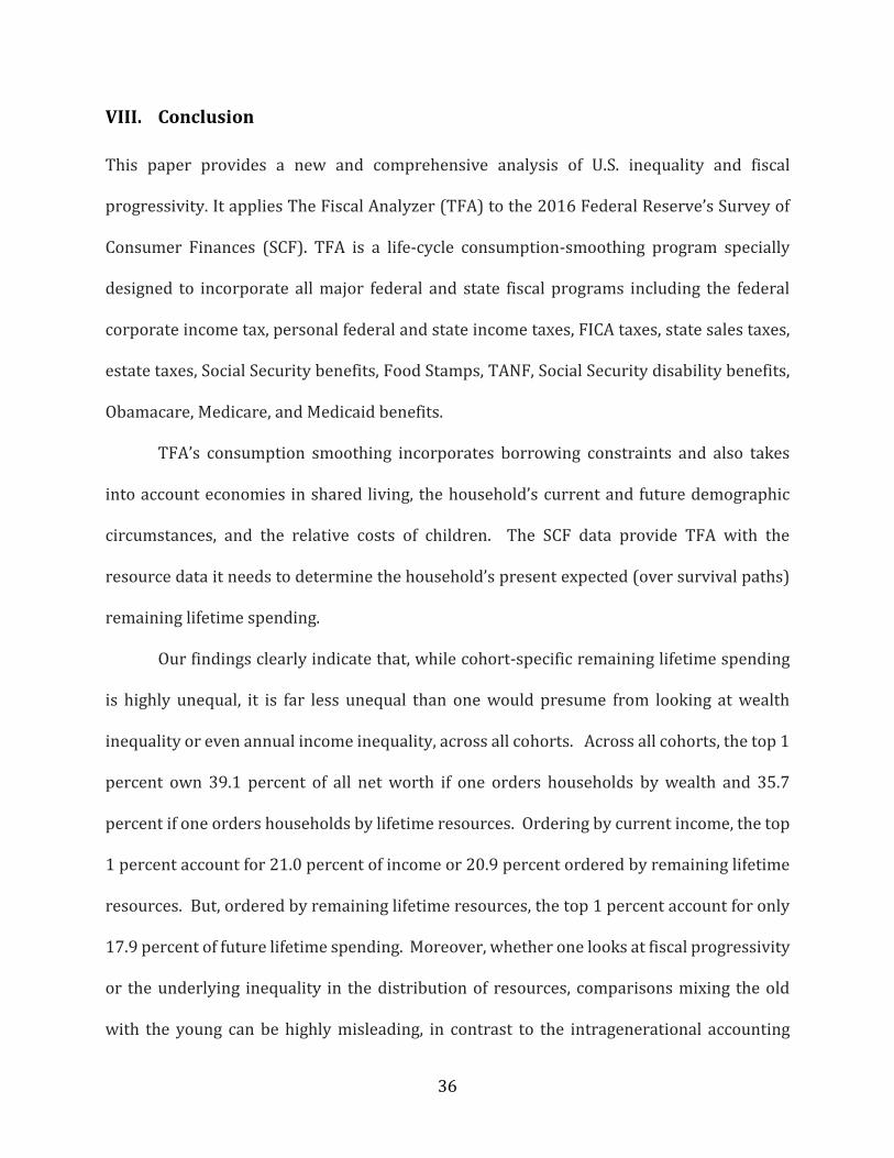
For the cohort age 40 to 49 in 2019, Figure 3 shows that each dollar of pre-tax

remaining lifetime resources of those in the top 1 percent of the resource distribution is

taxed, on average, at a 34.5 percent rate. For those in the top quintile the average net tax

rate is 28.4 percent rate. For those in the bottom quintile, every dollar of pre-tax resources

is matched by a 46.6 percent net subsidy. The figure also shows, as discussed below, the

inability of current-year net tax rates to even roughly capture fiscal progressivity at the

bottom end of the resource distribution.

Figure 4 shows the impact on RLS of this progressive pattern of net tax rates. The

figure compares the average level of spending (the present value of remaining lifetime

spending, both discretionary and non-discretionary) within each quintile with and without

fiscal policy. Although spending remains highly unequal even with the application of fiscal

policy, it’s significantly less unequal as a result of fiscal policy, in accordance with Figure 3’s

findings. For example, RLS among the top 1 percent is reduced by over one third by the U.S.

fiscal system. As the figure shows, this still leaves massive inequality in average remaining

25

lifetime spending among, say, the bottom quintile and the top 1 percent. But this differential

would be far greater absent fiscal policy.

Figure 5 translates the remaining lifetime spending levels in Figure 4 into shares of

overall spending by group, and juxtaposes these shares with the corresponding shares of

wealth for these groups. Spending is much more equally distributed than is wealth. The top

1, 5, and 20 percent of the 40-49 year-old cohort own 34.1 percent, 60.7, and 82.0 percent of

all wealth (financial assets plus housing and other real estate equity less financial liabilities),

respectively. But these three groups account for only 14.5, 28.0, and 50.1 percent of the

cohort’s spending power as measured by remaining lifetime resources net of remaining

lifetime net taxes. Those in the lowest quintile have only 0.6 percent of wealth but 7.3

percent of their cohort’s total spending power. The next three quintiles also each account

for much more of the cohort’s spending power than of its wealth holdings.

Why Is Projected Spending Less Unequal Than Wealth?

Wealth is only one of four determinants of remaining lifetime spending. The others are

remaining lifetime labor earnings, remaining lifetime gross taxes, and remaining lifetime

gross transfer payments. Wealth is certainly very unequally distributed. But, as figure 6

shows, remaining lifetime earnings is less unequally distributed. While those in the top 1

percent hold 34.1 percent of all wealth, they account for just 13.7 percent of remaining

lifetime earnings. Surprisingly, transfer payments are also skewed toward the rich, albeit far

less dramatically: the top 1 percent of 40-49 year olds account for 1.2 percent of future

transfer payments received. The remaining spending component – remaining lifetime tax

payments – is heavily skewed against the rich. The top 1 percent accounts for 20.4 percent

of all tax payments.

26

Taxes remain highly skewed further down the resource distribution. The top 5

percent of 40-49 year olds account for 35.6 percent of all remaining lifetime tax payments,

and the top 20 percent for 60.2 percent. Consistent with this high share of taxes at the top

(and the relative unimportance of transfers in terms of redistribution), each of the bottom

four quintiles has a share of spending that exceeds its share of resources. This can be seen

by comparing findings in Figures 3 and 5. To be precise, the lowest quintile has 4.0 percent

of the resources, but 7.3 percent of the spending. The second quintile has 8.8 percent of the

resources, but 10.4 percent of the spending. The third quintile has 12.7 percent of the

resources, but 13.7 percent of the spending. And the fourth quintile has 18.2 percent of the

resources but 18.5 percent of the spending.

From this perspective, the top quintile is redistributing to all the other quintiles via

the tax and transfer system. The result is a spending share of 50.1 percent among the top

quintile compared to a resource share of 56.3 percent. The absolute gap is nearly as large

for the top 5 percent, who account for 32.8 percent of all resources, but just 28.0 percent of

all spending. The top 1 percent has 17.9 percent of all resources, but accounts for only 14.5

percent of all spending.

Clearly the U.S. fiscal system is highly progressive. Whether it is sufficiently

progressive or overly progressive is a judgment that can be made only by weighing the social

value of such redistribution against its efficiency costs. But whatever one makes of these

findings, on thing is clear -- assessing economically relevant inequality – inequality in

spending power – requires understanding all the elements determining spending. Focusing

exclusively or even primarily on inequality in wealth or current-year income, or, for that

matter, on inequality in some other component of spending power, such as claims to

27

Medicaid, can present a very incomplete and, hence, distorted picture of true overall

inequality.

The Inadequacy of Current-Year Net Tax Rates

Figure 3 shows that current-year net tax rates are an imperfect indicator of the longer-run

fiscal burden represented by average remaining lifetime net tax rates. The figure compares

current-year average tax rates to lifetime net tax rates for 40-49 year-olds.23 The figure

shows that current-year average net tax rates can understate the degree of progressivity in

the U.S. fiscal system (the rate of ascent of the bars in the figure) as well as the average levels

of net taxation of the rich and, especially, net subsidization of the poor. The lowest quintile’s

lifetime resources are subsidized, on average, at a 46.6 percent rate. But its average current-

year net subsidy rate is only 9.8 percent. For all of the remaining quintiles, too, the average

current-year net tax rates are higher than the average lifetime net tax rate, but the difference

declines steadily as one moves up the income distribution.

Components of Taxes and Transfers

The fiscal progressivity of the U.S. federal system reflects a combination of different tax and

transfer components. Figure 7 shows the contribution of each component to the overall net

taxes of the 40-49 year-old cohort. For the top quintile, the federal income tax accounts for

more than half of all tax payments, whereas for all other quintiles, the payroll tax is the

largest tax component. This regressivity of the payroll tax is, of course, balanced by the

progressive pattern of payroll-tax funded Social Security and Medicare benefits. While Social

Security benefits grow in size across income quintiles, they do so at a slower rate than

23 Current-year net tax rates equal current-year taxes net of transfers divided by current-year income, measured as current-year labor income plus the imputed rate of return on assets multiplied by assets.

28

lifetime resources. This is even truer of Medicare, which increases across lifetime resources

groups at a slower rate (the increase due in part to the greater longevity of higher-income

individuals). However, substantial progressivity is provided by the other transfers

associated with health care, namely Medicaid and the subsidies under the Affordable Care

Act (Obamacare), which are large in size and highly concentrated in the bottom quintile of

the lifetime resource distribution.

2. Findings for Other Cohorts

Figures 8 and 9 show current-year and lifetime tax rates for those in other cohorts, aged 20-

29 and 60-69. For the younger cohort, in Figure 8, lifetime net tax rates are higher, primarily

because of the longer lag until the receipt of large transfer payments in old age. Also, the

progressivity of lifetime net tax rates and current-year net tax rates have a less clear ranking,

the latter being less progressive at the top, but more progressive at the bottom. This is likely

due to the fact that there is a much lower rank correlation in this cohort between lifetime

resources and current income – many of those at the top of the current income distribution

will not be near the top of the lifetime resource distribution and, therefore, are less subject

to higher taxes. This lower rank correlation relates to the longer remaining horizon for labor

earnings as well as the relatively greater importance of wealth in determining inequality

among the young.

This ambiguity disappears when one looks at the same tax-rate comparison for 60-

69 year-olds, in Figure 9. Here, current-year net tax rates are low because of lower labor

force participation, and remaining lifetime net tax rates are lower still because of the

impending receipt of substantial old-age transfer payments. These payments, taking all

programs together, are substantially progressive, making the decline in net tax rates as one

29

moves from right to left in the figure far greater for the lifetime net tax rate series than for

the current-year net tax rate.

VI. Evaluating the Impact of the Tax Cuts and Jobs Act (TCJA)

The TCJA, enacted in late 2017, was the most significant change in the federal income tax

since the Tax Reform Act of 1986. Among its key provisions were a reduction in the

corporate tax rate from 35 percent to 21 percent, a reduction in individual tax rates,

increasing the standard deduction, capping of the itemized deduction for state and local

taxes, eliminating the corporate Alternative Minimum Tax (AMT), scaling back the individual

AMT, and a new reduced tax rate on qualifying non-corporate businesses.

Many of TCJA’s tax provisions become less favorable to taxpayers over the course of

the 10-year budget period. In addition, many of its individual tax cut provisions are set to

expire by the end of the decade. These features appear to have been included simply to meet

arbitrary budget targets within the budget period and to limit the growth in projected

deficits beyond the budget period. Meeting the budget targets and limiting future projected

deficits were needed to permit passage of the bill with a simple majority in the Senate.

However, there was no coherent policy reason offered for such temporary provisions, nor

are we aware of any. Consequently, in this analysis, we assume TCJA’s provisions are

permanent. This assumption is important to keep in mind when interpreting our results and

comparing them with those of other studies that adhere strictly to the letter of TCJA’s law.

In modeling the TCJA, we reduced our corporate tax rate, by 12.4 percent. This is the

average, over the next five years, due to TCJA, in the Joint Committee on Taxation’s projected

30

corporate tax revenue loss divided by the 2017 NIPA estimate of corporate tax revenue.24

One useful check of our benchmarking procedure is to compare our results with those of the

Joint Committee on Taxation, which are based on tax return data, albeit for 2013. Table 2

shows average current-year gross tax rates under old law, under the TCJA, and the change

between the two, from JCT (2017) and according to our calculations, where we adhere as

closely as possible to JCT’s income classification and income and tax definitions. 25 As the

table shows, our gross tax rate measures are relatively close to JCT’s. Indeed, the correlation

coefficient between our TCJA average rates and the JCT’s across the income categories in the

table is 96.0 percent. Moreover, like JCT, we find an increase in percentage tax cuts as income

increases, with the exception of the highest income group, although the upward trend is less

pronounced in our analysis. The fact that we are able to come reasonably close to the JCT’s

analysis of progressivity with the SCF data suggests that it is not differences in data, but

differences in methodology that underlie our different findings about fiscal progressivity and

inequality.

Figure 10 shows average and current year remaining lifetime net tax rates for the age

40-49 cohort under old law, which can be compared to figure 3 to see the distributional

impact of the TCJA based on these two measures. The lifetime net tax rate reductions by

quintile, in percentage points, are 1.1, 1.5, 1.7, 1.6, and 1.3, with reductions for the top 5 and

24 https://www.jct.gov/publications.html?func=startdown&id=5053 25 https://www.jct.gov/publications.html?func=startdown&id=5054. We are unable to include certain components of JCT’s expanded income measure, including worker’s compensation, alternate minimum tax preference items, individual share of business taxes, and excluded income of U.S. citizens living abroad. The JCT is also using 2013 IRS data, which is the latest such data available, whereas our SCF data reference either 2015 or 2016. Our approach and the JCT’s both assume that the incidence of the corporate income tax falls 100 percent on owners of capital. The JCT also assumes that nearly 10 percent of corporate income accrues to foreign owners, whose burden is excluded from their calculation (JCT, 2013). We make no adjustment in our analysis for foreign ownership.

31

top 1 percent of 1.2 and 0.8 percentage points, respectively. The current-year net tax rate

reductions for the same groups are 1.6, 1.4, 1.4, 1.4, 1.3, 1.2, and 0.6.26 Hence, the patterns

are generally similar, although the net tax cut in the lowest income quintile is lower on a

remaining lifetime basis than for the current year, and the progressivity of the TCJA is

somewhat lower as well.

Note that focusing on net rather than gross tax rates, holding age fixed within a range,

and partitioning by resource-percentile group produces, in this case, a different assessment

of TCJA’s progressivity than that suggested by the JCT’s analysis or our version of the JCT’s

analysis. On a current-year net tax rate basis, the reform, for forty year olds, is progressive.

On a remaining lifetime net tax rate basis, it favors the middle class over the poor and the

rich. Precisely how much of the difference in these and our version of JCT’s results arise from

these other factors is another subject for future research.

A similar relative pattern is present for other cohorts. For 20-29 year olds, for

example, the lifetime net tax rate reductions, from the lowest quintile to the highest

percentile, are 1.7, 1.7, 2.0, 1.9, 1.0, 0.7, and 0.1 percentage points, whereas the reductions in

current net tax rates for the same respective groups are 2.2, 1.8, 2.1, 2.0, 1.3, 0.5, and -0.3

percentage points. Again, the net tax rate reduction is higher at the bottom and lower at the

top (in this case, a small increase) for current tax rates. One factor likely underlying this

greater similarity across resource groups for the remaining lifetime net tax rates is that

current-income differences overstate differences in lifetime resources, even when one is

segregating by age group, because of the assumed process for labor earnings. One difference

26 Note that the decline in net tax rate reductions beginning in the top quintile is not inconsistent with the results in Table 2, given that the top quintile includes those in the highest income group, who experience a lower tax rate reduction.

32

among 20-29 year olds is that that both sets of net tax rate reductions appear more

progressive across income groups in terms of the relative net tax rate reductions for low-

and high-resource individuals. We conjecture that this difference may relate to the

difference in dispersion of all lifetime resources across groups in the two cohorts; 20-29 year

olds have a lower concentration of lifetime resources at the top but a stronger concentration

of wealth. We will explore the reasons for this difference in subsequent drafts.

VII. Sensitivity Analysis

Our results rely on many assumptions, and it is useful to consider the influence of particular

assumptions on our findings.

A. Differential Mortality

Auerbach et al. (2017), on which our mortality assumptions are based, focuses on the decline

in progressivity of old-age transfer payments with the increasing income-longevity link. As

old-age transfer payments are survival-based, higher mortality translates into lower

benefits, in present value, even in cases, such as Social Security, where the underlying annual

payments are progressive, delivering a higher replacement rate for retirees with lower

lifetime incomes. However, mortality affects not only the receipt of transfer payments, but

also the payment of taxes.

To gauge the impact of these effects, we simulate outcomes under the assumption that

all individuals of each age, gender and cohort have the same life expectancy as those in the

top resource quintile (where, as discussed above, resources are based on an AIME

calculation, in line with the groupings used in deriving the mortality estimates). Figure 11

displays the results of this simulation for the 40-49 year old cohort, which may be compared

33

to the results in Figure 3, which differ only with respect to the mortality assumption. For

this cohort, the lifetime net tax rate falls for those in two lowest resource quintiles, but

generally rises in the other resource groups, suggesting that the relative importance of

higher future net taxes is larger as income rises, consistent with the redistributive nature of

old-age transfer programs.27

For 60-69 year olds, depicted in Figure 12 (which can be compared to Figure 9)

lifetime net tax rates are lower for all resource groups except the top 5 and 1 percent, for

whom there is no change. For this cohort, the longer period of transfer-payment receipt

dominates, except at the top, where most individuals have the same mortality assumptions

in the two cases.28

We conclude that ignoring differential mortality, though not having a large

quantitative impact on our estimates of progressivity, would make the system look more

progressive than it is by making the old-age transfer system appear more generous to those

in lower resource groups.

B. A Lower Rate of Return on Saving

The rate of return before all taxes (including corporate taxes) used in our results is based on

the historical return to capital, as discussed above. However, many have suggested that

future rates of return may be lower, for example because of the demographic transition

27 Note that these tables compare groups based on the ranking of lifetime resources under the respective scenarios, which will differ somewhat across the two cases. This explains why current-year tax rates differ across the scenarios, because current income and current taxes are the same for each individual in the two cases. 28 Note that these results for 60-69 year olds must be interpreted with some care, as the changes in mortality affect the composition of the population. This is not the case for 40-49 year olds, as all changes in mortality are assumed to begin at age 50.

34

leading, at least in the developed world, to increases in capital labor ratios. To consider the

potential impact on our findings, we repeat our analysis under the assumption that the real,

before-tax return to capital is 4 percent, rather than 6.371 percent.

Figure 13 presents the results of this simulation for the net tax rates faced by 40-49

year-olds, which can be compared to the base case simulations in Figure 3. Current-year tax

rates are higher for those in the top resource groups, because a smaller share of these groups’

current income is accounted for by capital income, which faces a lower average current-year

tax rate than does labor income. On a lifetime basis, however, the pattern is less clear. While

the top 1 percent still face a higher average tax rate, there is little net impact for the top 5

percent, and lower average net tax rates for the other groups. This is due to the fact that the

lower discount rate associated with a lower rate of return increases the present value of

future old-age transfer payments, thereby reducing the present value of lifetime net taxes.

Thus, from the remaining lifetime perspective, assuming a lower rate of return increases the

progressivity of the fiscal system. These effects on lifetime net tax rates are even more

pronounced for 60-69 year olds (see Figure 14, which may be compared to Figure 9), where

even the top 5 percent of the resource distribution experience a drop in remaining lifetime

net tax rates. For this cohort, the value of transfer payments looms larger as a component of

net tax rates.

C. A Voluntary Bequest Motive

Our consumption smoothing algorithm assumes that households seek the highest, level of

consumption possible, given resources and borrowing constraints. This means that

bequests occur as a consequence of dying before the maximum age, to the extent that assets

are not annuitized. But the algorithm does not provide for intentional bequests. While there

35

is considerable uncertainty about the motivations for observed bequests, we consider the

impact of introducing a voluntary bequest motive. In our model, a simple way of introducing

this motive is to assume that there is a ceiling on the annual amount of spending that a

household will undertake, so that wealthy households, who under the consumption-

smoothing algorithm would exceed the ceiling, simply roll assets forward. This results in

intentional bequests among those wealthy enough to hit the ceiling.

Simulations under this alternative assumption, for the case of an annual ceiling on the

standard of living of $5 million, has a minor impact on estimated lifetime average net tax

rates, although the changes are consistent with what one would expect. Among 40-49 year-

olds, those in the top 1 percent of resources experience a small increase (about one half of a

percent) in their lifetime net tax rates. This results from the fact that, with more future asset

accumulation, there will be more capital income taxes and estate taxes to pay. The result is

more pronounced for 60-69 year-olds (an increase of about 2 percent in the remaining

lifetime tax rate), as the higher estate tax payments loom closer in the future. Again, this

modification of our assumptions results in greater progressivity in the fiscal system, from a

remaining-lifetime perspective.

D. Cheaper Consumption in Retirement and Different Time Preference Rates

We also consider and found no material difference in our findings from the assumptions that

households wish to have their living standards per effective adult rise or fall annually by 2

percent or that households plan for their consumption outlays to drop, other things equal,

by 20 percent once they reach retirement, reflecting the potential of lower consumption cost

in retirement raised by Aguiar and Hurst (2005).

36

VIII. Conclusion

This paper provides a new and comprehensive analysis of U.S. inequality and fiscal

progressivity. It applies The Fiscal Analyzer (TFA) to the 2016 Federal Reserve’s Survey of

Consumer Finances (SCF). TFA is a life-cycle consumption-smoothing program specially

designed to incorporate all major federal and state fiscal programs including the federal

corporate income tax, personal federal and state income taxes, FICA taxes, state sales taxes,

estate taxes, Social Security benefits, Food Stamps, TANF, Social Security disability benefits,

Obamacare, Medicare, and Medicaid benefits.

TFA’s consumption smoothing incorporates borrowing constraints and also takes

into account economies in shared living, the household’s current and future demographic

circumstances, and the relative costs of children. The SCF data provide TFA with the

resource data it needs to determine the household’s present expected (over survival paths)

remaining lifetime spending.

Our findings clearly indicate that, while cohort-specific remaining lifetime spending

is highly unequal, it is far less unequal than one would presume from looking at wealth

inequality or even annual income inequality, across all cohorts. Across all cohorts, the top 1

percent own 39.1 percent of all net worth if one orders households by wealth and 35.7

percent if one orders households by lifetime resources. Ordering by current income, the top

1 percent account for 21.0 percent of income or 20.9 percent ordered by remaining lifetime

resources. But, ordered by remaining lifetime resources, the top 1 percent account for only

17.9 percent of future lifetime spending. Moreover, whether one looks at fiscal progressivity

or the underlying inequality in the distribution of resources, comparisons mixing the old

with the young can be highly misleading, in contrast to the intragenerational accounting

37

done here, which compares remaining lifetime spending and fiscal redistribution within

cohorts.

Assessing inequality and fiscal progressivity based on current income and gross, let

alone net tax rates is likely to misstate both and very significantly. The distribution of

current income differs from that of remaining lifetime spending and current-year net tax

rates generally understate the degree of progressivity of the tax and transfer system. This is

true even if one considers net tax rates within generations. One can also reach different

conclusions about the progressivity of tax reforms, as our analysis of the Tax Cuts and Jobs

Act shows.

There are many directions for future research, including understanding changes over

time in spending inequality and fiscal progressivity and comparing spending inequality and

fiscal progressivity across countries. Also, our analysis applies to the current fiscal system,

projected forward, even though there is a general consensus that major changes will be

needed to sustain fiscal balance. How fiscal balance is restored will have an impact on our

measures, depending on the distribution of fiscal adjustments within and across generations.

This study’s bottom line, however, will remain. Inequality and fiscal progressivity

shouldn’t be studied in isolation or in a piecemeal fashion, nor can they be accurately

assessed by combining very different age cohorts in the analysis.

References

Acemoglu, Daron and David Autor. 2011. “Skills, Tasks and Technologies: Implications for Employment and Earnings.” Handbook of Labor Economics. 4(B), 1043-1171. Aguiar, Mark and Eric Hurst. 2005. “Consumption vs Expenditure.” Journal of Political Economy, October 2005, 113(5), 919-948.

38

Altig, David, Alan J. Auerbach, Laurence J. Kotlikoff, Kent A. Smetters and Jan Walliser. 2001. “Simulating Fundamental Tax Reform in the United States.” American Economic Review 91(3), 574-595. Auerbach, Alan J., Kerwin K. Charles, Courtney C. Coile, William Gale, Dana Goldman, Ronald Lee, Charles M. Lucas, Peter R. Orszag, Louise M. Sheiner, Bryan Tysinger, David N. Weil, Justin Wolfers, and Rebecca Wong. 2017. "How the Growing Gap in Life Expectancy May Affect Retirement Benefits and Reforms," The Geneva Papers on Risk and Insurance 42(3), 475-499, July. Auerbach, Alan J. and Laurence J. Kotlikoff. 1987. Dynamic Fiscal Policy. Cambridge, England: Cambridge University Press. Auerbach, Alan J., Jagadeesh Gokhale, and Laurence J. Kotlikoff. 1991. “Generational Accounts: A Meaningful Alternative to Deficit Accounting.” Tax Policy and the Economy. NBER Volume 5. January. 55-106. Bengtsson, Niklas, Bertil Holmlund, and Daniel Waldenstrom. 2016. “Lifetime versus Annual Tax and Transfer Progressivity: Sweden, 1968-2009. The Scandinavian Journal of Economics 118(4), 619-645. Congressional Budget Office. 2014. The Distribution of Household Income and Federal Taxes, 2011, November 12. Congressional Budget Office. 2016. Trends in Family Wealth, 1989-2013. August. Favreault, Melissa M., Karen E. Smith, and Richard W. Johnson. "The Dynamic Simulation of Income Model (DYNASIM)." Urban Institute Program on Retirement Policy Research Report (2015). Fullerton, Don and Diane Lim Rogers. 1993. Who Bears the Lifetime Tax Burden? Washington: The Brookings Institution. Goda, Gopi Shah, John B. Shoven, and Sita Nataraj Slavov. 2011. “Differential Mortality by Income and Social Security Progressivity.” Explorations in the Economics of Aging (D. Wise, ed.). Chicago: University of Chicago Press. 189-204. Goldin, Claudia and Lawrence Katz. 2008. The Race Between Education and Technology. Cambridge: Harvard University Press. Gottschalk, Peter, and Robert Moffitt. 1995. “Trends in the Covariance Structure of Earnings in the US: 1969-1987.” Working Paper, Boston College Department of Economics. Green, Jerry and Laurence J. Kotlikoff. 2008. “The General Relativity of Fiscal Language,” in Institutional Foundations of Public Finance. Alan J. Auerbach and Daniel Shaviro, eds. 241-56.

39

Harberger, Arnold C. 1962. “The Incidence of the Corporation Income Tax, Journal of Political Economy 70 (3), June, 215-240. Joint Committee on Taxation. 2013. Modeling the Distribution of Business Income. JCX-14-13. October 13. https://www.jct.gov/publications.html?func=startdown&id=4528 Joint Committee on Taxation. 2017. Distributional Effects of the Conference Agreement for H.R.1 “The Tax Cuts and Jobs Act.” JCX-68-17. December 18. https://www.jct.gov/publications.html?func=startdown&id=5054 Kopczuk, Wojciech, Emmanuel Saez, and Jae Song. 2010. “Earnings Inequality and Mobility in the United States: Evidence from Social Security Data Since 1937. The Quarterly Journal of Economics. February. 91-128. Kotlikoff, Laurence J. 1984. “Deficit Delusion.” The Public Interest, 84, Summer. 53-65. http://www.kotlikoff.net/sites/default/files/deficit_delusion_0.pdf Kotlikoff, Laurence J. 1988. “The Deficit Is Not a Well Defined Measure of Fiscal Policy.” Science. August 12. 241. 791-95. Kotlikoff, Laurence J. 2002. “Generational Policy.” Handbook of Public Economics. Alan J. Auerbach and Martin Feldstein, eds. 4, 1873-1932. Laibson, David. 1997. “Golden Eggs and Hyperbolic Discounting,” The Quarterly Journal of Economics 112(2), 443-477. Meghir, Costas and Luigi Pistaferri. 2011. “Earnings, Consumption and Life Cycle Choices,” in D. Card and O. Ashenfelter, eds., Handbook of Labor Economics, vol. 4b, 773-854. Meyer, Bruce D., and James X. Sullivan. 2017. “Consumption and Income Inequality in the US Since the 1960s.” No. w23655. National Bureau of Economic Research. Pechman, Joseph A. and Benjamin A. Okner. 1974. Who Bears the Tax Burden. Washington: The Brookings Institution. Piketty, Thomas, Emmanuel Saez, and Gabriel Zucman. 2018. “Distributional National Accounts: Methods and Estimates for the United States,” Quarterly Journal of Economics 133(2), 553-609. Poterba, James M. 1989. “Lifetime Incidence and the Distributional Burden of Excise Taxes.” American Economic Review. 79(2), 325-330.

Table 1 Comparing Lifetime-Resource and Current-Income Distributions, Ages 40 – 49

Share In Each Current Income Percentile

Lifetime Resource Percentile Lowest Second Third Fourth Highest

Top 5%

Top 1%

Lowest 85.2% 8.6% 2.0% 3.7% 0.5% 0.0% 0.0% Second 16.8% 67.2% 11.4% 1.4% 3.2% 0.0% 0.0% Third 0.3% 25.1% 55.9% 17.3% 1.4% 0.0% 0.0%

Fourth 0.0% 0.8% 32.4% 56.4% 10.4% 0.0% 0.0% Highest 0.0% 0.0% 0.5% 9.9% 89.6% 50.8% 23.3% Top 5% 0.0% 0.0% 0.0% 0.0% 100.0% 93.7% 46.3% Top 1% 0.0% 0.0% 0.0% 0.0% 100.0% 100.0% 97.6%

* Highest percentage in each row is green.

Table 2

Distributional Effects of the Tax Cuts and Jobs Act

TFA Estimates JCT (2017a) Estimates

Income Category

Avg. Tax Rate

Under Present

Law

Avg. Tax Rate

Under TJCA Change

Avg. Tax Rate Under

Present Law

Avg. Tax Rate

Under TJCA Change

Less than 10,000 14.04% 12.62% -1.42% 9.10% 8.60% -0.50% 10,000 to 20,000 3.33% 2.56% -0.77% -0.70% -1.20% -0.50% 20,000 to 30,000 1.64% 0.56% -1.09% 3.90% 3.40% -0.50% 30,000 to 40,000 6.45% 5.18% -1.27% 7.90% 7.00% -0.90% 40,000 to 50,000 10.69% 9.40% -1.29% 10.90% 9.90% -1.00% 50,000 to 75,000 11.79% 10.44% -1.35% 14.80% 13.50% -1.30%

75,000 to 100,000 14.57% 13.02% -1.55% 17.00% 15.60% -1.40% 100,000 to 200,000 18.92% 17.17% -1.76% 20.90% 19.40% -1.50% 200,000 to 500,000 26.00% 23.83% -2.17% 26.40% 23.90% -2.50%

500,000 to 1,000,000

34.35% 32.17% -2.19% 30.90% 27.80% -3.10% 1,000,000 and over 38.40% 37.42% -0.98% 32.50% 30.20% -2.30%

Figure 1

Figure 2

-0.8%

0.4% 2.4%7.7%

90.3%

67.8%

39.1%

Lowest Second Third Fourth Highest Top 5% Top 1%

Share of Net Wealth by Net Wealth Percentile, Ages 20 - 79

2.0%5.9%

10.2%17.0%

64.8%

40.2%

22.1%

3.1%7.5%

11.7%17.3%

60.4%

37.7%

20.9%

Lowest Second Third Fourth Highest Top 5% Top 1%

Lifetime Resources and Current Income by Resource Percentile, Ages 20 - 79

Share of Lifetime Resources Share of Current Income

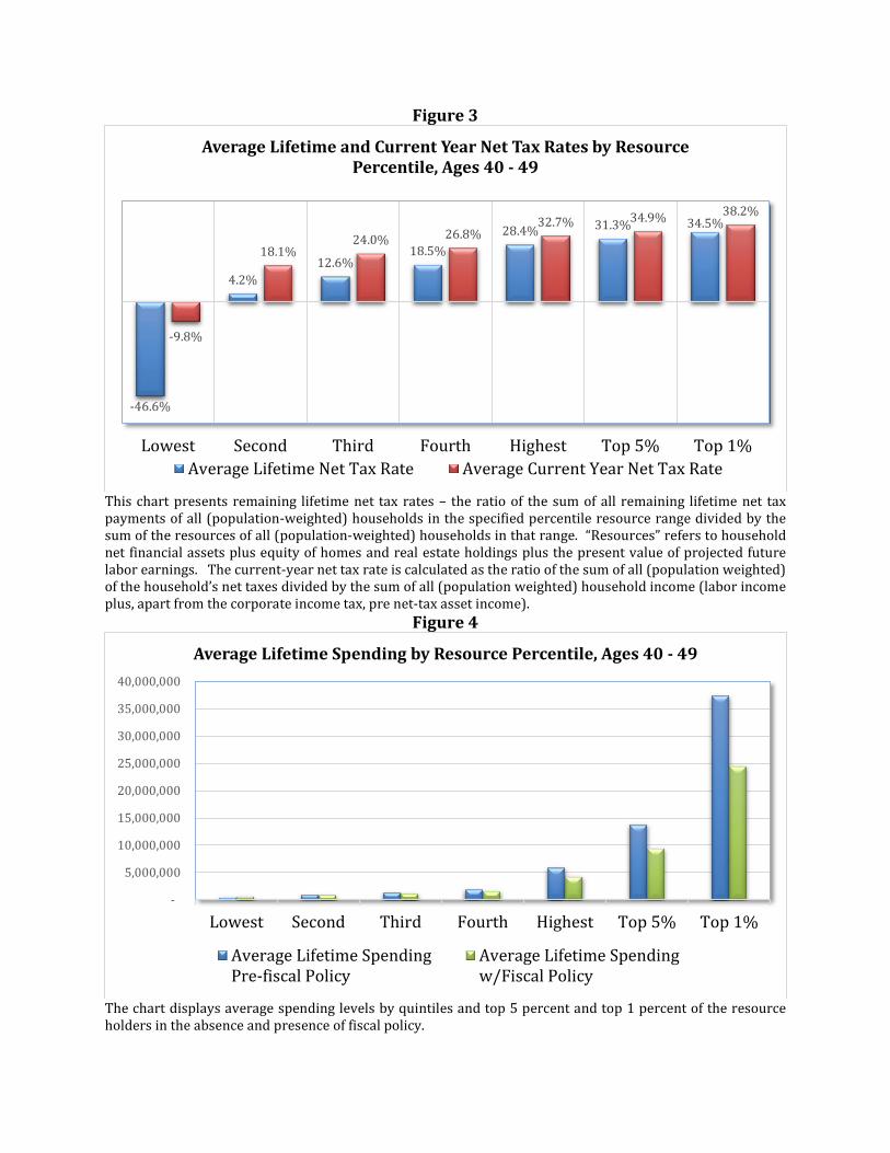
Figure 3

This chart presents remaining lifetime net tax rates – the ratio of the sum of all remaining lifetime net tax payments of all (population-weighted) households in the specified percentile resource range divided by the sum of the resources of all (population-weighted) households in that range. “Resources” refers to household net financial assets plus equity of homes and real estate holdings plus the present value of projected future labor earnings. The current-year net tax rate is calculated as the ratio of the sum of all (population weighted) of the household’s net taxes divided by the sum of all (population weighted) household income (labor income plus, apart from the corporate income tax, pre net-tax asset income).

Figure 4

The chart displays average spending levels by quintiles and top 5 percent and top 1 percent of the resource holders in the absence and presence of fiscal policy.

-46.6%

4.2%12.6%

18.5%28.4% 31.3% 34.5%

-9.8%

18.1%24.0% 26.8%

32.7% 34.9% 38.2%

Lowest Second Third Fourth Highest Top 5% Top 1%

Average Lifetime and Current Year Net Tax Rates by Resource Percentile, Ages 40 - 49

Average Lifetime Net Tax Rate Average Current Year Net Tax Rate

Lowest Second Third Fourth Highest Top 5% Top 1% -

5,000,000

10,000,000

15,000,000

20,000,000

25,000,000

30,000,000

35,000,000

40,000,000

Average Lifetime Spending by Resource Percentile, Ages 40 - 49

Average Lifetime SpendingPre-fiscal Policy

Average Lifetime Spendingw/Fiscal Policy

Figure 5

The chart displays asset and spending shares of those in the five quintiles of the distribution of resources as well as those in the top 5 percent and top 1 percent.

Figure 6

0.6% 3.0% 5.3%9.2%

82.0%

60.7%

34.1%

7.3% 10.4% 13.7%18.5%

50.1%

28.0%

14.5%

Lowest Second Third Fourth Highest Top 5% Top 1%

Share of Net Wealth and Lifetime Spending by Resource Percentile, Ages 40 - 49

Share of Net Wealth Share of Lifetime Spending

0.0%

10.0%

20.0%

30.0%

40.0%

50.0%

60.0%

70.0%

80.0%

90.0%

Lowest Second Third Fourth Highest Top 5% Top 1%

Share of Net Wealth Share of Lifetime IncomeShare of Lifetime Transfer Payments Share of Lifetime Taxes

Figure 7

0 500,000 1,000,000 1,500,000 2,000,000 2,500,000

Lowest

Second

Third

Fourth

Highest

Average Remaining Lifetime Taxesby Resource Percentile, Ages 40 - 49

Federal Tax State Tax FICA Tax

Sales Tax Corporate Tax Medicare B Premiums

0 50,000 100,000 150,000 200,000 250,000 300,000 350,000

Lowest

Second

Third

Fourth

Highest

Average Remaining Lifetime Transfer Paymentsby Resource Percentile, Ages 40 - 49

Social Security Benefits Medicare Medicaid

SSDI SSI TANF

Food Stamps ACA

Figure 8

Figure 9

-10.5%

16.3%

24.4%28.4%

35.3% 36.3% 35.9%

-6.1%

13.3%

20.0%25.0%

33.1% 35.3% 37.0%

Lowest Second Third Fourth Highest Top 5% Top 1%

Average Lifetime and Current Year Net Tax Rates by Resource Percentile, Ages 20 - 29

Average Lifetime Net Tax Rate Average Current Year Net Tax Rate

-438.7%

-126.2%-59.5%

-22.5%

12.1% 17.4% 20.6%

-247.3%

-51.3%-7.7%

13.8% 26.2% 29.1% 30.6%

Lowest Second Third Fourth Highest Top 5% Top 1%

Average Lifetime and Current Year Net Tax Rates by Resource Percentile, Ages 60 - 69

Average Lifetime Net Tax Rate Average Current Year Net Tax Rate

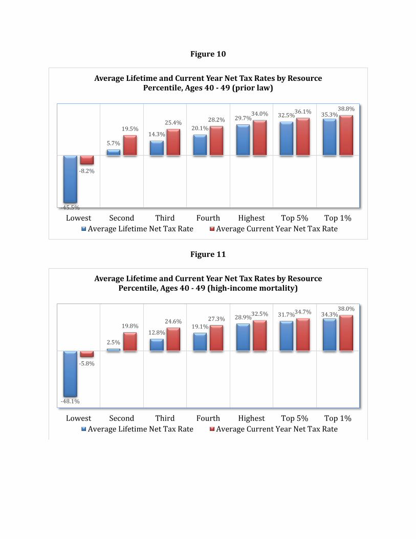
Figure 10

Figure 11

-45.5%

5.7%14.3%

20.1%29.7% 32.5% 35.3%

-8.2%

19.5%25.4% 28.2%

34.0% 36.1% 38.8%

Lowest Second Third Fourth Highest Top 5% Top 1%

Average Lifetime and Current Year Net Tax Rates by Resource Percentile, Ages 40 - 49 (prior law)

Average Lifetime Net Tax Rate Average Current Year Net Tax Rate

-48.1%

2.5%12.8%

19.1%28.9% 31.7% 34.3%

-5.8%

19.8%24.6% 27.3%

32.5% 34.7% 38.0%

Lowest Second Third Fourth Highest Top 5% Top 1%

Average Lifetime and Current Year Net Tax Rates by Resource Percentile, Ages 40 - 49 (high-income mortality)

Average Lifetime Net Tax Rate Average Current Year Net Tax Rate

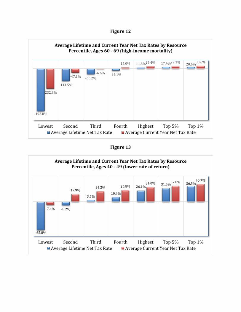
Figure 12

Figure 13

-495.0%

-144.5%

-66.2%-24.1%

11.8% 17.4% 20.6%

-232.3%

-47.1%-6.6%

15.0% 26.4% 29.1% 30.6%

Lowest Second Third Fourth Highest Top 5% Top 1%

Average Lifetime and Current Year Net Tax Rates by Resource Percentile, Ages 60 - 69 (high-income mortality)

Average Lifetime Net Tax Rate Average Current Year Net Tax Rate

-65.8%

-8.2%

3.5%10.4%

26.1% 31.5% 36.5%

-7.4%

17.9%24.2% 26.8%

34.0% 37.0% 40.7%

Lowest Second Third Fourth Highest Top 5% Top 1%

Average Lifetime and Current Year Net Tax Rates by Resource Percentile, Ages 40 - 49 (lower rate of return)

Average Lifetime Net Tax Rate Average Current Year Net Tax Rate

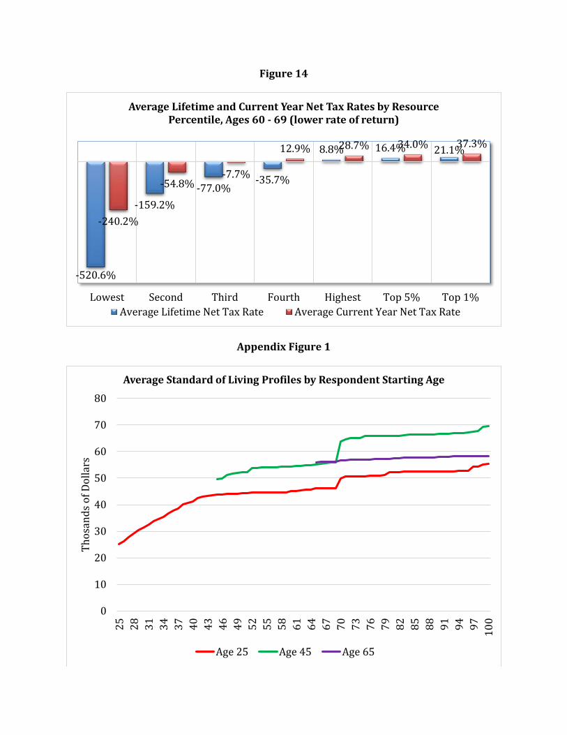
Figure 14

Appendix Figure 1

-520.6%

-159.2%-77.0%

-35.7%

8.8% 16.4% 21.1%

-240.2%

-54.8%-7.7%

12.9% 28.7% 34.0% 37.3%

Lowest Second Third Fourth Highest Top 5% Top 1%

Average Lifetime and Current Year Net Tax Rates by Resource Percentile, Ages 60 - 69 (lower rate of return)

Average Lifetime Net Tax Rate Average Current Year Net Tax Rate

0

10

20

30

40

50

60

70

80

25 28 31 34 37 40 43 46 49 52 55 58 61 64 67 70 73 76 79 82 85 88 91 94 97 100

Thos

ands

of D

olla

rs

Average Standard of Living Profiles by Respondent Starting Age

Age 25 Age 45 Age 65