U.S. DEPARTMENT OF THE INTERIOR U.S. GEOLOGICAL SURVEY

Theoretical Models of Heterogeneous Media for Electrical Prospecting Methods with Direct Currents

(Model theorique des milieux heterogenes pour les methodes

de projection electrique a courant stationair)

Published in French in:

Comitetul Geologic, Studii Technice si Economice, Seria D, Nr 2, Imprimeria National, Bucuresti, p 51-71.

By Sabba S. Stefanescu

Translated, edited, and annotated by Adel A.R. Zohdy 1

Introduction by Adel AR. Zohdy1

Open-File Report 95-544

1995

This report has not been reviewed for conformity with the U.S. Geological Survey standards. Opinions

and conclusions expressed herein do not necessarily represent those of the USGS.

1. Box 25046, MS 964, Denver Federal Center, Denver Colorado 80225

INTRODUCTIONBy

Adel A.R. Zohdy

Sabba S. Stefanescu was one of the primary contributors to the study of theoretical electrical methods in geophysical exploration. He published the present paper in 1950 on what is now known as the "a-center" model (Stefanescu, 1950). The paper became a classic as it formed the foundation for many subsequent studies on the same subject. However, one cannot mention Stefanescu's contributions to electrical prospecting without first referring to his 1930 classical contribution where he derived an elegant-integral equation for the electrical potential at a point on the surface of a horizontally stratified ground caused by a point-current electrode placed at the surface of the ground (Stefanescu, in collaboration with Conrad and Marcel Schlumberger, 1930). In the following paragraphs, I will discuss the history and the impact of Stefanescu's 1930 integral equation for horizontal layers and then I will provide a summary of the work that followed the present paper on the a center, from 1950 to 1992.

One year prior to Stefanescu's 1930 publication, Hummel1 (1929 a and b) published two papers on the subject of the electrical-potential distribution in a horizontally-stratified earth model using the method of images. Stefanescu referred to Hummel's work and he also referred to work by Ollendorf (1928) which was published in Die Erdstrome [Earth currents] and he stated that his work follows that of Ollendorf 2 . The kernel function in the integral equation that Stefanescu derived became known as the Stefanescu-kernel function (Kunetz, 1966), and also the integral itself became known as Stefanescu's integral. Kunetz (1966) was the first to show, but without being explicit, that via the redefinition of the integration variable (A,), Stefanescu's integral took the form of a convolution integral. Kunetz may have been the first to derive a convolution filter for the calculation of direct-current electrical soundings, because he was the first to allude to the method of convolution in the very last sentence of his 1966 book, but unfortunately he did not publish his filter coefficients. A few years later, at a meeting of the Society of Exploration Geophysicists, which was held in the late 60's or early 70's, Geza Kunetz told me that he had developed a filter several years earlier and that his filter was composed of three- to four-hundred coefficients with the number of coefficients depending on the accuracy with which one wished to compute a sounding curve. In the 1970's, digital filters with fewer coefficients were designed and published by Ghosh (1971), Anderson (1975), O*Neill (1975), and by many others. These digital filters made it possible to compute direct-current resistivity sounding curves at exceptional speeds on personal computers.

The present paper by Sabba S. Stefanescu was published in 1950 in the Romanian journal "Comitetul Geologic, Studii Technice si Economice, Seria D, Nr. 2, Imprimeria Nationala, Bucuresti, p 57-77." It is the first paper in which Stefanescu stated and defined his ideas about an a-center model, which is an inhomogeneous-isotropic earth

1 Also see Hummel (1932) in the list of references for an English version of the 1929 papers.2 Stefanescu did not provide the first initial of Ollendorf s name nor did he give the year of Ollendorf s publication, but this information is given in the list of references following this introduction.

model that contains a point, a, where the resistivity is zero (infinite conductivity) and from which the resistivity increases radially according to certain rules. The a-center concept made the calculation of apparent resistivities, for electrical soundings and for horizontal profiling, much simpler than for other heterogeneous media. In the following years, several papers were published extending the knowledge about the possible applications of an a-center model. Similar to the present article, almost all the early European literature on the a-center model was written in French, and mostly was published in the "Revue Roumaine de Geologic, Geophysique et Geographic, Serie de Geophysique."

The studies and extensions to the application of the a-center method were made in:

(a) The direct current method, including two- and three-dimensional inversion methods, and two- and three-dimensional resistivity tomography studies using cross-hole data (Petrick and others, 1981; Radulescu, 1967; Sakayama and Shima, 1986; Shima, 1990 a and b; Shima, 1992; Stefanescu D., 1972b; Stefanescu, 1970; Stefanescu, 1987; Stefanescu and others, 1964; Stefanescu and Radulescu, 1965 and 1966; Stefanescu and Stefanescu, 1974; Stefanescu and Tanasescu, 1965; Tran-Ngoc-Toan, 1971).

(b) The magnetic field of a direct current, or the magnetometric resistivity method (Edwards and others, 1978; Stefanescu, 1953; Stefanescu and Tang-Muoi, 1971; Tang- Muoi, 1972).

(c) The induced polarization method (Stefanescu D., 1972a).

In 1990, Sabba S. Stefanescu was awarded Honorary Membership in the Society of Exploration Geophysicists in recognition of his life-long contributions to electrical- geophysical methods.

In this translation, editorial insertions have been added to help the flow of the sentences in English and are placed in brackets. Editorial annotations are indicated as Editor's notes, are written in italics, and also are placed in brackets. The French words "courant continu" or "courant stationair" are translated here as "direct current" (instead of continuous current or stationary current, respectively). Although this paper was not written in a fluid style, was not presented systematically throughout, and it included some mathematical derivations that are not self-evident, it remains as a classic in the field of electrical exploration.

ACKNOWLEDGMENTS

I wish to thank Dr. Misac N. Nabighian, Newmont Exploration Limited, for having provided me, many years ago, with copies of several of Stefanescu's original publications and for informally reviewing this manuscript. I also wish to thank my colleagues Robert J. Bisdorf and Maryla Deszcz-Pan, for helpful discussions, and my colleagues William D. Stanley and Louise Pellerin, for reviewing the manuscript.

REFERENCES

Anderson, W. L., 1975, Improved digital filters for evaluating Fourier and Hankel transform integrals: Nat. Tech. Inform. Service PB-242 800,119 p.

Edwards, R. N., Lee, H., and Nabighian, M. N., 1978, On the theory of magnetometric resistivity: Geophysics, v. 43, no. 6, p. 1176-1203.

Hummel, J. N., 1929 a, The apparent specific resistance, [in German]: Zeitschrift fur Geophysik, v. 5., p 89-104.

, 1929 b, The apparent specific resistance for four plane parallel layers [in German]: Zeitschrift fur Geophysik, v. 5., p. 228-238.

, 1932, A theoretical study of apparent resistivity in surface potential methods: Trans. A.I.M.E., Geophys. Prosp. v. 97, p. 392-422. [This is an English translation of the above two articles.]

Ghosh, D. P., 1971, Inverse filter coefficients for the computation of apparent resistivity standard curves over horizontally stratified earth: Geophys. Prosp, v. 19, p. 769- 775.

Kunetz, Geza, 1966, Principles of direct current resistivity prospecting: Berlin, Gebruder Borntraeger, 103 p.

Ollendorf, F., 1928, Die Erdstrome, Springer, Berlin.

(yNeill, D. J. 1975, Improved linear filter coefficients for application in apparent resistivity computations: Bull. Austral. Soc. Expl. Geophys., v. 6, p 104-109.

Petrick, Wm. R. Jr., Sill, Wm. R., and Ward, S. H., 1981, Three-dimensional resistivity inversion using alpha centers: Geophysics, v. 46, no. 8, p. 1148-1162.

Radulescu, M., 1967, On the transformation of the equation of electrical prospecting in heterogeneous media in the equation of [a, 3] media: Revue Roumaine de Geologic, Geophysique et Geographic, Serie de Geophysique 11, p. 55-64.

Sakayama, T., and Shima H., 1986, High resolution two-dimensional resistivity inversion technique using alpha center: 56tn Ann. Intern. Meeting, Soc. Expl. Geophys., Expanded Abstracts, p. 47-49.

Shima, Hiromasa, 1990a, 2-D and 3-D resistivity image reconstruction by combined use of alpha centers and finite elements: 60tn Ann. Intern. Meeting, Soc. Expl. Geophys., Expanded Abstracts, p. 554-557.

> 1990b, Two dimensional automatic resistivity inversion technique using alpha centers: Geophysics, v. 55, no. 6. p. 682-694.

, 1992, 2-D and 3-D resistivity image reconstruction using crosshole data: Geophysics, v.57, no. 10, p. 1270-1281.

Stefanescu, Dinu, 1972a, Mathematical models of heterogeneous media for the method of induced polarization [in French]: Revue Roumaine de Geologic, Geophysique et Geographic, Serie de Geophysique, Tome 16, No. 1, p. 35-49.

, 1972b, Models of exponential heterogeneous media for electrical prospecting with direct currents [in French]: Revue Roumaine de Geologic, Geophysique et Geographic, Serie de Geophysique, Tome 16, No. 1, p. 91-102.

Stefanescu, Sabba S., 1950, Theoretical models of heterogeneous media for electricalprospecting methods with direct currents [in French]: Comitetul Geologic, Studii Technice si Economice, SeriaD, Nr. 2, Imprimeria National, Bucuresti, p 51-71. [This is the article translated in the accompanying text].

, 1953, The magnetic field of direct electrical currents in cc-heterogeneous media [in Romanian with Russian and French summaries]: Bulletin Stiintific, Sectiunea Matematice si Fizice, Tomul V, no. 1, p. 199-206.

, 1970, New applications of the theory of harmonic-alpha media in electrical prospecting with direct currents [in French]: Geophysical Prospecting, v 18, supplement, December issue, p. 786-799

, 1987, On the utilization of negative alpha centers in interpreting d.c. electrical prospecting [in English]: Revue Roumaine de Geologic, Geophysique et Geographic, Serie de Geophysique, Tome 31, p. 81-87.

Stefanescu, Sabba S., and Radulescu M., 1965, Electrometric models of bidimensional-cc media. Solutions to linear polar singularities. Parti [in French]: Revue Roumaine de Geologic, Geophysique et Geographic, Serie de Geophysique 9, no. 2, p. 163- 175.

, and Radulescu M., 1966, Electrometric models of bidimensional-cc media.Solutions to linear polar singularities. Part n [in French]: Revue Roumaine de Geologic, Geophysique et Geographic, Serie de Geophysique 10, no. 1, p. 49-53.

, in collaboration with Conrad and Marcel Schlumberger, 1930, On the distribution of the electrical potential around a point electrode in a ground of homogeneous and isotropic horizontal layers [in French]: Jour, de Physique et le Radium, v. 11, no. 1, p 132-140.

, and Stefanescu, D., 1974, Mathematical models of conducting ore bodies for direct current electrical prospecting: Geophysical Prospecting, v. 22, no. 2, p. 246-260.

, and Tanasescu, Petre, 1965, On electrical prospecting by the method of crossed current electrodes [in French]: Carpatho-Balkan Geological Association, VII Congress, Sofia, September 1965, Reports, Part VI. Section of Geophysics, p. 199-206.

, and Tang Muoi, 1971, On the magnetic field of direct electrical currents in alpha- harmonic heterogeneous media [in French]: Revue Roumaine de Geologic, Geophysique et Geographic, Serie de Geophysique, Tome 15, No. 2, p. 159-183.

, Vijdea, V., and Nicolau, S, 1964, New applications of alpha-heterogeneous media in the theory of electrical prospecting with direct currents [in French]: Revue Roumaine de Geologic, Geophysique et Geographic, Serie de Geophysique, Tome 8, p. 135-153.

Tang Muoi, 1972, On the magnetic field of direct electric currents in exponential-alpha- heterogeneous media [in French]: Revue Roumaine de Geologic, Geophysique et Geographic, Serie de Geophysique, Tome 16, No. 1, p. 51- 90.

Tran-Ngoc-Toan, 1971, Contribution to analytical modeling of problems in electrical prospecting with direct currents. Case of elliptical anticlinal structures, [in French]: Revue Roumaine de Geologic, Geophysique et Geographic, Serie de Geophysique, Tome 15, No. 1, p. Ill- 141.

Theoretical Models of Heterogeneous Media for Electrical Prospecting Methods with Direct Currents

BySabba S. Stefanescu

[Translated, edited, and annotated from French by AdelA.R. Zohdy]

[Sabba S. Stefanescu, 1950, Model theorique des milieux heterogenes pour les methodes de prospection electrique a courant stationair: Comitetul Geologic, Studii Technice si Economice, Seria D, Nr. 2,

Imprimeria Nationala, Bucuresti, p 51-71]

1. Introduction'. Among the numerous theoretical problems that are posed in electrical-prospecting methods, there is one problem which seems at first glance to be susceptible to a complete mathematical treatment, inasmuch as its data are exactly necessary and sufficient to determine a unique and well defined solution. This is the "modeling problem"; a problem about which one can make the following statement: assuming that the distribution of the conductivity, o, as a function of the coordinates x, y, and z in an infinite half-space is known, what is the electromagnetic field produced in this medium by an, equally known, assemblage of current [sources] located at the surface of the earth? This is the problem of the electric [field] distribution in a heterogeneous medium. We are calling it the "modeling problem" to indicate its role in electrical prospecting. This type of problem has been the subject of numerous studies which [almost always] run into the well known difficulties of [setting up and solving] partial differential equations in Mathematical Physics. It is not our intention to revue the rather disappointing results in which [most of] these efforts have ended. We shall only note that nearly all theoreticians have concentrated their attacks on simplified models, where the subsurface heterogeneity is reduced to a body having a well-defined geometric form [such as] a sphere, an ellipsoid, an elliptic cylinder, etc., and whose conductivity is constant and different from that of the surrounding medium. The solutions one obtains by using the method of linear integral equations, by using the appropriate3 coordinate system [that is, using cylindrical coordinates for bodies with cylindrical symmetry, spherical coordinates for bodies with spherical symmetry, etc.], or by using other mathematical artifices, are undeniably scientifically important but, in general, they lack practical consequences. The complexity of the numerical calculations necessary to describe the most modest of theoretical models is what may discourage those who do not subscribe to [solving] these types of problems which are of purely-speculative interest. If one would object [to the fact] that Hummel4 and Stefanescu5 used a method developed by Rankine to construct

3 Editor's note: Here, Stefanescu used the unusual term "isotherm coordinates", which I changed to "appropriate coordinate system".4 J. N. Hummel: Untersuchung der Potentialverteilung um verschiedene Storungskorper, etc. Gerlands Beitrage 2. Geoph. Bd. XXI, H. 2/3 1929. [Editor's note: the termination of the title of Hummel's paper with an "etc." was made by Stefanescu and not by this editor]

models of perfectly conducting or insulating bodies and to determine the perturbation of a normal Schlumberger field6 using simple graphical methods, then one might also object to the fact that these bodies [seem to] change continuously in form [or seem to change their effect on the electric field] as one displaces the electrodes, which makes them awkward to study using mobile-electrode methods (resistivity [profiling], electrical sounding, etc.).

We propose to show in the present study that, by sacrificing the geometric form and the constancy of the electrical conductivity of the models (which are particularities that a prospector does not actually care about), it is possible to construct models of continuous heterogeneity, resembling diffuse impregnations, and on which one can operate [mathematically] correctly, no matter which direct-current method [one uses]. One can thus build experiences "on paper" which we believe, can be of real interest in the application and in the discussion of the possibilities of these methods.

2. Changing the form of the general equation of the direct-current electric field; the a and <p scalars: One knows that the distribution of direct currents in a heterogeneous but isotropic medium is governed by two Maxwell equations:

div j = 0, (1) curl E = 0, (2)

and complemented by Ohm's Law,

j = oE, (3)

where, as usual,

j = current-density vector,E = electric-field vector,o = conductivity of the medium, which is assumed to be isotropic.

We shall assume in the following, unless otherwise specified, that o is a continuous function of the coordinates x, y, z and that it has continuous second partial derivatives.

Ordinarily, we resort to the preceding system of equations in order to define the electric field as the negative gradient of a scalar potential <p :

E = -V<p,

5 S. S. Stefanescu: Etudes theorique sur la prospection electrique. I Serie. Inst. Geol. Rom. Studii Tehnice si Economice, vol. XIV, fasc. I, 1929, p. 48 - 53.6 Editor's note: a Schlumberger field or an S-field is the electric field generated in the ground by two current electrodes, one positive and one negative, placed at the surface of the ground. It was named after Marcel Schlumberger by Stefanescu in his 1929 article - see footnote 5.

which will satisfy equation (2) identically [Editor's note: because curlgrad = OJ.

From Ohm's Law (equation (3)), equation (1) can be written as

div(oV^) = 0, (5)

or, more explicitly,

= 0. (6)

This relation expresses in a condensed form all that the classical theory of electricity has to say on the subject of the distribution of direct currents in a heterogeneous isotropic medium; it is also what we shall call in the following: the general equation of direct currents1.

Let us transform this equation by assuming that:

a = a 2 , a = +Jcr, V<r=2aVa, (7)

where a, similar to a, is a scalar which is always positive. Substituting equations (7) in the general-equation (6), we get:

a2 V2 <p + 2a Va .Vp = 0,

and dividing by a, we get:

a V2 <p + 2 Va .V<p = 0. (7')

In view of the identity:

V 2 (a<p) = a V 2 <p + 2Va.V^> + <p V 2 a,

-<pV 2 a = aV2 <p

and, [according to equation (7'), the right side of the above equation equals zero] therefor:

V2 (a<z>) - <pV2 a = 0. (7")

7 Editor's note: Equation (6) is the general equation for a heterogeneous and isotropic medium. For a homogeneous and isotropic medium V<r = 0 and equation (6) reduces to Laplace's equation V q> = 0, which is often used as the starting point for solving other boundary value problems as Stefanescu did in his 1930 article for horizontally stratified media. Also note, Stefanescu used the symbol A to designate the Laplacian V2.

Now if we define a new scalar field, y, by the quantity:

V = a<p, (8)

then the general equation of direct currents takes the symmetric form:

if/ a

[Editor's note: This is done by substituting equation (8) in equation (7"), dividing by y, and moving the a term to the right side of the equal sign. Also note that the equation numbers (7') and (7") were added by this editor]

The form of equation (9) is remarkable because of the perfect analogy of roles which are played by the field of the quantity, a, which is a characteristic of the material of the medium, and the field, y, which is caused by the applied e.m.f. (electromotive force). From this, we can deduce that if we interchange the surfaces, a = constant with the y = constant in a domain D, then the new distribution of conductivities and potential will again represent a possible electric field in D.

It is important to note that equation (9) is identically satisfied if one assumes that y and a are harmonic functions, that is:

V> = 0, V2 a = 0 (10)

Conversely, if y and a are two harmonic functions in the D domain, with a always being positive in this domain, then the functions <p = y/a and o = a 2 represent the potential and conductivity, respectively, for the field of an electric current that flows in medium D. The demonstration of this theorem can be verified by the inverse suite of the preceding equations, from equation (9) to the general-equation (6).

It is completely indicated that (for the practical construction of models) we must choose, for y and a, Newtonian potentials that are caused by discrete-point sources which are arbitrarily distributed in space. Furthermore, in the following, we shall speak of sources or centers of a as sources of conductivity, and of sources of y as sources of potential8 .

8 It is well understood that these nomenclatures are useful but incorrect, considering that a is not a conductivity and that if/ is not a potential, in the usual sense of these concepts. We believe that we should wait until these quantities demonstrate their real utility in the study of heterogeneous media before we propose such names for them. It seems more adequate for example [to use the terms]: "prendivite1 " for a and "parapotential" for \p. [Editor's note: There is no clear translation for the word "prendivite".]

10

3. Case of an a-source and a y-source: The simplest solutions to equations (10) which can be of physical interest are:

[but since ®= and <r=a2 , therefore:] a

where r and R designate the distances from the current source at O and from the a source at S to a measurement point at M, respectively. The conductivity of the "host" medium, or the conductivity "at infinity", equals B. [Editor's note: The subscript, o, indicates that the potential and parapotential, <p and y, are caused by the current electrode at O.]

A, B, and C are positive constants.

Let us investigate the physical significance of the electrical distribution represented by equations (12 a,b).

The conductivity, o, is distributed in a spherically symmetric manner around S. At large distances from S, it tends to B2; and at small distances, it behaves as (C/R)2 .

The potential q>0 represents a pole at O and is reduced to zero at S [Editor's note: because in equation (12a) <p0 tends to infinity as r tends to zero and it tends to zero as R tends to zero, respectively]. In the vicinity of 0,

cr, r 4xa:o

where / is the total intensity [of the current] which enters [the space] at point O, and a0 and o0 are the values of a and o at that point.

[Editor's note: The first part of equation (13') is derived by substituting equation (lib) in equation (12a). In the second part, Stefanescu uses the general expression for the potential at a point in a homogeneous space, and applies it in the vicinity of the electrode at O, as follows:

o r

11

1 where the resistivity p0 - and cr0 = o£ . Note, the equation-number (13') was

introduced by this editor, the original article did not include an equation number. End of editor's note].

[From equations (13') and (1 lb),] we can deduce that:

(13) V dJ

where d is the distance between O and S.

Since the potential q>0 does not represent other singularities except at O and since the potential diminishes at large distances as 1/r, we can state that the field we are studying is that of a point electrode O which introduces a current I (see equation (13)) in an infinite medium, in which the conductivity is variable (see equation (12b)) and in which the point S is maintained at zero potential [see equation 12a as R goes to zero].

It is easy to demonstrate that the act of maintaining S at zero potential corresponds to an absorption of the current at that point [Editor's note: That is, the a-center at S behaves as a current sink]. To this effect, let us calculate the total intensity of the current that traverses the surface of a small sphere of radius R and whose center is located at the point S.

The current density is;

J = -a2 V<pn =-a

[Editor's note: see Appendix I for a derivation of equation (14).]

The intensity of the [portion of] current [dl\ that passes through an elemental surface area [ds] of a sphere of radius R [where ds = R^dfi, and n is the solid angle subtended from the a-center at S to the elemental area ds on the surface of the sphere] is given by:

[dl =] (J.VR)R2dtt = {(BR2 + CR)4vr.VR - (VR)2 \ dtt . (15 1)

By integrating over the surface of the sphere, we can prove that the first term [in the right side of the above expression] converges to zero as R tends to zero [Editor's note: This can be seen readily before the integration is performed.] Therefore

12

\(j.VR)R2<Kl = - l(VR)2 dn = - 4*. (15") J d J d

[Editor's note: The derivation of equations (15') and (15"), which is at the heart of the a-center theory, is not very obvious. See Appendix II for detailed derivations.]

To summarize, at S there is an absorption of current [or a current sink] whose intensity is equal to [-]4nAC/d. To avoid this loss [of current], let us place at S a source of current having a flow precisely equal to [+]4nAC/d. This source will produce a radial field with a [current] density given by:

, r I * AC . r . AC VRi / ______ w» ___ _ A jr ______ = /* L2 2 J4xR2 d R

which corresponds to an electric field [E = -V<p] given by:

and a potential_ AC 1 = AC 1 1

9t ~ dB2 R+ C_ dB a R B

The total potential of the new electrical state is thus composed of:

A AC (16) a \r OB A/

which corresponds to

r = ++*£*. 07)V r dB R

[Editor's note: At first glance it may seem that the potential q> will tend to infinity as R tends to zero in equation (16), which would be the result of placing a current source at the point S where the a center is located. However, because of the term (I/a) outside the parentheses this does not occur because there is another 1/R term in a. The following equations show how:

13

A AC I Im = + ar dB a R

A

( ClV D i \ f\s

AR

ACI lds (

AC

1 15+ Cl^ + RJ

1r(RB+C) dB RB + C

ATherefor, as /?->(), ?->

dBand as r >Q, <p >x>

and so, although we have placed a current source at S (where R = 0), the potential has a finite value ofA/dB atR = 0. According to equation 17, however, the parapotential (y) will tend to infinity as r tends to zero and also as R tends to zero. End of editor's note.]

The conservation of the electrical flux9 is now assured at all points in the infinite medium under consideration (except at the current electrode [at] O) and accordingly, equation (16) represents the potential, <p, of a point source [at] O in this particular medium.

Thus, we have obtained the simplest of models of a field in a heterogeneous medium, subject to the constraints of our method.

4. Influence of an a center, placed in the ground, on a normal S-field 10 :Using a classical artifice, it is easy to obtain the effect of the presence in the interior of the ground of an a-type heterogeneity [as the one described by equation] (1 Ib) on the electric field of a point electrode placed at the surface of the ground. We will assume that the surface of the ground is a plane boundary that splits the infinite medium in two-half spaces such that the lower half-space (the ground) is complemented by an upper half space in which the conductivity at any given point is equal to that at a point, in the lower half space, symmetrically placed across the ground surface. Following a classical point of view, the posed problem is described as follows: Find the distribution of the potential around a point electrode placed in the median plane of an infinite medium containing two a centers that are equal and symmetrically located with respect to that [median] plane. Before we solve this problem, however, we will first investigate the more general problem of [the field of] a point electrode in the presence of two a centers that are unequal and that are arbitrarily placed in an infinite medium.

With the notations shown in Figure 1, at any arbitrary point M,

9 Editor's note: Stefanescu used the term "electricalfluid".10 Editor's note: the S in S-field designates the name Schlumberger, see footnote 6.

14

R, R,(18)

where B, Cj, and C2 are positive constants [and R} and R2 are the distances from the a centers at S} and S2 to the measuring-point M, respectively].

In order to realize the conservation of the electric flux in all the space, we must adopt an expression - as we did in the previous paragraph - for iff which has the form:

A D, D,W - + - + 2-r R, R,

where A, D} , and D2 are also constants.

(19)

Figure 1

Let us attempt to determine the constants D} and D2 by using the condition that the electricity is conserved at the points S} and S2. In effect, we express this condition by constraining the fluxes which traverse the surfaces of two small spheres (of radii Rt and R2 and with centers located at S} and S2) to be equal to zero. The current density

/ = if/ Va-a

_ (A D, D2= (7 + ̂ + ~R2

R

that passes across an element of the surface RfdQ of the first of these spheres [has] an element of current flux [, dl, given by]:

[dl =] (J.VR,) Rf

RlcKl

i-r(vr.v/?,)+A(v^i)2 + D2 -T(VRI-r R2

cKl

When RI tends to 0 we can show that the terms that contain ^ become negligible and, after simplification [see editor's note in Appendix III] we can rewrite [the above equation as]:

15

=} (jr.v/n) R? dn * --+ c, +B+ A

In the limit [as] R^ = 0, r=d} , and R^ = L, the flux of the current that enters atthe point Slt obtained by integrating the above expression over all the surface of the sphere, thus becomes:

T'i L) \ LJ

and the conservation of this [total-current] flux [,that is, setting 7 = 0], at point S} , is expressed by the equation

-A = ^- (20)L J L a

In a similar way, we can find that at the point S2 :

C ( C\ CL-VLJ- "4 (21)

The linear system of equations (20) and (21), which expresses the conservation of the current flux, completely determines the unknowns D; and D2 . In effect, according to the assumptions made about B, C,, and C2, the determinant:

A = B2 +B(C} +C2)/L

is essentially positive; the system thus always admits [the following] single solution:

A= ^Ci k+fe+^i|1 A ' U U dj L\

(22)ID (r C\ 1 IC Jj°-+|ii +i!| 11

A

If, in particular, the two a sources are placed at equal distances [d} and d2] from the electrode [at] O and if they are of equal strength, then we can write

16

We can see that the constants D, and D2 in this case attain the same value as if each of the a sources is by itself in the medium under consideration. If instead of a single electrode we imagine two [electrodes], such that the second [electrode] absorbs the current emitted by the first, we find [ourselves] in the customary conditions of applying the [horizontal-profiling] resistivity method and of applying the vertical electrical sounding method, such as those that have been used on a grand scale by Schlumberger (S-field). Because of its practical importance, we shall examine in detail the classical quadripole electrode array PMNQ (where P and Q are current electrodes and M and N are potential electrodes) placed over an a heterogeneity.

First of all let us assume the presence of only a single emitting electrode, P, located at the surface of the ground. According to the preceding derivations, the potential at the surface of the ground is given by:

2C lBd R

B + 2 R

Since the current, of total intensity 7, as we recall, flows only in the lower half space (the ground), we precisely define the constant A by the condition that in the vicinity of the electrode P

71,11m w = A 2nc?p r B + 2 r

dpFrom which we obtain

A = 1-7r- - = (24) In £ + 2±i f 2nap

dp

where ap is the value of a at the point P.

The potential at any point, T, resulting from the injection of a current, 7, at point P, becomes (see Figure 2)

7 ( 1 2C l} (DP + (25)1na PaT \rp Bdp RI)

17

Figure 2

Similarly, the potential at the same point, T, caused by the exit of the current, /, at a second electrode, Q, will be

In a Q a TJL 2C _LTr, Bd~ RT

According to the principle of superposition of electrical states, the potential at the point T in the presence of two electrodes P and Q, that are functioning simultaneously, becomes:

I I 1C1naT aprp aQrQQ

(26)

Let us consider the particular case of the Wenner-electrode array in which the points P, M, N, and Q are equally spaced at a distance (a) from each other [as shown in Figure 2]. When we apply equation (26) successively to the points M and N, we get:

I1na

I 1C + 1 1

M a P a a Q 1a

1 1 1C

a g dg

1 11na N \a P 1a a Qa BRN \a Pdp a

The apparent resistivity which is defined by the well known formula:

V -V' \t ' \r

can be written as

18

1 I Ml Mo- + + 2 2aJ an lav 2aJ B

(27)

where, because of the symmetry of the notation, we have made dp = RP and dQ =

Let us assume as an example of an application, that we make an electrical sounding at a point T at the surface in such a manner that the direction of PQ is perpendicular to the straight line joining T to the source S [Editor's note: the key word here is that the sounding line PQ is perpendicular to the line ST, otherwise the symmetry required by the following equations is not satisfied.] In this case:

and the apparent resistivity, expressed by equation (27), reduces to:

Pop = (28)

which is thus equal to the geometric average of the resistivities at the point electrodes P andM. The analogous property is equally valid for the apparent conductivity (inverse of the apparent resistivity). Figure 3 shows the form of two electrical soundings, [the center of] one is located directly on top of the source S, and the other is located at a horizontal distance equal to the depth of that source. Because of the equality given by equation (28) one can predict that neither of these soundings reveals the existence of an apparent- conductivity maximum located at depth.

Electrical soundings:CT as a function of electrode spacing (a).

Sounding directly above S

Sounding at a distance equal to depth of S

I

S =

1234 567 S a

Figure 3

[Editors note: In the above figure Stefanescu chose to plot the results on a linear scale, rather than a logarithmic scale, and chose to use apparent conductivity rather than

19

apparent resistivity. The above figure is an approximate sketch of his original plot. Remember that the sounding line PQ,for either of these soundings, is perpendicular to the line ST. Stefanescu did not show soundings curves for PQ lines that are not perpendicular to the line ST]

5. The case of several a sources. Theory of equivalence with linear circuits: Ifan infinite medium contains an »-number of a sources, then, according to the above, the general equations for the potential of a single point electrode will be:

P=*C<29>

where R{ designates distances from the [a] sources [at] St to the measuring point, D{ are the constants to be determined by the equations of conservation of electricity at the fa- sources at]<$ [Editors note: BandCj are constants that define the various a sources, ondRj are distances from the a sources to the measurement point. Here, the subscript i is a number between 1 andn, designating a particular value ofk in equation (29).]

We obtain these [conservation of electricity] equations by following a procedure that is absolutely similar to that described in the preceding paragraphs. The condition for this procedure is that the current density,

results in a zero current flux upon traversing a small sphere of center Sj which results in:

A k=n C D -C D BDt --Ct +£i±^_Mi = o (30)"i *=r At

where Lik designates the distance between the sources St and S^ , and di designates the distance between S{ and O. It is somewhat simple to recover this equation and to rewrite it in the following form:

D {

20

It follows therefore that the potential q>t at the point St , which is caused by the current electrode at O and by the other sources at Sj, is equal to Df / Ct .

The system of n equations which one would obtain from equation (30) by letting i = 1, 2,....... w, is linear with respect to the unknown values of D, and one can determinethese constants unambiguously. In order to see this, one can verify as in the case of n = 2 that the determinant A of this system is always positive provided that the constants B and Cf ( where i = 1,......») are positive, which is what we have expressly assumed.

Another way to render this certain result, is to assimilate the same linear system as that of currents in a Kirchhoffs circuit where the nodes are represented by the points O and Sj (where i = 1,...... w). In order to clarify and fix these ideas, we shall develop thetheory for the case of n = 3, and the passage to the general case where n is arbitrary does not present any difficulty.

For n = 3, the system of conservation equations is given by:

A L-

An(32)

A * = 0

Consider a fictitious circuit of wires (a Kirchhoffs circuit) where the electrode [at] O is connected with the [a] sources [at] St and the sources themselves are interconnected ° (as shown in Figure 4), and let us look for assimilating the system of equations (32) into that which expresses the conservation of electricity at the nodes, Sj, of this fictitious circuit. Let:

E. = A

_ ~~

Figure 4

(33)

21

With these notations, the system of equations (32) can be written simply as:

+4 = ° .+/12 =0 , (34)

which expresses the conservation of current at the nodes 5", of the fictitious network. If we use the following notation:

(35)

to define the conductance of an internal branch of the circuit that connects 5", and Sk (where i#k ), and if we use:

Goi = B C, (36)

to define the conductance of an external branch of the circuit that connects Sf to the electrode 0, then the definitions in equations (33) become:

4 =GO,[E, +(<)-?>,.and4 =

Let us insert these expressions in the system of equations (34), and we will see that the potentials established at the nodes Sj in the circuit thus defined are precisely the

potentials <pt = L caused by the sources [at] S, in the heterogeneous medium underv^

the condition that:

a) an electromotive force Ej, as defined in equations (33) is applied to the external branches OSf and,

b) the potential at the point O is maintained at zero value [Editors note: at first, this does not make sense, because how can the current electrode be placed at O andvte maintain a zero potential there?! The answer is: here Stefanescu is referring to the point O in the fictitious circuit not O in the inhomogeneous medium.]

In summary, we are led to enunciate the following general theorem:

Consider a medium in which the conductivity at each point P is defined by the equation:

22

i=n

where /? and C, are arbitrary positive constants, /?/ are the distances of the point P from w conductivity-sources [at] Sj.

A point electrode [at] O injects into this medium a current of intensity/which causes potentials <pi at the points Sj. These potentials are identical to those which occur at the nodes Sj in a fictitious network of wire conductors11 in which the points Sj are connected to each other and to the point O, and in which12 :

a) The conductance of the branch which joins any two sources Sj, S^ (internal branches) is (/# = C,-C^/£# where Lft is the distance [between] Sf and S^,

b) the conductance of the branch that joins a source Sf to the electrode O (external branch) is Gio = B C,,

c) the electromotive forces E,, equal to A/Bd, are applied to the external branches OSi, with, A, being a constant equal to I / 4x ̂ /oT , and where a0 is the conductivity of the medium at point O,

d) the potential at O is maintained at zero value.

This equivalence theory, between the heterogeneous medium and a Kirchhoffs circuit, can eventually serve in the electrical resolution of the system of linear equations which yield the constants Z>, = C, <PJ. It is sufficient, to this effect, to realize that the conductances and the e.m.f. [electromotive forces] E, indicated in this theory, can be used to measure the potential differences <PJ between the nodes St and O.

Let us remark again that the internal conductances, defined by equation (35) have a simple physical interpretation in the case where the conductors which connect Sj amongst themselves are filiform, rectilinear, and are constructed from identical materials. It is sufficient that for each of these "wires", for example [connecting] Sj [to] S^ to have a section proportional to C, Q so that the conditions required to construct the circuit are realized. As for the "wires" 13 of the external circuit, they will have the conductances G0, = B C/, independent of their length.

6. Applications: The considerations in the preceding paragraph allow [us] to obtain useful results if one will complete them by the artifice described in section 4 14, by

11 Editor's note: Stefanescu describes those as rectilinear filiform conductors.12 Editor's note: In the original article, Stefanescu used a), ft), y), and 6) instead of the more common a), b), c), and d) as used above.13 Editor's note: Stefanescu used the word "bars", which I translated into the word "wires". ^Editor's note: Stefanescu referred to section 2 instead of section 4. However, it is in section 4 -where he describes the use of the earth's surface as a reflecting boundary for the sources at Sj and S^

23

knowing the coupling of the sources [at] Sj in pairs that utilize the surface of the ground as a plane of symmetry.

If one would use the superscript 1 to designate the quantities that correspond to the symmetric source, one will always get Ct = Cj1 . By reason of symmetry, the current electrodes placed at the surface [of the ground] generate a field characterized by Z), =£>/. The system of 2n conservation-equations for n pairs of sources (5, Sj1) (with /=!,...,») will be reduced to n equations which will completely fix the unknown constants D,.

In order to illustrate all our theoretical considerations by an example, we will present in detail the procedure to be followed to determine the unexpected deformations of a Schlumberger field (S field) caused by the presence of two a sources placed in the ground ~ coupled with two [a] sources symmetrically placed across the plane of the ground surface. In order to simplify the numerical computations, we will assume that the electrodes P and Q (see Plate 1) are placed in the plane of the [a] sources [at] Sj.

Using a rectangular coordinate system, with its origin at the surface and directly on top of the source S], and its horizontal axis, ox, coinciding with the line of electrodes, the coordinates of different interesting points are arbitrarily fixed to the following values:

electrodes [at]: P(-4,0), 0(11,0),a sources [at]: Sj (0,2), Sj ] (0, -2), S2 (3,6), S2] (3, -6).

The distances that are useful to know are:

dlp = ~PSi = d}}p = 4.472136, d2p = JS\_ = d\f = 9.219544 40 = QS> = d\Q = 11.180340, d^ = QS2 = d\Q =10

5^ = L = S\S\ = 5, SlS, = S& = L} = 8.544004

One can also choose:

B = 1, C\ = C, = C\ = C2 = 1so that:

/- , 1 1 1 1 a = V<T = 1 + + + +

We thus obtain the distribution of the conductivities indicated by the contours of a shown in Plate 1 (where we have omitted the representation of fast changes of o in the vicinity of the sources [at] ^and $2).

The function if/ has the form:

.

24

where P and Q designate the electrodes P and Q, respectively. If we assume that the intensity of the current that enters the ground at P and exits at Q to be equal to 1, we get:

ap = 1+ + = 1.664144, Ap = ^ = 0.0956377, dlp d2P 1naP

aQ = 1+ + = 1.378886, AQ = ^ = 0.1154228 . dlQ d2Q 1naQ

[Editor's note: In the original article, the AQ and UQ in the second line, second expression, were erroneously designated as Ap and ap, respectively.]

The equations of conservation at Sj and ^become:

'A. An \-c,|

C cn _i_ ^ i? _i_ /"* c^ n /^ 2<J/^] +I/J+ Cj»J 1/^2 ^-2

where we have used the following to simplify the notation:

We can deduce that:

A =

(A. A0 ] (A, A0n _ n _?__ _£. rv _p_ _Q_1 ~ 11 \ J J 12 J J\ a, a I i a. n din\ \P \Q / \ 2P 2Q,

n D-D *- -+D ?-^2 ~ U2\ , J 22 J

\d\P d\QJ \d2P

with:

A i = r / ' { , = 0.805 B[B+(C} +C2 )S]

D12 = D2l = , f' C2<y x . = 0.194 018 , B[B+(Cl+ C2 )S]

D22 = , , 2 [ . = 0.805 982 £[£+(C, +C2 ) S]

We finally find:

DI = 8.008 688 75 , D2 = 0.001 204 02

25

We have thus determined all the constants that appear in the expression for the potential <p = yl a and we can proceed to trace - point by point- the intersections of the equipotential surfaces with the vertical plane that contains the sources [at] Sj and S2 (Plate 1).

Practically the procedure of the operation is as follows:The values of a and y are calculated at each node of a square-mesh network, the equidistance of the nodes is chosen - for the convenience of the design - equal to 1 cm. The numerical calculation of a and y was greatly facilitated by the construction of a preliminary table of the values \IR at the nodes of the square-mesh network. Using numerical tables of a and y for the nodes of the network, one can deduce the values of <p = yl a at the same points. Finally, rectilinear profiles along the sides of the squares for [intermediate] values of <p allow the graphical definition of the points of intersection of these rectilinear profiles with the equipotential lines in the vertical plane of S, S2. The number of points thus obtained for each of these lines is sufficient to construct a precise graph. [Editor's note: in other words, by linearly interpolating the values of the potential, <p, along the sides of each square, one can generate sufficiently accurate equipotential contours. J The dotted lines on Plate 1 show (for the purpose of comparison) the form of the equipotential lines for a homogeneous ground with a fundamental conductivity o = B2. [Editor's note: This statement in incorrect. In Plate 1, there are no dotted lines that represent equipotential lines for a homogeneous half space of constant conductivity. There is only one dashed (not dotted) vertical line that represents the zero-equipotential line for a homogeneous half space. The only dotted lines in the original plate (shown here as dashed contour lines) represent conductivity contours not equipotential contours. See caption of Plate Ifor additional details.]

7. Remarks on a models: The type of heterogeneity that our work has analyzed makes it obvious that it is characterized by particularly simple "reactions" in the presence of fields emitted by point electrodes. It should always be remarked that this simplicity only exists if one uses isolated a sources. If one analyzes the generalization of the preceding to where the a sources are continuously distributed along lines or surfaces, one will run against the specter of attempting to determine equally continuous values of the constants Di , and [the evaluation of] linear integral equations which represent difficulties very comparable to those encountered in the study of "bodies" of finite form, embedded in a homogeneous medium (see section 1).

We propose to return to these difficulties in a later work, which will concentrate mainly on the magnetic effects of a models placed in an S field.

Received: March 1946. [Editor's note: and was published in 1950.)

26

Appendix I

Editor's note on derivation of equation (14):

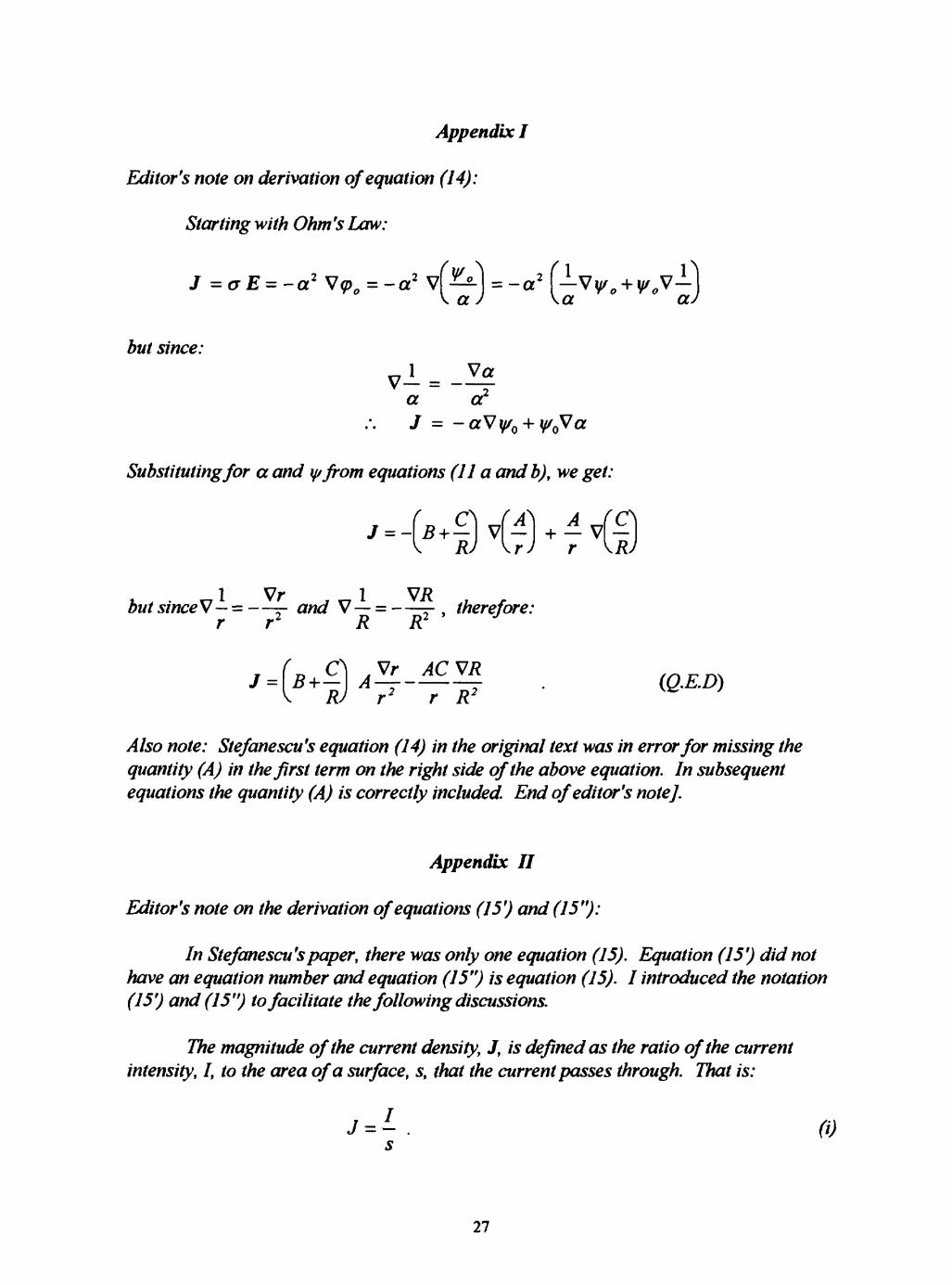
Starting with Ohm's Law:

1J =crE = -a2 V<p=-a2 VM^ = -a2 \-a) \a a

but since:

a a2 J = -

Substituting for a and yfrom equations (11 a and b), we get:

1 Vr 1 VRbut sinceV = =- and V = r-, therefore:

r r 2 R R2 J

r R2(Q.E.U)^ '

Also note: Stefanescu's equation (14) in the original text was in error for missing the quantity (A) in the first term on the right side of the above equation. In subsequent equations the quantity (A) is correctly included. End of editor's note].

Appendix II

Editor's note on the derivation of equations (15') and (15"):

In Stefanescu's paper, there was only one equation (15). Equation (15') did not have an equation number and equation (15") is equation (15). I introduced the notation (15') and (15") to facilitate the following discussions.

The magnitude of the current density, J, is defined as the ratio of the current intensity, I, to the area of a surface, s, that the current passes through. That is:

J = ~. 0) s

27

The portion of current, dl, that crosses an elemental-area, ds, is given by:

A

dl = J.ds = (J.r)ds = JdscosB (ii)

where:J = current-density vector,ds = elemental-area vector, defined by the magnitude of the area, ds,

A

and a unit vector, r, perpendicular to it.A

r = unit vector that lies in a direction perpendicular to the elementalA A

area ds. The magnitude of r equals unity (\ r \ 1)A

6 = angle between the vectors J and r.

Equation (ii) shows that the portion of the current intensity, dl, that crosses the elemental-area, ds, is a function of the angle 6. At 6 = 0 degrees, all the current goes through the elemental-area, ds, and at 6 = 90 degrees, none of the current goes through,

A A

because r will be perpendicular to J andJ. r = 0 (which also means that the elemental- area, ds, will be parallel to J).

If the elemental-area, ds, represents an element of the surface of a sphere, of radius R, that surrounds the a center, such that the location of the a center coincides with the center of the sphere, then the elemental-area ds can be expressed by :

ds = R2 dQ. (Hi)

whereR = radius of the sphere, andf/Q = solid angle subtended from the center of the sphere to the elemental-area,

ds.

Substituting, R2 dQ., for ds, in equation (ii), we get:

dI = (J.r)R2 dfl. (iv)

A

In equation (15'), Stefanescu used the VR instead of the unit vector, r, in the above dot-product expression, and he wrote:

dl = (J.VR) R2 dfl (v)

Before proceeding any farther, we will show that his notation is correct and thatA

the gradient ofR, P/?, /5 equal to the unit vector, r.

28

A position vector R, which represents the radius of the sphere surrounding the a center, may be expressed in terms ofx, y, z and the unit vectors i,j, k (along the x, y, z directions, respectively) as:

R=xi+yj +zk, (vi)

A

or, it also may be expressed in terms of its magnitude, R, and a unit vector, r, along the direction ofR, so that:

R=Rr (vii)

From equations (vii) and (vi), we can write:

A R x i+y j+z kr = = £_£ R R

The magnitude ofR, is given by:

thus, differentiating equation (ix), with respect to x, y, andz, we get:

= 2x = ~ 2 V*2 +y2 +22 ~ R

2z

and therefore,

Comparing equations (viii) and (xii) we can see that:

R = \R\ = yx2 +y2 +z2 , (ix)

and the gradient ofR, PR, is defined by:

^ D . dR . dR , . . VR = i + j + k , (x)

dx dy J dz

dR 2y y , .. J = = ±- (xi)

V7r> x y z i x i+y j+z k . ...VR = i+ j + k = ̂-^ (xii)R R R R V

29

P/? = r (Q.E.D.) (xiii)

Now we continue with the derivation of Stefanescu's equations (15') and (15").

Substituting for Jfrom equation (14) into equation (v), we get:

RJ r 2 r R

A+ CR)A^-± ' r r

(15')

From equation (15'), we can see that as R tends to 0, the first term tends to zero. Furthermore, as shown in Figure 1 (seepage 15), the distance, r (from the point electrode at O to the measuring point atM) tends to das the distance, R (from the a - center at S to the measuring point at M) tends to zero. Therefore, as R tends to zero, equation (15') reduces to:

r A i dl = \ ~-C (VR)2 \ da. (xiv)

Let us re-examine the gradient ofR:

As shown in equation (xii),

R R R (xv)- x * + y J +z ^ _ _

The dot product P/f . P/f is equal to 1 (because Li =1 and Lj = 0, Lk = 0, etc.) and thus:

= VR.VR =

Therefore, equation (xiv) reduces to

dl = - d

Integrating both sides of the above equation, we get

30

AC r

77»w completes the derivation of equations (15') and (15"). End of editor's note.]

Appendix III

[Editor's note on equation simplification:

In the original equation there is a typesetting error in a subscript ofR and the term (Pr. PR2) should be (Vr. PRt), as it is given below.

The equation

[dl =] (j.VR^Rf

D2dQ.

+D2

is simplified as follows:

(1) as shown earlier (PR)2 = / (see equation (xvi) in appendix II), and therefore the (PR)2 terms in the bracketsare set to unity,

(2) the terms with Rj2 , in the brackets, are set to zero.(3) the terms with Dj/Rj andCj/Rj , in the parentheses, cancel (after the above

simplifications) as shown below:

r R} R2 J l 1J ^ R,

r l { R J R, R-,

r R

end of editor's note].

I] R

31

8 9 10 11

Plate 1. [Editor'snote:The following plate caption was added by this editor because one was not

provided in the original article. The above diagram was scanned (from a somewhat distorted Xerox copy of the original), then it was edited and annotated. The letters P, Q, 8], and 82,' the axes labels and tick-mark values; and the horizontal and vertical lines through Sj and 82; were added to original diagram.]

Diagram showing equipotential contours (solid lines) and equal- conductivity contours (dashed lines) in a vertical cross section that passes through two a centers, Si and S2, located at (x, z) coordinates of (0,2) and (3,6), respectively. + oo and - <x> symbols represent the electrical potential at current electrodes P and Q, which are located at (x, z) coordinates of (-4,0) and (11,0), respectively. The vertical dashed line (at x = 3.5) passes through the mid point between the electrodes P and Q and represents the zero-equipotential line in a homogeneous half space (with no a centers). Note deflection of zero- equipotential line (to the right of the vertical dashed line) in response to the presence of the two a centers.

32