U.S. Congressional Vote Empirics: A Discrete Choice

Model of Voting

Kyle Kretschman

The University of Texas – Austin

kyle.kretschman@mail.utexas.edu

Nick Mastronardi

United States Air Force Academy

nickmastronardi@gmail.com

February 15, 2010

Abstract

This paper uses United States congressional district level data to identify how in-

cumbency, candidate campaign expenditures and district voter registration character-

istics influence final vote shares. We estimate the factor impacts using a representative

agent-based discrete choice model and an estimation method similar to Berry, Levi-

sohn, and Pakes (1995). District-level partisan voter registration statistics provide the

observable distribution of voter heterogeneity, therefore, it is not necessary to estimate

the voter heterogeneity distribution parameters. This allows for the parameters to

be estimated with precision even though there are a relatively small number of ob-

servations. Moreover, the structural discrete demand model with voter heterogeneity

provides a general methodology of factor impact estimates by which we can formally

test the modeling restrictions found in Levitt (1995) and Gerber (1998).

1

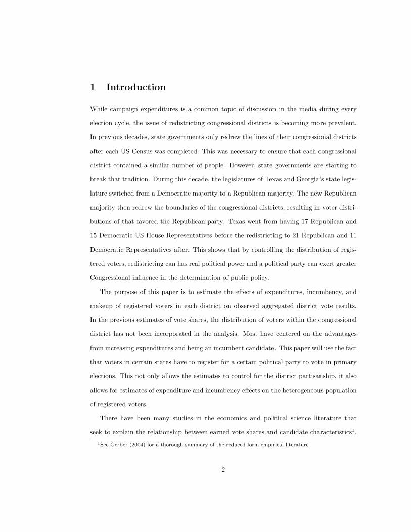
1 Introduction

While campaign expenditures is a common topic of discussion in the media during every

election cycle, the issue of redistricting congressional districts is becoming more prevalent.

In previous decades, state governments only redrew the lines of their congressional districts

after each US Census was completed. This was necessary to ensure that each congressional

district contained a similar number of people. However, state governments are starting to

break that tradition. During this decade, the legislatures of Texas and Georgia’s state legis-

lature switched from a Democratic majority to a Republican majority. The new Republican

majority then redrew the boundaries of the congressional districts, resulting in voter distri-

butions of that favored the Republican party. Texas went from having 17 Republican and

15 Democratic US House Representatives before the redistricting to 21 Republican and 11

Democratic Representatives after. This shows that by controlling the distribution of regis-

tered voters, redistricting can has real political power and a political party can exert greater

Congressional influence in the determination of public policy.

The purpose of this paper is to estimate the effects of expenditures, incumbency, and

makeup of registered voters in each district on observed aggregated district vote results.

In the previous estimates of vote shares, the distribution of voters within the congressional

district has not been incorporated in the analysis. Most have centered on the advantages

from increasing expenditures and being an incumbent candidate. This paper will use the fact

that voters in certain states have to register for a certain political party to vote in primary

elections. This not only allows the estimates to control for the district partisanship, it also

allows for estimates of expenditure and incumbency effects on the heterogeneous population

of registered voters.

There have been many studies in the economics and political science literature that

seek to explain the relationship between earned vote shares and candidate characteristics1.

1See Gerber (2004) for a thorough summary of the reduced form empirical literature.

2

Gerber (1998) and Levitt (1994) both estimate electoral factor impacts using reduced-form

models. They differ in their techniques to control for the endogeneity that final vote shares

and candidate expenditures may be co-caused by a factor such as candidate quality. An

eloquent or charismatic candidate may garner more supporters, more votes, more financial

support, and have larger expenditures. Gerber employs 2 Stage Least Squares and tries

several instruments. Levitt introduces the unobserved qualitative regressor, but then uses

repeat electoral races to difference it out and obtain consistent estimates.

Berry, Levinsohn, and Pakes (1995) (hereafter BLP) introduce a structural discrete choice

demand model which has been employed across many industries to estimate the impacts

of product characteristics using observed product market share. In this paper, we apply

their methodology to explain the impact of candidate characteristics on observed candidate

vote share received. We modify the discrete product-demand estimation methodology from

BLP for observed aggregate vote share data. In our model, the market is a congressional

district, the products are the candidates seeking elections, the characteristics are incumbency

status and expenditures, the market share is the vote share and the consumer heterogeneity

random-coefficient distribution is the partisan voter registration distribution.

This paper contributes to the campaign expenditure literature in two ways. First, the

discrete distribution of district partisan voter registration statistics are introduced into the

BLP model to account for voter heterogeneity. Rekkas (2007) is the first and only paper

until this one to apply the BLP methodology to election data. She analyzes the 1997

Canadian Parliamentary Election. She uses the same methodology used in BLP. The main

differences between our work is that she did not have voter registration statistics and thus

had to estimate parameters of the random-coefficient heterogeneity distribution, and we are

analyzing many years of US House of Representative elections in the United States. The

major drawback of Rekkas (2007) is that the Canadian elections are generally multi-party,

which requires estimating more parameters in an already parameter-heavy framework. This

3

leads to very imprecise estimates of the parameters in the full model. Fortunately, our data

have allowed us to achieve a high degree of accuracy because we do not need to estimate the

population distributions. In fact, the observed voter registration data provides an additional

source of variation that improves the precision of our estimates.

The second major contribution of this paper is that the earlier reduced form studies of

Levitt (1994) and Gerber (1998) are special cases of our structural model. Levitt (1994)

introduced the unobserved candidate regressor and our model also includes this regressor.

However, instead of differencing the equations to remove this regressor, our method explicitly

solves for this unobserved regressor. We then use instruments similar to Gerber (1998) to

deal with the endogeneity between the unobserved regressor and the candidate’s expenditure.

The main difference between our work and these two studies is that we estimate a structural

model instead of positing a reduced form. In fact, the Levitt and Gerber models are specific

cases of our model. Both studies implicitly imply that there is no heterogeneity in the voter

population. Therefore, we empirically test the set of parameter restrictions on our model

that yield the Levitt (1994) and Gerber (1998)regressions. We show that the voters who are

registered to different parties respond differently to the candidate characteristics.

The organization for the remainder of this paper is as follows. Section 2 presents the

discrete choice demand model of voting and provides the general estimation equation. It

further introduces the voter registration distribution as the random-coefficient distribution,

and briefly explains how to estimate the parameters using observed vote shares. Section

3 explains the data used for this analysis. Section 4 provides and interprets the empirical

results. Then we compare our results with the previous literature and test the equating

restrictions. Section 5 concludes.

4

2 Discrete Choice Model Specificcation

In this section, as is standard in the discrete choice literature, we derive the probability of

voting for each of the candidates. In our model, there are three different types of represen-

tative agents in every congressional district that each have a random taste shock for both

of the candidates. As will be shown, the mean utility of each candidate and an assumed

distribution for the random tastes will completely determine the probability that each type

of agent votes for each candidate. Then, the predicted market share function for each can-

didate is the average of the three probabilities weighted by the proportion of each type of

agent in the market. Our estimation of the parameters of the model is based on the fact that

there are covariates that are orthogonal to the model error that occurs because candidate

quality is unobserved.

The main difference between our methodology and the previous literature is that we

are able to observe the proportion of each type of agent in each market. This provides us

two main advantages. First, there is no need to estimate the distribution parameters so

the estimation is much more precise. Second and more importantly, we are able estimate

different parameters for the different agents. Instead of having a mean and variance of

the parameter over the distribution, we estimate different mean values for each type of

agent. This provides much more detailed information of how voter utility responds to the

candidate’s characteristics.

2.1 Utility of a Representative Agent

We assume that there are three representative utility-maximizing agents in each district.

One type is a voter who is registered for the Democratic Party, the second type is a voter

registered for the Republican Party, and the third type is a voter who is not registered for

either of those two parties. Each type of agent is facing a discrete voting decision: whether

to vote for the candidate from the Democratic Party, the Republican Party, or not vote for

5

one of the two candidates from the dominant parties. The third option can be considered

the outside option. It includes the choice of voting for a third party candidate. The outside

option is defined this way because, for the past decade, every representative to the US House

has been a member of the Democratic or Republican party2. The voting decision is modeled

as follows:

maxj∈{0,1,N}

Unmj = Vn(pmj , xmj) + enmj (1)

From this point on, the Democratic Party is by the subscript 0, the Republican Party by

the subscript 1, and registered voters who did not pick one of those parties is represented

by the subscript N. For this decision problem, the j subscript denotes the different voting

options: Democratic, Republican, and Neither. The m subscript denotes the market which

is defined as a congressional district and the n subscript denotes the three different types of

agents. For example, U0m1 is the utility that a registered Democrat in congressional district

m receives from voting for the Republican candidate. It is important to note that this utility

function is defined as the utility of voting for a specific candidate and not the utility from

having that candidate be your representative3.

The pmj variable is the campaign expenditures by candidates j in market m, and xmj

is a vector of observable candidate and market characteristics. We define xmj as the vector

of control variables (Incumbent, Senate Race, Presidential Race, Democratic Party Dummy

Variable, State Dummy Variables, and a Constant)’. Therefore, Vn(·) is the indirect utility

from all of the observable characteristics and enmj is the unobserved utility that equates Vn(·)

and the actual utility of each individual. We assume that Vn(·) is linear in its arguments.

There are two sources of unobserved utility. The first is the utility from the candidate

2While Rekkas (2007) includes all the minor parties when analyzing Canadian elections, Lee (2008) makes

the same outside option assumption that we do since the United States government is completely dominated

by the two major parties.3This distinction is discussed more in the extensions.

6

characteristics that are observed by the representative agent but unobserved by the econo-

metrician, denoted by ξmj . These unobserved candidate characteristics are different for each

candidate in each market but the same across the different agents within a market. Hence,

there is no “n” subscript since the utility does not vary by agent. The second source of

unobserved utility is the idiosyncratic utility shock, denoted by εnmj . This shock represents

the unobserved “taste” for each candidate that varies by agent. Therefore, enj = ξmj + εnmj

and we rewrite equation 1 as:

Unmj = αnln(pmj) + βnxmj + (ξmj + εnmj) (2)

2.2 Probability of Voting

While Unmj is not observable, using the fact that each agent is a utility maximizer and

assuming a distribution on εnmj allows us to derive the probability that each type of agent

will vote for each of the candidates. First, define the mean utility level for each candidate

in each market as:

δnmj ≡ αnln(pmj) + βnxmj + ξmj (3)

∴ Equation 2 is simplified to Unmj = δnmj + εnmj (4)

Simplifying the utility this way shows that the δnmj and the individual shock completely

determine the voting choice for each individual, thereby completely determining the prob-

ability that the representative agent votes for each candidate. However, note that in each

market m, ξmj is the same for each n. This restriction is necessary to estimate the parame-

ters since we do not observe individual voting choices of the different types of agent. From

here on we will drop the m subscript to make the equations more concise.

Since the outside option does not have any candidate characteristics and a discrete choice

model can only identify relative utility levels, we redefine εnj as utility shock difference

7

with the outside choice shock and normalize δnN ≡ 0. Therefore, within each market, the

probability of the representative agent of each type voting for each candidate can be found

as:

Pnj =

∫Bnj

dP (εnj , εnk) where Bnj = {εnj , εnk|Unj > Unk ∀j 6= k} (5)

∴ Bnj = {(εnj , εnk)|δnj + εnj > 0; δnj + εnj > δnk + εnk} (6)

We assume that all εnj are independently distributed type 1 extreme value, P (εnj) =

exp(−exp(−εnj)). As in standard BLP, the assumptions of the model lead to the well known

result that the predicted probability of each type of agent voting for candidate j has the

logit form4.

Pnj =eδnj

1 +∑

j∈{0,1}eδnj

(7)

2.3 The Discrete Distribution of Agents and Random Coefficients

As indicated above, we are assuming there is a separate utility functions for the three dif-

ferent type of agents. The functional form of utility is the same for each agent, but the

coefficients on the candidate characteristics can differ by agent. Therefore, this is a random-

coefficients utility model similar to BLP. BLP introduces random coefficients into the model

under the argument that different product characteristics can influence heterogeneous con-

sumers differently. This has the dual virtues of being more realistic and alleviating the

substitution pattern restrictions imposed by a standard logit model. The additional pa-

rameters provide explicit information on how candidate characteristics affect the different

registration groups. For example, α10 measures the utility effect (and hence vote share effect)

for a registered Democrat from an increase in expenditure by the Republican candidate.

4See Train (2003) pg. 78 for the algebra

8

Our model relates significantly to the model in Berry, Carnall and Spiller (2006) as

well as to BLP. This is do to the assumption of a discrete distribution of heterogeneous

agents. BLP assume the coefficients are distributed normally and estimate the distribution

parameters for each coefficient. Berry, et al (2006) assume that the there are two discrete

type of agents and estimate the percentage of each type of individual. Unlike Berry, et al

(2006), we observe the percentage of people in each group in each district and therefore do

not have to estimate the percentages for each type of agent or argue that they are identified.

In each market m, let:

µm0 ≡ # of registered Democrats in district

total # of registered voters in market m

µm1 ≡ # of registered Republicans in district

total # of registered voters in market m

µmN ≡ 1− µm0 − µm1

2.4 Predicted Market Share Function

The probability that an agent of type n will vote for j and the proportion of each type of

agent in each market are shown in the two previous sections. Combining them, the predicted

vote share function for each candidate is the sum over the probability of each type of agent

voting for candidate j weighted by the proportion of each type of voter.

sj(α, β, ξ;µ) =∑

n∈{0,1,N}

µn ∗eδnj

1 +∑

j∈{0,1}eδnj

(8)

2.5 Elasticities of Expenditure

The advantage of having the observed heterogeneity in the model is highlighted by the own

and cross elasticities of expenditure. These explicitly elasticities show the how a percentage

increase in expenditure will change the percentage of each type of agent that votes for him.

9

Define η∗jj as the own expenditure elasticity. This is the percentage change in vote share for

candidate j if he increases his expenditure by 1%. In our model:

η∗jj =∂s∗j (α, β, ξ;µ)

∂pj

pjs∗j (α, β, ξ;µ)

=

∑n∈{0,1,N}

αn ∗ µn ∗ eδnj

1+∑

j∈{0,1}eδnj

[1− eδnj

1+∑

j∈{0,1}eδnj

]s∗j (α, β, ξ;µ)

(9)

The numerator of equation (9) shows that the overall change in vote share is the sum of

the change in vote share from each type of agent. Therefore, our model provides a closed

form answer for the change in voting behavior for each type of agent.

Similarly, define η∗jk as the cross expenditure elasticity. This is the percentage change in

vote share for candidate j from a 1% increase in expenditure by candidate k.

η∗jk =∂s∗(α, β, ξ;µ)

∂pk

pks∗j (α, β, ξ;µ)

=

−∑

n∈{0,1,N}αn ∗ µn ∗ eδnj

1+∑

j∈{0,1}eδnj

eδnk

1+∑

j∈{0,1}eδnj

s∗j (α, β, ξ;µ)(10)

2.6 Endogeneity of Unobserved Candidate Characteristics

ξmj is defined as all the characteristics of the candidate that are unobserved by the econome-

trician but which affect the mean utility level of the candidate. Some of these characteristics

are charisma, public speaking ability, physical appearance and performance in office for in-

cumbents. These characteristics not only affect the number of votes a candidate receives,

but they potentially affect the amount of contributions a candidate raises. Furthermore,

a candidate with greater contributions can expend more on the congressional race. With-

out controlling for any other factors other than incumbency, this causes the unobserved

10

characteristics to be endogenous to the candidate’s expenditure.5

However, our model controls the distribution of partisan voter in each district. Con-

trolling for district partisan registration statistics in Congressional races may explain any

indirect causation that biases the previous expenditure impact estimates. The voter regis-

tration statistics in each district are continuously changing. In fact, a lot of the candidate

expenditure during each election is focused on registering people to vote and concurrently

convincing people to register for the candidates party. If the unobserved candidate char-

acteristics induce a person to register for that candidates party in a similar way that they

induce a person to vote for the candidate, the registration statistics could capture some of the

correlation between expenditures and the unobserved candidate characteristics. Therefore,

controlling for the voter distribution in each district provides additional controls that may

limit the endogeneity of expenditures.6Unfortunately, we are unable to statically test this

claim using the standard Hausman test due to computational limitations. The estimation

methods are highly nonlinear and take many hours to run so it would take many months to

construct the Hausman statistic. In light of this fact, we will estimate the model ignoring

endogeneity and also estimate it controlling for the presence of endogeneity.

2.7 Estimation

2.7.1 Estimation Ignoring Endogeity

If we ignore the endogeneity of expenditure and the unobserved candidate characteristics,

we can ignore the presence of the unobserved candidate characteristics and estimate the

5The instruments we use will be discussed in the data section.6This argument will be strengthened once we are able to gather data on each candidates gender, age, and

race and include those variables in the estimation. This data gathering is currently happening.

11

model using nonlinear least squares. The estimation equation is:

(α, β) = minα,β

1

2M

M∑m=1

∑j∈{0,1}

smj − ∑n∈{0,1,N}

µmn ∗eδmnj

1 +∑

j∈{0,1}eδmnj

2

(11)

with δnmj ≡ αnln(pmj) + βnxmj

This estimation method picks the vector (α, β) so that the sum of square differences

between the observed vote share and the predicted vote share for each candidate in each dis-

trict is as small as possible. Robust standard errors are then calculated following Wooldridge

(2002).

2.7.2 Estimation Controlling for Endogeneity

Since the estimation of this type of model is discussed extensively in BLP and in many

other sources, we provide only a brief summary of the process. The endogeneity of the

unobserved characteristics provides the standard instrumental variables moment conditions

for the model, E(Z ′ξ) = 0. Z is a vector of exogenous covariates, including instruments for

the endogenous expenditure regressors and ξ is the vector of unobservable characteristics for

all the candidates. The main result from Berry (1994) is that for each vector of parameters

(α, β), there exist a unique vector ξ that equates the predicted vote share function with

the observed vote shares, s = sj(α, β, ξ;µ), in every market. This means that ξ is a highly

nonlinear function of (α, β; s, µ), where s is the vector of observed market shares. The ξj

for each candidate can be found market by market for each candidate using a contraction

mapping similar to BLP7. Therefore, the estimation of (α, β) reduces to a standard GMM

objective function.8

7Mike Carnall graciously provided an outline of how to program this contraction mapping with discrete

heterogeneity. Also, Dube et al (2009) provides great guidance on practical problems of this estimation

technique.8Our problem is computationally much simpler than BLP because it does not require any simulation of

integrals to estimate the coefficient distribution parameters. A copy of the Matlab code used to estimate

12

(α, β) = minα,β

[Z ′ξ(α, β; s, µ)]′[Z ′Z]−1[Z ′ξ(α, β; s, µ)] (12)

The standard errors for this are calculated using the delta method.9

3 Data

3.1 Overview

Our data set consists of US Congressional district-level voter registration statistics by party,

the party of incumbency and candidate expenditures for the 2002, 2004, 2006 and 2008

Congressional House elections. The data set was compiled from different sources. The

voter registration statistics and final vote counts were collected from the each state’s Board

of Elections. Some states provide this information on their website and some had to be

contacted for the information. All of the incumbency and expenditure data come from the

Federal Election Commission.

There are 30 “states”10 that require voters to register for a specific party if they want

to vote in the primary elections. These states are said to have “closed primaries”. We

do not include states that have “open primaries” because they either do not ask for party

affiliation on their voter registration forms or the chosen party has no implications for their

voting options. Therefore, the states with “open primaries” do not provide a reliable report

of the voter registration statistics. Of the 30 states with “closed primaries”, we were able

to assemble data from from the Congressional districts in 26 states. The majority of these

districts have voter registration data available for all four elections this decade11. We limit

our model is available upon request.9We do not need to correct for measurement error in our standard errors since the observed vote shares

are calculated using the actual number of votes received.1029 states plus the District of Columbia11The data for districts in Kansas and Utah is only available from 2008 and Connecticut does not have

the information for 2006.

13

the data to the elections this decade because the number of Congressional districts per state

is reallocated after every census. For example, there are Congressional district from the

2000 election that were erased for the 2002 election and vice versa. Also, we do not employ

data on districts from states that that lack the voter registration statistics aggregated at

the congressional district level. The data for the missing districts could conceivably be

aggregated by contacting each individual voting precinct in each congressional district, but

this would require contacting thousands of different precincts across many states and lies

beyond the scope of our study.

The theoretical model is designed to analyze the districts where individuals have the

choice between voting for a Republican candidate or a Democratic candidate. This leads

us to include only districts in which both a Republican and a Democratic candidate ran for

the office and spent more than $10,000 each and to exclude districts where any additional

candidates ran and spent more than $10,000. As mentioned earlier, this restriction is based

on the fact that every member of the US House of Representatives is either a Republican or

a Democratic. In the US, the two parties completely dominate the federal government and

voting for a candidate outside of these two parties is similar to not voting.

Given these restrictions, our sample observation size is 478 congressional districts. With

2 candidates in each district, this yields 956 different observations12. For example, the 2nd

Congressional district in California during the 2002 election is one district with 2 observa-

tions, while the 2nd Congressional district in California during the 2004 election is another

district with 2 different observations. The summary statistics for the congressional districts

is provided in the Table 1. All expenditure data is in 2008 dollars.

The summary statistics show that, on average, about 77% of the registered voters in our

districts are partisan to either the Democratic Party or the Republican Party and that a

12This sample size will be reduced in the instrumental variables estimation because some of our instruments

are lagged values.

14

Table 1:

Summary Statistics of Congressional Districts

Variable Full Sample Restricted Sample

Mean St. Dev. Mean St. Dev.

Pct. Registered Democrat .4494 .1382 .4082 .1133

Pct. Registered Republican .3326 .1226 .3652 .0990

Pct. Democrat Incumbent .44744 - .3808 -

Pct. Republican Incumbent .4322 - .4979 -

Democratic Expenditure 905,247 973,043 1,057,618 1,066,246

Republican Expenditure 855,201 1,042,171 1,136,768 1,130,382

Democratic Vote Share .2946 .1511 .3058 .1122

Republican Vote Share .2524 .1500 .2964 .1099

Districts 782 478

great deal of money is being spent in an attempt get elected. Candidates from both parties’

average over a $1,000,000 in campaign expenditures. There is a very high variance on the

amount spent, but overall these elections consume a large amount of financial resources.

Last, the vote shares are calculated by dividing the number of votes received by the total

number of registered voters in the district. Both parties average about a 30% vote share,

which corresponds to a 60% voter turnout rate, which is fairly typical in the US.

Table 1 provides summary statistics for the full sample of 738 districts along with the

restricted sample that will be used for estimation. There is no statistical difference between

the two samples along these dimensions, however the average expenditure measure is larger

in the restricted sample because one of the restrictions involves removing districts having low

expenditure by one of the candidates. Along with higher expenditures, the data restrictions

15

cause the difference between Pct. Registered Democrats and Republicans to be smaller. The

averages in the restricted sample are only 4% different, whereas they were 11% different in

the full sample. The higher expenditures and lesser difference in registered voters show that

the the restricted districts are much more likely to have competitive races. As argued in

Erickson & Pelrey (2000), this leads to much better estimates of the effect of expenditures

on Congressional outcomes.

3.2 Instruments

For a valid instrument in this situation, we need a regressor that is correlated with the

candidate’s expenditure but uncorrelated with the number of votes that candidate received in

the election. Here we exploit the iterative nature of elections and the fact that Congressional

district boundaries provide a clear distinction for each market. United States congressional

elections occur every two years. Therefore, we can use characteristics of lagged elections

and characteristics of Congressional districts within the the same state to instrument for

candidate expenditure.

Since we need to identify coefficients for three different types of agents, we need three

different instruments. We start by adapting the same two instruments that Rekkas (2007)

used. The first instrument is the total expenditures by the Democratic candidate and the

Republican candidate from the previous election. This instrument was first used by Gerber

(1998) in his study of Senate elections. The second instrument is a measure of how close the

previous election was in each district. This instrument can be interpreted as the historical

competitiveness of the election for each district. It is defined as the absolute value of the

difference in percentage of votes received by the Democratic and Republican candidates.

16

Therefore, the closeness measure ranges from 0 to 1, where the values near zero are districts

where the previous election results were very close and the values near 1 are where the

previous election results were landslides. The third instrument is the average expenditure of

all the candidates in the same state during the same election. Since state and congressional

district boundaries are clearly defined, this instrument uses information from the districts

that are related by being part of the same state13.

The use of lagged total expenditure as an instrument, a la Gerber (1998) and Rekkas

(2007), is less obvious in our environment. The main issue with using the lagged total

expenditure is that congressional elections in the United States are different from the Senate

elections that Gerber studied and Canadian parliamentary elections Rekkas studied. Senate

elections only occur every six years and Canadian elections occur every four years. In

their cases, it is easy to assert that previous election expenditures are uncorrelated with

the current campaign elections. Both authors argue that lagged total expenditure is valid

because they use the total expenditure instead of just the previous candidates expenditure

and there is very large turnover between incumbents and challengers. This characteristic

is not as straightforward for US congressional elections. However, unlike Gerber (1998)

and Rekkas (2007), we are able to make use of the voter registration statistics of each

district. Since these statistics change over time, the voter registration statistics act partially

as a summary of past candidate expenditures. Since a lot of campaign expenditure is

concentrated on registering voters to their party, the correlation between lagged expenditure

and current expenditure can be captured in the registration statistics. This fact, combined

with the use of total lagged expenditure instead of individual candidate’s lagged expenditure,

13See Appendix A for the reduced form regressions of candidate expenditure on the instruments.

17

makes it a valid instrument.

4 Empirical Results

The results of three different specifications of the theoretical model are presented in Tables

2 and 3. Both tables show three different specifications of the model. The first column does

not interact expenditure with any other variables. The second column interacts expenditures

with the incumbency dummy variable to estimate the differing effects of spending by incum-

bents and challengers. The third column interacts expenditure with the Democratic party

dummy variable. This allows us to differentiate the effect of spending by the Democratic

candidates and the Republican candidates. Specifically, it allows us to estimate of the effect

that expenditure by the Democrat has on registered Democrats, Republicans and nonpar-

tisans. The same holds true for expenditure by a Republican candidate.14. One surprising

result from Rekkas(2007) was that the variance of the expenditure coefficient distribution

was larger than the mean, which implies that not all voters have a positive marginal util-

ity for expenditure. As will be shown, our results confirm this fact and show that it is a

result of registered Democrats reacting negatively to Republican candidates and registered

Republicans reacting negatively to Democrat candidates.

As mentioned earlier in the paper, the following tables show the coefficient results from

two different estimation methods. All specifications also include dummy variables for the

State of each district, but these coefficients were omitted since they are not of interest.

The first table presents estimation results when it is assumed that the unobserved product

14We only allow for random coefficients on the expenditure covariate at this time because we need to

identify more instruments before allowing random coefficients on Incumbency and dDem

18

characteristics are uncorrelated with any of the regressors. In the this situation, there is no

endogeneity bias by ignoring these unobserved characteristics so the model can be estimated

using Nonlinear Least Squares (NLS) and the resulting coefficients are reported in Table

2. The second table presents the estimation results when we control for the endogeneity

of the unobserved product characteristics. The estimation is done using the BLP GMM

methodology. Each estimation also reports one or two Wald statistics that test if the random

coefficients are equal statistically different. These tests are discussed in the subsection 4.3.

The last section presents the average elasticities predicted by these results and breaks the

elasticities into agent specific elasticities.

4.1 Model without Endogeneity

Before examining the the random coefficients on expenditures, first look at the the coefficient

results for the other control variables. Care must be given when interpreting these coefficients

since they are not coefficients from a linear model. These coefficients can be interpreted in

an analogous manner to a standard logit regression. The Senate Race, Presidential Race,

and Constant regressors are the same across the two candidates so they will only effect

the probability of voting. The coefficient terms support the argument that a person is

predisposed not to vote because there is a time cost to voting. The Constants are all

negative and this means that without any other factors, an individual would be likely not

to vote. If all other factors were equal to zero, the negative constant value of -1.65 implies

that each type of agent would have a 14% probability of voting. This substantiates the idea

that there is implicit cost of voting. Without other factors, a person is unlikely to take the

time to vote.

19

Table 2:

NLS Parameter EstimatesVARIABLES (1) (2) (3)

(µ0)ln(expend) 0.1793*** 0.07122*** 0.0018(0.0123) (0.0298) (0.0324)

(µ1)ln(expend) 0.1348*** 0.2224*** 0.2438***(0.0136) (0.0235) (0.0203)

(µN )ln(expend) 0.1358*** 0.1697*** 0.1114***(0.0146) (0.0215) (0.0227)

(µ0)ln(expend)*Incumb -0.0802***(0.0344)

(µ1)ln(expend)*Incumb -0.2749***(0.0326)

(µN )ln(expend)*Incumb -0.1702***(0.0250)

(µ0)ln(expend)*dDem 0.1805***(0.0378)

(µ1)ln(expend)*dDem -0.2001***(0.0425)

(µN )ln(expend)*dDem 0.0783***(0.0293)

Incumbent 0.2603*** 1.1086*** 0.2702***(0.0027) (0.0024) (0.0027)

dDem 0.0554*** 0.0401*** 0.0179***(0.0004) (0.0004) (0.0004)

Senate Race -0.0172*** -0.0128*** -0.0313(0.0021) (0.0020) (0.0020)

Presidential Race 0.7882*** 0.7890*** 0.7974***(0.0014) (0.7890) (0.0014)

Constant -1.6542*** -1.6528*** -1.4696***(0.0739) (0.0652) (0.0760)

Observations 956 956 956R2 0.80 0.83 0.81Wald Tests:χ2ln(expend) = 5.8871 10.154 25.811

Prob = 0.9473 0.9938 1.0000χ2ln(expend)∗Interaction = 9.188 28.8906

Prob = 0.9899 1.0000Robust standard errors in parentheses

*** p<0.01, ** p<0.05, * p<0.1

Note: Coefficients for the state fixed effects are omitted.

20

The positive coefficients on Presidential Race show that a person is more likely to vote

in the Congressional elections when they can also a Presidential election at the same time.

The estimate is very consistent throughout the specifications and the estimate implies a

marginal effect of about 9%. A little surprising the result that the Senate Race coefficient

is significantly negative. This implies that voters are less likely to vote in a Congressional

election when a Senate Race is running concurrently. However, the coefficients are all very

small, with a marginal effect of -.3%, and therefore this has very little impact. A concurrent

Presidential election increases the probability of voting much more than a concurrent Senate

race decrease the probability. Overall, these effects fit within standard theories of voting.

The Incumbent and Democratic dummy variable regressors do vary by candidate and

therefore effect the choice of who to vote for. The dDem coefficients are all positive but very

small. The estimates imply that a Democratic candidate has about .25% advantage in vote

share. However, an Incumbent has a substantial intrinsic advantage. The first and third

columns, without the expenditure Incumbency advantage, both estimate that an incumbent

has about a 3% point advantage in an election. This estimate corresponds exactly with the

prior estimates by Levitt (1994). The second column implies an advantage of 13%. This

seems very high in that and we believe this is a result of not controlling for Incumbent

performance while in office that is included in the unobserved candidate characteristics.

Now, lets look at the random expenditure coefficients and how to interpret them. The

first specification does not interact the expenditure term and therefore the coefficient on

(µ0)ln(expend) is the average marginal effect of expenditure on a registered Democrat. In

the second specification, ln(expend) is interacted with the Incumbency dummy variable, so

(µ0)ln(expend) is now the average marginal effect of expenditure on a registered Democrat

21

by a non incumbent candidate. The average marginal effect of an incumbent candidate on

a registered Democrat is the sum of (µ0)ln(expend) and (µ0)ln(expend)*Incumb. Finally,

the third specification interacts expenditure with the Democratic party dummy variable.

(µ0)ln(expend) is now the average marginal effect of expenditure on a registered Democrat

by a Republican candidate. The average marginal effect of Democratic candidate on a

registered Democrat is the sum of (µ0)ln(expend) and (µ0)ln(expend)*dDem. Similarly to

the (µ0) coefficients, the (µ1)ln(expend) coefficients are the effect on a registered Republican

and the (µN )ln(expend) coefficients are the effect on a nonpartisan registered voter.

The signs of the coefficients are across all the specifications are as expected. In the

second specification, the results are a little surprising that all the effects of incumbent

expenditure are estimated to be negative which implies an incumbent loses vote share by

expending more. However, all these coefficients are not significantly different from zero and

this in line with previous estimates of incumbency effects. The first specification shows

that all types of registered voters will respond to an increase in expenditure. The third

specification then breaks this result down and shows that different types of agents respond

very differently to the two types of candidates. The estimates show that a Democrat has zero

(0.00018 but insignificant) marginal response to expenditure by a Republican but a relatively

large response to the expenditure by a Democratic candidate. 15 Conversely, a registered

Republican has a very large marginal response to expenditure by a Republican (0.2438)

but a relatively small response to expenditure by a Democratic candidate (0.2438 + -0.2001

= 0.437). Lastly, the estimate results show that expenditure by either candidate increase

15The magnitude and effects of these coefficients will be discussed in a more intuitive way in the elasticity

subsection.

22

the probability that at non partisan voter will vote for him, with a higher responsiveness

occurring for the Democratic candidate.

4.2 Model with Endogeneity

The BLP model is estimated using lagged total expenditure, average expenditure per can-

didate in the rest of the state and lagged closeness as instruments, and the results are

presented in 3. The coefficient estimates for the nonexpenditure control variables are all

very similar to the the NLS estimates except for Incumbency dummy variable in the second

specification. The magnitude and marginal effect are now in line with the rest of the spec-

ifications however this specification is the least precisely estimated of all six specifications.

This provides an indication that Congressional performance while in office is a very impor-

tant unobserved candidate characteristic. While the estimates for non incumbents remain

precise, the Incumbent estimates are have very high standard errors.

While the estimates on the control variables are all similar to the NLS results, the

estimates on the expenditure coefficients change dramatically. In the first specification, the

NLS results all had similar, positive average marginal effects. The BLP results show that

non partisans are not affected on the margin, while registered Republicans have a much

higher responsiveness than registered Democrats. The second specification implies that a

non incumbent can gain more Republican votes but loses Democratic and non partisan

votes with an increase in expenditure. However, the imprecision in these estimates make

this second specification difficult to interpret. Finally, the third specification provides results

that are very similar to the NLS results. A Republican candidate can increase the chance

a registered Republican and non partisan votes for him while decreases the the chance a

23

Table 3:

BLP Parameter EstimatesVARIABLES (1) (2) (3)

(µ0)ln(expend) 0.1296*** -0.2322*** -0.1444**(0.0418) (0.0147) (0.0692)

(µ1)ln(expend) 0.3224*** 1.0129*** 0.2713***(0.0644) (0.1177) (0.0779)

(µN )ln(expend) 0.0426 -0.3327*** 0.1994***(0.1033) (0.0120) (0.0407)

(µ0)ln(expend)*Incumb 0.4898***(0.1422)

(µ1)ln(expend)*Incumb -0.5541(0.4385)

(µN )ln(expend)*Incumb 0.1542(1.0216)

(µ0)ln(expend)*dDem 0.3509***(0.0709)

(µ1)ln(expend)*dDem -0.0888(0.3208)

(µN )ln(expend)*dDem -1.8176***(0.2238)

Incumbent 0.2013** 0.2462 0.3255***(0.0128) (0.7948) (0.0388)

dDem 0.1457*** -0.0789* 0.2899***(0.0248) (0.0440) (0.0882)

Senate Race -0.0285* 0.0236 -0.0219(0.0162) (0.0191) (0.0885)

Presidential Race 0.8244*** 1.2099*** 0.8147***(0.0464) (0.0723) (0.054)

Constant -1.7448*** -2.3741*** -1.6220***(0.3075) (0.1093) (0.1529)

Observations 728 728 728Wald Tests:χ2ln(expend) = 4.3446 277.77 21.844

Prob = 0.8861 1 1χ2ln(expend)∗Interaction = 58.072 3949.5

Prob = 1 1Robust standard errors in parentheses

*** p<0.01, ** p<0.05, * p<0.1

Note: Coefficients for the state fixed effects are omitted.

24

Democrat votes for him by expending more. However, these results say that a Democratic

candidate will increase positively effect both registered Democrats and Republicans, but

greatly reduce the the probability a registered non partisan will vote for him. The magnitude

of the (µN )ln(expend)*dDem coefficient is very large and more research is needed to explain

this16.

4.3 Testing the Random Coefficients

All previous literature except for Rekkas(2007) is actually a reduced form of our model.

The estimates implicitly assumed that expenditure affected the all voters in the same

way. We explicitly model the heterogeneity and therefore are able to test this assump-

tion. The Wald test statistic at the bottom of each column in the results table is a

test of the null hypothesis that the three discrete random coefficient values are equal

to each other. For example, in Table 2, column 2, the first Wald statistic tests H0 :

(µ0)ln(expend) = (µ1)ln(expend) = (µN )ln(expend). The second Wald statistic tests H0 :

(µ0)ln(expend) ∗ Incumb = (µ1)ln(expend) ∗ Incumb = (µN )ln(expend) ∗ Incumb.. The

null hypothesis is rejected at the 10% level in all the specifications except in the BLP speci-

fication without an interaction. However, this test has a p-value of 0.8861. All of these test

provide very strong evidence that the random coefficients are important because different

types of voters respond in very different ways to candidate expenditures, and this is the first

16As stated earlier, the expenditure coefficient results from the BLP estimation are very different from

the NLS estimation and are sometimes counterintuitive. However, the NLS results are able to replicate

the results of previous empirical work without controlling for endogeneity and provide very intuitive results.

Therefore, we are working on an endogeneity test to see if using the observed heterogeneity of voters removes

the endogeneity of candidate expenditures.

25

Table 4:

NLS Elasticities1% Increase in Expenditure by:

Candidate 0 (Democrat) Candidate 1 (Repbublican)

(∆s0) 0.1061 -0.0458

(∆s1) -0.0475 0.1078

(∆sN ) -0.0469 -0.0452Values are the average elasticities from all the districts.

Table 5:

BLP Elasticities1% Increase in Expenditure by:

Candidate 0 (Democrat) Candidate 1 (Repbublican)

(∆s0) 0.1252 -0.0651

(∆s1) -0.0659 0.1265

(∆sN ) -0.0491 -0.0487Values are the average elasticities from all the districts.

paper to precisely estimate the effects.

4.4 Expenditure Elasticities

Magnitude of a marginal increase in expenditure is difficult to interpret through the esti-

mated coefficients. Therefore, Tables 4 and 5 show the average own and cross elasticities

of an increase in expenditure by each candidate. These elasticities were calculated using

specification (1) of each estimation. The values in each table show average percentage in-

crease in vote share for each candidate by if he would increase his expenditure by 1%. The

average expenditure in these elections was about $1,000,000, so 1% is about $10,000. These

tables show that an Democrat or Republican can increase his vote share by about .11%

26

by spending 1% more. There are 400,000 voters on average in each district, so a $10,000

increases gets a candidate 440 more votes. This increase comes from switching voters from

the other candidate and also convincing people who would of otherwise abstained to vote.

5 Conclusion

This is the first paper to use a discrete choice model when the population heterogeneity

is observed. We provide new insights on the effect that candidate characteristics have on

election outcomes and on the response to these characteristics by different groups. Our

results highlight a very important fact that has not been addressed by previous literature:

the distribution of registered voters in each district is key to the election results. This paper

quantifies the fact that registered voters respond to a larger degree to candidates from their

same party. This finding is important result because individual states have the power to

redraw their congressional districts at anytime. When new congressional districts are created

with the intent to favor one party at the expense of the other, this strategy is known as

redistricting. These results quantify the fact that districting can be a very powerful tool in

affecting the outcome of congressional elections. Combined with the relatively low marginal

gains to campaign expenditures, campaign policy reform for congressional elections should

be more focused on ensuring the fair drawing of districts rather than reforming the laws of

campaign expenditures.

27

6 Appendix

A Reduced Form Regression on Expenditures

This table shows that the instruments satisfy the first condition for being valid instru-

ments. The table shows that the instruments are all individually highly correlated with the

ln(expend) covariate controlling for all the other covariates . Then, column 4 shows that

the correlation still exists for each instrument when all the instruments and all the other co-

variates are included in the regression. The signs of most of the correlations are as expected

also. Higher expenditure in the previous election is correlated with higher expenditure in

the current election. Lagged Closeness ranges from 0 to 1 where a value of 0 means the

the prior election was a tie and 1 where one candidate received all the votes. The negative

correlation implies that as the close outcomes of the prior election are correlated with more

expenditure in the current election. The sign of the correlation between ln(restAvg) and

ln(expend) is not as easy to explain. The negative correlation implies that as the larger

average expenditure of candidates from the rest of the state is correlated with lower expen-

diture levels. While this does not have an intuitive explanation, the correlation, and all the

other correlations, are highly significant and that is all that is required to satisfy the first

condition of a valid instrument.

28

Reduced Form Regressions(1) (2) (3) (4)

VARIABLES ln(expend) ln(expend) ln(expend) ln(expend)

ln(Lagged Total Expend) 0.585*** 0.337***(0.0662) (0.0841)

Lagged Closeness -1.714*** -0.906***(0.205) (0.247)

ln(restAvg) -0.660*** -1.317***(0.145) (0.236)

Incumbent 1.544*** 1.539*** 1.507*** 1.569***(0.0857) (0.0869) (0.0818) (0.0849)

dDem 0.188** 0.188** 0.132 0.200**(0.0929) (0.0936) (0.0879) (0.0915)

Presidential Race -0.201** -0.209** -0.0926 -0.532***(0.102) (0.102) (0.0899) (0.119)

Senate Race -0.0341 -0.0453 0.00623 -0.305***(0.0987) (0.0979) (0.0924) (0.112)

Constant 0.922 4.604*** 6.608*** 11.77***(0.577) (0.347) (0.981) (1.976)

Observations 746 746 932 728R2 0.381 0.366 0.295 0.417

Robust standard errors in parentheses

*** p<0.01, ** p<0.05, * p<0.1

Note: Coefficients for the state fixed effects are omitted.

B IV Results Matching Previous Work

This appendix shows the results of the estimation if we make the assumption that there

are not any heterogenous agents in the Congressional districts, which is a special case of

our model. These are presented to show that are data presents very similar results to the

previous empirical work on estimating candidate effects on vote shares using instruments to

control for endogeneity. The estimation was done using Two Stage IV estimation and using

all three instruments.

29

IV Parameter EstimatesVARIABLES (1) (2) (3) (4)

ln(expend) 0.175*** 0.248*** 0.182*** 0.264***(0.0238) (0.0246) (0.0316) (0.0372)

ln(expend)*Incumb -0.232*** -0.237***(0.0513) (0.0545)

ln(expend)*dDem -0.0122 -0.0522(0.0441) (0.0507)

ln(expend)*Incumb*dDem 0.00335(0.0189)

Incumbent 0.214*** 1.206*** 0.213*** 1.234***(0.0424) (0.227) (0.0423) (0.229)

dDem 0.110*** 0.0931*** 0.153 0.284*(0.0257) (0.0254) (0.176) (0.168)

Senate Race -0.0371 -0.0284 -0.0423 -0.0386(0.0293) (0.0293) (0.0293) (0.0284)

Presidential Race 0.757*** 0.770*** 0.751*** 0.759***(0.0291) (0.0295) (0.0283) (0.0286)

Constant -2.084*** -1.635*** -1.424*** -1.692***(0.136) (0.101) (0.121) (0.143)

Observations 728 728 728 728R2 0.717 0.710 0.717 0.718Endogeneity Test: χ2 = 2.919 17.62 3.659 16.96Prob = 0.0876 0.000149 0.160 0.00197Over ID Test: χ2 = 1.243 9.149 5.656 12.42Prob = 0.537 0.0575 0.226 0.133

Robust standard errors in parentheses

*** p<0.01, ** p<0.05, * p<0.1

References

[1] M. R. Baye, D. Kovenock, and C. G. de Vries. “Rigging the Lobbying Process: AnApplication of the All-Pay Auction”. The American Economic Review, 83(1):289–294,March 1993.

[2] S. Berry. “Estimating Discrete-Choice Models of Product Differentiation”. RANDJournal of Economics, 25(2):242–262, Summer 1994.

[3] S. Berry, M. Carnall, and P. Spiller. ”Airline Hubbing, Costs and Demand” in Ad-vances in Airline Economics, Vol. 1: Competition Policy and Anti-Trust. ElsevierPress, 2006.

[4] S. Berry, J. Levinsohn, and A. Pakes. “Automobile Prices in Market Equilibrium”.Econometrica, 63(4):841–890, 1995.

30

[5] S. Berry, J. Levinsohn, and A. Pakes. “Differentiated Products Demand Systems froma Combination of Micro and Macro Data: The New Car Market”. Journal of PoliticalEconomy, 112(1):68–105, 2004.

[6] P.-A. Chiappori and B. Salanie. “Testing for Asymmetric Information in InsuranceMarkets”. The Journal of Political Economy, 108(1):56–78, February 2000.

[7] S. G. Donald and W. K. Newey. “Choosing the Number of Instruments”. Economet-rica, 69(5):1161–1191, September 2001.

[8] J.-P. H. Dube, J. T. Fox, and C.-L. Su. “Improving the Numerical Performance ofBLP Static and Dynamic Discrete Choice Random Coefficients Demand Estimation”.Chicago Booth School of Business Research Paper No. 09-07, Available at SSRN:http://ssrn.com/abstract=1338152, 2009.

[9] R. S. Erikson and T. R. Palfrey. “Campaign Spending and Incumbency: An Alterna-tive Simultaneous Equations Approach”. The Journal of Politics, 60(2):355–373, May1998.

[10] R. S. Erikson and T. R. Palfrey. “Equilibria in Campaign Spending Games: Theoryand Data”. The American Political Science Review, 94(3):595–609, September 2000.

[11] A. Gerber. “Estimating the Effect of Campaign Spending on Senate Election OutcomesUsing Instrumental Variables”. The American Political Science Review, 92(2):401–411,June 1998.

[12] A. Gerber. “Does Campaign Spending Work?: Field Experiments Provide Evidenceand Suggest New Theory”. American Behavioral Scientist, 47(5):541–574, January2004.

[13] A. Goolsbee and A. Petrin. “The Consumer Gains from Direct Broadcast Satellitesand the Competition with Cable TV”. Econometrica, 72(2):351–381, March 2004.

[14] D. P. Green and J. S. Krasno. “Salvation for the Spendthrift Incumbent: Reestimatingthe Effects of Campaign Spending in House Elections”. American Journal of PoliticalScience, 32(4):884–907, November 1988.

[15] D. S. Lee. “Randomized Experiments From Non-Random Selection in U.S. HouseElections”. Journal of Econometrics, 142:675–697, 2008.

[16] S. Levitt. “Using Repeat Challengers to Estimate the Effect of Campaign Spendingon Election Outcomes”. Journal of Political Economy, 102(4):777–798, August 1994.

[17] A. Prat. “Campaign Advertising and Voter Welfare”. The Review of Economic Stud-ies, 69(4):999–1017, Oct 2002.

[18] A. Prat. “Campaign Spending with Office-Seeking Politicians, Rational Voters, andMultiple Lobbies”. Journal of Economic Theory, 103:162–189, 2002.

[19] M. Rekkas. “The Impact of Campaign Spending on Votes in Multiparty Elections”.The Review of Economics and Statistics, 89(3):573–585, August 2007.

31

[20] J. Stock and M. Yogo. “Testing for Weak Instruments in Linear IV Regression”.Technical Working Paper 284, 2002.

[21] K. Train. Discrete Choice Methods with Simulation. Cambridge University Press,2003.

[22] H. R. Varian. “A Model of Sales”. The American Economic Review, 70(4):651–659,1980.

[23] J. M. Wooldridge. Econometric Analysis of Cross Section and Panel Data. The MITPress, 2002.

32