Upper bound limit analysis using simplex strainelements and second-order cone programming

by

A. Makrodimopoulos and C. M. Martin

Report No. OUEL 2288/05

University of Oxford,

Department of Engineering Science,

Parks Road, Oxford, OX1 3PJ, U.K.

Tel. 01865 273162

Fax. 01865 283301

Email civil@eng.ox.ac.uk

http://www-civil.eng.ox.ac.uk

Upper bound limit analysis using simplex strain elements

and second-order cone programming

A. Makrodimopoulos1 and C. M. Martin2

Department of Engineering Science, University of Oxford

Abstract

In geomechanics, limit analysis provides a useful method for assessing the capacity of struc-

tures such as footings and retaining walls, and the stability of slopes and excavations. This

paper presents a finite element implementation of the kinematic (or upper bound) theorem

that is novel in two main respects. First, it is shown that conventional linear strain elements

(6-node triangle, 10-node tetrahedron) are suitable for obtaining strict upper bounds even in

the case of cohesive-frictional materials, provided that the element sides are straight (or the

faces planar) such that the strain field varies as a simplex. This is important because until

now, the only way to obtain rigorous upper bounds has been to use constant strain elements

combined with kinematically admissible discontinuities. It is well known (and confirmed here)

that the accuracy of the latter approach is highly dependent on the alignment of the discon-

tinuities, such that it can perform poorly when an unstructured mesh is employed. Second,

the optimization of the displacement field is formulated as a standard second-order cone pro-

gramming (SOCP) problem. Using a state-of-the-art SOCP code developed by researchers in

mathematical programming, very large example problems are solved with outstanding speed.

The examples concern plane strain and the Mohr-Coulomb criterion, but the same approach

can be used in 3D with the Drucker-Prager criterion.

Key words : limit analysis; upper bound; cohesive-frictional; finite element; optimization;

conic programming

1thanmac@eng.ox.ac.uk2chris.martin@eng.ox.ac.uk

1 INTRODUCTION

The static (lower bound) and kinematic (upper bound) theorems of classical plasticity theory

[1, 2] allow the exact limit load for a perfectly plastic structure under proportional loading to

be bracketed in a rigorous manner. It is also possible to estimate the limit load directly using

various ‘exact’ methods, though the obvious drawback with this type of approach is that – as

in an incremental finite element analysis – there is no automatic indication of the proximity

to the true solution. To complement some recent work on lower bound limit analysis using

finite elements [3], in this paper we focus on the computation of strict upper bound solutions

using a similar approach.

1.1 Upper bound analysis using finite elements

The main difficulty in obtaining strict upper bounds via the finite element method is that

the flow rule constraint can only be enforced at a finite number of points, yet it is required

to hold throughout the discretized structure. Satisfying this requirement becomes especially

difficult in the case of cohesive-frictional materials, where the only obvious solution is to use

constant strain elements. Various authors including Bottero et al. [4], Sloan and Kleeman

[5], Pastor et al. [6] and Lyamin and Sloan [7] have combined constant strain elements with

kinematically admissible discontinuities in the displacement field, which help to compensate

for the low order of the elements themselves.

In the special case of a purely cohesive material, the flow rule reduces to the condition

of incompressibility. This requirement is relatively simple to enforce, and the possibility of

using higher-order elements (still with discontinuities) has been recognized by Yu et al. [8]

and Pastor et al. [9] for problems in plane strain and axial symmetry respectively, though

in the latter case few details are given and it is unclear whether strict upper bounds are

obtained. Another important factor in upper bound analysis of incompressible materials is

that care must be taken to avoid the ‘locking’ phenomenon first commented on by Nagtegaal

et al. [10] and later by Sloan and Randolph [11], Yu et al. [12] and Tin-Loi and Ngo [13].

The constant strain element combined with discontinuities is suitable for facing this problem,

and thus it has been regarded until now as the only complete solution for both cohesive and

cohesive-frictional materials. However it is not the only possible choice, as we will show later.

1.2 Limit analysis and optimization

In all methods of finite element limit analysis, a key aspect is the efficient solution of the

arising optimization problem. Linear programming (LP) has been used for a long time, see e.g.

[14, 4, 15, 16, 6], but the need to replace the (invariably nonlinear) yield function by numerous

linear inequality constraints means that the computational cost becomes prohibitive for large

2

problems. During the last decade there has been considerable progress in the application of

nonlinear programming (NLP), which allows the yield function to be treated in its native

form. Following seminal work by Belytschko and Hodge [17] and later by Gao [18], Zouain

et al. [19, 20] were possibly the first to analyze structures with more than 1000 elements.

They used an NLP algorithm based on the method of feasible directions, but their numerical

examples were all restricted to von Mises-type materials. Christiansen and Andersen [21, 22]

formulated limit analysis as a problem requiring minimization of a sum of norms, and while

this was highly effective for large problems, it too was limited to incompressible materials.

Another approach known as the elastic compensation method has been developed by Ponter

et al. [23].

In terms of work more specific to geomechanics, Lyamin and Sloan recently modified the

algorithm of Zouain et al. [19] and used it to obtain strict lower bounds [24] and upper

bounds [7] for various test problems. Another NLP algorithm for lower bound limit analysis,

based on the interior-point method, was presented by Krabbenhoft and Damkilde [25]. In

these works both cohesive and cohesive-frictional examples were solved, although the latter

pose additional difficulties for NLP since yield functions such as Drucker-Prager and Mohr-

Coulomb are not differentiable everywhere. Lyamin and Sloan [24, 7] employed a smoothing

technique, but Krabbenhoft and Damkilde [25] did not mention anything about this topic; it

was similarly glossed over by Yang et al. [26]. In other recent work where NLP was applied

to problems of limit analysis in geomechanics, Li and Yu [27] gave detailed attention to the

issue of non-differentiability, but their solutions – like those of Zouain et al. and Christiansen

and Andersen above – were not strict lower or upper bounds.

1.3 Aims and scope of the paper

This article describes a newly developed method for upper bound limit analysis of cohesive-

frictional materials. The method is novel and highly effective as a result of both the finite

elements employed, and the formulation of the optimization problem. As far as the elements

are concerned, it is shown that the 6-node triangular element is suitable for obtaining strict

upper bound solutions, provided the sides of the element must be straight, and the flow rule

is enforced at the three vertices. The 3D analogue is the 10-node tetrahedral element with

plane faces, and the four vertices taken as the flow rule points. To describe such elements the

terminology simplex strain is introduced, because the strain field within the element coincides

with the simplex defined by the strains at the vertices. The numerical examples in Section 8

show that for unstructured meshes, simplex strain elements with a continuous displacement

field provide much better accuracy than the usual configuration of constant strain elements

combined with kinematically admissible discontinuities, at a similar computational cost. The

examples all involve plane strain problems, but similar conclusions would be expected in 3D.

3

In the special case of a purely cohesive material, the simplex strain elements fulfil the criterion

of Nagtegaal et al. [10], and thus the enforcement of incompressibility does not give rise to

locking.

With regard to the optimization aspects, upper bound limit analysis is formulated as a

second-order cone programming (SOCP) problem. This makes it possible to treat quadratic

cone-shaped yield functions in their native nonlinear form, yet avoid the usual difficulties

encountered when applying general NLP algorithms to functions of this type, in particular

non-differentiability at the apex point (see Section 1.2) and singularity of the Hessian. The use

of a state-of-the-art commercial SOCP code based on the interior-point method proves that

this formulation is highly advantageous, since even our largest example problems (involving

up to half a million variables) are solved in minutes on a desktop computer. Although SOCP

has been used in several previous studies involving both shakedown and limit analysis [28,

29, 30, 31, 32, 33], these were all restricted to von Mises-type materials. What is less widely

appreciated is that SOCP can also be applied to cohesive-frictional materials, whether the

goal is to obtain strict lower bounds [3] or the strict upper bounds considered here.

Another interesting feature of the optimization is that the kinematic theorem is initially

formulated as a ‘min’ problem with only displacements as the unknowns, though we prefer to

solve the dual ‘max’ problem in which the variables can be interpreted as stresses (i.e. the

dual can be regarded as a static form). In any case it is noteworthy that we avoid the need

to solve a ‘minmax’ problem involving both displacement and stress variables. This detail

is quite important; we notice for example that Lyamin and Sloan [7] had to modify to their

previous NLP algorithm [24] in order to solve the ‘minmax’ form of the kinematic theorem,

which is not a standard optimization problem. A further point is that the dual formulation

of Krabbenhoft et al. [34] relies on the assumption that the yield function is smooth, and it

is not explained how the apex of a cone-shaped yield function is to be handled. By contrast,

the use of SOCP allows a completely natural and simple derivation of the dual problem in

such cases.

Concerning the limitations of the proposed method, the only requirement for the use of

simplex strain elements is that the set of plastically admissible strains be convex, and this

follows automatically from the convexity of the yield function [35]. Thus simplex strain

elements can be used to obtain strict upper bounds for any convex yield restriction, using any

method of optimization. On the other hand, the application of SOCP is evidently restricted

to yield functions that can be expressed as second-order (i.e. quadratic) cones. This does

however incorporate several of the most important yield criteria in geomechanics, including

Drucker-Prager in 2D or 3D, and Mohr-Coulomb in plane strain.

4

2 SECOND-ORDER CONE PROGRAMMING

Second-order cone programming (also referred to in the literature as conic quadratic opti-

mization) involves an optimization problem of the form

minN

∑

i=1

cTi xi + cT

f xf

s.t. xi ∈ Ci ∀i ∈ {1, . . . , N}N

∑

i=1

Aixi + Afxf = b

(1)

where ci,xi ∈ ℜdi , cf ,xf ∈ ℜnf ,Ai ∈ ℜm×di ,Af ∈ ℜm×nf ,b ∈ ℜm and the sets Ci are quadratic

cones of the form

C = {x ∈ ℜd : ‖x2:d‖ ≤ x1, x1 ≥ 0} (2)

where x2:d =[

x2 . . . xd

]T

. For brevity in what follows we will also employ the notation

(x1,x2:d) ∈ C (3)

as shorthand for (2). Variables not participating in a cone constraint are called free vari-

ables, and these are denoted xf in (1). Noting that the Ci are self-dual, the dual problem

corresponding to (1) is

max bTy

s.t. si ∈ Ci ∀i ∈ {1, . . . , N}AT

i y + si = ci ∀i ∈ {1, . . . , N}AT

f y = cf

(4)

where y ∈ ℜm and si ∈ ℜdi . The optimal point must satisfy the following conditions [36, 37]:

xi ∈ Ci ∀i ∈ {1, . . . , N}si ∈ Ci ∀i ∈ {1, . . . , N}N

∑

i=1

Aixi + Afxf = b

ATi y + si = ci ∀i ∈ {1, . . . , N}

ATf y = cf

XiSiei = 0 ∀i ∈ {1, . . . , N}

(5)

where Xi,Si ∈ ℜdi×di and ei =[

1 0 . . . 0]T

∈ ℜdi . The ‘arrowhead’ matrices Xi and Si are

given by mat(xi) and mat(si) respectively, where

mat(u) =

[

u1 uT2:d

u2:d u1Id−1

]

, u ∈ ℜd (6)

5

Equations (5) show that SOCP can be considered a generalization of LP. The primal and dual

equality constraints are the same as in LP, the conic constraints are generalized versions of

the non-negativity constraints in LP (xi ≥ 0, si ≥ 0), and the complementarity condition

is a generalized version of that in LP (xisi = 0). Note that in the definition of the optimal

point, the gradients and Hessians of the nonlinear cone constraints do not appear, as would

happen if we used NLP. Another important point is that the development of effective primal-

dual interior-point algorithms for SOCP is greatly facilitated by the fact that the cones Ci are

self-dual [38].

3 THE DRUCKER-PRAGER CRITERION AND ITS PROPERTIES

It is convenient to decompose the stresses and strains into their spherical and deviatoric

components, employing notation

σm =1

N

N∑

i=1

σii, sij = σij − σmδij

θ =N

∑

i=1

εii, eij = εij −1

Nθδij

(7)

where N is the dimension of the tensors and δ is Kronecker’s δ. The yield criterion of Drucker

and Prager [39] can be expressed in the form

√

J2(s) + aσm − k ≤ 0 (8)

where a, k are non-negative material parameters and

J2(s) =1

2

∑

i,j

s2ij (9)

It can easily be seen that the set of plastically admissible stresses

K = {σ : f(σ) ≤ 0} (10)

is a second-order cone (using the Frobenius norm):

(k − aσm,1√2s) ∈ C (11)

We define the plastic dissipation function as

dp(ε) = supσ∈K

∑

i,j

σijεij (12)

and the set of plastically admissible strains (those satisfying the associated flow rule) as

E = {ε : dp(ε) < +∞} (13)

The following two cases are considered:

6

• a = 0. The Drucker-Prager criterion reduces to the von Mises criterion, giving

dp(ε) = +∞ if θ 6= 0

dp(ε) = 2k√

J2(e) if θ = 0(14)

• a > 0. It is convenient to introduce an auxiliary variable λ and set θ = aλ, leading to

dp(ε) = +∞ if λ < 2√

J2(e)

dp(ε) = kλ if λ ≥ 2√

J2(e)(15)

In these equations J2(e), the second invariant of the deviatoric strain tensor, is defined in the

same way as J2(s) above. Expressions equivalent to (14) and (15) are given by Salencon [40],

though they can also be obtained directly from the definition (12), using the fact that K is a

self-dual cone. Concerning the dissipation function for plastically admissible strains, it holds

that

dp = kλ, with θ = aλ and

λ = 2√

J2(e) if a = 0

λ ≥ 2√

J2(e) if a > 0(16)

However, since in the application of the kinematic theorem the dissipation will have to be

minimized, we can consider that when a = 0 the set of the plastically admissible strains is the

same as when a > 0, i.e. finally we have

dp = kλ, with θ = aλ and λ ≥ 2√

J2(e) (17)

We notice that, as with the stresses, the set of plastically admissible strains is a second-order

cone:

(λ,√

2e) ∈ C (18)

A geometric interpretation is given in Figure 1.

4 THE KINEMATIC THEOREM

We consider a rigid–perfectly plastic structure V with boundary ∂V = Su∪St and Su∩St = ∅.Displacements u0(x) are prescribed on Su and surface tractions t(x) on St. According to

the kinematic theorem, the structure will collapse if and only if there exists a kinematically

admissible displacement field u ∈ U , such that∫

V

∑

i,j

σijεij(u) dV < Wext(u) ∀σ ∈ K (19)

or equivalently, recalling the definition of E in (13),

Dp

(

ε(u))

< Wext(u) and ε(u) ∈ E (20)

7

where

Dp(ε) =

∫

V

dp(ε) dV

Wext(u) =

∫

V

gTu dV +

∫

St

tTu dSt

εij(u) =1

2

(∂ui

∂xj

+∂uj

∂xi

)

U = {u : u = u0 ∀x ∈ Su, Wext(u) > 0}

and g is the vector of body forces per unit volume.

Considering a multiplier β > β∗ (the exact limit load multiplier) of the loads g, t then

there exists u ∈ U such that

Dp

(

ε(u))

< βWext(u) + W 0ext(u) (21)

where W 0ext(u) is the work of any additional loads g0, t0 not subjected to the multiplier. Thus

an upper bound on β∗ can be calculated by solving the optimization problem

min Dp

(

ε(u))

− W 0ext(u)

s.t. ε(u) ∈ E in V

u = u0 on Su

Wext(u) = 1

(22)

For the Drucker-Pager yield criterion, using (17) and noting that the volume expansion θ =

divu, the problem can now take the form

min

∫

V

kλ dV − W 0ext(u)

s.t. λ ≥ 2√

J2(e) in V

aλ = divu in V

eij =1

2

(∂ui

∂xj

+∂uj

∂xi

)

− 1

Ndivu δij in V

u = u0 on Su

Wext(u) = 1

(23)

5 SIMPLEX STRAIN ELEMENTS

For a 6-node triangular finite element, the displacement field is given by

u(x1, x2) = a0 + a1x1 + a2x2 + a3x1x2 + a4x21 + a5x

22 (24)

where the vectors ai ∈ ℜ2 consist of factors depending on the element geometry and the nodal

displacements. This means that any strain component varies according to

εkl(x1, x2) = a0 + a1x1 + a2x2 (25)

8

and thus the strain tensor at any point within the area of the element can be expressed as

a linear combination of those at the three vertices. Moreover, if the sides are straight, the

strain tensor at any point in the triangle belongs to the simplex defined by the strain tensors

at the vertices, i.e.

ε(x) =3

∑

i=1

ri(x)εi, 0 ≤ ri(x) ≤ 1,3

∑

i=1

ri(x) = 1 (26)

where the coefficients ri = Ai/Ael are area coordinates with respect to the three vertices (see

Figure 2). Obviously this also holds for the volume expansion θ and the deviatoric strain

tensor e. If the flow rule is enforced at the three vertices of the element, then the strain

tensors εi at the vertices belong (by definition) to the convex set E of plastically admissible

strains. Because of the simplex-like variation of ε in (26) it follows from the definition of

convexity that the flow rule holds at all points within the area of the element. This is of

course subject to an appropriate restriction on the spatial variation of material parameters,

e.g. for the Drucker-Prager flow rule (17) the parameter a must remain constant in a given

element (but there is no restriction on the variation of k).

Notice that in Figure 2, a side i-m-j of the 6-node element will only be straight if

xm =1

2(xi + xj) (27)

This is because the coordinates along the side are given by

x(ξ) = hi(ξ)xi + hm(ξ)xm + hj(ξ)xj (28)

where −1 ≤ ξ ≤ 1 and

hi(ξ) =1

2ξ(ξ − 1), hm(ξ) = 1 − ξ2, hj(ξ) =

1

2ξ(1 + ξ) (29)

This leads to

x(ξ) =1

2(xi + xj − 2xm)ξ2 +

1

2(xj − xi)ξ + xm (30)

from which it is clear that (27) must hold in order for the quadratic term to be zero.

In a similar way in 3D, the strains within a 10-node tetrahedron with plane faces belong

to a simplex analogous to (26), and thus the flow rule only needs to be enforced at the

four vertices in order to guarantee that it holds throughout the element. The coefficients ri

become volume coordinates defined in the same way as the area ones. Note that the faces of

the tetrahedron will only be plane if the six edge nodes are located exactly in the middle of

their sides.

Both the 6-node triangle with straight sides and the 10-node tetrahedron with plane faces

can be categorized as simplex strain elements on account of the property defined by rela-

tions (26). The relevance of these elements is that they allow the flow rule to be enforced

(and the dissipation to be integrated, see Section 6 for a specific example) even though the

displacements vary quadratically.

9

6 FEM FORMULATION FOR PLANE STRAIN AND THE MOHR-COULOMB

CRITERION

For plane strain conditions, the Mohr-Coulomb yield criterion has the same form as the

Drucker-Prager criterion discussed in Section 3, considering

N = 2, a = sin φ and k = c cos φ (31)

where c is the cohesion and φ is the angle of internal friction. Since

s22 = −s11 and s21 = −s12 (32)

the yield restriction takes a form similar to (8):

‖sred‖ + aσm − k ≤ 0 (33)

where sred =[

s11 s12

]T

. Similarly the dissipation function and flow rule resemble (17):

dp = kλ, with θ = aλ and λ ≥ ‖ered‖ (34)

where ered =[

2e11 2e12

]T

.

Considering the application of the kinematic theorem to a plane strain structure discretized

into NE finite elements, the optimization problem (23) – using (34) – takes the form

minNE∑

i=1

∫

Ai

kλ dAi − qT0 u

s.t. λ ≥ ‖ered‖ in Ai, ∀i ∈ {1, . . . , NE}aλ = Bmu in Ai, ∀i ∈ {1, . . . , NE}ered = Bdu in Ai, ∀i ∈ {1, . . . , NE}qTu = 1

(35)

where q,q0 are vectors of equivalent nodal loads arising from the surface tractions t, t0 and

body forces g,g0. As before, the subscript 0 denotes constant loads that are not subjected

to the load multiplier. The matrices Bm and Bd can easily be derived from the usual strain–

displacement relations. For conciseness we have assumed in (35), and in what follows, that

u = 0 on Su.

To solve the problem, it is necessary to define flow rule points for each element so that the

strain–displacement relations only need to be evaluated at a finite number of points, while also

ensuring that the flow rule holds over the whole area of the element. It was shown in Section

5 that for 6-node triangular elements with straight sides (i.e. 2D simplex strain elements), the

flow rule points can be taken as the three vertices. The integral of the dissipation function in

(35), considering that λ varies as a simplex like (26), can then be calculated as

∫

A

kλ dA =3

∑

i=1

kiλi (36)

10

where

ki =

∫

A

ri(x)k(x) dA (37)

in which ri is the relevant area coordinate, see (26) and Figure 2. As remarked in Section

5, the value of a (= sin φ) is required to be constant within a given element to ensure that

the flow rule is satisfied rigorously. So in terms of the Mohr-Coulomb parameters, c can vary

within an element but φ cannot. If both c and φ are constant then ki = kAel/3 where Ael is

the area of the element.

It should be pointed out that in (36), the evaluation of the integral on the basis of a

simplex-like variation of λ is exact when a > 0 (i.e. φ > 0), since in this case λ = θ/a and the

volume expansion θ does indeed vary as a simplex. If a = 0 (i.e. φ = 0) then it provides an

estimate that is not less than the true dissipation, since in (35) the deviatoric strain vector

ered varies as a simplex and ‖ered‖ is a convex function. In either case the strict upper bound

character of the solution is preserved.

We can now formulate (35) as a standard SOCP problem, cf. (1):

minNP∑

i=1

bTi zi − qT

0 u

s.t. zi ∈ Ci ∀i ∈ {1, . . . , NP}Aizi − Biu = 0 ∀i ∈ {1, . . . , NP}qTu = 1

(38)

wherebi ∈ ℜ3 bT

i =[

ki 0 0]

zi ∈ ℜ3 zTi =

[

λi (eredi )T

]

Ai ∈ ℜ3×3 Ai = diag[

ai 1 1]

Bi ∈ ℜ3×NU Bi =

[

Bm,i

Bd,i

]

Here NP is the total number of the flow rule points (NP = 3 × NE) and NU is the total

number of degrees of freedom (double the number of nodes, excluding those on Su). The dual

problem corresponding to (38) is as follows:

max β

s.t. (ym,i, yd,i) ∈ Ci ∀i ∈ {1, . . . , NP}ym,i + aiσm,i = ki ∀i ∈ {1, . . . , NP}yd,i + sred

i = 0 ∀i ∈ {1, . . . , NP}NP∑

i=1

BTm,iσm,i +

NP∑

i=1

BTd,is

redi − βq = q0

(39)

Expressing now the variables ym,i, σm,i and sredi in terms of ηi = Ael,i/3 (where Ael,i is the

area of the element to which the ith flow rule point belongs) we obtain after some additional

11

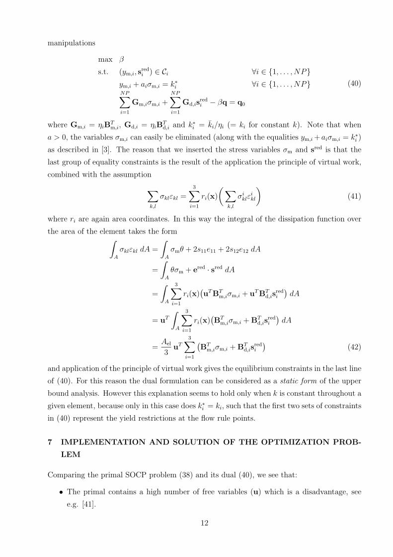
manipulations

max β

s.t. (ym,i, sredi ) ∈ Ci ∀i ∈ {1, . . . , NP}

ym,i + aiσm,i = k∗

i ∀i ∈ {1, . . . , NP}NP∑

i=1

Gm,iσm,i +NP∑

i=1

Gd,isredi − βq = q0

(40)

where Gm,i = ηiBTm,i, Gd,i = ηiB

Td,i and k∗

i = ki/ηi (= ki for constant k). Note that when

a > 0, the variables σm,i can easily be eliminated (along with the equalities ym,i +aiσm,i = k∗

i )

as described in [3]. The reason that we inserted the stress variables σm and sred is that the

last group of equality constraints is the result of the application the principle of virtual work,

combined with the assumption

∑

k,l

σklεkl =3

∑

i=1

ri(x)

(

∑

k,l

σiklε

ikl

)

(41)

where ri are again area coordinates. In this way the integral of the dissipation function over

the area of the element takes the form∫

A

σklεkl dA =

∫

A

σmθ + 2s11e11 + 2s12e12 dA

=

∫

A

θσm + ered · sred dA

=

∫

A

3∑

i=1

ri(x)(

uTBTm,iσm,i + uTBT

d,isredi

)

dA

= uT

∫

A

3∑

i=1

ri(x)(

BTm,iσm,i + BT

d,isredi

)

dA

=Ael

3uT

3∑

i=1

(

BTm,iσm,i + BT

d,isredi

)

(42)

and application of the principle of virtual work gives the equilibrium constraints in the last line

of (40). For this reason the dual formulation can be considered as a static form of the upper

bound analysis. However this explanation seems to hold only when k is constant throughout a

given element, because only in this case does k∗

i = ki, such that the first two sets of constraints

in (40) represent the yield restrictions at the flow rule points.

7 IMPLEMENTATION AND SOLUTION OF THE OPTIMIZATION PROB-

LEM

Comparing the primal SOCP problem (38) and its dual (40), we see that:

• The primal contains a high number of free variables (u) which is a disadvantage, see

e.g. [41].

12

• Linearly dependent equality constraints are less likely to appear in the dual; in fact

this can only happen if rigid body motion of the structure is permitted. In the primal

problem, dependencies may occur in the case of incompressible materials for some special

patterns of elements [10].

• The number of equality constraints in the primal (9 × NE + 1) is greater than that

in the dual (NU ≈ 4 × NE because the number of nodes is approximately twice the

number of elements, and each node has two degrees of freedom). The advantage might

be less pronounced when a = 0 because then the 3 × NE equalities ym,i + aσm,i = ki in

(40) cannot be eliminated.

• The number of cone constraints is the same in both problems.

Mainly because of the first two reasons, it seems that the dual formulation is preferable.

Computational experience [28], albeit for shakedown analysis using the von Mises criterion, has

shown that the dual can be solved in a significantly shorter CPU time. In general, however, this

will depend on the matrix manipulations employed by the optimization algorithm, and in our

case the effect might be different because the matrices Ai in (38) are diagonal. Nevertheless,

for reasons of stability (no free variables, no dependencies) it remains desirable to solve the

dual.

The following steps need to be followed in order to apply the proposed method. First,

calculation of the vectors q,q0 and the sub-matrices Gm,i,Gd,i for each flow rule point i.

Second, assembly of the constraint data in (40), and exportation to an appropriate format.

Third, solution of the optimization problem using a suitable algorithm/software. Since for

large discretizations both the primal (38) and dual (40) are highly sparse, i.e. there are very

few nonzero elements in each column, this immediately suggests that the use of an interior-

point algorithm would be advantageous. Also, the nature of the inequality constraints implies

that it would be more efficient to use an algorithm specialized for SOCP, rather than one

intended for general NLP problems, since we can conveniently avoid computational difficulties

arising from non-differentiability and Hessian singularity (see Section 1.3).

At present one of the leading algorithms for SOCP is that of Andersen et al. [36], which

has been implemented as part of MOSEK [42]. The algorithm has proved to be highly robust

and efficient in independent benchmark tests [43], which is why we have chosen it to solve

the numerical examples in the following section. It should however be noted that several

other SOCP solvers (both commercial and open-source) are currently available, and more will

undoubtedly appear in the future.

13

8 NUMERICAL EXAMPLES

The examples below are all plane strain problems involving the Mohr-Coulomb criterion.

For brevity we focus on the upper bound solutions and the efficiency with which they were

obtained, without entering into detailed interpretation or discussion of the respective dis-

placement fields. Each example is solved using both the simplex strain elements described in

Section 5, and the more usual configuration of constant strain elements combined with kine-

matically admissible discontinuities [4, 5, 6, 7], which we have also formulated as a standard

SOCP problem. The two element types will be referred to as “6-node elements” and “3-node

elements with discontinuities”.

The computations were performed on a Dell Pentium IV machine (2.66 GHz CPU, 2

GB RAM) in the Windows XP environment, using the conic interior-point optimizer of the

MOSEK package [42] mentioned above. For all analyses the default convergence tolerances of

the software were retained. The reported CPU times refer to the time actually spent on the

interior-point iterations, i.e. they exclude the time taken to read the data file (MPS format)

and execute the presolve routine. The presolve mainly involves reordering the rows of the

constraint matrix, and with 6-node elements this typically requires 15-25% of the CPU time

needed for the main optimization phase. The corresponding figure for 3-node elements with

discontinuities is rather higher, varying from 40% in some cases to 70% for the largest problems

analyzed in Section 8.3. This is possibly because the default node numbering generated by

the preprocessor is more suitable for continuous fields. The option to have MOSEK detect

and remove linearly dependent equality constraints during presolve was deactivated, since in

all cases the dual problem (i.e. the static form) was solved, such that no redundancies were

present (see Section 6).

8.1 Block with asymmetric holes

The plane strain test problem in Figure 3 has been studied by Zouain et al. [20], but only

for the von Mises criterion (i.e. not for cohesive-frictional material) and only using an ‘exact’

formulation of limit analysis based on mixed finite elements. For our upper bound analyses

we used GiD [44] to create three unstructured meshes of triangles with reduced element size

close to the holes. Two materials were considered: c = 1, φ = 0 and c = 1, φ = 30◦. The lower

bounds obtained in [3], namely pL = 1.809c for φ = 0 and pL = 1.056c for φ = 30◦, were used

to determine the average percentage error in bracketing the exact solution:

error =pU − pL

pU + pL× 100 (43)

In order to prevent rigid body translation and rotation of the structure, both degrees of free-

dom at the bottom left corner were restrained, together with the vertical degree of freedom at

14

the bottom right corner. This avoided the occurrence of linear dependencies in the constraint

matrix, without having any effect on the computed upper bounds.

Results obtained using 6-node elements and 3-node elements with discontinuities are given

in Tables 1 and 2 respectively. In both cases, despite the size of analyses (the Mesh 3 problems

contain nearly 180000 stress variables in the static form), very short CPU times and few

iterations are needed. This confirms the efficiency of the MOSEK optimizer and its ability to

handle large sparse SOCP problems. Comparing the performance of the elements, it is clear

that the 6-node version gives significantly better results, i.e. tighter upper bounds, though a

slightly greater CPU time is required for a given mesh and material. From a practical point of

view, it is more informative to compare the CPU times required to give results of comparable

accuracy. In this respect it is noteworthy that the coarsest mesh using 6-node elements gives

similar or better results than the finest mesh using 3-node elements with discontinuities, in

CPU times that are dramatically shorter (by a factor of approximately 40). Deformed shapes

of Mesh 1 for the purely cohesive material are shown in Figure 4. The analyses using 6-node

elements and 3-node elements with discontinuities both predict a similar arrangement of rigid

sliding blocks, separated by zones of intense shearing that originate from the holes.

For the purely cohesive material it is also interesting to make a comparison with the results

of Zouain et al. [20], who used mixed 6-node triangular elements with continuous quadratic

displacements and discontinuous stresses. Within each of their elements the deviatoric stresses

varied linearly, but the mean stress was constant. The limit loads obtained (using the von

Mises criterion) were 1.052σy for an initial mesh of 716 elements, and 1.035σy for an improved

mesh after refinement. In terms of the Tresca criterion, these results correspond to 1.822c and

1.793c respectively (cf. 2c for a block with no holes). We notice that our upper bound results

in Tables 1 and 2 are higher, as might be expected, however it is surprising that Zouain et

al.’s improved result of 1.793c is lower than the lower bound of 1.809c we obtained in [3]. The

areas of higher dissipation in our analyses (see Figure 5) correspond quite closely to the finely

discretized regions of the improved mesh in Zouain et al. [20], so their refinement seems to

be targeted correctly. A possible explanation for the disagreement in the computed limit load

is that their error estimator is related to the displacement field, however the simultaneous

discretization of the stress field may lead to lower results (compared with discretizing only the

displacement field) because the mean stress is constrained to be constant over each element.

8.2 Strip footing bearing capacity

On weightless Mohr-Coulomb soil (c ≥ 0, φ ≥ 0, γ = 0) in the absence of surcharge, the

bearing capacity of a rigid, symmetrically loaded strip footing of width B is given by

Q

B= cNc (44)

15

where Q is the limit load (force per unit length) and Nc is a dimensionless bearing capacity

factor that depends on φ. Exact values of Nc can be determined using the well known equation

of Prandtl [45]:

Nc =

[

eπ tan φ tan2(π

4+

φ

2

)

− 1

]

cot φ (45)

Note that if φ = 0 then Nc = 2 + π. Another fundamental case is that of ponderable

cohesionless soil (c = 0, φ > 0, γ > 0) with no surcharge; the bearing capacity is then

traditionally expressed asQ

B=

1

2γBNγ (46)

where Nγ is another dimensionless factor that depends on φ. At present there is no analytical

solution for Nγ, but it can be evaluated using a variety of numerical methods. To assist with

benchmarking exercises such as this, the second author has recently published a selection

of high-precision Nγ values for both smooth and rough footings [46]. These numbers (for

φ = 5◦, 10◦, . . . , 45◦) were obtained using the method of stress characteristics, though they have

now been checked using an alternative technique (Runge-Kutta integration of the governing

ordinary differential equations), and also formally confirmed as exact plasticity solutions [47].

The footing problem is one of the most widely used benchmarks in limit analysis, though

in most cases it has only been examined for the case of purely cohesive soil (φ = 0). Another

observation is that when the soil is weightless, the bearing capacity of a rigid footing is

the same as that under a uniform pressure load, and many researchers choose to solve the

latter problem when evaluating Nc (see e.g. [13, 27]). However the rigid boundary condition

represents a more difficult problem since the displacement field is more constrained, and this

is the case that we examine. Finally, it is well known that when using finite elements the

difficulty of the problem increases with φ, and with the ratio γB/c (i.e. the Nγ problem is

considerably harder to solve than the Nc problem, see e.g. [48]).

Several upper bound analyses of rigid footings on purely cohesive and cohesive-frictional

soil have been made by Sloan and co-workers [5, 7, 49], in all cases using 3-node elements with

discontinuities. The calculations of Nc by Sloan and Kleeman [5] were extremely satisfactory

for φ = 0 (only 1.4% error). The effectiveness was reduced for φ = 30◦ (5.4% error), but this

result could also be considered satisfactory as the number of elements employed was quite

small. It is important to note, however, that the meshes were very carefully designed, with

the orientation of the discontinuities seemingly based on the slip-lines in Prandtl’s analytical

solution. In the work of Lyamin and Sloan [7] the result for Nc when φ = 35◦ was again very

good (2.5% error with 917 elements), but the mesh again appeared to have been generated

with the help of the slip-line method. Similar careful attention to mesh design was apparent

in the study by Hjiaj et al. [49] concerning the calculation of Nγ; in fact numerous different

meshes were employed, depending on the value of φ and the footing roughness. A question

arising is this: how effective might analyses with unstructured meshes be?

16

For the present work, GiD [44] was used to generate three unstructured meshes with

reduced element size close to the footing. The displacement boundary conditions and the

dimensions of the soil domain are shown in Figure 6, and the coarsest of the three meshes is

shown in Figure 7. In the initial set of analyses, the footing was assumed to be smooth and

upper bounds were determined for the factors Nc (φ = 0, 35◦) and Nγ (φ = 35◦). Tables 3

(6-node elements) and 4 (3-node elements with discontinuities) show how the results compare

with the respective exact solutions: Nc = 5.142, Nc = 46.12 and Nγ = 17.58. Displacement

vectors for the various cases are shown in Figure 8. The following comments can be made:

• As expected, the error in Nc is greater for cohesive-frictional soil than for purely cohesive

soil, and the error in Nγ (which pertains to purely frictional soil) is greater still.

• In the case of purely cohesive soil, the results from the two element types are very

similar. The same conclusion was drawn by Yu et al. [8], who compared 6-node and

3-node elements for special mesh patterns and selected discontinuities.

• In both analyses with φ = 35◦, the errors obtained using 3-node elements with discon-

tinuities are large (> 10% even for a huge number of elements). By comparison, the

6-node elements are very satisfactory, giving errors of just 0.5% for Nc and 1.2% for Nγ

using Mesh 3.

• For the same mesh and soil parameters, analyses with the two different element types

require quite similar CPU times. As in the previous example, the optimization timings

are slightly better for the 3-node elements with discontinuities, though this is offset by

a longer time spent in the presolve phase (see the introduction to Section 8).

• In all cases the problems are solved in very few iterations, and with great speed.

It is clear that the calculation of Nγ is the most challenging benchmark, and for this reason

a second set of analyses was performed. A single unstructured mesh of 31481 elements (not

pictured) was generated using GiD and used to compute upper bounds on Nγ for both smooth

and rough footings, for friction angles ranging from 5◦ to 45◦. The results are given in Tables 5

(6-node elements) and 6 (3-node elements with discontinuities). We notice now that the rough

footing poses an even harder test than the smooth footing, especially in the case of the largest

friction angle. Nevertheless, our upper bounds are all consistent with (i.e. above) the exact

values, and together with the even more satisfactory lower bounds obtained in [3], provide

excellent bracketing. A comparison of Tables 5 and 6 indicates that the accuracy of the 3-node

element with discontinuities is acceptable only for low values of φ, whereas the 6-node element

gives good performance (generally 1-2% error) over the full range. The problems involving

3-node elements with discontinuities are solved in slightly shorter CPU times, though again it

17

should be noted that a longer presolve is necessary (typically 40 s, as against 20 s for 6-node

elements) such that there is no significant difference in the overall timings.

It is worth comparing the present results with those of Hjiaj et al. [49], which were obtained

using case-specific structured meshes of up to 20815 3-node elements with discontinuities. Over

the same range of φ, the errors in their upper bound values of Nγ range from 4.8-8.2% for

smooth footings and 2.8-5.5% for rough footings. The comparable figures from our analyses,

all of which were performed using the same unstructured mesh of 31481 6-node elements, are

0.4-1.5% and 1.2-3.9% as shown in Table 5. We emphasize again that while the meshes of Hjiaj

et al. were individually tailored depending on the friction angle and the footing roughness,

our results were obtained using an identical mesh for all combinations of parameters, and this

is more in keeping with the basic philosophy of the finite element method. A final observation

on the results of Hjiaj et al. [49] is that several of their lower bound solutions (smooth footing

φ = 5◦, 10◦, 15◦ and rough footing φ = 5◦) are greater than the exact values of Nγ, and

in certain cases (smooth footing φ = 5◦, 10◦) their lower bounds are even greater than our

upper bounds. It has subsequently emerged that the analyses of Hjiaj et al. were not in fact

performed with c = 0, but with a nominal cohesion that had to be introduced for numerical

reasons (Lyamin, personal communication, 2005).

8.3 Slope stability

In this example we consider the stability of a homogeneous slope of cohesive-frictional soil

having inclination 70◦ and height H. The quantity of interest in the limit load calculation is

the critical value of the stability factor Ns = γH/c. To obtain an upper bound solution, it is

convenient to consider c = 1, H = 1 and (recalling that we solve the static form) maximize

the unit weight γ.

Analyses were performed for two friction angles (20◦ and 35◦) and several different levels

of mesh refinement. Both unstructured and ‘semi-uniform’ meshes were employed; Figure

9 shows meshes of each type containing approximately 4000 elements. As in the previous

examples, the performance of both 6-node elements and 3-node elements with discontinuities

was examined for each mesh. Since there is no exact solution for the homogeneous slope

problem, it is convenient to assess the accuracy of the finite element upper bounds with

reference to those tabulated by Chen [50]:

NUs = 8.30 for φ = 20◦

NUs = 13.86 for φ = 35◦

(47)

Despite the simplicity of his log-spiral mechanism, Chen’s upper bounds must be very close

to optimal, since lower bounds obtained using the method described in [3] are only about 1%

18

lower:NL

s = 8.210 for φ = 20◦

NLs = 13.75 for φ = 35◦

(48)

Statistics and results for the present upper bound analyses are shown in Tables 7,8 (unstruc-

tured meshes) and Tables 9,10 (semi-uniform meshes). Some selected graphical outputs are

shown in Figures 10 and 11. From the data we see that:

• The problem is much more difficult for φ = 35◦ than for φ = 20◦ since in all cases

we get much greater errors. The growth in the error with friction angle is particularly

pronounced when using 3-node elements with discontinuities.

• For unstructured meshes, the performance of the 3-node element with discontinuities is

poor, especially when φ = 35◦. The performance of the 6-node element is satisfactory

for φ = 20◦, and although it deteriorates somewhat for φ = 35◦, it still outperforms the

lower-order element with ease. For example, 4132 6-node elements give a better result

than 28864 3-node elements with discontinuities, in an order of magnitude less CPU

time.

• For semi-uniform meshes, there is a substantial improvement in the results, i.e. we get

much lower upper bounds. The 6-node element again gives better performance, though

the results obtained using 3-node elements with discontinuities are now respectable,

especially for φ = 20◦. This improvement is of course expected, since the NE-SW

division of each quadrant into two triangles assists the development of discontinuities in

the collapse mechanism (see Figure 10(b). However it is interesting that this topology

also helps the 6-node elements, even though the displacement field is continuous (Figure

10(a)).

• The results from unstructured meshes of 6-node elements (Table 7) and semi-uniform

meshes of 3-node elements with discontinuities (Table 10) are quite similar for φ = 20◦,

but the 6-node element gives much better performance for φ = 35◦.

• In all cases (with one exception where many iterations were spent close to the final

solution) the interior-point algorithm required fewer than 30 iterations.

Upper bound solutions for the homogeneous slope stability problem have also been pre-

sented by Krabbenhoft et al. [34], for inclinations from 50◦ to 90◦. They used 4160 3-node

elements with discontinuities in a wholly structured mesh where the quadrilaterals in the slope

were subdivided into four triangles (rather than two) by intersecting the diagonals; they also

employed gradual transitions in the element size in both the horizontal and vertical direc-

tions. For φ = 20◦ (the easier case above) they obtained NUs = 8.44. The result from our

unstructured mesh of 4132 6-node elements is higher (8.617), while our semi-uniform mesh of

19

4306 6-node elements does slightly better (8.400). The corresponding results from our very

fine meshes, see Tables 7 and 9, are 8.338 and 8.283 respectively. Unfortunately Krabbenhoft

et al. [34] did not report any results for more challenging friction angles. However the most

important point of comparison between the two studies is the ability of MOSEK – using its

default settings – to solve much larger problems (more than ten times as many elements) in

CPU times that remain very modest (a few minutes at most). By coupling a powerful SOCP

optimizer with the accuracy of the simplex strain element, we have shown that very tight

upper bounds can be obtained for this difficult problem, even using unstructured meshes.

9 CONCLUSIONS

This paper has presented a new method for upper bound limit analysis of cohesive-frictional

materials, using displacement finite elements and second-order cone programming (SOCP). It

has been shown that for any convex yield function, rigorous upper bounds can be obtained

using a continuous quadratic displacement field, provided that the strains within each element

vary as a simplex (6-node triangles and 10-node tetrahedra must have straight sides and plane

faces respectively). Several plane strain benchmark problems have been used to demonstrate

that this approach gives better results than the usual piecewise linear displacement field,

particularly in the case of unstructured meshes and/or materials with high friction angles. For

a given problem (same mesh, same material) the computational cost is broadly similar. Of

course our formulation does not ‘reject’ the use of discontinuous displacement fields, however

it is clear that if there is no a priori knowledge of the collapse mechanism, then we are unable

to take full advantage of discontinuities by ensuring that they are suitably aligned. Possibly

the most efficient solution would be to combine both approaches by implementing some form

of adaptive slip-line detection.

From a computational viewpoint, SOCP provides the most natural framework for limit

analysis of discretized structures where the yield function can be expressed in a conic quadratic

form (e.g. Drucker-Prager in plane stress, plane strain or 3D; Mohr-Coulomb in plane strain;

Nielsen’s criterion for plates). The efficient computation of strict lower bound solutions using

SOCP has already been treated in detail in [3]. Here a corresponding formulation of upper

bound analysis has again allowed us to apply a primal-dual interior-point algorithm specialized

for SOCP, and obtain similar benefits. Without any tuning of its default settings, MOSEK

[42] has been used to solve some very large problems with remarkable speed, though it should

be emphasized that these are by no means the largest upper bound analyses that the software

can handle. They are, however, much larger than those recently performed by Sloan and

co-workers [7, 34]. For comparable meshes our CPU times would also appear to be faster, but

this is unsurprising given that Sloan and co-workers employ a general NLP algorithm for use

with arbitrary smooth yield functions, whereas SOCP is ideally suited (but also restricted)

20

to conic quadratic yield functions. As mentioned above, several of the classical yield criteria

of geomechanics fall into this category, and in these cases the use of SOCP allows rapid and

tight bracketing of the exact limit load. An additional benefit is that there is no need to use

any ad hoc smoothing strategy for cohesive-frictional materials, where the yield function has

a non-differentiable apex point.

Acknowledgment

The first author would like to thank professor C. Bisbos (Aristotle University of Thessaloniki)for recommending to him the work of Salencon concerning the dissipation functions.

REFERENCES

[1] Gvozdev AA. The determination of the value of the collapse load for statically indeterminate systems

undergoing plastic deformation (in Russian). In Conference on Plastic Deformations 1936, Galerkin BG

(ed). Akademia Nauk SSSR: Moscow and Leningrad, 1938; 19–38.

[2] Drucker DC, Prager W, Greenberg HJ. Extended limit design theorems for continuous media. Quarterly

of Applied Mathematics 1952; 9:381–389.

[3] Makrodimopoulos A, Martin CM. Lower bound limit analysis of cohesive-frictional materials using second-

order cone programming. Technical Report No. OUEL 2278/05, University of Oxford, 2005.

[4] Bottero A, Negre R, Pastor J, Turgeman S. Finite element method and limit analysis theory for soil

mechanics problems. Computer Methods in Applied Mechanics and Engineering 1980; 22:131–149.

[5] Sloan SW, Kleeman PW. Upper bound limit analysis using discontinuous velocity fields. Computer Methods

in Applied Mechanics and Engineering 1995; 127:293–314.

[6] Pastor J, Thai TH, Francescato P. New bounds for the height limit of a vertical slope. International

Journal for Numerical and Analytical Methods in Geomechanics 2000; 24:165–182.

[7] Lyamin AV, Sloan SW. Upper bound analysis using linear finite elements and non-linear programming.

International Journal for Numerical and Analytical Methods in Geomechanics 2002; 26:181–216.

[8] Yu HS, Sloan SW, Kleeman PW. A quadratic element for upper bound limit analysis. Engineering Com-

putations 1994; 11:195–212.

[9] Pastor J, Loute E, Thai TH. Limit analysis and new methods of optimization. Proceedings of the 5th

European Conference on Numerical Methods in Engineering, Paris 2002; 211–219.

[10] Nagtegaal JC, Parks DM, Rice JR. On numerically accurate finite element solutions in the fully plastic

range. Computer Methods in Applied Mechanics and Engineeering 1974; 4:153–177.

[11] Sloan SW, Randolph MF. Numerical prediction of collapse loads using finite element methods. Interna-

tional Journal for Numerical and Analytical Methods in Geomechanics 1982; 6:47–76.

[12] Yu HS, Houlsby GT, Burd HJ. A novel isoparametric finite element displacement formulation for ax-

isymmetric analysis of nearly incompressible materials. International Journal for Numerical Methods in

Engineering 1993; 36:2453–2472.

21

[13] Tin-Loi F, Ngo NS. Performance of the p-version finite element method for limit analysis. International

Journal of Mechanical Sciences 2003; 45:1149–1166.

[14] Maier G. Shakedown theory in perfect elastoplasticity with associated and non-associated flow laws: a

finite element linear programming approach. Meccanica 1969; 4:250–260.

[15] Sloan SW. Upper bound limit analysis using finite elements and linear programming. International Jour-

nal for Numerical and Analytical Methods in Geomechanics 1989; 13:263–282

[16] Andersen KD, Christiansen E. Limit analysis with the dual affine scaling algorithm. Journal of Compu-

tational and Applied Mathematics 1995; 59:233–243.

[17] Belytschko T, Hodge PG. Plane stress limit analysis by finite elements. Journal of the Engineering

Mechanics Division, ASCE 1970; 96:931–944.

[18] Gao Y. Panpenalty finite element programming for plastic limit analysis. Computers & Structures 1988;

28:749–755.

[19] Zouain N, Herskovits J, Borges LA, Feijoo RA. An iterative algorithm for limit analysis with nonlinear

yield functions. International Journal of Solids and Structures 1993; 30:1397–1417.

[20] Zouain N, Borges LA, Silveira JL. An algorithm for shakedown analysis with nonlinear yield functions.

Computer Methods in Applied Mechanics and Engineering 2002; 191:2463–2481.

[21] Christiansen E, Andersen KD. Computation of collapse states with von Mises type yield condition.

International Journal for Numerical Methods in Engineering 1999; 46:1185–1202.

[22] Andersen KD, Christiansen E, Conn A, Overton ML. An efficient primal-dual interior-point method for

minimizing a sum of Euclidean norms. SIAM Journal on Scientific Computing 2000; 22:243–262.

[23] Ponter ARS, Fuschi P, Engelhardt M. Limit analysis for a general class of yield conditions. European

Journal of Mechanics A/Solids 2000; 19:401–421.

[24] Lyamin AV, Sloan SW. Lower bound limit analysis using non-linear programming. International Journal

for Numerical Methods in Engineering 2002; 55:573–611.

[25] Krabbenhoft K, Damkilde L. A general non-linear optimization algorithm for lower bound limit analysis.

International Journal for Numerical Methods in Engineering 2003; 56:165–184.

[26] Yang H, Shen Z, Wang J. 3D lower bound bearing capacity of smooth rectangular surface footings.

Mechanics Research Communications 2003; 30:481–492.

[27] Li HX, Yu HS. Kinematic limit analysis of frictional materials using nonlinear programming. International

Journal of Solids and Structures 2005; 42:4058–4076.

[28] Makrodimopoulos A. Computational approaches to shakedown phenomena of metal structures under

plane and axisymmetric stress states (in Greek). PhD Thesis, Aristotle University of Thessaloniki, Greece,

2001.

[29] Makrodimopoulos A, Bisbos C. Shakedown analysis of plane stress problems via SOCP. In Numerical

Methods for Limit and Shakedown Analysis, Staat M, Heitzer M (eds). John von Neumann Institute for

Computing (NIC): Julich, 2003; 185–216.

22

[30] Ciria H, Peraire J. Computation of upper and lower bounds in limit analysis using second-order cone pro-

gramming and mesh adaptivity. 9th ASCE Specialty Conference on Probabilistic Mechanics and Structural

Reliability, Albuquerque 2004; 13 pp.

[31] Bisbos C, Makrodimopoulos A, Pardalos PM. Second-order cone programming approaches to static shake-

down analysis in steel plasticity. Optimization Methods and Software 2005; 20:25–52.

[32] Makrodimopoulos A. Computational formulation of shakedown analysis as a conic quadratic optimization

problem. Mechanics Research Communications 2005; in press.

[33] Trillat M, Pastor J, Francescato P. Yield criterion for porous media with spherical voids. Mechanics

Research Communications 2005; in press.

[34] Krabbenhoft K, Lyamin AV, Hjiaj M, Sloan SW. A new discontinuous upper bound limit analysis for-

mulation. International Journal for Numerical Methods in Engineering 2005; 63:1069–1088.

[35] Salencon J. Applications of the Theory of Plasticity in Soil Mechanics. Wiley: Chichester, 1977.

[36] Andersen ED, Roos C, Terlaky T. On implementing a primal-dual interior-point method for conic

quadratic optimization. Mathematical Programming Series B 2003; 95:249–277.

[37] Tsuchiya T. A polynomial primal-dual path-following algorithm for second-order cone programming.

Research Memorandum No. 649, The Institute of Statistical Mathematics, Tokyo, 1997.

[38] Andersen ED, Roos C, Terlaky T. Notes on duality in second order and p-order cone optimization.

Optimization 2002; 51:627–643.

[39] Drucker DC, Prager W. Soil mechanics and plastic analysis or limit design. Quarterly of Applied Mathe-

matics 1952; 10:157–165.

[40] Salencon J. Yield design: a survey of the theory. In Evaluation of global bearing capacities of structures,

Sacchi Landriani G, Salencon J (eds). Springer-Verlag: Wien, 1993; 1–44.

[41] Meszaros C. On free variables in interior point methods. Optimization Methods and Software 1998; 9:121–

139.

[42] MOSEK ApS. The MOSEK optimization tools version 3.2 (Revision 8). User’s manual and reference.

Available from http://www.mosek.com [January 2005].

[43] Mittelmann HD. An independent benchmarking of SDP and SOCP solvers. Mathematical Programming

2003; 95:407–430.

[44] International Centre For Numerical Methods In Engineering (CIMNE). GiD version 7.0. Reference man-

ual. Available from http://gid.cimne.upc.es [January 2005].

[45] Prandtl L. Uber die Eindringungsfestigkeit (Harte) plastischer Baustoffe und die Festigkeit von Schneiden.

Zeitschrift fur angewandte Mathematik und Mechanik 1921; 1:15–20.

[46] Martin CM. Discussion of “Calculations of bearing capacity factor Nγ using numerical limit analyses” by

Ukritchon et al. Journal of Geotechnical and Geoenvironmental Engineering, ASCE 2004; 130:1106–1107.

[47] Martin CM. Exact bearing capacity calculations using the method of characteristics. Proceedings of the

11th International Conference of IACMAG, Turin 2005; 4:441–450.

23

[48] Ukritchon B, Whittle AJ, Klangvijit C. Calculations of bearing capacity factor Nγ using numerical limit

analyses. Journal of Geotechnical and Geoenvironmental Engineering, ASCE 2003; 129:468–474.

[49] Hjiaj M, Lyamin AV, Sloan SW. Numerical limit analysis solutions for the bearing capacity factor Nγ .

International Journal of Solids and Structures 2005; 42:1681–1704.

[50] Chen WF. Limit Analysis and Soil Plasticity. Elsevier: Amsterdam, 1975.

24

Table 1: Results for block with asymmetric holes (6-node elements).φ = 0 φ = 30◦

Mesh NE DOF NVS p/c CPU (s) p/c CPU (s)(error %) (iter) (error %) (iter)

1 814 3455 7326 1.867 1.0 1.077 0.8(1.59) (16) (0.96) (16)

2 4446 18583 40014 1.845 7.3 1.070 5.3(1.00) (20) (0.66) (16)

3 19714 79955 177426 1.825 51.2 1.063 53.1(0.44) (17) (0.30) (24)

NE = no. of elements, DOF = degrees of freedom, NVS = no. of stress variables in dual

Table 2: Results for block with asymmetric holes (3-node elements with discontinuities).φ = 0 φ = 30◦

Mesh NE DOF NVS p/c CPU (s) p/c CPU (s)(error %) (iter) (error %) (iter)

1 814 4881 7122 1.923 0.7 1.106 0.6(3.06) (20) (2.29) (18)

2 4446 26673 39210 1.896 5.0 1.104 4.7(2.35) (21) (2.19) (21)

3 19714 118281 176322 1.864 39.0 1.081 31.1(1.49) (21) (1.16) (22)

NE = no. of elements, DOF = degrees of freedom, NVS = no. of stress variables in dual

25

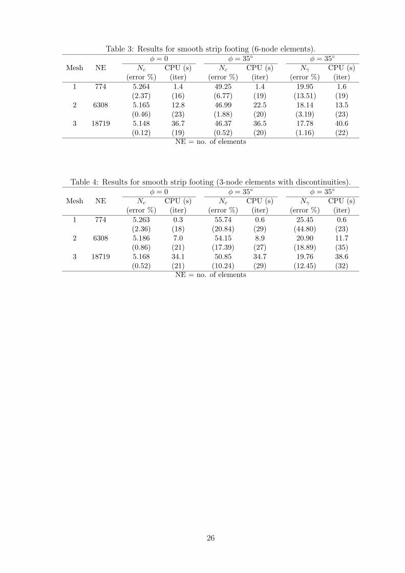
Table 3: Results for smooth strip footing (6-node elements).φ = 0 φ = 35◦ φ = 35◦

Mesh NE Nc CPU (s) Nc CPU (s) Nγ CPU (s)(error %) (iter) (error %) (iter) (error %) (iter)

1 774 5.264 1.4 49.25 1.4 19.95 1.6(2.37) (16) (6.77) (19) (13.51) (19)

2 6308 5.165 12.8 46.99 22.5 18.14 13.5(0.46) (23) (1.88) (20) (3.19) (23)

3 18719 5.148 36.7 46.37 36.5 17.78 40.6(0.12) (19) (0.52) (20) (1.16) (22)

NE = no. of elements

Table 4: Results for smooth strip footing (3-node elements with discontinuities).φ = 0 φ = 35◦ φ = 35◦

Mesh NE Nc CPU (s) Nc CPU (s) Nγ CPU (s)(error %) (iter) (error %) (iter) (error %) (iter)

1 774 5.263 0.3 55.74 0.6 25.45 0.6(2.36) (18) (20.84) (29) (44.80) (23)

2 6308 5.186 7.0 54.15 8.9 20.90 11.7(0.86) (21) (17.39) (27) (18.89) (35)

3 18719 5.168 34.1 50.85 34.7 19.76 38.6(0.52) (21) (10.24) (29) (12.45) (32)

NE = no. of elements

26

Table 5: Results for bearing capacity factor Nγ (6-node elements).Smooth Rough Exact values

φ (◦) Nγ CPU (s) Nγ CPU (s) smooth rough(error %) (iter) (error %) (iter)

5 0.08485 80 0.1159 80 0.08446 0.1134(0.46) (23) (2.21) (24)

10 0.2820 77 0.4399 82 0.2809 0.4332(0.41) (22) (1.55) (24)

15 0.7027 82 1.196 87 0.6991 1.181(0.52) (24) (1.26) (26)

20 1.586 79 2.872 81 1.579 2.839(0.44) (23) (1.16) (24)

25 3.479 79 6.568 78 3.461 6.491(0.50) (23) (1.18) (23)

30 7.700 78 14.96 77 7.653 14.75(0.61) (23) (1.37) (23)

35 17.71 79 35.10 99 17.58 34.48(0.76) (23) (1.81) (28)

40 43.62 81 87.81 94 43.19 85.57(1.00) (24) (2.62) (26)

45 119.4 89 243.5 104 117.6 234.2(1.52) (26) (3.95) (30)

27

Table 6: Results for bearing capacity factor Nγ (3-node elements with discontinuities).Smooth Rough Exact values

φ (◦) Nγ CPU (s) Nγ CPU (s) smooth rough(error %) (iter) (error %) (iter)

5 0.08591 66 0.1175 52 0.08446 0.1134(1.71) (29) (3.62) (25)

10 0.2853 66 0.4470 55 0.2809 0.4332(1.56) (29) (3.20) (26)

15 0.7162 58 1.223 56 0.6991 1.181(2.45) (26) (3.49) (27)

20 1.617 60 2.955 56 1.579 2.839(2.40) (28) (4.09) (27)

25 3.598 60 6.864 63 3.461 6.491(3.96) (28) (5.74) (30)

30 8.160 62 15.98 69 7.653 14.75(6.63) (29) (8.34) (33)

35 19.204 68 38.78 75 17.58 34.48(9.25) (31) (12.48) (35)

40 48.22 75 104.1 86 43.19 85.57(11.66) (35) (21.70) (41)

45 138.3 84 309.0 96 117.6 234.2(17.62) (38) (31.92) (44)

28

Table 7: Results for 70◦ slope (unstructured meshes, 6-node elements).φ = 20◦ φ = 35◦

Mesh NE Ns CPU (s) Ns CPU (s)(diff %) (iter) (diff %) (iter)

1 1629 8.854 2.4 15.72 2.8(6.67) (20) (13.39) (18)

2 4132 8.617 7.9 14.97 9.3(3.82) (21) (7.98) (21)

3 8921 8.469 25.1 14.45 24.6(2.04) (23) (4.23) (23)

4 28864 8.338 194.5 14.19 109.5(0.46) (36) (2.41) (21)

NE = no. of elements; differences w.r.t. upper bounds of Chen [50]

Table 8: Results for 70◦ slope (unstructured meshes, 3-node elements with discontinuities).φ = 20◦ φ = 35◦

Mesh NE Ns CPU (s) Ns CPU (s)(diff %) (iter) (diff %) (iter)

1 1629 9.372 1.7 18.13 2.1(12.92) (21) (30.77) (25)

2 4132 8.896 5.4 16.95 4.5(7.18) (22) (22.27) (18)

3 8921 8.647 18.5 15.68 19.3(4.18) (25) (13.11) (27)

4 28864 8.471 65.1 15.46 85.2(2.06) (23) (11.57) (29)

NE = no. of elements; differences w.r.t. upper bounds of Chen [50]

29

Table 9: Results for 70◦ slope (semi-uniform meshes, 6-node elements).φ = 20◦ φ = 35◦

Mesh NE Ns CPU (s) Ns CPU (s)(diff %) (iter) (diff %) (iter)

1 4306 8.400 7.4 14.16 10.0(1.20) (18) (2.13) (26)

2 28813 8.304 112.0 13.93 117.0(0.05) (23) (0.47) (21)

3 54427 8.283 302.2 13.88 323.3(-0.20) (23) (0.13) (24)

NE = no. of elements; differences w.r.t. upper bounds of Chen [50]

Table 10: Results for 70◦ slope (semi-uniform meshes, 3-node elements with discontinuities).φ = 20◦ φ = 35◦

Mesh NE Ns CPU (s) Ns CPU (s)(diff %) (iter) (diff %) (iter)

1 4306 8.528 6.0 15.04 6.3(2.75) (20) (8.50) (21)

2 28813 8.405 72.6 14.48 62.0(1.27) (25) (4.44) (21)

3 54427 8.366 138.6 14.31 149.9(0.80) (21) (3.28) (23)

NE = no. of elements; differences w.r.t. upper bounds of Chen [50]

30

Figure 1: The set of plastically admissible strains for the Drucker-Prager criterion.

31

Figure 2: 6-node displacement element for upper bound analysis.

32

Figure 3: Block with asymmetric holes (after Zouain et al. [20]).

33

(a)

(b)

Figure 4: Deformed shape for block with asymmetric holes (c = 1, φ = 0, Mesh 1). (a) 6-nodeelements (b) 3-node elements with discontinuities.

34

(a) Mesh 1 (814 elements)

(b) Mesh 2 (4446 elements)

(c) Mesh 3 (19714 elements)

Figure 5: Dissipation function for block with asymmetric holes (c = 1, φ = 0, 6-node elements).

35

Figure 6: Boundary conditions and mesh dimensions for strip footing.

36

Figure 7: Mesh 1 (774 elements) for smooth strip footing.

37

c=1, f=0°

c=1, f=35°

c=0, f=35°

(a) = 1, = 0, = 0c f g

(b) = 1, = 35 , = 0c f ° g

(c) = 0, = 35 , = 1c f g°

c=1, f=0

c=1, f=35°

c=0, f=35°

(d) = 1, = 0, = 0c f g

(e) = 1, = 35 , = 0c f ° g

(f) = 0, = 35 , = 1c f g°

Figure 8: Displacement field close to smooth strip footing (Mesh 1). (a)-(c) 6-node elements(d)-(f) 3-node elements with discontinuities.

38

(a)

(b)

Figure 9: 70◦ slope: (a) unstructured Mesh 2 (4132 elements) (b) semi-uniform Mesh 1 (4306elements).

39

φ=35° φ=35°

(a) (b)

Figure 10: Deformed shape for 70◦ slope (c = 1, φ = 35◦, semi-uniform Mesh 1). (a) 6-nodeelements (b) 3-node elements with discontinuities.

40

(a) = 1, = 20c f ° (b) = 1, = 35c f °

Figure 11: Dissipation function for 70◦ slope (unstructured Mesh 4, 6-node elements).

41