Unsupervised nonparametric detection of unknown objects …

Unsupervised nonparametricdetection of unknown objects in noisy

images based on percolation theory

Mikhail Langovoy∗

Machine Learning and Optimization LaboratoryEPFL, Station 14

Lausanne, CH-1015 Switzerlande-mail: [email protected]

and

Olaf Wittich

Lehrstuhl A fur MathematikRWTH Aachen, 52056 Aachen

e-mail: [email protected]

and

Laurie Davies

Department of Statistics,University of California at Davis, Davis CA,

95616-8572, USAe-mail: [email protected]

Abstract: We develop an unsupervised, nonparametric, and scalablestatistical learning method for detection of unknown objects in noisyimages. The method uses results from percolation theory and randomgraph theory. We present an algorithm that allows to detect objectsof unknown shapes and sizes in the presence of nonparametric noise ofunknown level. The noise density is assumed to be unknown and canbe very irregular. The algorithm has linear complexity and exponen-tial accuracy and is appropriate for real-time systems. We prove strongconsistency and scalability of our method in this setup with minimalassumptions.

Keywords and phrases: Nonparametric learning, unsupervised learn-ing, object detection, image analysis, noisy image, percolation, extremenoise, nonparametric hypothesis testing.

∗Corresponding author.

1imsart-generic ver. 2007/04/13 file: Detection_Percolation_Version_6.tex date: August 30, 2021

arX

iv:1

102.

5019

v2 [

mat

h.ST

] 1

2 Ju

l 201

8

mailto:[email protected]



M. Langovoy et al./Unsupervised detection and percolation 2

1. Introduction

Detection of objects in noisy images is the most basic problem of imageanalysis. Indeed, when one looks at a noisy image, the first question to askis whether there is any object hidden behind the noise, at all. This is alsoa primary question of interest in such diverse fields as, for example, cancerdetection (Ricci-Vitiani et al., 2007), automated urban analysis (Negri et al.,2006), detection of cracks in buried pipes (Sinha and Fieguth, 2006), andother possible applications in astronomy, electron microscopy and neurology.Moreover, if there is just a random noise in the picture, it doesn’t make senseto run computationally intensive procedures for image reconstruction for thisparticular picture. This is especially relevant in modern day applications toInternet data and in automated image processing systems, where one has tomine billions of images under time constraints. Surprisingly, the vast majorityof image analysis methods, both in statistics and in engineering, avoid thepure detection problem and start immediately with the more challenging andcomputationally intensive task of image reconstruction.

1.1. Related work

As pixels in digital images can be viewed as network nodes with attributes,many applications from image processing, such as road tracking (Gemanand Jedynak, 1996) or medical tumor detection (McInerney and Terzopou-los, 1996), can be treated within the framework of community detection innetworks. More specifically, these setups correspond to detection of commu-nities hidden in large networks with noisy node attributes, where one decideson the existence of communities using both the network topology as well asthe network’s content represented by node attributes (see, e.g., (Ruan et al.,2013) or (Yang et al., 2013) for related types of setups).

We are only concerned with the existence of an object in the image, andnot with estimating the object. We are also heavily using the fact that imagesare processed on computers only in a discretized form. For this problem andthe setup, recently a new line of research emerged where discrete probabilitymethods of statistical physics were applied to unsupervised community de-tection in discrete structures such as pixelized images or lattices (Langovoyand Wittich, 2009), (Langovoy and Wittich, 2013a), (Langovoy and Wittich,2013b), (Arias-Castro and Grimmett, 2013). The idea of applying percolationtheory to study of hidden communities in networks, combined with variationsof k-NN scans, proved useful in application areas like anomaly detection andautomated detection of unknown objects in extremely noisy images (Lan-govoy et al., 2011b), (Langovoy et al., 2011a).

imsart-generic ver. 2007/04/13 file: Detection_Percolation_Version_6.tex date: August 30, 2021


However, in (Arias-Castro and Grimmett, 2013) only the case of paramet-ric noise from a one-parameter exponential family was considered, while thepresent paper deals with the general case of nonparametric noise. Our bulkcondition on the object interior is also more general than conditions on clus-ter sizes in (Arias-Castro and Grimmett, 2013). The algorithm in the presentpaper has linear computational complexity, irrespectively of a shape of anobject. Papers (Langovoy and Wittich, 2009) and (Langovoy and Wittich,2013a) treated different kind of underlying lattices and had to resort to thecase of nonparametric noise of bounded level, while (Langovoy and Wittich,2013b) had to limit the class of possible noise distributions via additionalsmoothness assumptions. In this paper, we establish a strong form of consis-tent detection for a much wider class of noise distributions, and completelyremove smoothness assumptions on the noise.

1.2. Main contributions

From the statistical point of view, we treat the object detection problemas a nonparametric hypothesis testing problem within the class of statisticalinverse problems on networks. We assume that the noise density is completelyunknown, and that it is not necessarily smooth or continuous. In this paper,we propose an algorithmic solution for this nonparametric hypothesis testingproblem. We prove that our algorithm has linear complexity in terms of thenumber of pixels on the screen, and this procedure is not only asymptoticallyconsistent, but on top of that has accuracy that grows exponentially with the”number of pixels” in the object of detection. The algorithm has a built-indata-driven stopping rule, so there is no need in human assistance to stopthe algorithm at an appropriate step.

The crucial difference of our method is that we do not impose any shapeor smoothness assumptions on the boundary of the object. This permits thedetection of nonsmooth, irregular or disconnected objects in noisy images,under very mild assumptions on the object’s interior. This is especially suit-able, for example, if one has to detect a highly irregular non-convex object ina noisy image. This is usually the case, for example, in the aforementionedfields of automated urban analysis, cancer detection and detection of cracksin materials. Although our detection procedure works for regular images aswell, it is precisely the class of irregular images with unknown shape whereour method can be very advantageous.



1.3. Outline

The paper is organized as follows. Our statistical model is described in de-tails in Section 2. Proper type of thresholding for noisy images is crucial inour method and would allow us to apply percolation theory to our learningtask. Both thresholding and percolation are described in Section 3. An algo-rithm for object detection is presented in Section 4. Theorem 1 establishedthe strong consistency and scalability of the method in the setup with min-imal assumptions on both the noise and the object of interest. An exampleillustrating possible applications of our method is given in Section 5. Section6 is devoted to the proof of the main theorem.

2. Statistical model

Assume we observe a noisy digital image on a screen of N × N pixels. Ob-ject detection and image reconstruction for noisy images are two of the cor-nerstone problems in image analysis. In this paper, we develop an efficientscalable robust technique for quick detection of objects in noisy images.

In the present paper we are interested in detection of objects that have aknown colour. This colour has to be different from the colour of the back-ground. Mathematically, this is equivalent to assuming that the true (non-noisy) images are black-and-white, where the object of interest is black andthe background is white.

Without loss of generality, we are free to assume that all the pixels thatbelong to the meaningful object within the digitalized image have the value 1attached to them. We can call this value a black colour. Additionally, assumethat the value 0 is attached to those and only those pixels that do not belongto the object in the non-noisy image. If the number 0 is attached to the pixel,we call this pixel white.

It is also assumed that on each pixel we have random noise that has theunknown distribution function F ; the noise at each pixel is completely in-dependent from noises on other pixels. It is important that we consider thecase of a fully nonparametric noise of unknown level and having an unknowndistribution.

More formally, we have an N×N array of observations, i.e. we observe N2

real numbers YijNi,j=1. Denote the true value on the pixel (i, j), 1 ≤ i, j ≤ N ,by Imij, and the corresponding noise by σεij. According to the above,

Yij = Imij + σ εij , (1)



where 1 ≤ i, j ≤ N , and εij, 1 ≤ i, j ≤ N are i.i.d., and

Imij =

1, if (i, j) belongs to the object;0, if (i, j) does not belong to the object.

(2)

To stress the dependence on the noise level σ, we write our assumption onthe noise in the following way:

εij ∼ F, E εij = 0, V ar εij = 1 . (3)

Throughout this paper we will additionally assume that the following non-degeneracy assumption holds.

〈A〉 F (t) ≡ C for all t ∈ (a, b) ⇒ b− a < 1. (4)

The null hypothesis is H0 : Imi,j = 0 for all i, j. The alternative hypothesisis H1 : Imij 6= 0 for some i, j.

Now we can proceed to preliminary quantitative estimates. If a pixel (i, j)is white in the original image, let us denote the corresponding probabilitydistribution of Yij by P0. For a black pixel (i, j) we denote the correspondingdistribution of Yij by P1. We are free to omit dependency of P0 and P1 oni and j in our notation, since all the noises are independent and identicallydistributed.

The following simple observation will be used to link community detectionin triangular networks and percolation theory.

Proposition 1. If 〈A〉 holds and the distribution of the noise distribution issymmetric, then

P0(Yij ≥ 1/2 ) < 1/2 , (5)

1/2 < P1(Yij ≥ 1/2 ) . (6)

Proof. (Proposition 1) Since the noise is symmetric, assumption 〈A〉 yields

P1(Yij ≥ 1/2 ) = P ( ε+ 1 > 1/2 )

= P ( ε > −1/2 )

= P ( ε < 1/2 )

> P ( ε < 0 ) = 1/2 .



For the other part, we have in view of the previous calculation

P0(Yij ≥ 1/2 ) = P ( ε ≥ 1/2 )

= 1− P ( ε < 1/2 )

< 1/2 .

This completes the proof.

3. Thresholding and percolation on triangular lattices

As was shown in (Langovoy and Wittich, 2013a), (Langovoy and Wittich,2013b), (Arias-Castro and Grimmett, 2013), percolation-based detection meth-ods are applicable to more general types of networks than lattices or regulargraphs. In this paper, in order to obtain strong stability against a very widenonparametric class of noise distributions, we decided to stick to graphs withcritical probability 0.5, of which the triangular lattice is the most natural ex-ample.

3.1. Thresholding

Now we are ready to describe one of the main ingredients of our method: thethresholding. The idea of the thresholding is as follows: in the noisy grayscaleimage YijNi,j=1, we pick some pixels that look as if their real colour wasblack. Then we colour all those pixels black, irrespectively of the exact valuethat was observed on them. We take into account the intensity observed atthose pixels only once, in the beginning of our procedures. The idea is tothink that some pixel ”seems to have a black colour” when it is not verylikely to obtain the observed grey value when adding a ”reasonable” noise toa white pixel.

We colour white all the pixels that weren’t coloured black at the previousstep. At the end of this procedure, we would have a transformed vector of0’s and 1’s, call it Y i,jNi,j=1. We will be able to analyse this transformedpicture by using certain results from the mathematical theory of percolation.

Let us fix, for each N , a real number α0(N) > 0, α0(N) ≤ 1, such thatthere exists θ(N) ∈ R satisfying the following condition:

P0(Yij ≥ θ(N) ) ≤ α0(N) . (7)

In this paper we will always pick α0(N) ≡ α0 for all N ∈ N, for someconstant α0 > 0.



As a first step, we transform the observed noisy image Yi,jNi,j=1 in thefollowing way: for all 1 ≤ i, j ≤ N ,

1. If Yij ≥ θ(N), set Y ij := 1 (i.e., in the transformed picture thecorresponding pixel is coloured black).

2. If Yij < θ(N), set Y ij := 0 (i.e., in the transformed picture thecorresponding pixel is coloured white).

Definition 1. The above transformation is called thresholding at the levelθ(N). The resulting array Y i,jNi,j=1 of N2 values (0’s and 1’s) is called athresholded picture.

3.2. Percolation

One can think of pixels from Y i,jNi,j=1 as of vertices of a planar graph. Letus colour these N2 vertices with the same colours as the corresponding pixels.We obtain a graph GN with N2 black or white vertices and (so far) no edges.

We add edges to GN in the following way. If any two black vertices are”neighbours” (in a way to be specified below), we connect these two verticeswith a black edge. If any two white vertices are neighbours, we connect themwith a white edge. We will not add any edges between non-neighbouringpoints, and we will not connect vertices of different colours to each other.

It is crucial how one defines neigbourhoods for vertices of GN : differentdefinitions can lead to testing procedures with very different properties. Thefirst and a very natural way is to view GN as an N ×N square subset of theZ2 lattice. The method works in this case, see (Langovoy and Wittich, 2009)and (Langovoy and Wittich, 2013a). However, it turns out that the methodbecomes especially robust when we view our black and white pixelized pictureas a collection of black and white clusters on an N×N subset of the triangularlattice T2 (obtained from Z2 lattice by adding diagonals to every square onthe lattice). In the present paper, we will work exclusively with triangularlattices.

We perform θ(N)−thresholding of the noisy image Yi,jNi,j=1 using witha very special value of θ(N). Our goal is to choose θ(N) (and correspondingα0(N), see (7)) such that:

P0(Yij ≥ θ(N) ) < psitec , (8)

psitec < P1(Yij ≥ θ(N) ) , (9)

where psitec is the critical probability for site percolation on T2 (see (Grimmett,1999), (Kesten, 1982)).



Since GN is random, we actually observe the so-called site percolation onblack vertices within the subset of T2. From this point, we can use resultsfrom percolation theory to predict formation of black and white clusters onGN , as well as to estimate the number of clusters and their sizes and shapes.Relations (8) and (9) are crucial here.

To explain this more formally, let us split the set of vertices VN of thegraph GN into to groups: VN = V im

N ∪ V outN , where V im

N ∩ V outN = ∅, and V im

N

consists of those and only those vertices that correspond to pixels belongingto the original object, while V out

N is left for the pixels from the background.Denote Gim

N the subgraph of GN with vertex set V imN , and denote Gout

N thesubgraph of GN with vertex set V out

N .If (8) and (9) are satisfied, we will observe a so-called supercritical percola-

tion of black clusters on GimN , and a subcritical percolation of black clusters

on GoutN . Without going into much details on percolation theory (the nec-

essary introduction can be found in (Grimmett, 1999) or (Kesten, 1982)),we mention that there will be a high probability of forming relatively largeblack clusters on Gim

N , but there will be only little and scarce black clusterson Gout

N . The difference between the two regions will be striking, and this isthe main component in our image analysis method.

In this paper, mathematical percolation theory will be used to derive quan-titative results on behaviour of clusters for both cases. We will apply thoseresults to build efficient randomized algorithms that will be able to detectand estimate the object Imi,jNi,j=1 using the difference in percolation phaseson Gim

N and GoutN .

But when can the key inequalities (8) and (9) be simultaneously satisfiedfor an appropriate threshold θ? The following important proposition showsthat, under very mild conditions, our method is asymptotically consistent forany noise level.

Proposition 2. On the triangular lattice (8) and (9) are always satisfied forθ = 1/2.

Proof. (Proposition 2) For the planar triangular lattice one has psitec = 1/2(see (Kesten, 1982)). The statement follows from Proposition 1.

Proposition 2 explains the main reason for working with the triangularlattice: for this lattice, the method is asymptotically consistent for any noiselevel, and the natural threshold θ(N) = 1/2 is always appropriate. As wewill see in the following section, this makes our testing procedure applicablein the case of unknown and nonsmooth nonparametric noise.



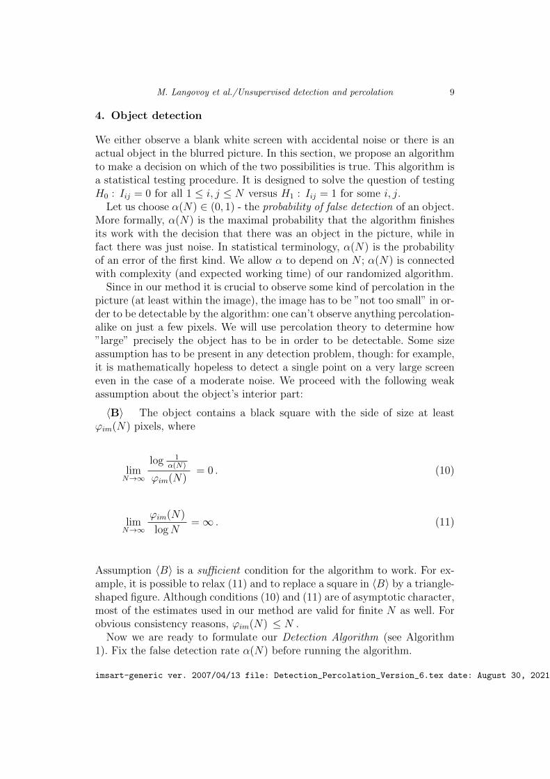
4. Object detection

We either observe a blank white screen with accidental noise or there is anactual object in the blurred picture. In this section, we propose an algorithmto make a decision on which of the two possibilities is true. This algorithm isa statistical testing procedure. It is designed to solve the question of testingH0 : Iij = 0 for all 1 ≤ i, j ≤ N versus H1 : Iij = 1 for some i, j.

Let us choose α(N) ∈ (0, 1) - the probability of false detection of an object.More formally, α(N) is the maximal probability that the algorithm finishesits work with the decision that there was an object in the picture, while infact there was just noise. In statistical terminology, α(N) is the probabilityof an error of the first kind. We allow α to depend on N ; α(N) is connectedwith complexity (and expected working time) of our randomized algorithm.

Since in our method it is crucial to observe some kind of percolation in thepicture (at least within the image), the image has to be ”not too small” in or-der to be detectable by the algorithm: one can’t observe anything percolation-alike on just a few pixels. We will use percolation theory to determine how”large” precisely the object has to be in order to be detectable. Some sizeassumption has to be present in any detection problem, though: for example,it is mathematically hopeless to detect a single point on a very large screeneven in the case of a moderate noise. We proceed with the following weakassumption about the object’s interior part:

〈B〉 The object contains a black square with the side of size at leastϕim(N) pixels, where

limN→∞

log 1α(N)

ϕim(N)= 0 . (10)

limN→∞

ϕim(N)

logN=∞ . (11)

Assumption 〈B〉 is a sufficient condition for the algorithm to work. For ex-ample, it is possible to relax (11) and to replace a square in 〈B〉 by a triangle-shaped figure. Although conditions (10) and (11) are of asymptotic character,most of the estimates used in our method are valid for finite N as well. Forobvious consistency reasons, ϕim(N) ≤ N .

Now we are ready to formulate our Detection Algorithm (see Algorithm1). Fix the false detection rate α(N) before running the algorithm.



Algorithm 1 Detection1: Step 0. Find an optimal θ(N) (in our framework θ(N) := 1/2).2: Step 1. Perform θ(N)−thresholding of the noisy picture Yi,jNi,j=1.3: Step 2.4: repeat5: Run depth-first search (Tarjan, 1972) on the graph GN of the θ(N)−thresholded

picture Y i,jNi,j=1

6: until Black cluster of size ϕim(N) is found or all black clusters are found7: Step 3.8: if black cluster of size ϕim(N) was found then9: Output: an object was detected

10: else11: Output: there is no object.12: end if

At Step 2 our algorithm finds and stores not only sizes of black clusters, butalso coordinates of pixels constituting each cluster. We remind that θ(N) isdefined as in (7), GN and Y i,jNi,j=1 were defined in Section 3, and ϕim(N)is any function satisfying (10). The depth-first search algorithm is a stan-dard procedure used for searching connected components on graphs. Thisprocedure is a deterministic algorithm. The detailed description and rigor-ous complexity analysis can be found in (Tarjan, 1972), or in the classic book(Aho et al., 1975), Chapter 5.

Let us prove that Algorithm 1 works, and determine its complexity.

Theorem 1. Suppose assumptions 〈A〉 and 〈B〉 are satisfied and the noiseis symmetric. Then

1. Algorithm 1 finishes its work in O(N2) steps, i.e. is linear.

2. If there was an object in the picture, Algorithm 1 detects it with prob-ability at least (1− exp(−C1(σ)ϕim(N))).

3. The probability of false detection doesn’t exceed minα(N), exp(−C2(σ)ϕim(N))for all N > N(σ).

The constants C1 > 0, C2 > 0 and N(σ) ∈ N depend only on σ.

Theorem 1 means that Algorithm 1 is of quickest possible order: it islinear in the input size in the worst case. Theorem 1 also implies that thealgorithm has computational complexity O(ϕim(N)) if the starting point ofthe depth-first search was close enough to the object. It is difficult to thinkof an algorithm working quicker in this problem. Indeed, if the image is verysmall and located in an unknown place on the screen, or if there is no imageat all, then any algorithm solving the detection problem will have to at least



upload information about O(N2) pixels, i.e. under general assumptions ofTheorem 1, any detection algorithm will have at least linear complexity.

Another important point is that Algorithm 1 is not only consistent, butthat it has exponential rate of accuracy, typically achievable only for para-metric or sufficiently smooth models.

Remark 1. It is also interesting to remark here that, although it is assumedthat the object of interest contains a ϕim(N) × ϕim(N) black square, onecannot use a very natural idea of simply considering sums of values on allsquares of size ϕim(N)× ϕim(N) in order to detect an object. Neither somesort of thresholding can be avoided, in general. Indeed, although this simpleidea works very well for normal noise, it cannot be used in case of unknownand possibly irregular or heavy-tailed noise. For example, for heavy-tailednoise, detection based on non-thresholded sums of values over subsquares willlead to a high probability of false detection. Whereas the method of the presentpaper still works.

5. Example

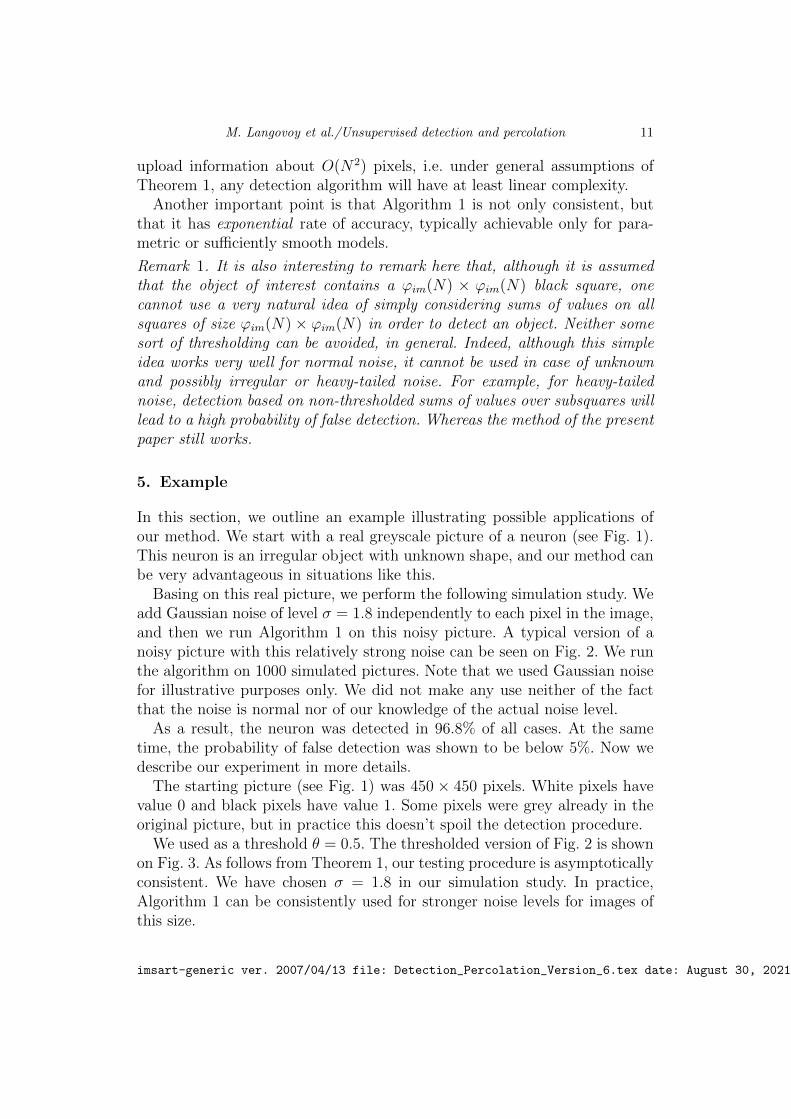
In this section, we outline an example illustrating possible applications ofour method. We start with a real greyscale picture of a neuron (see Fig. 1).This neuron is an irregular object with unknown shape, and our method canbe very advantageous in situations like this.

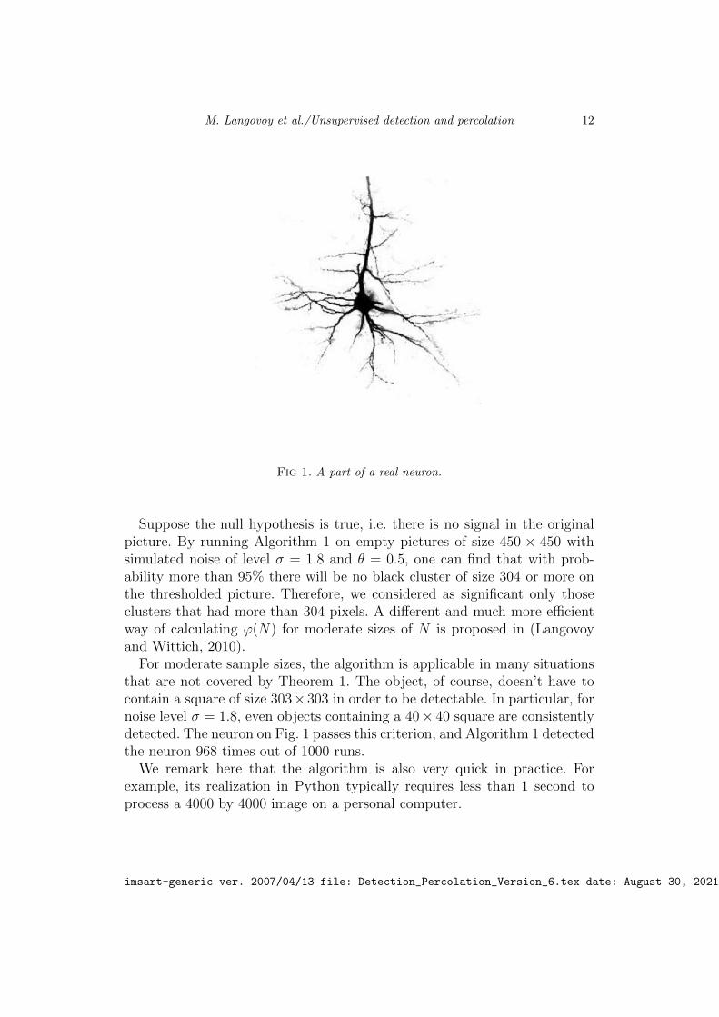
Basing on this real picture, we perform the following simulation study. Weadd Gaussian noise of level σ = 1.8 independently to each pixel in the image,and then we run Algorithm 1 on this noisy picture. A typical version of anoisy picture with this relatively strong noise can be seen on Fig. 2. We runthe algorithm on 1000 simulated pictures. Note that we used Gaussian noisefor illustrative purposes only. We did not make any use neither of the factthat the noise is normal nor of our knowledge of the actual noise level.

As a result, the neuron was detected in 96.8% of all cases. At the sametime, the probability of false detection was shown to be below 5%. Now wedescribe our experiment in more details.

The starting picture (see Fig. 1) was 450 × 450 pixels. White pixels havevalue 0 and black pixels have value 1. Some pixels were grey already in theoriginal picture, but in practice this doesn’t spoil the detection procedure.

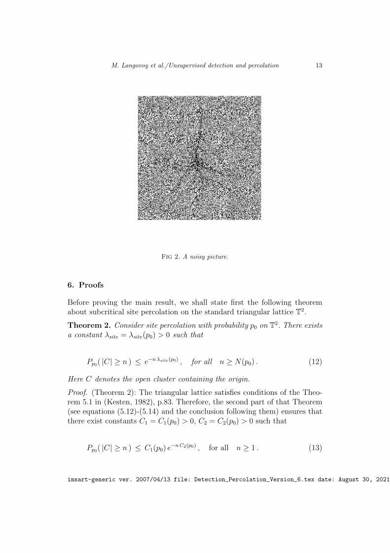
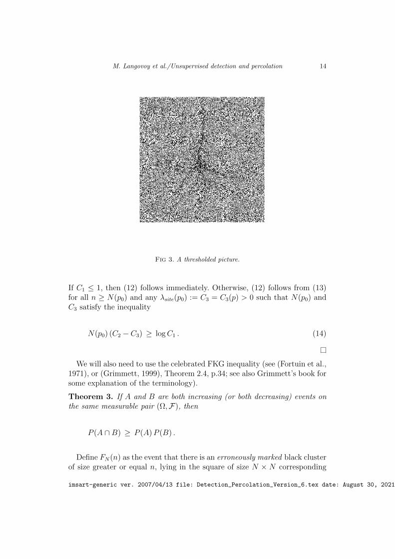
We used as a threshold θ = 0.5. The thresholded version of Fig. 2 is shownon Fig. 3. As follows from Theorem 1, our testing procedure is asymptoticallyconsistent. We have chosen σ = 1.8 in our simulation study. In practice,Algorithm 1 can be consistently used for stronger noise levels for images ofthis size.



Fig 1. A part of a real neuron.

Suppose the null hypothesis is true, i.e. there is no signal in the originalpicture. By running Algorithm 1 on empty pictures of size 450 × 450 withsimulated noise of level σ = 1.8 and θ = 0.5, one can find that with prob-ability more than 95% there will be no black cluster of size 304 or more onthe thresholded picture. Therefore, we considered as significant only thoseclusters that had more than 304 pixels. A different and much more efficientway of calculating ϕ(N) for moderate sizes of N is proposed in (Langovoyand Wittich, 2010).

For moderate sample sizes, the algorithm is applicable in many situationsthat are not covered by Theorem 1. The object, of course, doesn’t have tocontain a square of size 303×303 in order to be detectable. In particular, fornoise level σ = 1.8, even objects containing a 40× 40 square are consistentlydetected. The neuron on Fig. 1 passes this criterion, and Algorithm 1 detectedthe neuron 968 times out of 1000 runs.

We remark here that the algorithm is also very quick in practice. Forexample, its realization in Python typically requires less than 1 second toprocess a 4000 by 4000 image on a personal computer.



Fig 2. A noisy picture.

6. Proofs

Before proving the main result, we shall state first the following theoremabout subcritical site percolation on the standard triangular lattice T2.

Theorem 2. Consider site percolation with probability p0 on T2. There existsa constant λsite = λsite(p0) > 0 such that

Pp0( |C| ≥ n ) ≤ e−nλsite(p0) , for all n ≥ N(p0) . (12)

Here C denotes the open cluster containing the origin.

Proof. (Theorem 2): The triangular lattice satisfies conditions of the Theo-rem 5.1 in (Kesten, 1982), p.83. Therefore, the second part of that Theorem(see equations (5.12)-(5.14) and the conclusion following them) ensures thatthere exist constants C1 = C1(p0) > 0, C2 = C2(p0) > 0 such that

Pp0( |C| ≥ n ) ≤ C1(p0) e−nC2(p0) , for all n ≥ 1 . (13)



Fig 3. A thresholded picture.

If C1 ≤ 1, then (12) follows immediately. Otherwise, (12) follows from (13)for all n ≥ N(p0) and any λsite(p0) := C3 = C3(p) > 0 such that N(p0) andC3 satisfy the inequality

N(p0) (C2 − C3) ≥ logC1 . (14)

We will also need to use the celebrated FKG inequality (see (Fortuin et al.,1971), or (Grimmett, 1999), Theorem 2.4, p.34; see also Grimmett’s book forsome explanation of the terminology).

Theorem 3. If A and B are both increasing (or both decreasing) events onthe same measurable pair (Ω,F), then

P (A ∩B) ≥ P (A)P (B) .

Define FN(n) as the event that there is an erroneously marked black clusterof size greater or equal n, lying in the square of size N × N corresponding



to the screen. (An erroneously marked black cluster is a black cluster on GN

such that each of the pixels in the cluster was wrongly coloured black afterthe θ−thresholding).

Denote

pout(N) := P (Yij ≥ 1/2 | Imij = 0 ) , (15)

a probability of erroneously marking a white pixel outside of the image asblack.

The next theorem is particularly useful when studying percolation on finitesublattices of the initial infinite lattice.

Theorem 4. Suppose that 0 < pout(N) < psitec . There exists a constantC3 = C3(pout(N)) > 0 such that

Ppout(N)(FN(n)) ≤ exp(−nC3(pout(N))) , for all n ≥ ϕim(N) . (16)

Proof. (Theorem 4): Denote by C(i, j) the largest cluster in the N × Nscreen (triangulated by diagonals of one orientation) containing the pixelwith coordinates (i, j), and by C(0) the largest black cluster on the sameN × N screen containing 0. It doesn’t matter for this proof which point isdenoted by 0. By Theorem 2, for all i, j: 1 ≤ i, j ≤ N :

Ppout(N)( |C(0)| ≥ n ) ≤ e−nλsite(pout) , (17)

Ppout(N)( |C(i, j)| ≥ n ) ≤ e−nλsite(pout) .

Obviously, it only helped to inequalities (12) and (17) that we have limitedour clusters to only a finite subset instead of the whole lattice T2. On a sidenote, there is no symmetry anymore between arbitrary points of the N ×Nfinite subset of the triangular lattice; luckily, this doesn’t affect the presentproof.

Since |C(0)| ≥ n and |C(i, j)| ≥ n are increasing events (on themeasurable pair corresponding to the standard random-graph model on GN),we have that |C(0)| < n and |C(i, j)| < n are decreasing events for alli, j. By FKG inequality for decreasing events,

Ppout(N)( |C(i, j)| < n for all i, j, 1 ≤ i, j ≤ N ) ≥∏ ∏1≤i,j≤N

Ppout(N)( |C(i, j)| < n ) ≥ (by (17))

≥(

1− e−nλsite(pout))N2

.



It follows that

Ppout(N)(FN(n)) = Ppout(N)

(∃(i, j), 1 ≤ i, j ≤ N : |C(i, j)| ≥ n

)≤ 1−

(1− e−nλsite(pout)

)N2

= 1−N2∑k=0

(−1)k CkN2 e−nλsite(pout) k

=N2∑k=1

(−1)k−1CkN2 e−nλsite(pout) k

= N2e−nλsite(pout) + o(N2e−nλsite(pout)

),

because we assumed in (16) that n ≥ ϕim(N), and ϕim(N) logN . More-over, we see immediately that Theorem 4 follows now with some C3 suchthat 0 < C3(pout(N)) < λsite(pout(N)).

Now we establish the following useful lemma. Let GN denote the N × Nsubset of T2, as defined in Section 3 of the present paper. denote its canonicalmatching graph by G∗N . We remind that T2 is self-matching, and refer to(Kesten, 1982), Section 2.2 for the necessary definitions. Assuming that n ≤N , denote An be the event that there is an open (i.e., black) path in therectangle [0, n]× [0, n] joining some vertex on its left side to some vertex onits right side. Similarly, let Bn denote the event that there exists a closed(i.e., white) path on G∗n joining a vertex on the top side of G∗n to a vertex onits bottom side.

Remark 2. When speaking about black or white crossings of rectangles, weare free to assume that T2 is embedded in the plane as a Z2 lattice with diag-onals. See (Kesten, 1982) for a discussion of connections between percolationand various planar embeddings of regular lattices.

Lemma 1. Let 0 < p < 1 be a real number. Consider standard site percola-tion with probability p on the triangular lattice. Then

1. Either An or Bn occurs. Moreover, An ∩Bn = ∅ .2.

Pp(An) + Pp(Bn) = 1 . (18)

3.

Pp(An) + P1−p(An) = 1 . (19)



Proof. (Lemma 1). Statement 1 of the Lemma directly follows from Propo-sition 2.2 from (Kesten, 1982) (see also pp.398 - 402 of that book: there arigorous proof of this proposition is presented, including necessary topologi-cal considerations). Statement 2 is an immediate consequence of Statement1 and definitions of percolation measures on Gn and G∗n.

To complete the proof, note that GN and G∗N are isomorphic, by Example(iii), pp. 19-20 of (Kesten, 1982). Since by definition a vertex of G∗n is blackwith probability 1− p, we have that

Pp(Bn) = P1−p(An) . (20)

This proves (19).

First we prove the following theorem:

Theorem 5. Consider site percolation on T2 lattice with percolation prob-ability p > psitec = 1/2. Let An be the event that there is an open path inthe rectangle [0, n] × [0, n] joining some vertex on its left side to some ver-tex on its right side. Let Mn be the maximal number of vertex-disjoint openleft-right crossings of the rectangle [0, n] × [0, n]. Then there exist constantsC4 = C4(p) > 0, C5 = C5(p) > 0, C6 = C6(p) > 0 such that

Pp(An) ≥ 1− (n+ 1) e−C4 n , (21)

Pp(Mn ≤ C5 n ) ≤ e−C6 n , (22)

and both inequalities holds for all n ≥ N1(p).

Proof. (Theorem 5): Let LRk(n), 0 ≤ k ≤ n, be the event that the point(0, k) of Gn is connected by a white (in other words, closed) path (that liesin the interior of Gn) to some vertex on the right border of Gn. Denoteby LR(n) the event that there exists a closed left-right crossing of Gn. LetC((0, k)) denotes the white cluster containing the point (0, k), where wemake a convention that this cluster is considered on the whole lattice T2.Then obviously

LRk(n) ⊆ ω : |C((0, k))| ≥ n (23)



and

LR(n) ⊆n⋃k=0

LRk(n) . (24)

Now (24) gives us

P1−p(LR(n)) ≤n∑k=0

P1−p(LRk(n)) ≤ (n+ 1) max0≤k≤1

P1−p(LRk(n)) . (25)

Since 1− p < psitec , we get from (23) and Theorem 2 that for all k

P1−p(LRk(n)) ≤ P1−p( |C((0, k))| ≥ n ) ≤ e−C4 n . (26)

Combining (25) and (26) yields

P1−p(An) = P1−p(LR(n)) ≤ (n+ 1) e−C4 n . (27)

Altogether, (19) and (27) imply (21). This proves the first half of Theorem5.

As about the second part of the proof, (22) is deduced from (21) with thehelp of Theorem 2.45 of (Grimmett, 1999). The derivation itself is presentedat pp. 49-50 of (Grimmett, 1999); the only difference is that in our case onehas to change ”edges” by ”vertices” in the proof from the book. Everythingelse works the same, since Theorem 2.45 is valid for all Bernoulli productmeasures on regular lattices; in particular, Theorem 2.45 applies for sitepercolation as well. This completes the proof of Theorem 5.

Proof. (Theorem 1): I. First we prove the complexity result.The θ(N)−thresholding gives us Y i,jNi,j=1 and GN in O(N2) operations.

This finishes the analysis of Step 1.As for Step 2, it is known (see, for example, (Aho et al., 1975), Chapter 5,

or (Tarjan, 1972)) that the standard depth-first search finishes its work alsoin O(N2) steps. It takes not more than O(N2) operations to save positions ofall pixels in all clusters to memory , since one has no more than N2 positionsand clusters. This completes analysis of Step 2 and shows that Algorithm 1is linear in the size of the input data.



II. Now we prove the bound on the probability of false detection. Denote

pout(N) := P (Yij ≥ 1/2 | Imij = 0 ) , (28)

a probability of erroneously marking a white pixel outside of the image asblack. Under assumptions of Theorem 1, pout(N) < psitec . The exponentialbound on the probability of false detection follows trivially from Theorem 4.

III. It remains to prove the lower bound on the probability of true detec-tion. Suppose that we have an object in the picture that satisfies assumptionsof Theorem 1. Consider any ϕim(N) × ϕim(N) square in this image. Afterθ−thresholding of the picture by Algorithm 1, we observe on the selectedsquare a site percolation with probability

pim(N) := P (Yij ≥ 1/2 | Imij = 1 ) > psitec .

Then, by (21) of Theorem 5, there exists C4 = C4(pim(N)) such that therewill be at least one cluster of size not less than ϕim(N) (for example, onecould take any of the existing left-right crossings as a part of such cluster),provided that N is bigger than certain N1(pim(N)); and all that happenswith probability at least

1− n e−C4 n > 1− e−C3 n ,

for some C3: 0 < C3 < C4. Note that one can always weaken the constantC3 above in such a way that the estimate above starts to hold for all n ≥ 1.Theorem 1 is proved.

Acknowledgments. The authors would like to thank Remco van der Hofs-tad, Artem Sapozhnikov and Shota Gugushvili for helpful discussions.

References

Alfred V. Aho, John E. Hopcroft, and Jeffrey D. Ullman. The design andanalysis of computer algorithms. Addison-Wesley Publishing Co., Reading,Mass.-London-Amsterdam, 1975. Second printing, Addison-Wesley Seriesin Computer Science and Information Processing.



E. Arias-Castro and G. Grimmett. Cluster detection in networks using per-colation. Bernoulli, 19(2):676–719, 2013.

C. M. Fortuin, P. W. Kasteleyn, and J. Ginibre. Correlation inequalities onsome partially ordered sets. Comm. Math. Phys., 22:89–103, 1971. ISSN0010-3616.

Donald Geman and Bruno Jedynak. An active testing model for trackingroads in satellite images. IEEE Transactions on Pattern Analysis andMachine Intelligence, 18(1):1–14, 1996.

Geoffrey Grimmett. Percolation, volume 321 of Grundlehren der Mathematis-chen Wissenschaften [Fundamental Principles of Mathematical Sciences].Springer-Verlag, Berlin, second edition, 1999. ISBN 3-540-64902-6.

Harry Kesten. Percolation theory for mathematicians, volume 2 of Progressin Probability and Statistics. Birkhauser Boston, Mass., 1982. ISBN 3-7643-3107-0.

M. Langovoy and O. Wittich. Detection of objects in noisy images and sitepercolation on square lattices. EURANDOM Report No. 2009-035. EU-RANDOM, Eindhoven, 2009.

M. Langovoy and O. Wittich. Computationally efficient algorithms for sta-tistical image processing. Implementation in R. EURANDOM Report No.2010-053. EURANDOM, Eindhoven, 2010.

M. Langovoy and O. Wittich. Randomized algorithms for statistical imageanalysis and site percolation on square lattices. Statistica Neerlandica, 67(3):337–353, 2013a. ISSN 1467-9574. . URL http://dx.doi.org/10.

1111/stan.12010.M. Langovoy and O. Wittich. Robust nonparametric detection of objects in

noisy images. Journal of Nonparametric Statistics, 25(2):409–426, 2013b.M. Langovoy, M. Habeck, and B. Schoelkopf. Adaptive nonparametric de-

tection in cryo-electron microscopy. In Proceedings of the 58-th WorldStatistical Congress, Session: High Dimensional Data, pages 4456 – 4461,2011a.

M. Langovoy, M. Habeck, and B. Schoelkopf. Spatial statistics, image anal-ysis and percolation theory. In The Joint Statistical Meetings Proceedings,Time Series and Network Section, pages 5571 – 5581, American StatisticalAssociation, Alexandria, VA, 2011b.

Tim McInerney and Demetri Terzopoulos. Deformable models in medicalimage analysis: a survey. Medical image analysis, 1(2):91–108, 1996.

M. Negri, P. Gamba, G. Lisini, and F. Tupin. Junction-aware extractionand regularization of urban road networks in high-resolution sar images.Geoscience and Remote Sensing, IEEE Transactions on, 44(10):2962–2971,Oct. 2006. ISSN 0196-2892. .

Lucia Ricci-Vitiani, Dario G. Lombardi, Emanuela Pilozzi, Mauro Biffoni,


http://dx.doi.org/10.1111/stan.12010

http://dx.doi.org/10.1111/stan.12010


Matilde Todaro, Cesare Peschle, and Ruggero De Maria. Identificationand expansion of human colon-cancer-initiating cells. Nature, 445(7123):111–115, Oct. 2007. ISSN 0028-0836.

Yiye Ruan, David Fuhry, and Srinivasan Parthasarathy. Efficient communitydetection in large networks using content and links. In Proceedings ofthe 22nd international conference on World Wide Web, pages 1089–1098.ACM, 2013.

Sunil K. Sinha and Paul W. Fieguth. Automated detection of cracks in buriedconcrete pipe images. Automation in Construction, 15(1):58 – 72, 2006.ISSN 0926-5805. .

Robert Tarjan. Depth-first search and linear graph algorithms. SIAM J.Comput., 1(2):146–160, 1972. ISSN 0097-5397.

Jaewon Yang, Julian McAuley, and Jure Leskovec. Community detection innetworks with node attributes. In Data Mining (ICDM), 2013 IEEE 13thinternational conference on, pages 1151–1156. IEEE, 2013.


Unsupervised nonparametric detection of unknown objects …

Documents

Transcript of Unsupervised nonparametric detection of unknown objects …